 Zhiying Chen
 Zhaobin Du1*
- 1School of Electric Power Engineering, South China University of Technology, Guangzhou, China
- 2The Grid Planning and Research Center of Guangdong Power Grid Corporation, Guangzhou, China
With the trend of electronization of the power system, a traditional serial numerical algorithm is more and more difficult to adapt to the demand of real-time analysis of the power system. As one of the important calculating tasks in power systems, the online solution of Lyapunov equations has attracted much attention. A recursive neural network (RNN) is more promising to become the online solver of the Lyapunov equation due to its hardware implementation capability and parallel distribution characteristics. In order to improve the performance of the traditional RNN, in this study, we have designed an efficient vectorization method and proposed a reduced-order RNN model to replace the original one. First, a new vectorization method is proposed based on the special structure of vectorized matrix, which is more efficient than the traditional Kronecker product method. Second, aiming at the expanding effect of vectorization on the problem scale, a reduced-order RNN model based on symmetry to reduce the solution scale of RNN is proposed. With regard to the accuracy and robustness, it is proved theoretically that the proposed model can maintain the same solution as that of the original model and also proved that the proposed model is suitable for the Zhang neural network (ZNN) model and the gradient neural network (GNN) model under linear or non-linear activation functions. Finally, the effectiveness and superiority of the proposed method are verified by simulation examples, three of which are standard examples of power systems.
Introduction
With the trend of the electronic power system, the scale of system computing is increasing day by day, while the demand of real-time analysis and calculation in the process of system operation remains unchanged. Traditional serial algorithms cannot solve this contradiction well, so various parallel algorithms and distributed methods appear successively. In power system state estimation, Chen et al. (2017) have used the SuperLU_MT solver to estimate the state of the actual power grid, making full use of the parallel characteristics of multicore and multi-thread solver. Liu Z. et al. (2020) have fully explored the parallelism in the calculation of continuous power flow and applied the continuous Newton method power flow model to realize the parallel solution algorithm of continuous power flow based on GPU in large scale and multiple working conditions. Moreover, a novel distributed dynamic event-triggered Newton–Raphson algorithm is proposed to solve the double-mode energy management problem in a fully distributed fashion (Li et al., 2020). Similarly, Li Y. et al. (2019) proposed an event-triggered distributed algorithm with some desirable features, namely, distributed execution, asynchronous communication, and independent calculation, which can solve the issues of day-ahead and real-time cooperative energy management for multienergy systems. Given that software algorithms are essentially run by hardware, implementing functions directly from hardware is also an option for real-time computing. For example, Hafiz et al. (2020) proposed a real-time stochastic optimization of energy storage management using deep learning–based forecasts for residential PV applications, where the key of the real-time computation is the hardware controller. It is worth pointing out that compared with the aforementioned methods, the neural dynamics method has greater potential in the field of real-time calculation of power systems (Le et al., 2019), and its time constant can reach tens of milliseconds (Chicca et al., 2014) because of its parallel distribution characteristics and the convenience of hardware implementation.
The Lyapunov equation is widely used in some scientific and engineering fields to analyze the stability of dynamic systems (He et al., 2017; He and Zhang, 2017; Liu J. et al., 2020). In addition, the Lyapunov equation plays an important role in the controller design and robustness analysis of non-linear systems (Zhou et al., 2009; Raković and Lazar, 2014). In the field of power systems, the balanced truncation method, controller design, and stability analysis are also inseparable from the solution of the Lyapunov equation (Zhao et al., 2014; Zhu et al., 2016; Shanmugam and Joo, 2021). Therefore, many solving algorithms have been proposed to solve the Lyapunov equation. For example, Bartels and Stewart proposed the Bartels–Stewart method (Bartels and Stewart, 1972), which is a numerically stable solution. Lin and Simoncini (Lin and Simoncini, 2013) proposed the minimum residual method for solving the Lyapunov equation. Stykel (2008) used the low-rank iterative method to solve the Lyapunov equation and verified the effectiveness of the method through numerical examples. However, the efficiency of these serial processing algorithms is not high in large-scale applications and related real-time processing (Xiao and Liao, 2016).
Recently, due to its parallelism and convenience of hardware implementation, recurrent neural networks have been proposed and designed to solve the Lyapunov equation (Zhang et al., 2008; Yi et al., 2011; Yi et al., 2013; Xiao et al., 2019). The RNN mainly includes the Zhang neural network (ZNN) and gradient neural network (GNN) (Zhang et al., 2008). Most of the research studies on RNN focus on the improvement of model convergence. For example, Yi et al. (2013) point out that when solving a stationary or a non-stationary Lyapunov equation, the convergence of the ZNN is better than that of GNN. Yi et al. (2011) used a power-sigmoid activation function (PSAF) to build an improved GNN model to accelerate the iterative convergence of Lyapunov equation. In (Xiao and Liao, 2016), the sign-bi-power activation function (SBPAF) is used to accelerate the convergence of the ZNN model for solving the Lyapunov equation and the proposed ZNN model has finite-time convergence, which is obviously better than the previous ZNN and GNN models. In recent years, some studies have considered the noise-tolerant ZNN model. In Xiao et al. (2019), two robust non-linear ZNN (RNZNN) are established to find the solution of the Lyapunov equation under various noise conditions. Different from previous ZNN models activated by the typical activation functions (such as the linear activation function, the bipolar sigmoid activation function, and the power activation function), these two RNZNN models have predefined time convergence in the presence of various noises.
However, both GNN and ZNN need to transform the solution matrix from the matrix form to the vector form through the Kronecker product, which is called vectorization of the RNN model (Yi et al., 2011). The use of the Kronecker product will make the scale of the problem to be solved larger. As the size of the problem increases, the scaling effect of the Kronecker product becomes more obvious. The enlargement effect of the Kronecker product on the model size will not only lead to insufficient memory when the RNN is simulated on software but also make the hardware implementation of the RNN model need more devices and wiring, which increases the volume of hardware, the complexity of hardware production, and the failure rate of hardware. However, no study has discussed the order reduction of the RNN model.
It should be pointed out that the vectorized RNN model needs to be solved using a hardware circuit. However, as the relevant research of the RNN for solving the Lyapunov equation is still in the stage of theoretical exploration and improvement, there are no reports about hardware products of the RNN solver of the Lyapunov equation. Relevant studies (Zhang et al., 2008; Yi et al., 2011; Yi et al., 2013; Xiao and Liao, 2016; Xiao et al., 2019) simulate the execution process of the RNN hardware circuit through the form of software simulation, and this study also adopts this form. It is undeniable that the results of software simulation are consistent with those of hardware implementation. Therefore, the theoretical derivation and simulation results of the RNN in this article and in the literature (Zhang et al., 2008; Yi et al., 2011; Yi et al., 2013; Xiao and Liao, 2016; Xiao et al., 2019) can be extended to the scenarios of hardware implementation.
The RNN is used to solve the Lyapunov equation, and the ultimate goal is to develop an effective online calculation model to solve the Lyapunov equation, so it is of great significance to improve the calculation speed of the RNN. Current studies focus on improving the computational speed of the RNN by improving the convergence of RNN. However, how to efficiently realize vectorization of the RNN model is also a breakthrough to improve the computational efficiency of the RNN method. At present, the Kronecker product is generally used to transform the solution matrix into the vector form (Horn and Johnson, 1991). The Kronecker product actually performs multiple matrix multiplication operations, and the time complexity of multiplying two n×n matrices is O (n^3), so the time complexity of the Kronecker product increases rapidly as the scale increases. This means that the traditional matrix vectorization method based on the Kronecker product still has room for optimization.
In summary, this article proposes an efficient method for vectorizing the RNN model based on the special structure of the vectorized matrix, which is more efficient than the traditional expansion method by the Kronecker product. Aiming at the expanding effect of vectorization on the problem scale, a reduced-order RNN model based on symmetry was proposed for solving the time-invariant Lyapunov equation, and the validity and applicability of the reduced-order RNN model were proved theoretically. The main contributions of this article are as follows.
1) An efficient method for vectorization of RNN model is proposed. Compared with the traditional vectorization method, this method has higher efficiency and less time consumption.
2) The reduced-order RNN model for solving the Lyapunov equation based on symmetry is proposed, which greatly reduces the solution scale. It is proved theoretically that the proposed model can maintain the same solution as that of the original model. Meanwhile, it is proved theoretically that the proposed model is suitable for the ZNN model and GNN model under linear or non-linear activation functions.
3) Several simulation examples are given to verify the effectiveness and superiority of the proposed efficient method for vectorization of the RNN and the reduced-order RNN model. It is also verified that the neural dynamics method is suitable for solving the Lyapunov equation of power systems through three standard examples of power systems.
In order to show the contributions of this study more clearly, the logical graph using the RNN model for solving the Lyapunov equation is shown in Figure 1, and the main novelties and differences of this article from Refs Yi et al. (2011); Yi et al. (2013); Xiao and Liao (2016); Xiao et al. (2019) are shown in Table 1.
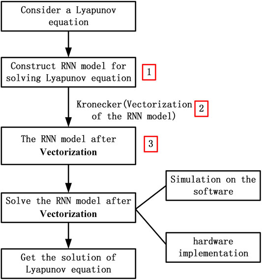
FIGURE 1. Logical graph of using a RNN model for solving the Lyapunov equation.
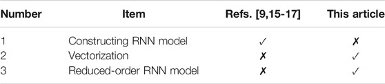
TABLE 1. Main novelties and differences of this article from the relevant references.
In Table1, items and numbers correspond to the three steps of Figure 1. The relevant references include Yi et al. (2011); Yi et al. (2013); Xiao and Liao (2016); Xiao et al. (2019).
In conclusion, Refs (Yi et al., 2011; Yi et al., 2013; Xiao and Liao, 2016; Xiao et al., 2019) focus on constructing a stronger RNN model to improve the convergence and noise-tolerant ability, including using different activation functions and neural networks. However, this study focuses on the vectorization method and the reduced-order RNN model.
Problem Formulation and Related Work
Problem Formulation
Consider the following well-known Lyapunov equation (Yunong Zhang and Danchi Jiang, 1995)
where A ∈ ℝn×n is a constant stable real matrix and C ∈ ℝn×n is a constant symmetric positive-definite matrix. The objective is to find the unknown matrix X(t) ∈ ℝn×n to make the Lyapunov matrix Eq. 1 hold true. Let
GNN
According to the principle of GNN (Yi et al., 2011) and combined with the characteristics of Lyapunov equation, a corresponding GNN model can be designed to solve the Lyapunov equation. The design steps are as follows:
First, construct an energy function based on norm as follows:
where
Second, based on the principle of the negative gradient descent of the GNN, the following formula can be constructed:
By introducing the adjustable positive parameter
where
Finally, the conventional linear GNN (Eq. 4) can be improved into the following non-linear expression by employing a non-linear activation function array
where
where
ZNN
First, following Zhang et al.’s design method (Zhang et al., 2002), we can define the following matrix-valued error function to monitor the solution process of Lyapunov Eq. 1:
Then in view of the definition of
where
In this study, the RNZNN-1 model is selected as the representative of the non-linear activation function of the ZNN model for simulation because of its strong convergence (Xiao et al., 2019). The expression of the non-linear activation function in the RNZNN-1 model is as follows:
where design parameters
An Efficient Method for Vectorization of RNN Model
General Method of Vectorizing RNN Model
The RNN model needs to be transformed to the vector form so that it can be used for software simulation (Li X. et al., 2019) and hardware implementation.
Vectorization of the GNN Model
Yi et al. (2011) pointed out that the vectorization of GNN model is as follows:
where
where
Since the order of matrix addition and matrix transpose is interchangeable (Cheng and Chen, 2017),
Applying this property to Eq. 11, we can get
According to Chen and Zhou (2012), the relationship between the matrix transpose and Kronecker product is as follows:
Applying this property to Eq. 14, we can get
Considering
Vectorization of the ZNN Model
The vectorization process of the ZNN model is similar to that of the GNN. Carry out Kronecker product on Eq. 8, and we can get:
Vectorization of the RNN Model
By comparing Eqs 10, 17 and 18, it can be seen that the key of vectorization of the RNN model is to solve
According to Eq. 12, the calculation of
1) Calculate
where
2) Calculate
where
3) Add
An Efficient Method for Vectorization of RNN Model
According to the previous analysis, no matter how the matrix
1) Create a matrix with
2) Fill
3) Add the corresponding element of
The vectorization method of the RNN model proposed in this article is still based on the Kronecker product, but the time complexity is greatly reduced. Because the vectorization method proposed in this article replaces matrix multiplication with assignment and addition.
The Reduced-Order RNN Model for Solving Lyapunov Equations Based on Symmetry
Since the solution of Eq. 1,
The Reduced-Order ZNN Model With Linear Activation Function
Vectorization
Let’s consider a ZNN model with linear activation function after vectorization. The formula is as follows:
where
For the convenience of later discussion, S∈
Each element of
We can expand
Reduce the Column Number of
If the Kronecker product is directly carried out on Eq. 1, then
We can use
Multiply both sides of Eq. 22 by the inverse matrix of
From Eq. 25, we can see that
Reduce the Row Number of
When the steady state is considered, the differential term of Eq. 26 is 0, and we can get:
As mentioned before, if
We can construct the augmented matrix of Eq. 27 and name it as
According to the knowledge of linear algebra, the vector set
Let us define the vectors which can be represented linearly by the other vectors as the redundant vectors. Suppose that
where
According to the aformentioned analysis, as long as
For a redundant vector, its own row index and the row index of another vector equal to it can form a pair of indexes. We can use these index pairs to find the redundant vectors and delete the corresponding rows. In general, in an index pair, the equation corresponding to the index whose value is larger is selected for deletion.
After the row deletion, the row number of
We can use
Reduced-Order GNN Model With Linear Activation Function
Consider a GNN model with linear activation function after vectorization. The formula is as follows:
When the steady state is considered, the differential term of Eq. 30 is 0, and Eq. 30 is changed into Eq. 24. From the aforementioned derivation, it can be known that both
When the steady state is considered, Eq. 31 is changed into
Reduced-Order RNN Model With Non-Linear Activation Functions
Before every non-linear activation function is introduced into the linear RNN, it will be theoretically proved that their introduction can guarantee the correct convergence of RNN. However, the reduced-order RNN in this article does not change the structure of RNN, but only changes the size of RNN. Because both the problem scale and the specific values of the matrix are generally expressed in symbolic form in the theoretical derivation (Xiao and Liao, 2016; Xiao et al., 2019), and the reduced-order RNN model in this article is still applicable to the relevant theoretical proof of introducing the non-linear activation functions into the linear RNN. In other words, the reduced-order method in this article can be applied to the RNN model with non-linear activation functions.
The Generation of the Reduced-Order RNN Model
The steps for generating the reduced-order RNN model are as follows:
1)
2) Considering that the indexes in the symmetric positions of
3) For
4) For
It should be pointed out that in mathematical proof, if the order of row reduction and column reduction is exchanged, the correctness of the reduced-order RNN model cannot be proved or another proof method is needed to complete the proof. However, in the case that the mathematical proof has been completed, the order of row reduction and column reduction does not affect the final result, since we know in advance which rows and columns are to be deleted. In the aformentioned steps of generating the reduced-order RNN model, the reason why we carry out step 3 first is that it can reduce the computational amount of the column addition to achieving higher computational efficiency.
The Significance of the Reduced-Order RNN Model
In order to better explain the value and significance of the reduced-order RNN model proposed in this article, the differences before and after the order reduction are shown from the perspectives of software simulation and hardware implementation, respectively. For the convenience of discussion, the GNN is taken as an example to illustrate.
Simulation on the Software
We use the ode45 function of MATLAB to solve the GNN model after vectorization. By comparing Eq. 30 and Eq. 31, it can be seen that the memory requirement of the reduced-order GNN model is much smaller than that of the original GNN model. Therefore, the reduced-order GNN model greatly alleviates the problem of insufficient memory that may occur in the software simulation of the GNN.
Hardware Implementation
When we use the traditional GNN model, the structure of the circuit diagram is shown as Figure 2 (Yi et al., 2011).

FIGURE 2. Circuit schematics which realizes GNN.
Where
When we use the reduced-order GNN model, the structure of the circuit diagram is shown as Figure 2, except that the
So the reduced-order GNN model greatly reduces the number of devices and wiring required for the hardware realization of GNN model, which is conducive to reducing the volume of hardware, the complexity of hardware production, and the failure rate of hardware.
Illustrative Verification
The simulation examples in this article are all completed on the MATLAB 2013b platform. In this article, the ode45 function of MATLAB is used to simulate the iterative process of RNN (Zhang et al., 2008). The corresponding computing performance is tested on a personal computer with Intel Core i7-4790 CPU @3.2GHz and 8 GB RAM.
Since there are great differences between software and hardware in the principle of realizing the integral function, there will be a big gap between the time cost in simulating the RNN process using software and the time cost in implementing the RNN model using hardware. Considering the research on the RNN model used to solve the Lyapunov equation is still in the stage of theoretical exploration, and has not reached the stage of hardware production for the time being, this article does not discuss the influence of the proposed reduced-order RNN model on the time consuming of RNN.
The Reduced-Order RNN Model for Solving Lyapunov Equation Based on Symmetry
Example 1
Let us consider the Lyapunov Eq. 1 with the following coefficient matrices:
where
In this example, we set
In order to demonstrate the advantages of the reduced-order RNN model, this article compares the performance of the reduced-order RNN and the original-order RNN, as shown in Table 2. In Table 2, linearity and non-linearity, respectively, mean the linear activation function and the non-linear activation function. Scale means the row number of

TABLE 2. Comparison of the original-order RNN and the reduced-order RNN under Example 1.
In order to study the effect of order reduction method proposed in this article on the convergence of the RNN model, the F-norm curves of the original-order RNN model and the reduced-order RNN model are drawn, as shown in Figure 3. In Figure 3A, LAF means the ZNN model with linear activation functions. NAF means the ZNN model with the non-linear activation function of Eq. 9. In Figure 3B, LAF means the GNN model with linear activation functions. BPAF means the GNN model with the non-linear activation function of Eq. 6. In both Figure 3A and Figure 3B, F-norm refers to
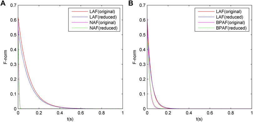
FIGURE 3. Comparison of the convergence between the original-order and the reduced-order RNN models under Example 1. (A) is ZNN, (B) is GNN.
Example 2
To enlarge the scale of the example, we consider Lyapunov Eq. 1 with the following coefficient matrices:
where
In this example, RNN’s model parameters are the same as Example 1. Similar to Example 1, we can get Table 3 and Figure 4. The definitions of all nouns in Table 3 are the same as those in Table 2, and the definitions of all nouns in Figure 4 are the same as those in Figure 3.

TABLE 3. Comparison of the original-order RNN and the reduced-order RNN under Example 2.
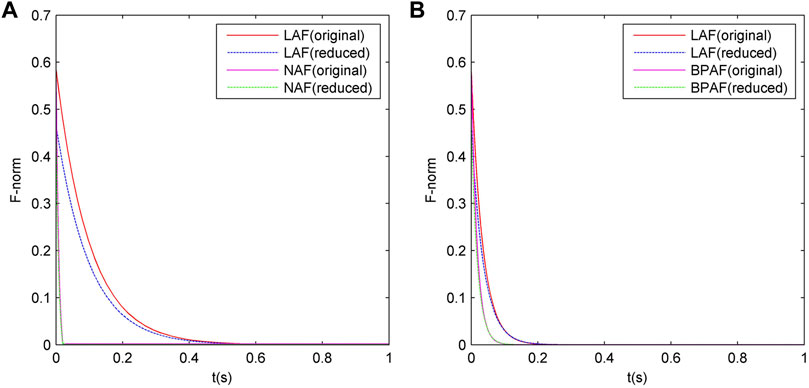
FIGURE 4. Comparison of the convergence between the original-order and the reduced-order RNN models under Example 2. (A) is ZNN, (B) is GNN.
Example 3
A 10∗10 matrix is randomly generated and then α-shift is applied to the matrix to make it stable (Yang et al., 1993), which is the generation process of
In this example, RNN’s model parameters are the same as Example 1. Similar to Example 1, we can get Table 4 and Figure 5. The definitions of all nouns in Table 4 are the same as those in Table 2, and the definitions of all nouns in Figure 5 are the same as those in Figure 3.

TABLE 4. Comparison of the original-order RNN and the reduced-order RNN under Example 3.
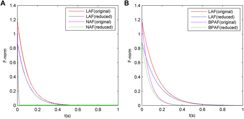
FIGURE 5. Comparison of the convergence between the original-order and the reduced-order RNN models under Example 3. (A) is ZNN, (B) is GNN.
Based on the information in the aforementioned three tables, we can draw the following conclusions:
a) The reduced-order RNN model has a very obvious effect, with the scale reduced by about 33–45%. Moreover, the effect of the reduced-order RNN model becomes more obvious with the increase in the size of the example. According to
b) Under different case scales, whether it is ZNN or GNN, whether it is linear activation function or non-linear activation function, the steady-state errors of the reduced-order RNN model are very close to 0, which means the reduced-order RNN model can always converge to the correct solution of the Lyapunov equation. This indicates that the reduced-order RNN model is applicable to ZNN and GNN, as well as the scenarios of linear activation function and non-linear activation function, which is consistent with the theoretical derivation results above.
c) Under different case scales, the difference in the steady-state accuracy between the reduced-order RNN and the original-order RNN is very small, indicating that the reduced-order RNN basically does not affect the steady-state accuracy of RNN.
Based on the information in the aforementioned three figures, we can draw the following conclusions:
a) Under different case scales, the reduced-order RNN models with linear or non-linear activation functions either have a little effect on the iterative convergence characteristics or enhance the convergence at the beginning of the iteration process and have a little effect on the convergence at the end of it.
b) Under the non-linear activation functions, the convergence of the ZNN model is always stronger than that of the GNN model when other conditions are fixed.
c) Under the linear activation function, the convergence of the ZNN model is weaker than that of the GNN model when the size of the examples is small (e.g., Example 1 and Example 2). The convergence of the linear ZNN model is stronger than that of the linear GNN model when the size of the examples is large (e.g., Example 3).
d) For both ZNN and GNN, the convergence of the RNN model with non-linear activation function is always stronger than that of the linear RNN model.
e) With the increase in the size of the examples, the convergence of ZNN is basically unchanged, while the convergence of GNN will become significantly worse.
Example 4
In order to verify the applicability of neural dynamics method to the power system, the corresponding Lyapunov equation describing system controllability is generated for the IEEE three-machine nine-node system according to the principle of the balanced truncation method in (Zhao et al., 2014). The input signal is the rotor speed deviation and the output signal is the auxiliary stabilizing signal (Zhu et al., 2016). It should be noted that the IEEE standard systems used in this article come from the examples of the PST toolkit (Lan, 2017), and the linearization process of the system is realized by the svm_mgen.m of PST toolkit. We set
In this example, the linear ZNN was selected for testing. Similar to Example 1, we can get Table 5 and Figure 6. The definitions of all nouns in Table 5 are the same as those in Table 2 and the definitions of all nouns in Figure 6 are the same as those in Figure 3.

TABLE 5. Comparison of the original-order ZNN and the reduced-order ZNN under Examples 4-6.
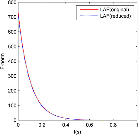
FIGURE 6. Comparison of the convergence between the original-order and the reduced-order ZNN models under Example 4.
Example 5
Similar to Example 4, we generate the corresponding Lyapunov equation describing system controllability of the IEEE 16-machine system. A ∈
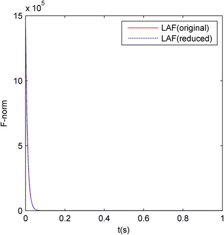
FIGURE 7. Comparison of the convergence between the original-order and the reduced-order ZNN models under Example 5.
Example 6
Similar to Example 4, we generate the corresponding Lyapunov equation describing system controllability of the IEEE 48-machine system. A ∈
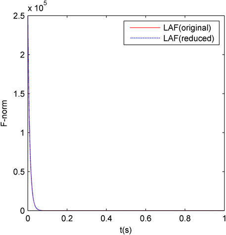
FIGURE 8. Comparison of the convergence between the original-order and the reduced-order ZNN models under Example 6.
It can be seen from Table 5 and Figures 6–8 that the neural dynamics method used to solve Lyapunov equations is also suitable for solving Lyapunov equations in power systems, and the reduced-order RNN mosdels proposed in this article is effective in the example of power systems. Moreover, with the increase in the power system scale, the convergence and steady-state accuracy of ZNN model are almost unchanged, indicating the applicability of the RNN model to power systems of different scales.
It is worth mentioning that the integration between the electric power and natural gas systems has been steadily enhanced in recent decades. The incorporation of natural gas systems brings, in addition to a cleaner energy source, greater reliability and flexibility to the power system (Liu et al., 2021). Since the dynamic model of the electricity–gas coupled system can be expressed by differential-algebraic equations (Zhang, 2005; Yang, 2020), which means the dynamic model of the electricity–gas coupled system is the same as that of the power system, the aforementioned applicability analysis of the methods proposed in this article for large power systems are also applicable to large electricity–gas coupled systems.
An Efficient Method for Vectorization of RNN Model
Table 6 compares the time cost of the RNN model vectorization method proposed in this article and the traditional RNN model vectorization method. For the sake of convenience, the former is called method A and the latter is called method B. In order to better demonstrate the effect of the vectorization method of RNN model proposed in this article, four examples are added, as shown in Table 6. Four newly added examples are generated in the same way as Example 3 and are detailed in Supplementary Material, where ms means millisecond; scale means the order of
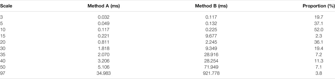
TABLE 6. Comparison of the time cost of two vectorization methods for RNN models.
It can be seen from Table 6 that method A is significantly better than method B in terms of time cost, with the decrease in time cost between 48 and 98%. With the increase in the size of the examples, the proportion of time cost improvement generally increases. It should be pointed out that when the system sizes are 15, 35, and 97, the corresponding examples are the IEEE standard systems mentioned before, which indicates that the vectorization method proposed in this article is also effective in the example of power systems.
Conclusion
1) We propose an efficient method for vectorizing RNN models, which can achieve higher computational efficiency than the traditional method of vectorizing RNN based on the Kronecker product.
2) In order to reduce the solving scale of the RNN model, a reduced-order RNN model for solving the Lyapunov equation was proposed based on symmetry. At the same time, it is proved theoretically that the proposed model can maintain the same solution as that of the original model, and it is also proved that the proposed model is suitable for both the ZNN model and GNN model under linear or non-linear activation functions.
3) Several simulation examples are given to verify the effectiveness and superiority of the proposed method, while three standard examples of power systems are given to verify that the neural dynamics method is suitable for solving the Lyapunov equation of power systems.
Because the neural dynamics method has parallel distribution characteristics and hardware implementation convenience, its convergence and computation time are not sensitive to the system scale. Considering the current development level and trend of the very large-scale integration (VLSI) chip and the ultra large-scale integration (ULSI) chip, the wide application of the neural dynamics method in large-scale systems is expected.
In addition, the research on the RNN model used to solve the Lyapunov equation is mainly in the stage of theoretical improvement and exploration, and there are few reports about hardware products. The hardware product design will be the main content of the next stage.
Data Availability Statement
The original contributions presented in the study are included in the article/Supplementary Material, further inquiries can be directed to the corresponding author.
Author Contributions
All authors listed have made a substantial, direct, and intellectual contribution to the work and approved it for publication.
Funding
This work was supported in part by the Key-Area Research and Development Program of Guangdong Province (2019B111109001), the National Natural Science Foundation of China (51577071), and the Southern Power Grid Corporation’s Science and Technology Project (Project No. 037700KK52190015 (GDKJXM20198313)).
Conflict of Interest
The authors declare that the research was conducted in the absence of any commercial or financial relationships that could be construed as a potential conflict of interest.
Publisher’s Note
All claims expressed in this article are solely those of the authors and do not necessarily represent those of their affiliated organizations, or those of the publisher, the editors, and the reviewers. Any product that may be evaluated in this article, or claim that may be made by its manufacturer, is not guaranteed or endorsed by the publisher.
Supplementary Material
The Supplementary Material for this article can be found online at: https://www.frontiersin.org/articles/10.3389/fenrg.2022.796325/full#supplementary-material
References
Bartels, R. H., and Stewart, G. W. (1972). Solution of the Matrix Equation AX + XB = C [F4]. Commun. ACM 15 (9), 820–826. doi:10.1145/361573.361582
Chen, Q., Gong, C., Zhao, J., Wang, Y., and Zou, D. (2017). Application of Parallel Sparse System Direct Solver Library Super LU_MT in State Estimation. Automation Electric Power Syst. 41 (3), 83–88. doi:10.7500/AEPS20160607008
Chicca, E., Stefanini, F., Bartolozzi, C., and Indiveri, G. (2014). Neuromorphic Electronic Circuits for Building Autonomous Cognitive Systems. Proc. IEEE 102 (9), 1367–1388. doi:10.1109/JPROC.2014.2313954
Hafiz, F., Awal, M. A., Queiroz, A. R. d., and Husain, I. (2020). Real-Time Stochastic Optimization of Energy Storage Management Using Deep Learning-Based Forecasts for Residential PV Applications. IEEE Trans. Ind. Applicat. 56 (3), 2216–2226. doi:10.1109/TIA.2020.2968534
He, W., and Zhang, S. (2017). Control Design for Nonlinear Flexible Wings of a Robotic Aircraft. IEEE Trans. Contr. Syst. Technol. 25 (1), 351–357. doi:10.1109/TCST.2016.2536708
He, W., Ouyang, Y., and Hong, J. (2017). Vibration Control of a Flexible Robotic Manipulator in the Presence of Input Deadzone. IEEE Trans. Ind. Inf. 13 (1), 48–59. doi:10.1109/TII.2016.2608739
Horn, R. A., and Johnson, C. R. (1991). Topics in Matrix Analysis. Cambridge: Cambridge University Press.
Lan, X. (2017). Research on Model Order Reduction Method and Predictive Control Algorithm of Grid Voltage Control System (Beijing: North China Electric Power University). [dissertation/master’s thesis].
Le, X., Chen, S., Li, F., Yan, Z., and Xi, J. (2019). Distributed Neurodynamic Optimization for Energy Internet Management. IEEE Trans. Syst. Man. Cybern, Syst. 49 (8), 1624–1633. doi:10.1109/TSMC.2019.2898551
Li, X., Yu, J., Li, S., Shao, Z., and Ni, L. (2019a). A Non-linear and Noise-Tolerant ZNN Model and its Application to Static and Time-Varying Matrix Square Root Finding. Neural Process. Lett. 50 (2), 1687–1703. doi:10.1007/s11063-018-9953-y
Li, Y., Zhang, H., Liang, X., and Huang, B. (2019b). Event-Triggered-Based Distributed Cooperative Energy Management for Multienergy Systems. IEEE Trans. Ind. Inf. 15 (4), 2008–2022. doi:10.1109/TII.2018.2862436
Li, Y., Gao, D. W., Gao, W., Zhang, H., and Zhou, J. (2020). Double-Mode Energy Management for Multi-Energy System via Distributed Dynamic Event-Triggered Newton-Raphson Algorithm. IEEE Trans. Smart Grid 11 (6), 5339–5356. doi:10.1109/TSG.2020.3005179
Lin, Y., and Simoncini, V. (2013). Minimal Residual Methods for Large Scale Lyapunov Equations. Appl. Numer. Maths. 72, 52–71. doi:10.1016/j.apnum.2013.04.004
Liu, J., Zhang, J., and Li, Q. (2020a). Upper and Lower Eigenvalue Summation Bounds of the Lyapunov Matrix Differential Equation and the Application in a Class Time-Varying Nonlinear System. Int. J. Control. 93 (5), 1115–1126. doi:10.1080/00207179.2018.1494389
Liu, Z., Chen, Y., Song, Y., Wang, M., and Gao, S. (2020b). Batched Computation of Continuation Power Flow for Large Scale Grids Based on GPU Parallel Processing. Power Syst. Techn. 44 (3), 1041–1046. doi:10.13335/j.1000-3673.pst.2019.2050
Liu, H., Shen, X., Guo, Q., and Sun, H. (2021). A Data-Driven Approach towards Fast Economic Dispatch in Electricity-Gas Coupled Systems Based on Artificial Neural Network. Appl. Energ. 286, 116480. doi:10.1016/j.apenergy.2021.116480
Raković, S. V., and Lazar, M. (2014). The Minkowski-Lyapunov Equation for Linear Dynamics: Theoretical Foundations. Automatica 50 (8), 2015–2024. doi:10.1016/j.automatica.2014.05.023
Shanmugam, L., and Joo, Y. H. (2021). Stability and Stabilization for T-S Fuzzy Large-Scale Interconnected Power System with Wind Farm via Sampled-Data Control. IEEE Trans. Syst. Man. Cybern, Syst. 51 (4), 2134–2144. doi:10.1109/TSMC.2020.2965577
Stykel, T. (2008). Low-rank Iterative Methods for Projected Generalized Lyapunov Equations. Electron. Trans. Numer. Anal. 30 (1), 187–202. doi:10.1080/14689360802423530
Xiao, L., and Liao, B. (2016). A Convergence-Accelerated Zhang Neural Network and its Solution Application to Lyapunov Equation. Neurocomputing 193, 213–218. doi:10.1016/j.neucom.2016.02.021
Xiao, L., Zhang, Y., Hu, Z., and Dai, J. (2019). Performance Benefits of Robust Nonlinear Zeroing Neural Network for Finding Accurate Solution of Lyapunov Equation in Presence of Various Noises. IEEE Trans. Ind. Inf. 15 (9), 5161–5171. doi:10.1109/TII.2019.2900659
Yang, J., Chen, C. S., Abreu-garcia, J. A. D., and Xu, Y. (1993). Model Reduction of Unstable Systems. Int. J. Syst. Sci. 24 (12), 2407–2414. doi:10.1080/00207729308949638
Yang, H. (2020). Dynamic Modeling and Stability Studies of Integrated Energy System of Electric, Gas and Thermal on Multiple Time Scales (Hunan: Changsha University of Science & Technology). [dissertation/master’s thesis].
Yi, C., Chen, Y., and Lu, Z. (2011). Improved Gradient-Based Neural Networks for Online Solution of Lyapunov Matrix Equation. Inf. Process. Lett. 111 (16), 780–786. doi:10.1016/j.ipl.2011.05.010
Yi, C., Chen, Y., and Lan, X. (2013). Comparison on Neural Solvers for the Lyapunov Matrix Equation with Stationary & Nonstationary Coefficients. Appl. Math. Model. 37 (4), 2495–2502. doi:10.1016/j.apm.2012.06.022
Yunong Zhang, Z., and Danchi Jiang, M. T. J. (1995). A Recurrent Neural Network for Solving Sylvester Equation with Time-Varying Coefficients. New York: Academic Press.
Zhang, Y., Jiang, D., and Wang, J. (2002). A Recurrent Neural Network for Solving Sylvester Equation with Time-Varying Coeffificients. IEEE Trans. Neural Netw. 13 (5), 1053–1063. doi:10.1109/TNN.2002.1031938
Zhang, Y., Chen, K., Li, X., Yi, C., and Zhu, H. (2008). “Simulink Modeling and Comparison of Zhang Neural Networks and Gradient Neural Networks for Time-Varying Lyapunov Equation Solving,” in Proceedings of IEEE International Conference on Natural Computation. Jinan. IEEE, 521–525. doi:10.1109/ICNC.2008.47
Zhang, Y. (2005). Study on the Methods for Analyzing Combined Gas and Electricity Networks (Beijing: China Electric Power Research Institute). [dissertation/master’s thesis].
Zhao, H., Lan, X., Xue, N., and Wang, B. (2014). Excitation Prediction Control of Multi‐machine Power Systems Using Balanced Reduced Model. IET Generation, Transm. Distribution 8 (6), 1075–1081. doi:10.1049/iet-gtd.2013.0609
Zhou, B., Duan, G.-R., and Li, Z.-Y. (2009). Gradient Based Iterative Algorithm for Solving Coupled Matrix Equations. Syst. Control. Lett. 58 (5), 327–333. doi:10.1016/j.sysconle.2008.12.004
Keywords: Lyapunov equation, vectorization, reduced-order RNN, symmetry, ZNN, GNN
Citation: Chen Z, Du Z, Li F and Xia C (2022) A Reduced-Order RNN Model for Solving Lyapunov Equation Based on Efficient Vectorization Method. Front. Energy Res. 10:796325. doi: 10.3389/fenrg.2022.796325
Received: 16 October 2021; Accepted: 03 January 2022;
Published: 07 February 2022.
Edited by:
Yan Xu, Nanyang Technological University, SingaporeCopyright © 2022 Chen, Du, Li and Xia. This is an open-access article distributed under the terms of the Creative Commons Attribution License (CC BY). The use, distribution or reproduction in other forums is permitted, provided the original author(s) and the copyright owner(s) are credited and that the original publication in this journal is cited, in accordance with accepted academic practice. No use, distribution or reproduction is permitted which does not comply with these terms.
*Correspondence: Zhaobin Du, ZXBkdXpiQHNjdXQuZWR1LmNu