Abstract
Series arc fault is the main cause of electrical fire in low-voltage distribution system. A fast and accurate detection system can reduce the risk of fire effectively. In this paper, series arc experiment is carried out for different kinds of electrical load. The time-domain current is analyzed by Morlet wavelet. Then, the multiscale wavelet coefficients are expressed as the coefficient matrix. In order to meet the data dimension requirements of neural networks, a color domain transformation method is used to transform the feature matrix into an image. A regularization method based on gamma transform is proposed for small sample data sets. The results showed that the proposed regularization method improved the validation set accuracy of ResNet50 from 66.67% to 96.53%. The overfitting problem of neural network was solved. In addition, this method fused fault features of 64 different scales, and provided a valuable manually labeled arc fault dataset. Compared with the threshold detection method, this method was more objective. The use of image features increased intuitiveness and generality. Compared with other typical lightweight networks, this method had the best detection performance.
1 Introduction
1.1 Introduction to arc faults
Arc is a kind of abnormal discharge phenomenon in insulating medium. The arc can keep burning when the circuit voltage is higher than 20 V and the current is greater than 0.1A (Qu and Wang, 2018). It is easy to injure people or produce electrical fire. In low-voltage power distribution system, arc fault may be caused by irregular circuit connection and the aging electronic equipment. When series arc fault occurs, the residual current of the circuit is usually less than the cut-off threshold of low-voltage circuit breaker. The circuit cannot be cut off in time. A real-time and accurate arc fault detection system can reduce the risk of fire effectively.
In the 1940s, Cassie and Mayr established the arc model by studying the relationship between arc dissipated power and current. Since then, the research on arc faults mainly focuses on the simulation of arc models. As these two arc models are suitable for circuits with different voltages, some studies are aimed at improving and integrating the arc model to make it applicable to more occasions (Xiang and Wang, 2019) (Shu and Wang, 2018).
1.2 Research gap
In recent years, the researches of arc fault detection are not limited to the arc mathematical model. In fact, some circuit parameters may have a mutation when an arc fault occurs. The purpose of fault detection can be achieved by identifying the circuit parameters as features. In practical application, it is difficult to collect the photothermal physical characteristics of the arc in real time due to the random arc generation. As a result, the common feature extraction method is time-frequency domain analysis of voltage or current. Fast Fourier analysis (FFT) is the main method of frequency domain analysis. In addition, literature (Humbert et al., 2021) realizes the detection of series arc faults of different loads through the change rate of voltage spectral dispersion index (SDI) of low-voltage power line. Literature (Chu et al., 2020) designed a high-frequency coupling sensor to detect the high-frequency characteristics of arc generation, and established a fault identification model according to the different high-frequency characteristics of different loads. In literature (Joga et al., 2021), time-domain information and frequent-domain information are fused by wavelet analysis. The fused features are fed into the convolutional neural network for detection.
The extraction of time domain features has also changed from the original phase analysis to empirical mode analysis (EMD) or noise processing (Ji et al., 2020; Lala and Subrata, 2020; Cui and Tong, 2021). However, a single feature has great uncertainty in the face of arc faults with many singularities. The fusion of fault feature has become a new challenge in the research of detection method.
As a time-frequency analysis method, the multi-resolution characteristic of wavelet analysis is efficient in many fields. The fusion of fault features in time-frequency domain ensures the real-time detection (Xiong and Chen, 2020) (Liu and Du, 2017).
In addition, some statistics of the circuit can also be used as fusion features, such as information entropy wavelet energy entropy and power spectrum entropy of signal (Cui and Li, 2021a) or the fusion of proportional coefficient of arc zero rest time and normalization coefficient of low-pass filter (Zhao and Qin, 2020). These features detect the fault state of the circuit by setting the weight and threshold of parameters. Due to the limitation of experimental conditions, threshold setting is faced with the disadvantages of poor reliability and low efficiency. In order to improve the accuracy of detection, the fault feature data of arc can be input into machine learning algorithm for processing (Miao et al., 2023). Machine learning can be subdivided into unsupervised learning and supervised learning. Typical unsupervised learning including cluster analysis, principal component analysis (PCA) (Ku et al., 1995) and singular value decomposition (SVD) (Vozalis and Margaritis, 2006), etc. As a basic algorithm, SVD plays a role in many machine learning algorithms, especially in the current era of big data, SVD can realize parallelization with many algorithms. Common applications include DWT-SVD, RDWT-SVD and K-SVD dictionary learning (Chen et al., 2014; Kadian et al., 2019; De et al., 2021). PCA is widely used as a data dimension reduction method. In literature (De et al., 2021) the high-dimensional phase plane at the center of the moment, the radius vector offset, Correlation dimension and K-entropy were used as fusion features. Then PCA is used to reduce the dimension of features to extract the main features of fault detection. In addition, PCA is applied to data preprocessing as a way of dimensionality reduction (Xia et al., 2022). The effect of unsupervised learning is affected by the sparsity of data and singular value points to some extent. The randomness of arc fault data brings great challenges to the use of unsupervised learning.
With the good performance of supervised learning in various fields, neural networks and support vector machines (SVM) have also been applied to arc fault detection. As an example, the authors of literature (Cui and Li, 2021b) proposed a method to input the fusion features of variational modal decomposition (VMD) and multi-scale fuzzy entropy (IMFE) into SVM for classification, and the accuracy of classification was verified through experiments. Supervised learning is a data-driven algorithm. Fewer fault data samples may result in the accuracy decreasing of neural network. Literature (Wang et al., 2021) solved the impact of less fault data on the accuracy of neural network by using the method of adversarial data enhancement, and proved the effectiveness of data enhancement through the detection of convolutional neural network.
In fact, feature data can exist in the form of more intuitive images. As proposed in literature (Lu et al., 2021), quantitative recursive analysis (RQA) was performed on the sequential periodic phase space trajectory diagram of load faults to extract fault characteristics of different loads.
According to the questions above, the research of this paper aims to improving the performance of detection methods through the following three aspects:
1) Data acquisition and processing
The selection of fault features should consider both diversity and real-time. The arc fault data of different loads are obtained by experiments, and the wavelet coefficient matrix of 64 scales is obtained by Morlet-wavelet analysis. This means that the neural network can obtain a wider field of perception from the features.
2) Image conversion and algorithm construction
In order to handle fault features in an intuitive manner, we converted features into images and a computer vision network is built for classification. “A colormap index method” is proposed to transform fault features into image features, and the fault dataset is manually annotated. ResNet50 with better performance was used for classification and detection of image data. The data set can reduce the data cost of migration learning.
3) Optimization of detection algorithm
The randomness of arc fault results in a small number of experimental samples. Aiming at the phenomenon of neural network overfitting caused by small sample data a data enhancement method named “Gamma transform” is proposed. Compared with other regularization methods, the regularization method based on image feature enhancement can reduce the cost of neural network pre-training and improve the detection performance better.
This method also provides a new idea for regularization research based on data enhancement.
The research process of this paper is shown in Figure 1.
FIGURE 1
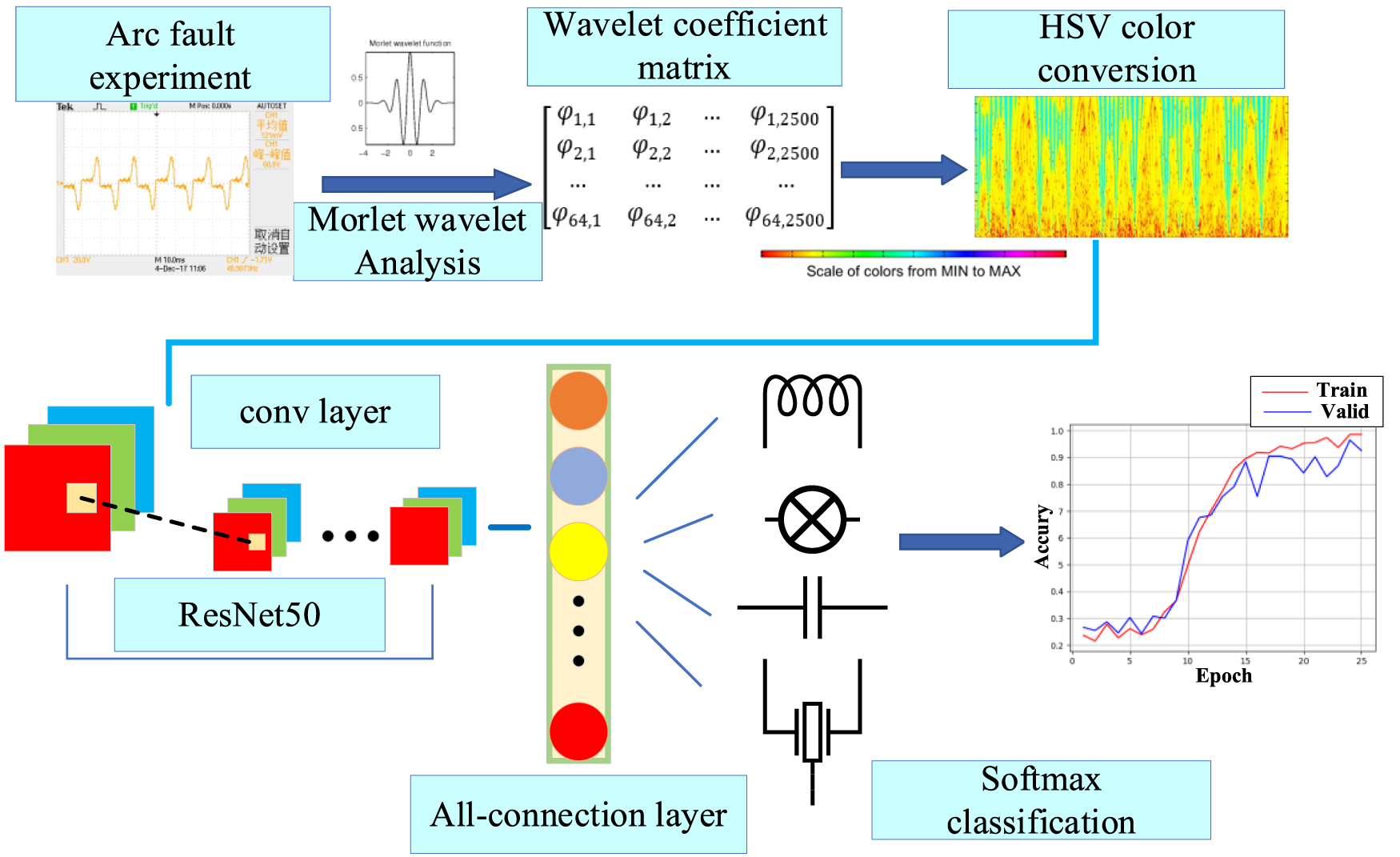
The process of arc fault detection method.
In Figure 1, the blue rectangle shows the specific content of the research steps, and the blue arrow shows the process of the research steps.
2 Experiment and data processing
In order to restore the real arc fault data, we set up an arc fault experiment platform according to the international standard UL1699. Six kinds of common loads in low-voltage circuits are connected with the arc fault generator in series. The sampling resistance method is used to measure the current time domain signals of six loads in normal working state and fault state. The load types and sampling resistance values are shown in Table 1.
TABLE 1
| Load name | Rated power (W) | The load type | The load properties | Sampling resistance(Ω) |
|---|---|---|---|---|
| Lamp | 100 | Resistive load | Linear load | 100 |
| Lamp and inductor in series | 100 | Resistive and inductive load | Linear load | 100 |
| Electric blower | 500 | DC motor load | Non-linear load | 50 |
| Induction cooker | 1200 | Eddy current load | Non-linear load | 1 |
| Computer | 90 | Switching power | Non-linear load | 50 |
| Hand drill | 500 | Series motor load | Non-linear load | 50 |
Load parameters and sample resistance values.
In 220 V, 50 HZ power grid environment, the six kinds of loads above are tested in normal operation and fault state for 4 times respectively. In the power grid, harmonics have little influence on the signal with the harmonic frequency higher than 20 times. In view of this, the sampling frequency of the experimental current is set as 25 KHZ according to Nyquist sampling theorem. Nyquist’s theorem can be expressed by Eq. 1:Where is the non-destructive sampling frequency and is the highest harmonic frequency of the time domain signal.
The 48 groups of data obtained from the experiment are reproduced in Matlab. Taking incandescent lamp and computer of linear load and non-linear load as examples respectively, which experimental results are shown in Figures 2, 3.
FIGURE 2
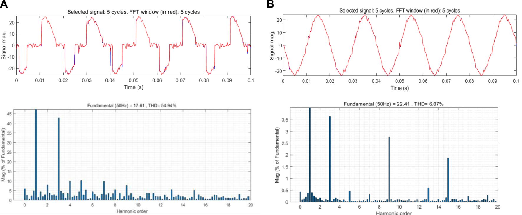
Experimental results, (A) is the time-frequency information under the failure of the incandescent lamp, (B) is the time-frequency information under the normal operation of the incandescent lamp.
FIGURE 3
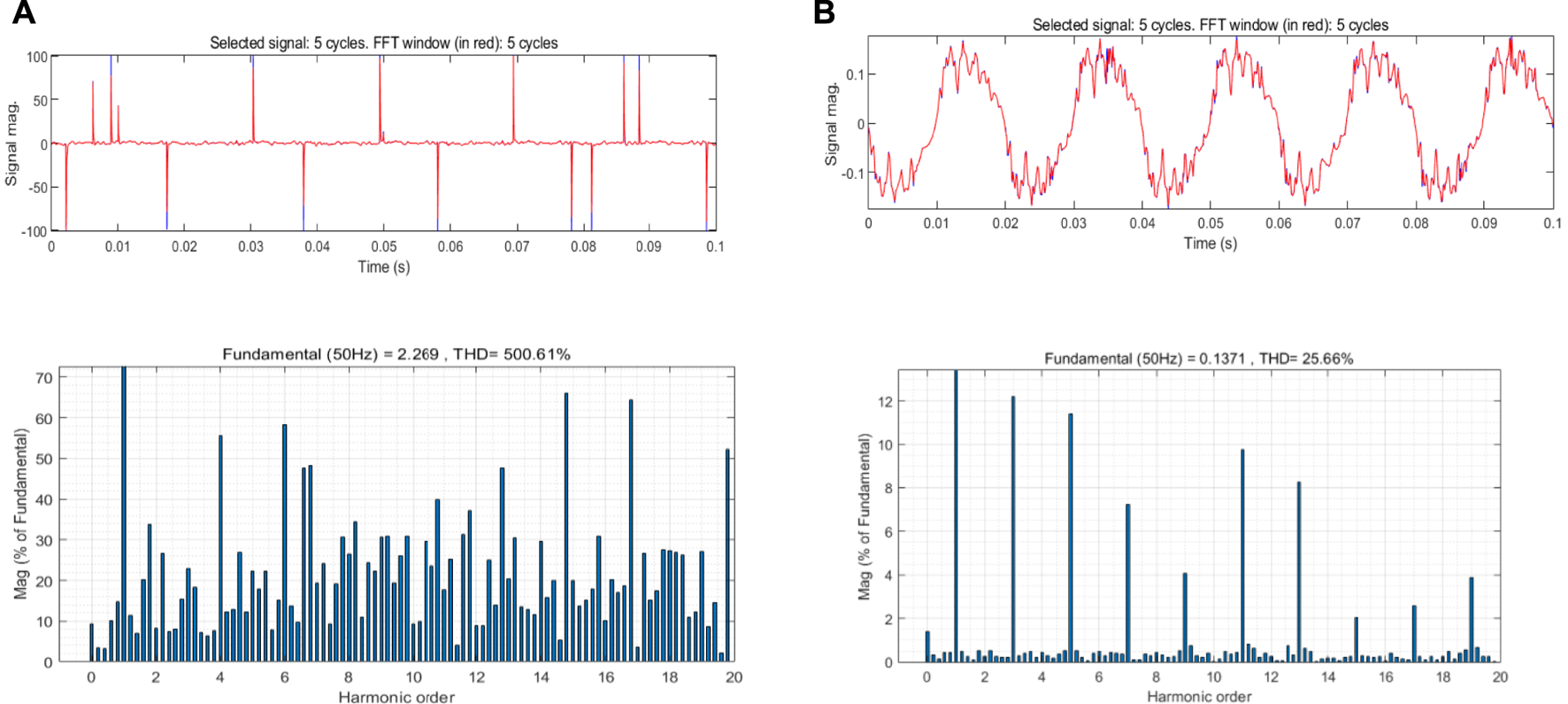
Experimental results, (A) is the time-frequency information under the failure of the computer, (B) is the time-frequency information under the normal operation of the computer.
The spectrum in the figure is obtained by fast Fourier analysis transform (FFT) of time-domain signals. It can be seen from the figure that the “flat shoulder” phenomenon occurs near the zero crossing of non-linear load when it fails. Ac arc in the current zero moment, the arc will automatically extinguished, and after the current zero, if the conditions are available, it will restart the arc. This phenomenon of the arc going out before and after the current crossing zero is known as the “zero-rest” of the AC arc. In the frequency spectrum, the linear load has a higher odd number of high harmonics during the failure. In addition, the total harmonic distortion (THD) rate reaches 54.94%, which is much higher than 6% under normal operation. By contrast, the time domain current of non-linear load presents high randomness, higher harmonic component and complete distortion of signal. In normal operation, the non-linear load also produces odd high order harmonics and the harmonic amplitude is higher than that of the linear load. In the research of arc faults, fault features are usually combined with machine learning algorithms to ensure the accuracy and rigor of detection (Johnson and Kang, 2012) (Cao et al., 2013).
3 Morlet continuous wavelet analysis
By using FFT, we can obtain the frequency domain distribution of the continuous signal over the sampling period. At the end of Section 2, we verify that the arc fault of non-linear load cannot be judged by spectrum alone. The fault features used for detection need deep fusion as well as generality and typicality. Wavelet analysis can be used to process the time domain signal. For the multi-resolution characteristic of wavelet function, continuous wavelet analysis can obtain the overall and detailed features of signal at different scales. 1D wavelets are mainly used to process ordinary 1D signals, while 2D wavelets are mainly used to process image signals. In addition, the cost of1d wavelet analysis is lower. Therefore, Morlet 1D wavelet, which is more suitable for 1D current signal in this paper, is selected. The continuous wavelet transform can be expressed as:
The meaning of Eq. 2 is as follows: After the mother wavelet ψ(t) is displaced by b, the inner product operation is carried out with the time domain signal f(t) at different scales a (Mallat and Zhong, 1992) (ByPaul, 2016). The “*” indicates that the complex conjugate of the wavelet function is used in the transform. In order to obtain more fault features at different scales, the typical Morlet continuous wavelet is selected to analyze the current signal (Ferracuti et al., 2021). The Morlet mother wavelet function is as follows:Where C is the approximate coefficient. The continuous wavelet transform is an integral transform, which is the same as the Fourier transform. The continuous wavelet transforms the mother wavelet by continuous translation and scaling, and then the wavelet coefficient is obtained. The wavelet coefficient is a binary function composed of translation and scaling, and the continuous wavelet transform can be expressed as:
The Morlet continuous wavelet transform coefficient can be expressed as:Where is the center frequency, a is the scale coefficient and b is the translation coefficient. The current time-domain signal obtained in the experiment was taken as the original signal for Morlet continuous wavelet analysis with the maximum scale of 64. Taking the incandescent lamp fault as an example, the wavelet coefficient with the change of time when the central scale a = 32 was shown in Figure 4:
FIGURE 4
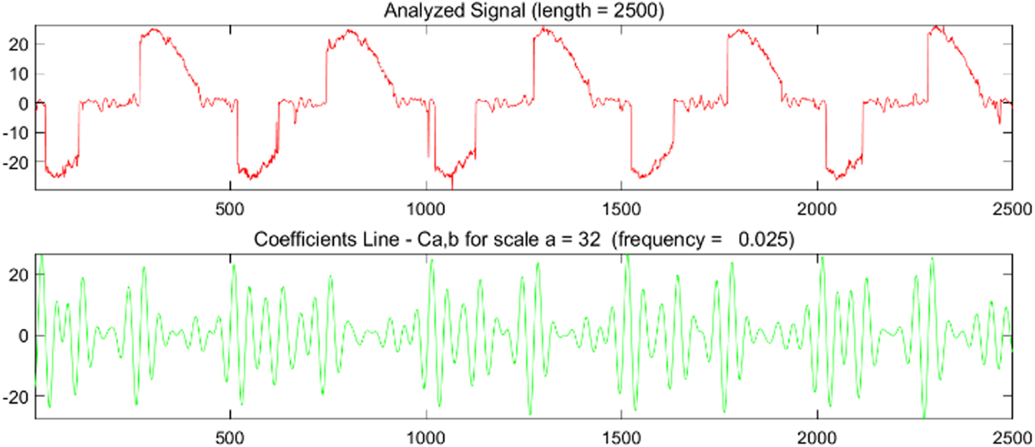
Original time domain signal and wavelet coefficient value curve of incandescent lamp fault.
Fusion of more features can improve the accuracy of the detection algorithm. In the next section, we try to use computer vision network to classify and detect fault features. Therefore, we try to transform fault features which fused with more scales into images. The wavelet coefficients obtained from each experiment are arranged into a 64 × 2500 matrix according to the scale of 1–64. The phase space depth diagram of continuous wavelet transform is made by mapping the coefficient matrix into the phase space of “hsv colormap”, as shown in Figure 5. The method of “Colormap index” works by mapping matrix values onto a preset colormap. One thing to note, Different from the familiar HSV-color mode, the “hsv colormap” in Matlab is also coded by RGB mode (Gonzalez, Woods) (Hartley and Zisserman, 2003). By using this method, the image is convolved in the form of three-channel (RGB) respectively. A wider receptive field can be obtained during the traversal operation of the convolution kernel (Morteza et al., 2021), thus achieving higher recognition accuracy.
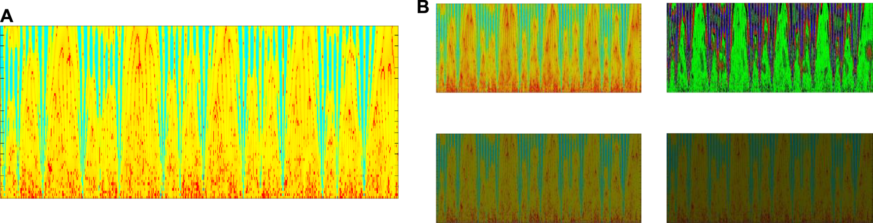
FIGURE 5
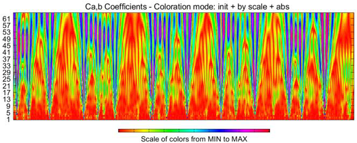
Depth map of phase space of continuous wavelet transform.
The significance of Figure 5 is that the color index at the bottom of the image represents the size of the wavelet coefficient from small to large. The horizontal axis is the sampling time axis, and the vertical axis is the scale axis. By adjusting the color value at the bottom of the image, the color domain of the phase space depth map can be changed to obtain different images. Figure 6 is the phase space map with the color domain changed. The above processing is applied to the data we obtained from 48 groups of experiments, and the 480 images are labeled artificially according to load types and working conditions. The data sets are set for subsequent classification detection. The use of “hsv colormap” will also be more convenient for the image enhancement method above.
FIGURE 6
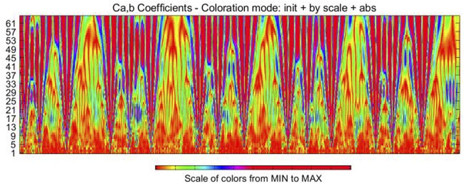
Phase space image of wavelet coefficients after changing color domain.
By this way, we obtain the time-frequency domain characteristics of arc faults at various scales. Image transformation can fuse features better and meet the requirements of subsequent neural networks for data dimension. In addition, compared with complex data features and matrix feature, graph features is more friendly to users without prior knowledge. In fact, wavelet analysis can be combined with control algorithm to achieve the purpose of optimizing performance in engineering field. For example, combining with particle swarm optimization algorithm to adjust the wavelet parameters and improve the performance of pattern recognition algorithm, or using Morlet wavelet function as the activation function of neural network to fit the parameters of robot travel (Dutta et al., 2013) (Vázquez et al., 2015). We attempt to improve the performance of neural networks for small sample datasets from the perspective of image feature engineering in the following sections.
4 ResNet50 arc detection model
Deeper convolutional neural networks can learn deeper data features. The identity mapping of neural networks between network layers is realized by updating network weights. The learning process of neural networks is the process of updating the weights between network layers through the back propagation of gradients between network layers (Amora et al., 2022). According to the chain derivative rule, gradient disappearance or gradient explosion will occur with the increase of neural network layers. Normalization of data can alleviate this phenomenon.
4.1 Batch-normalization
In order to prevent the simple linear relationship between the input and output of neural network neurons, we use ReLU as the activation function to add non-linearity to the neurons. The processed function can approximate any non-linear function. ReLU function can be expressed as Eq. 6:
For deep neural networks, the distribution of neuron input values will shift with the training process. The overall distribution will approach the extreme value of non-linear function generally. The addition of batch-normalization fixes the distribution of input values across layers to a standard normal distribution with an expectation of 0 and variance of 1 (Huang et al., 2021). One-hot labels are set for the four data sets, and 8 images in each sub-data set are used as mini-batch for training to improve training efficiency. Batch-normalization for input of neurons in layer K of neural network through input value X after activation function can be expressed as Eq. 6:Where, and are the expectation and variance of the whole data set, and the normalized result can be obtained through network parameters and changes:
Accordingly, the variance and expectation in Eq. 6 should be the unbiased estimation of corresponding statistics in the mini-batch composed of every 8 images.
4.2 ResNet50 network structure
ResNet is a typical model in the field of computer vision. The proposal of ResNet enables convolutional neural network to avoid network degradation even when the number of network layers increases to a large extent (Qu et al., 2019a). As we known, deep neural networks take multi-convolutional layers as parameter mapping. According to the chain rule, deep networks face the problem of gradient explosion or gradient disappearance when calculating gradients. The idea of ResNet is to make the deep network obtain the gradient of the shallow network through the mapping of residuals. When the input parameter X maps to H (X), the residual can be expressed as:
ResNet takes the residuals as a mapping. The input and output of the network layer are identical mappings even when gradient disappearance occurs, thus preventing the network performance degradation caused by gradient disappearance. In practical applications, the residual is usually not 0, so the network layer can learn new features from the input features to improve the accuracy of the network. The convolutional block structure of ResNet50 can be expressed in Figure 7.
FIGURE 7
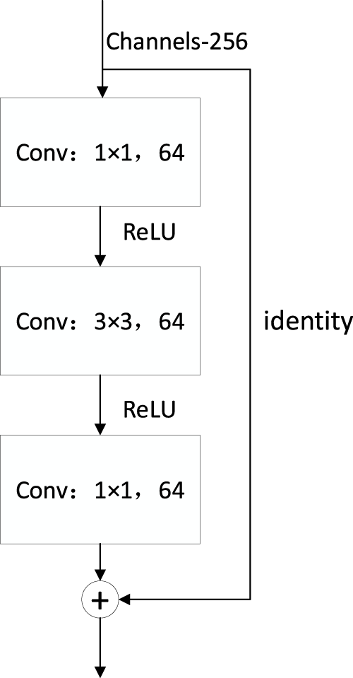
ResNet50 convolutional block structure.
ResNet can be expressed as the mathematical model shown in Eq. 10:Where x is the input vector, y is the output vector, and F is the residual mapping, which is part of network training. The convolutional Block in Figure 7 skips two layers, and its residual mapping can be expressed as:
We use different convolution kernels for convolution with step 2 and maximum pooling respectively, and then restore ResNet using convolution block as shown in Figure 7. Softmax layer is added in the output layer of the network to predict the type of feature and the maximum value is the prediction category. The specific model of the network is shown in Table 2:
TABLE 2
| Layer name | 50-layer |
|---|---|
| Conv1 | 7 × 7,6, stride 2 |
| Conv2_x | 3 × 3, max pool, stride 2 |
| Conv3_x | |
| Conv4_x | |
| Conv5_x | |
| average pool,1000-d fc, softmax |
ResNet50 detects network structure.
4.3 Implementation of the detection method
The process of arc fault detection can be summarized as the following steps:
1. The arc fault current data of different loads are obtained by experiments.
2. The fault features of 64 scales were obtained by Morlet wavelet analysis.
3. “Colormap index method” is used to convert numerical features into image features. Image data is preprocessed using data enhancement graph.
4. The fault dataset is put into ResNet50 for classification detection.
4.4 Classification and detection results of arc fault
The image data set is divided into training set and test set according to the ratio of 9:1, and the hyperparameters of the neural network are adjusted through repeated training so that the neural network can obtain higher classification accuracy. Since 480 images are relatively small image samples, Adam algorithm is added to dynamically adjust the learning rate of neural network in order to prevent the increase of loss caused by uneven distribution of image samples in each iteration. Hyperparameters are adjusted through several experiments. The pre-trained model with the highest accuracy is selected as the result. The final neural network hyperparameters are shown in Table 3.
TABLE 3
| Hyperparameter | Value |
|---|---|
| Image size | 100 × 100 |
| Batch size | 8 |
| Epoch | 20 |
| Target category | 4 |
Neural network training hyperparameters.
All the algorithms above are implemented based on Keras platform interface Tensorflow. The neural network is trained on Intel I7-9750H processor (8G RAM) and the graphics card is NVIDIA RTX 2060 (6G).
In order to reflect the changes in the accuracy of training set and validation set in each epoch during the training process, the average accuracy and loss changes in each epoch are made into curves, and the training results were shown in Figure 8.
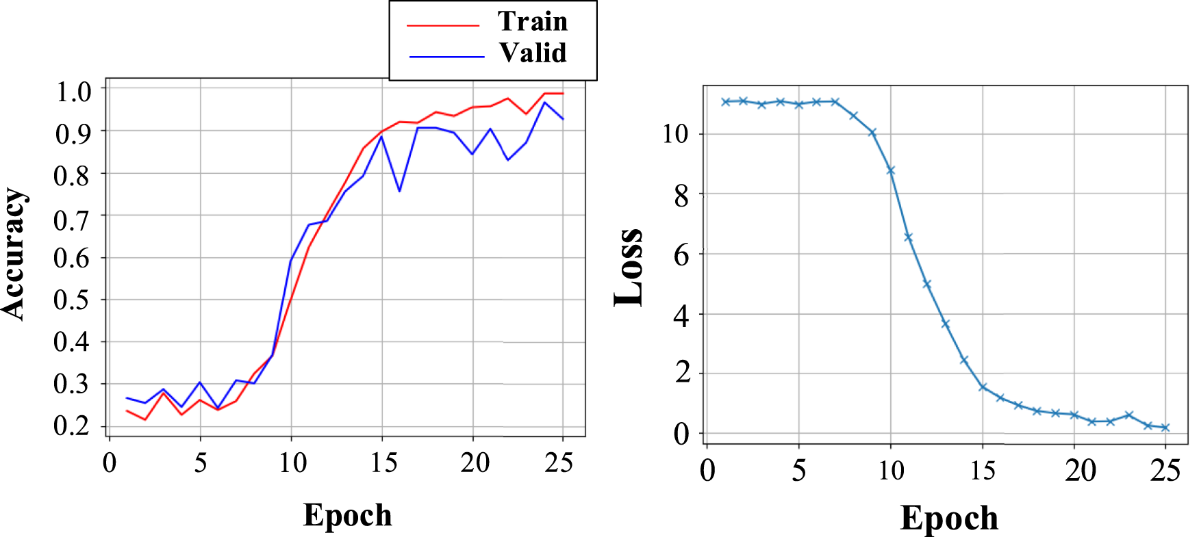
FIGURE 8
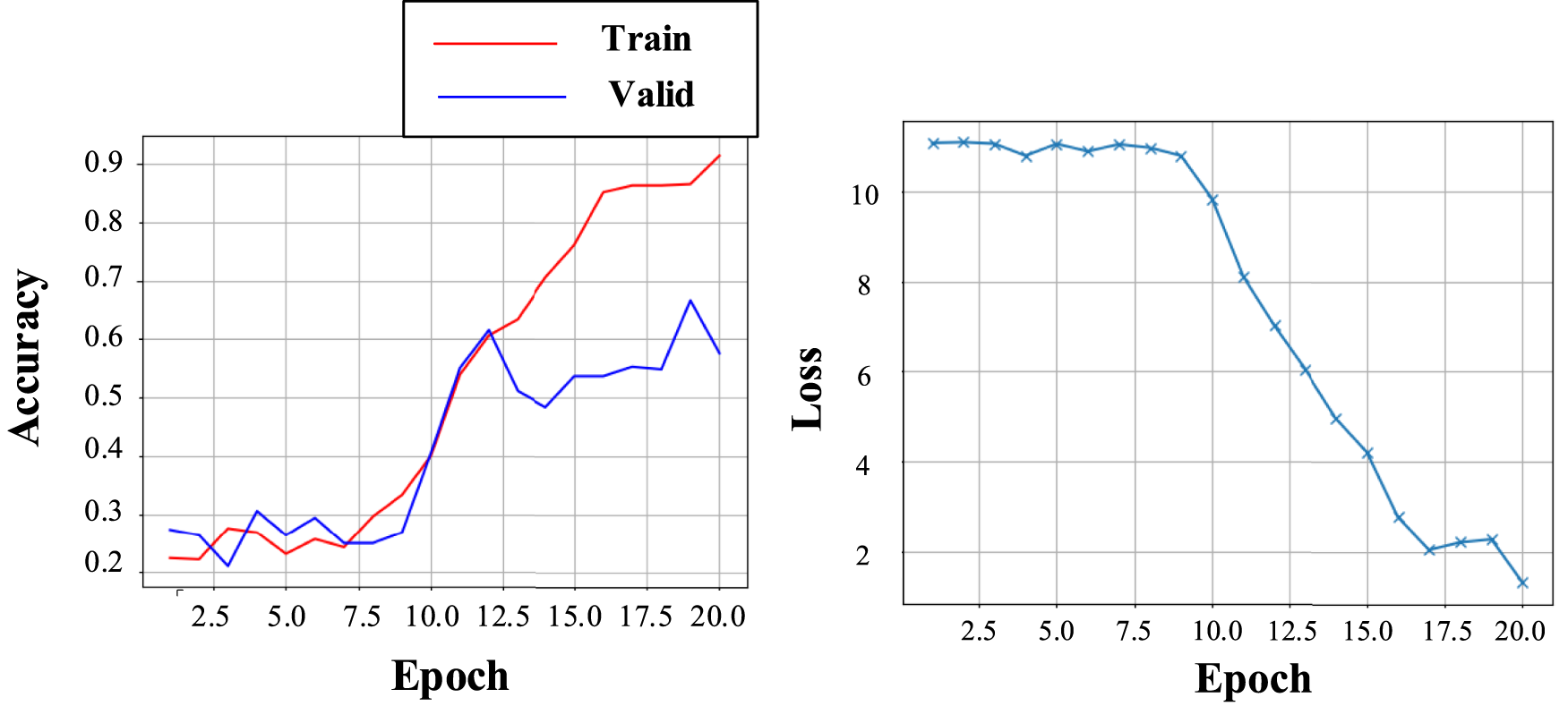
Training accuracy and loss curves of ResNet50.
The accuracy rate in the figure is the average of each epoch, and the image on the right is the change curve of the cross-entropy loss function.
In order to compare the training connection of the network, the accuracy of training set better, the accuracy of verification set and the loss value of epoch18-20 are expressed in numbers, as shown in Table 4:
TABLE 4
| layers | Epoch | Train accuracy (%) | Valid accuracy (%) | loss |
|---|---|---|---|---|
| 50 | 18 | 86.34 | 54.86 | 2.21 |
| 19 | 86.57 | 66.67 | 2.28 | |
| 20 | 91.43 | 57.64 | 1.31 |
ResNet50 training accuracy rate and loss change table.
As can be seen from Figure 8, the accuracy of the verification set began to be lower than that of the training set since the epoch is 11. When the epoch is 20, the accuracy of the training set still showed an upward trend, while the loss tended to converge. The accuracy of the verification set is 30% lower than that of the training set, which indicates that the network has a certain over-fitting phenomenon. Due to the small number of samples in the dataset and the image data obtained through color domain transformation, many images may have certain similarity. Insufficient sparsity of data samples may lead to uneven distribution of samples.
5 Image data enhancement
5.1 Image preprocessing
Neural networks achieve the purpose of classification by fitting the distribution of the training dataset. Suppose the data distribution P (x, y) is known, where x is the feature, y is the label, Given a specific loss function (⋅), for a model assuming h∈ . We expect a machine learning algorithm to minimize its expected risk, which is defined as Eq. 12.
In fact, the data distribution P (x, y) is usually unknown, so it is difficult to be integrated. Propose that the number of samples with labels is I. We approximate this distribution with the sampling results, and seek to minimize the empirical risk. Here, “experience” means the data set obtained by sampling. Eq. 12 can be rewritten as Eq. 13
The parameter h can be represented in the following ways:Where is the theoretical assumption optimal value. Because the data distribution of the sample set is unknown, the value of cannot be found.Where is the constraint value assumed to minimize the expected risk in the data space .
This equation represents the optimal hypothesis obtained by optimizing on a specified data set of amount I and minimizing the empirical risk under the specified hypothesis space h∈ .
Two error forms of the assumed distribution and the actual distribution can be obtained through the three equations above.
Where
denotes the difference between the optimal solution
of the hypothetical space
and the ideal value
under the expected loss.
represents the error between the data sample and the assumed data distribution. The performance of the network can be improved by reducing the above errors. When the amount of training data increases, the neural network will get more supervision information.
can approximates
better (
Wang et al., 2019) (
Zhang et al., 2021). The performance of the network can be improved by reducing the above errors. In order to solve the problem of neural network overfitting caused by small sample data sets. We used the following two kinds of non-linear image transformation methods to amplify the dataset.
1) Random gamma variation of the image
Gamma change is also known as the curve gray change of color image. In the field of image processing, gamma change of image is often used to adjust the contrast. Gamma change is a non-linear change acting on pixel gray value, which can be expressed mathematically as Eq.
18:
Where,
Sis the gray value after gamma changes, and
Cis the gray scale coefficient, which is 1 in this paper. “
r” is the gray value of the image input, and its value range is [0,1].
is the gamma influence factor, we change the value of gamma randomly to amplify the original image. When the gamma value is greater than 1, the area of the image with lower gray value will be stretched, and the part with higher gray value will be compressed. For gamma values less than 1, the reverse action is performed. The image is converted to grayscale image to make the subsequent image computation less. The description of gray image, like color image, still reflects the distribution and characteristics of the overall and local chromaticity and highlight level of the whole image. The images after gamma changes are shown in
Figure 9.
2) Random rotation of the image
FIGURE 9
Gamma change of the image, (A) is the original image, and (B) is the image after gamma change.
Rotate the image at random Angle without changing the size of the image. Fill the free part of the rotation with black and the images after random Angle rotation are shown in Figure 10.
FIGURE 10
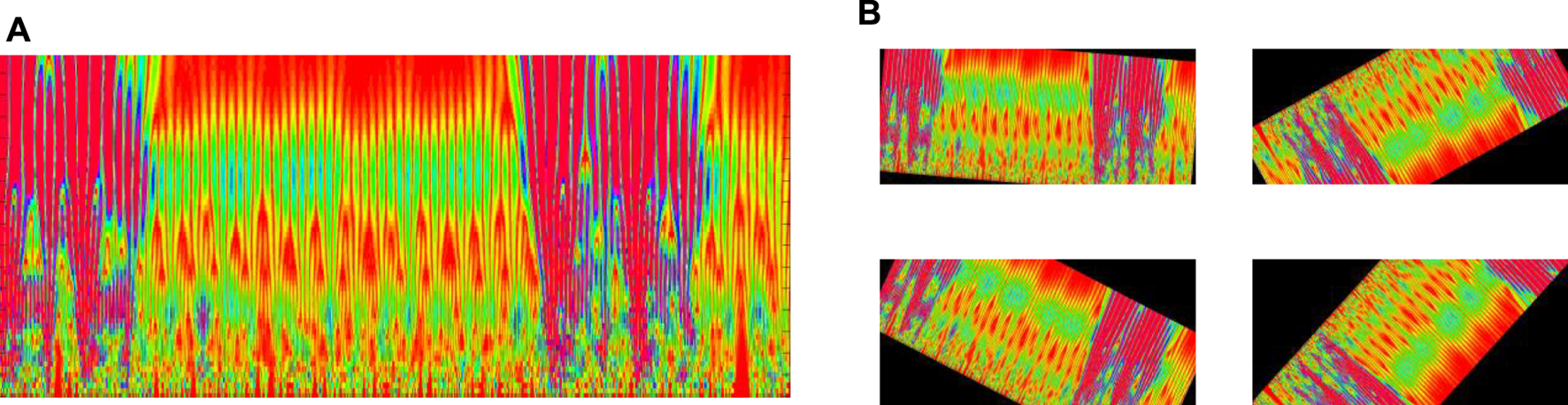
Random Angle changes of the image, (A) is the original image, (B) is the changed image.
The original image is changed by the above two methods, and 5 new images are obtained for each image. The new dataset contains 960 images, which is two times the size of the original dataset.
5.2 Network training results after data enhancement
On the basis of not changing epoch and mini-Batch parameters, we use the enhanced data set to conduct neural network training of ResNet50. After training, the average accuracy and average loss of the training set and verification set on each epoch are shown in Figure 11:
FIGURE 11
ResNet50 training results after data enhancement.
When the epoch is 23–25, the classification training results of neural network can be expressed in Table 5:
TABLE 5
| layers | Epoch | Train accuracy (%) | Valid accuracy (%) | loss |
|---|---|---|---|---|
| 50 | 23 | 93.75 | 87.04 | 0.60 |
| 24 | 98.61 | 96.53 | 0.25 | |
| 25 | 98.61 | 92.59 | 0.18 |
ResNet50 classification training results after data enhancement.
It can be seen that the over-fitting phenomenon of neural network is solved after adding data enhancement to the data set. The network obtained the highest accuracy of validation set and training set when the epoch is 24. Compared with Table 4, the loss value of the neural network is generally lower, indicating that the neural network had learned more image features and the preprocessing of the data set is effective (Li et al., 2021) (Qu et al., 2019b).
5.3 The comparison experiment
We set up a comparison method to verify the detection performance of ResNet50. In addition, we consider verifying whether our proposed method is suitable for classical lightweight networks including AlxNet, InceptionV4 and VGG19. The image data enhancement method also applied in the comparing methods. To ensure convergence of the loss function, we increased the hyperparameter epoch in the comparison test to 50. However, other neural networks showed serious overfitting phenomenon. Hence the “early stop” has been carried out. The network pre-training results are shown in Table 6.
TABLE 6
| Network | Train accuracy (%) | Valid accuracy (%) | loss |
|---|---|---|---|
| ResNet50 | 98.61 | 96.53 | 0.25 |
| AlxNet | 24.77 | 12.5 | 11.09 |
| InceptionV4 | 23.84 | 28.47 | 11.12 |
| VGG19 | 24.68 | 12.5 | 11.09 |
Other typical computer vision network pre-training results.
It can be seen that the accuracy of other typical networks is maintained at 20%–30%. The loss function stays around 11 which suggests that the network is not learning the deeper features of the image. Due to the limitation of the fault conditions, it is difficult to obtain large numbers of fault samples. Compared with ResNet, the visual model above is prone to the problem of gradient disappearance/explosion when dealing with small samples and similar data.
6 Conclusion
This paper presents a series arc fault detection method combining Morlet wavelet analysis and computer vision. Common load arc fault current is sampled by sampling resistance method. The Morlet wavelet with the scale of 64 is applied to deep fault feature fusion.
The matrix composed of wavelet coefficients is mapped to images by HSV color index. The image data is used as the feature to establish the detection data set, and the data categories are annotated manually. ResNet50 is applied to feature image recognition. In addition, we propose a data enhancement method of image random gamma transform and random rotation. Experimental results show that data enhancement can effectively improve the over-fitting phenomenon of neural network, and improve the detection accuracy to 96.53%.
It is worth mentioning that the image feature extraction in this paper provides a new method for feature selection. More researches can be done on image features, such as dimensionality reduction of image level data, image preprocessing that can change network performance, and image expression of typical network regularization.
Computer vision has brought a lot of convenience to our life. Just like face recognition, we look forward to applying computer vision to fault arc detection.
Statements
Data availability statement
The original contributions presented in the study are included in the article/supplementary material, further inquiries can be directed to the corresponding author.
Author contributions
ZS is responsible for the main body of the article NQ a is responsible for directing the experiment CH and TZ are responsible for the revision and data processing of the article.
Funding
This work is supported in part by the National Natural Science Foundation of China under Grant 61901283 and National Natural Science Foundation of China (Grant No 62003080, U22A2055, 62273058), and the Fundamental Research Funds for the Central Universities (Grant No N2204011).
Conflict of interest
The authors declare that the research was conducted in the absence of any commercial or financial relationships that could be construed as a potential conflict of interest.
Publisher’s note
All claims expressed in this article are solely those of the authors and do not necessarily represent those of their affiliated organizations, or those of the publisher, the editors and the reviewers. Any product that may be evaluated in this article, or claim that may be made by its manufacturer, is not guaranteed or endorsed by the publisher.
Abbreviations
, Non-destructive sampling frequency; , Variance; , Highest harmonic frequency; (⋅), Specific loss function; ψ(t), The mother wavelet; , Theoretical assumption optimal value; f(t), Time domain signal; , Constraint value; C, Approximate coefficient; S, Gray value; , Center frequency; γ, Gamma influence factor; A, Scale coefficient; B, Translation coefficient; , Expectation.
References
1
Amora D. J. A. Deocadiz A. B. Sañejo G. L. Santiago C. J. R. Umali M. G. Arenas S. U. (2022). “NPK prediction based on pH colorimetry utilizing ResNet for fertilizer recommender system,” in IET International Conference on Engineering Technologies and Applications, Changhua Taiwan, 14-16 October 2022(IET-ICETA), 1–2. 10.1109/IET-ICETA56553.2022.9971508
2
ByPaul S. A. (2016). The illustrated wavelet transform handbook introductory theory and applications in science, engineering, medicine and finance, Boca Raton: CRC Press, 978.
3
Cao Y. Li J. Sumner M. Christopher E. Thomas D. (2013). “Arc fault generation and detection in DC systems,” in IEEE PES Asia-Pacific Power and Energy Engineering Conference, Hong Kong, 08-11 December 2013(APPEEC), 1–5. 10.1109/APPEEC.2013.6837123
4
Chen H. Gan Z. Yang H. (2014). “Realizing speech enhancement by combining EEMD and K-SVD dictionary training algorithm,” in The 9th International Symposium on Chinese Spoken Language Processing, Singapore, 12-14 Sept. 2014(IEEE), 378.
5
Chu R. Schweitzer P. Zhang R. (2020). Series AC arc fault detection method based on high-frequency coupling sensor and convolution neural network. Sensors20 (17), 4910. 10.3390/s20174910
6
Cui R. Li Z. (2021). arc fault detection and classification based on three-dimensional entropy distance and EntropySpace in aviation power system[J]. Trans. China Electrotech. Soc.36 (04), 869–880. 10.19595/j.cnki.1000-6753.tces.191717
7
Cui R. Li Z (2021)arc fault detection based on phase space reconstruction and principal component analysis in aviation power system. Trans. China Electrotech. Soc.41(14):5054–5065. 10.13334/j.0258-8013.pcsee.201323
8
Cui R. Tong D. (2021). Frequency domain analysis and feature extraction of aviation AC arc fault and crosstalk[j]. Electr. Mach. Control25 (06), 18–26. 10.15938/j.emc.2021.06.003
9
De P. Chatterjee A. Rakshit A. (2021). Regularized K-SVD-Based dictionary learning approaches for PIR sensor-based detection of human movement direction. IEEE Sensors J.21 (5), 6459–6467. 10.1109/jsen.2020.3040228
10
Dutta S. Pal S. K. Mukhopadhyay S. Sen R. (2013). Application of digital image processing in tool condition monitoring: A review. CIRP J. Manuf. Sci. Technol.6, 212–232. 10.1016/j.cirpj.2013.02.005
11
Ferracuti F. Schweitzer P. Monteriù A. (2021). Arc fault detection and appliances classification in AC home electrical networks using recurrence quantification plots and image analysis. Electr. Power Syst. Res.201, 107503. 10.1016/j.epsr.2021.107503
12
Gonzalez R. C. Woods R. E. (2021). Digital image processing. second edition. Upper Saddle River, New Jersey, United States: Prentice-Hall. 7-5053-7798.
13
Hartley R. Zisserman A. (2003). Multiple view geometry in computer vision. Cambridge: Cambridge University Press, 655.
14
Huang G. Qiao L. Khanna S. Pavlovich P. A. Tiwari S. (2021). Research on fan vibration fault diagnosis based on image recognition. J. Vibroengineering23 (6), 1366–1382. 10.21595/jve.2021.21935
15
Humbert J. B. Schweitzer P. Weber S. (2021). Serial-arc detection by use of Spectral Dispersion Index (SDI) analysis in a low-voltage network (270V HVDC) [J]. Electr. Power Syst. Res.196, 107084.10.1016/j.epsr.2021.107084
16
Ji H. Kim S. GyungSuk K. (2020). Phase analysis of series arc signals for low-voltage electrical devices. Energies13 (20), 5481. 10.3390/en13205481
17
Joga S. R. K. Sinha P. Maharana M. K. (2021). Performance study of various machine learning classifiers for arc fault detection in AC microgrid. IOP Conf. Ser. Mater. Sci. Eng.1131 (1), 012012. 10.1088/1757-899x/1131/1/012012
18
Johnson J. Kang J. (2012). “Arc-fault detector algorithm evaluation method utilizing prerecorded arcing signatures,” in 38th IEEE Photovoltaic Specialists Conference, Austin, TX, USA, 03-08 June 2012, 001378–001382. 10.1109/PVSC.2012.6317856
19
Kadian P. Arora N. Arora S. M. (2019). “Performance evaluation of robust watermarking using DWT-SVD and RDWT-SVD,” in 6th International Conference on Signal Processing and Integrated Networks (SPIN), Noida, 07-08 March 2019, 987–991.
20
Ku W. Storer R. H. Georgakis C. (1995). Disturbance detection and isolation by dynamic principal component analysis. Chem. Intel. Lab. Syst.30 (1), 179–196. 10.1016/0169-7439(95)00076-3
21
Lala H. Subrata K. (2020). Classification of arc fault between broken conductor and high‐impedance surface: An empirical mode decomposition and stockwell transform‐based approach. Transm. Distribution14 (22), 5277–5286. 10.1049/iet-gtd.2020.0340
22
Li B. Zhang Z. Duan F. Yang Z. Zhao Q. Sun Z. et al (2021). Component-mixing strategy: A decomposition-based data augmentation algorithm for motor imagery signals. Neurocomputing465, 325–335. 10.1016/j.neucom.2021.08.119
23
Liu G. Du S. (2017). Research on LV arc fault protection and its development trends. Power Syst. Technol.41 (01), 305–313. 10.13335/j.1000-3673.pst.2016.0804
24
Lu S. Rui M. Phung T. Tharmakulasingam S. Daming Z. et al (2021). Lightweight transfer nets and adversarial data augmentation for photovoltaic series arc fault detection with limited fault data[J]. Int. J. Electr. Power Energy Syst.130, 107035. 10.1016/j.ijepes.2021.107035
25
Mallat S. Zhong S. (1992). Characterization of signals from multiscale edges. IEEE Trans. Pattern Analysis Mach. Intell.14 (7), 710–732. 10.1109/34.142909
26
Miao W. Wang Z. Wang F. Lam K. H. Pong P. W. T. (2023). Multicharacteristics Arc model and autocorrelation-algorithm based arc fault detector for DC microgrid. IEEE Trans. Industrial Electron.70 (5), 4875–4886. 10.1109/TIE.2022.3186351
27
Morteza S. Samir K. Mohammad-Hadi P. Ramazan-Ali J-T. et al (2021). Damage detection on rectangular laminated composite plates using wavelet based convolutional neural network technique. Compos. Struct.278, 114656. 10.1016/j.compstruct.2021.114656
28
Qu N Wang J. (2018). A series arc fault detection method based on Cassie model and L3/4 norm[J]. Power Syst. Technol.42 (12), 3992–3997. 10.13335/j.1000-3673.pst.2017.3091
29
Qu N. Wang J. Liu J. (2019). An Arc fault detection method based on current amplitude spectrum and sparse representation. IEEE Trans. Instrum. Meas.68 (10), 3785–3792. Response to the editor and reviewer. 10.1109/tim.2018.2880939
30
Qu N Zuo J. Chen J. (2019). Series Arc fault detection of indoor power distribution system based on LVQ-NN and PSO-SVM[J]. IEEE Access2019(7), 184019–184027. 10.1109/ACCESS.2019.2960512
31
Shu L. Wang P. (2018). Study on dynamic circuit model of DC icing flashover based on improved time-varying arc equation[J]. Trans. China Electrotech. Soc.33 (19), 4603–4610. 10.19595/j.cnki.1000-6753.tces.171391
32
Vázquez L. A. Jurado F. Alanís A. Y. (2015). Decentralized identification and control in real-time of a robot manipulator via recurrent wavelet first-order neural network. Math. Problems Eng.451049, 1–12. 10.1155/2015/451049
33
Vozalis M. G. Margaritis K. G. (2006). Applying SVD on generalized item-based filtering. IJCSA3 (3), 27–51.
34
Wang L Qiu H. Yang P. (2021). arc fault detection algorithm based on variational mode decomposition and improved multi-scale fuzzy entropy. Energies14 (14), 4137. 10.3390/en14144137
35
Wang Y. Yao Q. Kwok J. (2019). Generalizing from a few examples: A survey on few-shot learning,//arXiv: 1904.05046.
36
Xia Z. Chen Y. Xu C. (2022). Multiview PCA: A methodology of feature extraction and dimension reduction for high-order data. IEEE Trans. Cybern.52, 11068–11080. 10.1109/tcyb.2021.3106485
37
Xiang C. Wang H. (2019). Research on the combustion process of vacuum arc based on an improved pulse coupled neural network model[J]. Trans. China Electrotech. Soc.34 (19), 4028–4037. 10.19595/j.cnki.1000-6753.tces.181158
38
Xiong Q. Chen W. (2020). Review of research progress on characteristics, detection and localization approaches of fault arc in low voltage DC system. Proc. CSEE[j]40 (18), 6015–6027. 10.13334/j.0258-8013.pcsee.200330
39
Zhang C. Xia K. Feng H. Yang Y. Du X. (2021). Tree species classification using deep learning and RGB optical images obtained by an unmanned aerial vehicle. J. For. Res.32 (05), 1879–1888. 10.1007/s11676-020-01245-0
40
Zhao H. Qin H. , A series fault arc detection method based on the fusion of correlation theory and zero current feature. 2020,41(04):218–228. 10.19650/j.cnki.cjsi.J2006019
Summary
Keywords
morlet continuous wavelet, arc fault, ResNet, regularization, color index
Citation
Shuai Z, Qu N, Zheng T, Hu C and Lu S (2023) Research on arc fault detection using ResNet and gamma transform regularization. Front. Energy Res. 11:1069119. doi: 10.3389/fenrg.2023.1069119
Received
13 October 2022
Accepted
07 February 2023
Published
17 February 2023
Volume
11 - 2023
Edited by
Srete Nikolovski, Josip Juraj Strossmayer University of Osijek, Croatia
Reviewed by
Arturo García Pérez, University of Guanajuato, Mexico
Sherif S. M. Ghoneim, Taif University, Saudi Arabia
Updates
Copyright
© 2023 Shuai, Qu, Zheng, Hu and Lu.
This is an open-access article distributed under the terms of the Creative Commons Attribution License (CC BY). The use, distribution or reproduction in other forums is permitted, provided the original author(s) and the copyright owner(s) are credited and that the original publication in this journal is cited, in accordance with accepted academic practice. No use, distribution or reproduction is permitted which does not comply with these terms.
*Correspondence: Na Qu, 11502332@qq.com
This article was submitted to Smart Grids, a section of the journal Frontiers in Energy Research
Disclaimer
All claims expressed in this article are solely those of the authors and do not necessarily represent those of their affiliated organizations, or those of the publisher, the editors and the reviewers. Any product that may be evaluated in this article or claim that may be made by its manufacturer is not guaranteed or endorsed by the publisher.