An accurate and efficient quasi-dynamic simulation method of electricity-heat multi-energy systems

Quasi-dynamic energy flow computation (EFC) has become a critical tool to determine and predict the states of the multi-energy system (MES), which helps improve MES’ operation efficiency and issues the security warning. However, methods in literature suffer numerical problems including fake oscillations, divergence, etc., Also, with the increasing of system dimensions, the computation efficiency can be hardly guaranteed due to the cross iterations between different nonlinear equations. This paper proposes an accurate and efficient method for quasi-dynamic energy flow computation. Using a scheme with total variation decreasing property, the numerical instability in solutions of thermal dynamics are effectively reduced. By estimating local truncation errors in a cheap way, the simulation step sizes are controlled adaptively and hence the overall simulation efficiency is greatly increased. Numerical tests were performed in a small system and the famous Barry Island system, which verified the advantages of the proposed method in both efficiency and accuracy.

1 Introduction

Nowadays, the wide exploitation of fossil fuels has apparently promoted the greenhouse effect. In view of this, the concept of multi-energy systems (MES) has been proposed to increase the overall energy utilization efficiency by reconciling the electric power with the more flexible heating power (Zhang M. et al., 2021; Jiang et al., 2021; Li et al., 2021; Zheng et al., 2022). However, the heterogenous forms of energy, which are depicted by disparate mathematical models, complicate the underlying operational law of MES. Several analysis methods have been put forward in literature to tackle this, including the steady-state energy flow computation (EFC) (Liu et al., 2016; Zhang et al., 2021b; Li et al., 2022), the quasi-dynamic EFC (Pan et al., 2016; Qin et al., 2019; Yao et al., 2021; Yu et al., 2022; Zhang et al., 2022) and the combined dynamic simulation (Shen et al., 2020; Wang et al., 2022). Among these methods, the quasi-dynamic EFC can plot the temperature variations precisely while demonstrates moderate modelling complexity, which has drawn much attention.

Essentially, the quasi-dynamic EFC in MESs is to simulate the spatio-temporal temperature distributions along pipelines, the variable mass flow rates, and the node temperature/power variations in heating network (HN) side, and the time-evolution of active/reactive power, and the voltage in power grid (PG) side. However, this becomes a non-trivial task when considering the spatial dimension of the system. Spatial evolution is a crucial feature that accounts for the time-delaying characteristics and hence flexibility of HN, but it cannot be modelled by ordinary differential equations. As a result, some mature and commercial time-domain simulation methods are inapplicable here. Recently, several efforts have been made in this area but are far from satisfactory. The developed methods undergo the influences of the so-called dissipative and dispersive errors, fail to respond quickly, and sometimes even diverges due to the numerical instability. Therefore, the development of a quasi-dynamic EFC method that possesses both fast responding time and high accuracy is still of great necessity.

The research gaps are summarized from two aspects in what follows. The first aspect is about the modelling and solutions of the spatio-temporal thermal dynamics in pipelines, which mainly falls into two categories: 1) the node method and 2) the partial differential equations (PDEs) and the related finite-difference/analytical methods. The node method is more physically sensible. It divides the whole pipelines into thermally insulated water masses, whose marching along the pipelines constitutes the thermal transmission. And the average temperatures of the water masses in the outlet buffer acts as the output temperatures (Li et al., 2016; 2023). Chen et al. have further proposed an enhanced node method, the water mass method, to eliminate the integer variables in optimization applications (Chen et al., 2019), which sheds light on the more complicated hydraulic-thermal cooperative operation optimization of MESs (Lu et al., 2020). It has been pointed out by Yu et al. that the node method is fairly accurate when depicting thermal dynamics but also suffer non-convergence issues in variable mass flow scenarios (Yu et al., 2022).

The PDEs are a more mathematical description of thermal dynamics. Some people discretize the spatial and temporal derivatives in the PDEs respectively to derive solvable algebraic constraints. Wang et al. have compared the accuracy and efficiency of the implicit upwind method and the characteristic line methods (Wang et al., 2017). Yao et al. have proposed a novel central scheme with unconditionally stability (Yao et al., 2021) But the fake oscillations and damping in the PDE solutions, which are called dispersive and dissipative errors respectively, are ignored in their works. By assuming constant mass flow, the analytical solutions of the PDE can be derived easily. Chen et al. (Chen et al., 2021) have used the Fourier analysis to derive a series solution. Yang et al. have derived the analytical power and temperature expressions with respect to boundary conditions of the PDE (Yang et al., 2020). And the initial condition case has been later finished by Zhang et al. (Zhang et al., 2022). Those analytical methods get rid of dispersive and dissipative errors completely but are not generic since the hydraulics are assumed to be still.

The second aspect is about how to obtain the time-varying hydraulics and electric variables, which are implicitly constrained by nonlinear algebraic equations. Qin et al. have proposed to alternatively solve the discretized PDEs and the remaining algebraic constraints (Qin et al., 2019). The PDE solutions first predict the thermal variables on the next time window, and then the remaining variables can be solved by Newton method accordingly. Yao et al. have pointed out the interaction errors between electric and heating variables and proposed the power-energy interfaces to calibrate the computation results (Yao et al., 2022). The cross iterations between PG and HN part of equations are computationally intensive, which hold up the responding time of energy flow analysis. Zhang et al. have proposed to uncouple the HN into sub-networks, which reduces the overall solution complexity and works well in constant mass flow scenarios (Zhang et al., 2021c). Huang et al. have applied the Levenberg-Marquardt-form Newton method to improve the convergence and efficiency of EFC (Huang et al., 2023). Yu et al. have proposed to derive time polynomials, which are called semi-analytical solutions, of unknown variables with a differential-transformation-based method (Yu et al., 2022). An adaptive time window strategy has also been developed to speed up the quasi-dynamic EFC and ensure convergence. However, the adaptive time window strategy of finite difference-based method has not been found in literature.

The research gaps are summarized as follows. The node method is physically sensible and accurate but is numerically unstable. The analytical methods provide exact solutions but are restricted to constant mass flow scenarios. The finite-difference-based methods are severely affected by the dissipative and dispersive errors, and the cross iterations between PG and HN sides are time-consuming. Also, some works focus on the HN side and overlook the interactions between PG and HN.

To overcome these limitations, this paper proposes a novel accurate and efficient solution method of quasi-dynamic EFC of MESs considering variable mass flow. The proposed method is based on the finite difference method, which is a flux limiter scheme with total variation decreasing (TVD) property. A novel expedite technique is further developed to accelerate the calculation. More precisely, the paper makes the following contributions:

1) The proposed method uses a flux limiter scheme to discretize the PDEs governing thermal dynamics, which effectively reduces the dispersive and dissipative errors.

2) The proposed method expedites the MES quasi-dynamic EFC by controlling the temporal simulation step size adaptively. The technique utilizes two different schemes to generate the local truncation error estimation, but the computation cost is cheap.

The structure of the paper is organized in the following way: Section 2 establishes the quasi-dynamic MES model; Section 3 introduces the flux limiter scheme of PDEs; Section 4 develops the expedite scheme; Section 5 gives the detailed simulation procedure; Section 6 gives the case studies; Section 7 concludes.

2 Model formulation

2.1 Thermal transmission equations

The thermal dynamics of the heating pipelines can be depicted by

$\frac{\partial T}{\partial t}+\frac{\dot{m}}{S\rho }\frac{\partial T}{\partial x}+\frac{1}{S\rho cR}\left(T-T^{\text{o}}\right)=0(1)$

where we denote by T (°C) the temporal-spatial distribution of temperatures along the pipelines; $\dot{m}$ (kg s⁻¹) is the mass flow rate; S (m²) is the cross-sectional area of the heating pipeline; ρ (kg m⁻³) is the density of mass flow; R (W m⁻¹ C⁻¹) is the thermal resistance of the pipeline segment; c (J kg⁻¹ C⁻¹) is the specific heat capacity; t and x are the time and position variables respectively; T^o (°C) is the outside temperature of pipeline.

2.2 Thermal equations

The node temperatures are the mixture of the outlet temperatures of the pipelines flowing into the node, which has the formula

$\sum m_i{T}_i^{\text{out}}=T_n\sum m_i,i\in {\mathbb{E}}_n^{\text{in}}(2)$

$T_i^{\text{in}}=T_n,i\in {\mathbb{E}}_n^{\text{out}}(3)$

where we denote by $T_i^{\text{out}}$/$T_i^{\text{in}}$ the outlet/inlet temperature of pipeline i; T_n is the temperature of node n; ${\dot{m}}_i$ is the mass flow rate of pipeline i; ${\mathbb{E}}_n^{\text{in}}/E_n^{\text{out}}$ is the set of pipelines flowing into/out of node n.

2.3 Hydraulic equations

The hydraulic models are comprised of the mass flow injection/continuity equation, which have the formula

$\sum _{j\in {\mathbb{E}}_n^{\text{in}}}{\dot{m}}_j=m_n^{\text{in}}(4)$

$\sum _{j\in {\mathbb{E}}_n^{\text{in}}}{\dot{m}}_j=\sum _{i\in {\mathbb{E}}_n^{\text{out}}}{\dot{m}}_i(5)$

where ${\dot{m}}_n^{\text{in}}$ is the node injection mass flow rate of node n.

Some HN contains loops and the pressure drop around a closed loop equals zero, so we have

$\sum _i{K}_i|{\dot{m}}_i|{\dot{m}}_i=0,i\in {\mathbb{E}}_j^{\text{loop}},j=\mathrm{1,2},\cdots (6)$

where we denote by K_i the resistance coefficients of pipe i. ${\mathbb{E}}_j^{\text{loop}}$ denotes the set of pipes in loop j.

2.4 Heating power equation

The heating power exchanged at a node can be computed as

$\varphi =c\left|{\dot{m}}^{\text{in}}\right|\left(T^{\text{s}}-T^{\text{r}}\right)(7)$

where we denote by ϕ the heating power, T^s and T^r are respectively the supply and return temperatures of the node.

2.5 Power flow equations of PG

Since the transients in PG are usually omitted in quasi-dynamic analysis (Qin et al., 2019; Zhang et al., 2022), we adopt the AC power flow equation

$\left\{\begin{array}{c}{P}_i^{\text{gen}}=P_i^{\text{load}}+\mathrm{R}\mathrm{e}\left(V_i{\sum }_{j=1}^{N_E}{Y}_{ij}^{*}{V}_j^{*}\right)\hfill \\ Q_i^{\text{gen}}=Q_i^{\text{load}}+\mathrm{I}\mathrm{m}\left(V_i{\sum }_{j=1}^{N_E}{Y}_{ij}^{*}{V}_j^{*}\right)\hfill \end{array}\right.(8)$

where the bus voltage of bus i is expressed as

$V_i=\left|V_i\right|\left(\cos {\theta }_i+j\sin {\theta }_i\right);$

Y_ij is the admittance from bus i to bus j; $P/Q_i^{\text{gen/load}}$ denote the active/reactive power generated/consumed at bus i respectively.

2.6 Coupling unit

The PG and HN are coupled via CHP units, electric boilers and heat pumps, etc., (Ma et al., 2021). In this paper, we consider the bi-directional coupling CHP units, that is, the heating power output of slack node of HN is determined by the electric power output of some PV bus in PG while the electric power output of slack bus of PG is determined by the heating power output of some slack node in HN. We have

${\varphi }_{\text{CHP}}={\eta }_{\text{CHP}}\cdot P_{\text{CHP}}$

where we denote by η_CHP the energy conversion efficiency coefficient.

3 The conservative scheme with flux limiter

The dissipation and dispersion errors in the solutions of Eq. 1 by implicit upwind scheme and the central scheme are due to the increase of total variations. To eliminate or reduce these errors, scheme with TVD property is a must. However, it has been theoretically proved by Thomas (Thomas, 1995) that a linear TVD difference scheme is at most of first order temporal/spatial accuracy, which is insufficient in practical use.

To utilize the TVD property and meanwhile achieve high order accuracy, an alternative approach is to adaptively switch between the TVD low-order scheme and the non-TVD high-order scheme. In smooth sections, simulation codes are switched to the high-order scheme while in non-smooth sections where dissipative and dispersive errors are conspicuous, simulation codes are switched to the TVD scheme.

Following the above philosophy, we use the following conservative scheme with flux limiter to solve the PDE Eq. 1, which yields

$T_k^{n+1}=T_k^n-R\left[h_{k+1/2}^n-h_{k-1/2}^n\right]-b\mathrm{\Delta }t\left(T_k^n-T^{\text{o}}\right)(9)$

where R = Δt/Δx; k denotes the spatial difference indices; n denotes temporal difference indices; M denotes the total number of spatial difference sections; $h_{k+1/2}^n$ and $h_{k-1/2}^n$ denote the numerical flux function with formula

$h_{k+1/2}^n=a{T}_k^n+{\varphi }_k^n\frac{1}{2}a\left(1-aR\right)\left(T_{k+1}^n-T_k^n\right),(10)$

$h_{k-1/2}^n=a{T}_{k-1}^n+{\varphi }_{k-1}^n\frac{1}{2}a\left(1-aR\right)\left(T_k^n-T_{k-1}^n\right),(11)$

$a=\dot{m}/S\rho$; b = 1/SρcR. In numerical flux function, the terms without ${\varphi }_k^n$ denote the first-order TVD scheme while the terms with ${\varphi }_k^n$ are used to increase the accuracy order to second in smooth sections.

The function ${\varphi }_k^n=\varphi ({\theta }_k^n)$ is referred to as the flux limiter, where

${\theta }_k^n=\frac{T_k^n-T_{k-1}^n}{T_{k+1}^n-T_k^n}$

is referred to as the smooth indicator here. In smooth sections, ${\theta }_k^n$ approaches 1 and we want ${\varphi }_k^n$ to approach 1 so that Eq. 9 becomes the second-order Lax-Wendroff scheme. In discontinuous sections, we want ${\varphi }_k^n$ to approach 0 so that Eq. 9 becomes the TVD FTBS scheme (Thomas, 1995). Moreover, we should put ${\theta }_k^n\ge 0$. For the k = 2 and M cases where ${\theta }_1^n$ and ${\theta }_M^n$ do not exist, we simply put ϕ = 0.

Typically, there are respectively the following three kinds of flux limiters:

(1) Van Leer limiter:

$\varphi \left(\theta \right)=\frac{|\theta |+\theta }{1+|\theta |}$

(2) C-O limiter:

$\varphi \left(\theta \right)=\max \left\{0,\min \left[\theta ,\psi \right]\right\},\psi \in \left[\mathrm{1,2}\right]$

(3) Superbee limiter:

$\varphi \left(\theta \right)=\max \left\{0,\min \left\{\mathrm{1,2}\theta \right\},\min \left\{\theta ,2\right\}\right\}$

In the case study, we will compare these three kinds of flux limiters in terms of dissipative and dispersive error elimination.

4 The expedite technique

Proper temporal step size Δt is vital since they account for the overall simulation efficiency and convergence. In this paper, we propose to adaptively control Δt during simulation in the following way.

The kernel of the technique is to construct two schemes with different accuracy and use their deviations to estimate the local truncation errors. Here, putting ϕ = 0 in Eq. 9, we have the first order FTBS scheme. In each step, the PDEs are first solved with the FTBS scheme, and the result is denoted by y_I. Then the results by flux limiter (FL) scheme, which is denoted by y_II, can be obtained by adding the terms containing ϕ in Eqs 10, 11 to y_I. Since no extra computations are required, this process is computationally cheap.

Subtracting y_II from y_I, we obtain an estimate of the local truncation error, i.e.

$\tilde{y}\triangleq |y_I-y_{II}|\approx C\left(\mathrm{\Delta }h+\mathrm{\Delta }t\right).$

because Δh cannot be altered, we assume the variation of $\tilde{y}$ is mainly affected by Δt. We define the i-th component of error tolerance as

${\epsilon }_i={\text{Tol}}_a+\min \left(|y_i\left(0\right)|,|y_i\left(\mathrm{\Delta }t\right)|\right)\cdot {\text{Tol}}_r$

where Tol_a and Tol_r are respectively the absolute and relative error tolerances. Tol_a is prescribed to prevent the extreme case where min (|y_i (0)|, |y_i (Δt)|) is close to zero so that Δt becomes extremely small. Tol_r is prescribed to adjust the number of significant figures in the computed values. min (⋅, ⋅) ensures that both |y_i (0)| and |y_i (Δt)| are within the error tolerance.

In each step, we put the overall simulation errors as 2-norm, that is $y_{\mathit{err}}=\Vert \tilde{y}/\epsilon {\Vert }_2$. Then we compare y_err with 1. If y_err ≤ 1, we admit the current step; otherwise, we repeat the current step. In both cases, we perform the sequential calculation with a new temporal step size, that is,

$\mathrm{\Delta }{t}_{\text{new}}=\mathrm{\Delta }t\cdot {\left(\frac{1}{y_{\mathit{err}}}\right)}^{\frac{1}{p}}.$

As suggested by (Hairer et al., 1993), p should set to be 1 here because FTBS scheme is of first order. As for the divergence cases, a minimum threshold Δt_min can be prescribed to detect the case. That is, if Δt is decreased to be smaller than Δt_min, which means that the errors cannot be diminished by reducing Δt, then divergence occurs.

5 The overall simulation procedure

In this paper, we study the quantity regulation mode of HN, that is, the mass flow rate $\dot{m}$ are variables. The known and unknown variables of PG and HN are respectively shown in Tables 1, 2.

TABLE 1

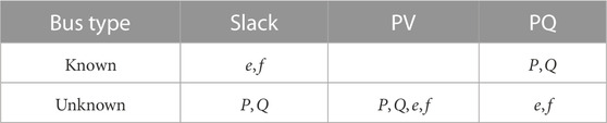
TABLE 1. Bus type classification of PG.

TABLE 2

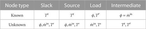
TABLE 2. Node type classification of HN.

The assumptions in Tables 1, 2 are slightly different from the assumptions in Liu et al. (2016), Qin et al. (2019), because, as stated in Section 2, we consider the bi-directional of PG and HN here. Since we consider the CHP type of coupling unit, the ϕ of Source node depends on the P of Slack bus while the P of PV bus depends on the ϕ of Slack node. As a result, these variables are unknown.

To obtain the variations of unknown variables in Tables 1, 2, we should first perform the steady-state calculation of energy flow using the method in (Liu et al., 2016). Thereafter, we obtain the initial distribution of temperatures in pipelines, i.e. the initial condition of Eq. 1. After these preparations, we can start the quasi-dynamic energy flow computation with the procedure in Figure 1. The simulation scenarios were set by interpolation. This is because disturbances can be interpreted as the variation of a specific parameter. Given a disturbance, the proposed method uses interpolation to obtain the value of the simulation parameter on a specific time node. And the parameters are updated once Δt is updated.

FIGURE 1

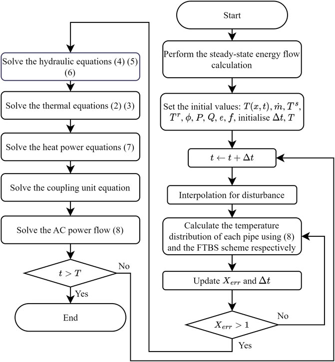
FIGURE 1. Flow chart.

6 Case studies

The proposed method was verified in the following scenarios. All the numerical tests were performed on a laptop equipped with AMD Ryzen 4600 U and 16 GB RAM. The coding language is Matlab R2022a.

6.1 A single pipeline case with measured data

The proposed method was first verified for accuracy in a single-pipeline case. The T^out, $\dot{m}$and other parameter data come from the Luhua CHP plant in Shijiazhuang, Hebei Province, China (Wang et al., 2017). We used the implicit upwind scheme, central scheme, and three kinds of flux limiter schemes to solve Eq. 1 with Δt =180 s, Δx =370 m. The results were compared in Figure 2.

FIGURE 2

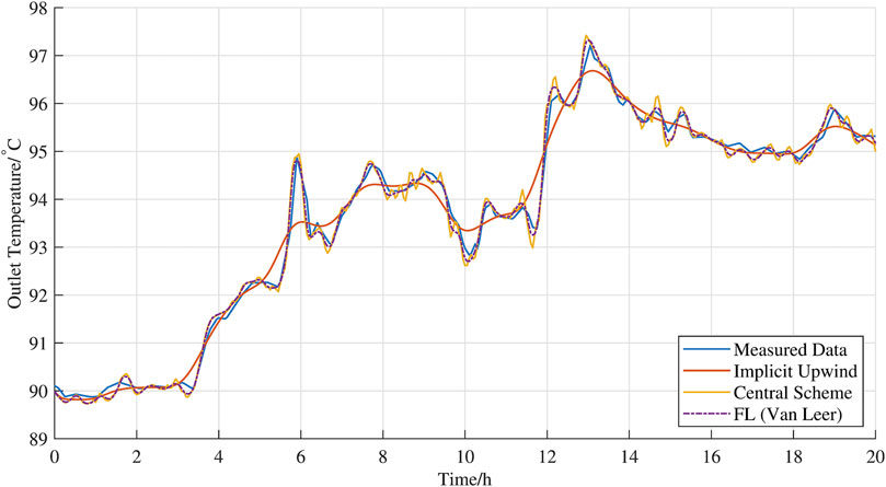
FIGURE 2. Pipeline outlet temperatures.

The root mean squares (RMSEs) of the three schemes, compared with the measured outlet temperatures, were computed in Table 3. The FL schemes have smaller RMSEs than the implicit upwind and central schemes. Among the three kinds of flux limiters, the Van Leer flux limiter has the best accuracy performance, but the C-O and Superbee limiters were all more precise than implicit upwind and central schemes.

TABLE 3

TABLE 3. Computation errors.

6.2 A small system

Next, the proposed method was tested on a small MES to verify its numerical performance in accuracy and efficiency. The system, which comes from (Liu et al., 2016), consists of five heating nodes and four electrical buses. The system is pictorially shown in Figure 3.

FIGURE 3

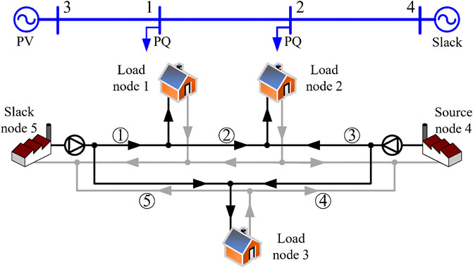
FIGURE 3. Schematic diagram of the small system.

The following methods were performed in the system:

Method 1: The method proposed in (Qin et al., 2019) with implicit upwind scheme.

Method 2: The method proposed in (Yao et al., 2021) with the implicit upwind scheme in Method 1 replaced by the central scheme.

Method 3: The proposed method with fixed Δt.

Method 4: The proposed method with adaptive Δt.

Method 1-Method 3 were performed with Δt =60 s, Δx =10 m. The benchmark trajectories were generated by the MATLAB ODE45 solver with Δt =3 s, Δx =2 m. The benchmark method is explained as follows. First, the spatial derivative in Eq. 1 is discretized with backward difference. Then the PDE becomes a set of ODEs. To further incorporate the nonlinear algebraic equations, the solving schemes are altered as

$\begin{array}{cc}\hfill & \left\{\begin{array}{c}{k}_i=f\left(x_0+\mathrm{\Delta }t{\sum }_{j=1}^{i-1}{a}_{i,j}{k}_j,y_{i-1}\right)\hfill \\ 0=g\left(x_0+\mathrm{\Delta }t{\sum }_{j=1}^{i-1}{a}_{i,j}{k}_j,y_{i-1}\right)\hfill \end{array}\right.i=\mathrm{1,2},\dots ,s-1\hfill \\ \hfill & \left\{\begin{array}{c}{x}_1=x_0+{\sum }_{j=1}^s{b}_j{k}_j\hfill \\ 0=g\left(x_1,y_1\right)\hfill \end{array}\right.\hfill \end{array}$

where x denotes the state variables, that is, the pipe temperatures; y denotes the algebraic variables, that is, the mass flow, power, voltage, etc. s denotes the stage of Runge-Kutta formulae. Here, s = 7. a_i,j, b_j denotes computation parameters. f and g are respectively the ODEs and AEs. The subscript 0 denotes initial/given values while subscript 1 denotes the unknown values. The computation consists of seven stages. In each of the first six stages, we first solve equation $0=g(x_0+\mathrm{\Delta }t{\sum }_{j=1}^{i-1}{a}_{i,j}{k}_j,y_{i-1})$ for y_i−1 and then solve equation $k_i=f(x_0+\mathrm{\Delta }t{\sum }_{j=1}^{i-1}{a}_{i,j}{k}_j,y_{i-1})$ for k_i. Afterwards, we solve for x₁ with $x_1=x_0+{\sum }_{j=1}^s{b}_j{k}_j$, then y₁ with 0 = g (x₁, y₁). The benchmark method has fifth-order temporal accuracy and first-order spatial accuracy. Therefore, using tiny spatial/temporal step sizes, the benchmark can produce enough accurate simulation results.

The total simulation time was set to be 24 h. The supply temperature of node 4 and 5 increased from 100°C to 101°C within 10 min. The simulation results were illustrated in Figures 4, 5. Apparently, the high frequency components in results by Method 1 decayed, which ruined both the supply temperatures and the mass flow rates. And there are obvious fake oscillations in results by Method 2. In contrast, results by Method 3 and Method 4 got rid of high-frequency decaying and fake numerical oscillations and produced precise trajectories. The accuracy improvement was further reflected in Table 4. The root mean square errors of Method 1 to Method 3 were computed against the benchmark. It seems that, due to its TVD property, the proposed method demonstrated the highest accuracy.

FIGURE 4

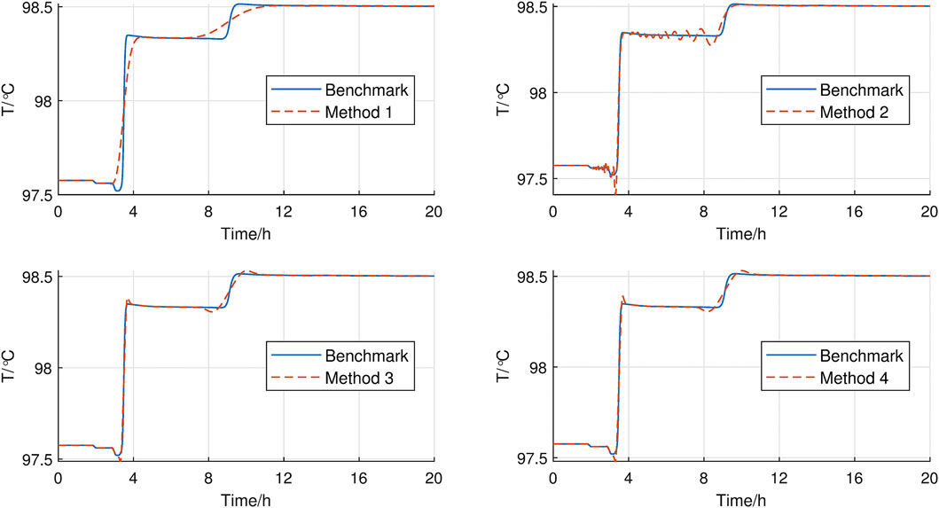
FIGURE 4. Node 2 temperature.

FIGURE 5

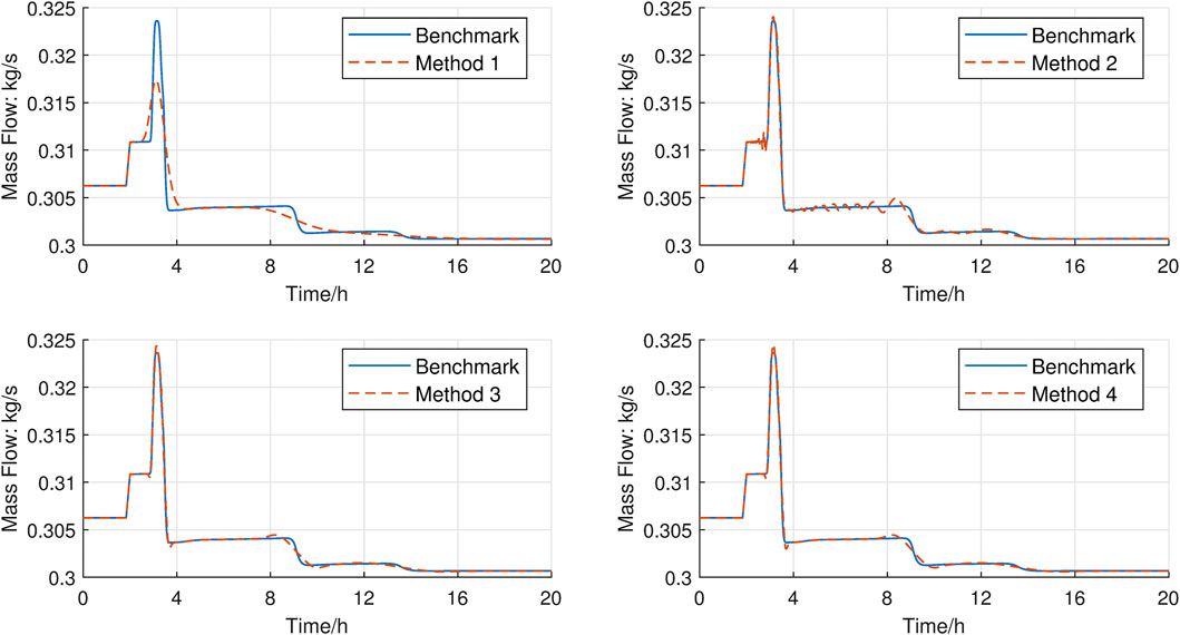
FIGURE 5. Pipe 2 mass flow rate.

TABLE 4

TABLE 4. Computation errors in small-system case.

The total computation times of Method 1-Method 4 were recorded in Table 5. Method 1 and Method 2 had similar computational performance, while Method 3 was more efficient than Method 1 and Method 2. The reasons are as follows. To compute the unknown temperature $T_k^{(n+1)}(2\le k\le M)$ in pipelines, Method 1 and Method 2 would use $T_1^{(n+1)}$, which denotes the temperature of the node that the inlet of the pipeline connects to, and this temperature is unknown. As a result, to obtain $T_k^{(n+1)}$, we should alternatively solve Eq. 1, the hydraulic equations and the thermal equations. While for Method 3 and Method 4, $T_k^{(n+1)}(2\le k\le M)$ do not depend on $T_1^{(n+1)}$ as shown by Eq. 9. Hence, $T_k^{(n+1)}$ can be obtained independently by Eq. 9 and we should only solve the hydraulic equations and the thermal equations together, which decreases the dimensions of the problem. Moreover, the expedite technique further accelerates the overall simulation effectively. Owing to these, the proposed method displayed obviously higher efficiency in this scenario.

TABLE 5

TABLE 5. Total computation time in the small system.

6.3 The Barry Island case

Finally, the proposed method was tested on the well-known Barry Island system. Shown in Figure 6 is the 35-node-9-bus system. Four typical kinds of load trajectories were considered (Qin et al., 2021), and the loads of all nodes changed accordingly. The simulations were performed with the above Method 1-Method 4 with Δt =20 s, Δx =20 m.

FIGURE 6

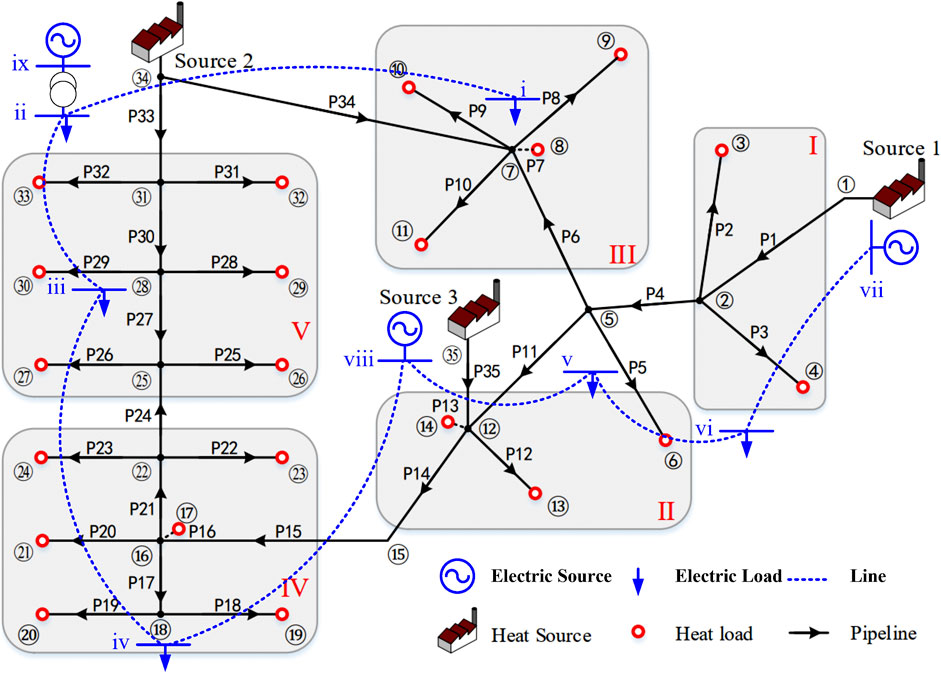
FIGURE 6. Schematic diagram of the Barry Island system.

The simulation results were shown in Figure 7. Like the previous case study, the proposed method depicted the temperature variations more precisely. However, in this case, the computation errors of temperatures have smaller impact on the accuracy of other variables. All the methods produced fairly accurate trajectories of active power. The RMSEs were computed in Table 6. The errors of Method 1 were still bigger than Method 2 and Method 3, but the accuracy of Method 2 was very close to Method 3 in this case.

FIGURE 7

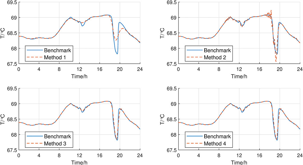
FIGURE 7. Node 10 temperature.

TABLE 6

TABLE 6. Computation errors in barry-island case.

The total simulation computation times were listed in Table 7. As the scale of the system increases, the proposed method still demonstrated obvious efficiency superiority. The expedite technique effectively cut down the total number of simulation time windows and saved nearly fifty percent total computation times.

TABLE 7

TABLE 7. Total computation time in the Barry Island system.

7 Conclusion

Quasi-dynamic EFC in MESs faces the challenges of numerical instability and inefficiency. In view of this, we propose an accurate and efficient solution method for quasi-dynamic EFC in MESs. Firstly, we utilize a scheme with TVD property to discretize the PDE governing thermal dynamics. Thus, the fake oscillation and damping are decreased in an effective way. Secondly, we use two schemes with different accuracy to construct the local truncation error approximation, which helps control the step sizes adaptively. Case studies show that the proposed method was able to accurately depict the thermal dynamics while increased the overall simulation efficiency saliently.

Data availability statement

The original contributions presented in the study are included in the article/Supplementary material, further inquiries can be directed to the corresponding author.

Author contributions

Conceptualization, methodology, software, and writing by YL; part of software, validation, and formatting by KY. All authors contributed to the article and approved the submitted version.

Conflict of interest

The authors declare that the research was conducted in the absence of any commercial or financial relationships that could be construed as a potential conflict of interest.

Publisher’s note

All claims expressed in this article are solely those of the authors and do not necessarily represent those of their affiliated organizations, or those of the publisher, the editors and the reviewers. Any product that may be evaluated in this article, or claim that may be made by its manufacturer, is not guaranteed or endorsed by the publisher.

References

Chen, Y., Guo, Q., Sun, H., Li, Z., Pan, Z., and Wu, W. (2019). A water mass method and its application to integrated heat and electricity dispatch considering thermal inertias. Energy181, 840–852. doi:10.1016/j.energy.2019.05.190

CrossRef Full Text | Google Scholar

Chen, Y., Guo, Q., Sun, H., and Pan, Z. (2021). Integrated heat and electricity dispatch for district heating networks with constant mass flow: A generalized phasor method. IEEE Trans. Power Syst. 36, 426–437. doi:10.1109/tpwrs.2020.3008345

CrossRef Full Text | Google Scholar

Hairer, E., Nørsett, S. P., and Wanner, G. (1993). Solving ordinary differential equations I. second edn. Berlin, Heidelberg, Germany: Springer-Verlag.

Google Scholar

Huang, Y., Sun, Q., Li, Y., Sun, C., and Chen, Z. (2023). Damping technique empowered robust energy flow calculation for integrated energy systems. Appl. Energy 343, 121168. doi:10.1016/j.apenergy.2023.121168

CrossRef Full Text | Google Scholar

Jiang, Y., Wan, C., Botterud, A., Song, Y., and Shahidehpour, M. (2021). Convex relaxation of combined heat and power dispatch. IEEE Trans. Power Syst. 36, 1442–1458. doi:10.1109/TPWRS.2020.3025070

CrossRef Full Text | Google Scholar

Li, Z., Wu, L., Xu, Y., Moazeni, S., and Tang, Z. (2022). Multi-stage real-time operation of a multi-energy microgrid with electrical and thermal energy storage assets: A data-driven MPC-ADP approach. IEEE Trans. Smart Grid 13, 213–226. doi:10.1109/tsg.2021.3119972

CrossRef Full Text | Google Scholar

Li, Z., Wu, L., and Xu, Y. (2021). Risk-Averse coordinated operation of a multi-energy microgrid considering voltage/var control and thermal flow: An adaptive stochastic approach. IEEE Trans. Smart Grid 12, 3914–3927. doi:10.1109/tsg.2021.3080312

CrossRef Full Text | Google Scholar

Li, Z., Wu, L., Xu, Y., Wang, L., and Yang, N. (2023). Distributed tri-layer risk-averse stochastic game approach for energy trading among multi-energy microgrids. Applied Energy 331, 120282. doi:10.1016/j.apenergy.2022.120282

CrossRef Full Text | Google Scholar

Li, Z., Wu, W., Shahidehpour, M., Wang, J., and Zhang, B. (2016). Combined heat and power dispatch considering pipeline energy storage of district heating network. IEEE Trans. Sustain. Energy 7, 12–22. doi:10.1109/tste.2015.2467383

CrossRef Full Text | Google Scholar

Liu, X., Wu, J., Jenkins, N., and Bagdanavicius, A. (2016). Combined analysis of electricity and heat networks. Appl. Energy 162, 1238–1250. doi:10.1016/j.apenergy.2015.01.102

CrossRef Full Text | Google Scholar

Lu, S., Gu, W., Meng, K., Yao, S., Liu, B., and Dong, Z. Y. (2020). Thermal inertial aggregation model for integrated energy systems. IEEE Trans. Power Syst. 35, 2374–2387. doi:10.1109/tpwrs.2019.2951719

CrossRef Full Text | Google Scholar

Ma, R., Liu, H., Geng, J., Zhu, D., Yan, Z., Luo, Z., et al. (2021). Fast decomposed method for dynamic energy flow calculation in integrated electricity and heat system. IEEE Access, 9, 168760–168766. doi:10.1109/ACCESS.2021.3116810

CrossRef Full Text | Google Scholar

Pan, Z., Guo, Q., and Sun, H. (2016). Interactions of district electricity and heating systems considering time-scale characteristics based on quasi-steady multi-energy flow. Applied Energy 167, 230–243. doi:10.1016/j.apenergy.2015.10.095

CrossRef Full Text | Google Scholar

Qin, X., Shen, X., Guo, Y., Pan, Z., Guo, Q., and Sun, H. (2021). Combined electric and heat system testbeds for power flow analysis and economic dispatch. CSEE J. Power Energy Syst. 7, 34–44. doi:10.17775/CSEEJPES.2020.02810

CrossRef Full Text | Google Scholar

Qin, X., Sun, H., Shen, X., Guo, Y., Guo, Q., and Xia, T. (2019). A generalized quasi-dynamic model for electric-heat coupling integrated energy system with distributed energy resources. Appl. Energy 251, 113270. doi:10.1016/j.apenergy.2019.05.073

CrossRef Full Text | Google Scholar

Shen, F., Ju, P., Shahidehpour, M., Li, Z., Wang, C., and Shi, X. (2020). Singular perturbation for the dynamic modeling of integrated energy systems. IEEE Trans. Power Syst. 35, 1718–1728. doi:10.1109/tpwrs.2019.2953672

CrossRef Full Text | Google Scholar

Thomas, J. (1995). Numerical partial differential equations: Finite difference methods. New York, NY, USA: Springer-Verlag.

Google Scholar

Wang, L., Zheng, J., Li, Z., Jing, Z., and Wu, Q. (2022). Order reduction method for high-order dynamic analysis of heterogeneous integrated energy systems. Appl. Energy 308, 118265. doi:10.1016/j.apenergy.2021.118265

CrossRef Full Text | Google Scholar

Wang, Y., You, S., Zhang, H., Zheng, X., Zheng, W., Miao, Q., et al. (2017). Thermal transient prediction of district heating pipeline: Optimal selection of the time and spatial steps for fast and accurate calculation. Appl. Energy 206, 900–910. doi:10.1016/j.apenergy.2017.08.061

CrossRef Full Text | Google Scholar

Yang, J., Zhang, N., Botterud, A., and Kang, C. (2020). On an equivalent representation of the dynamics in district heating networks for combined electricity-heat operation. IEEE Trans. Power Syst. 35, 560–570. doi:10.1109/TPWRS.2019.2935748

CrossRef Full Text | Google Scholar

Yao, S., Gu, W., Lu, S., Zhou, S., Wu, Z., Pan, G., et al. (2021). Dynamic optimal energy flow in the heat and electricity integrated energy system. IEEE Trans. Sustain. Energy 12, 179–190. doi:10.1109/tste.2020.2988682

CrossRef Full Text | Google Scholar

Yao, S., Gu, W., Wu, J., Lu, H., Zhang, S., Zhou, Y., et al. (2022). Dynamic energy flow analysis of the heat-electricity integrated energy systems with a novel decomposition-iteration algorithm. Appl. Energy 322, 119492. doi:10.1016/j.apenergy.2022.119492

CrossRef Full Text | Google Scholar

Yu, R., Gu, W., Lu, H., Yao, S., and Zhang, S. (2022). “Non-iterative calculation of quasi-dynamic energy flow in the heat and electricity integrated energy systems,” in IEEE transactions on power systems. doi:10.1109/TPWRS.2022.3210167

CrossRef Full Text | Google Scholar

Zhang, M., Wu, Q., Wen, J., Lin, Z., Fang, F., and Chen, Q. (2021a). Optimal operation of integrated electricity and heat system: A review of modeling and solution methods. Renew. Sust. Energ. Rev. 135, 110098. doi:10.1016/j.rser.2020.110098

CrossRef Full Text | Google Scholar

Zhang, S., Gu, W., Lu, H., Qiu, H., Lu, S., Wang, D., et al. (2021c). Superposition-principle based decoupling method for energy flow calculation in district heating networks. Appl. Energy 295, 117032. doi:10.1016/j.apenergy.2021.117032

CrossRef Full Text | Google Scholar

Zhang, S., Gu, W., Yao, S., Lu, S., Zhou, S., and Wu, Z. (2021b). Partitional decoupling method for fast calculation of energy flow in a large-scale heat and electricity integrated energy system. IEEE Trans. Sustain. Energy12, 501–513. doi:10.1109/tste.2020.3008189

CrossRef Full Text | Google Scholar

Zhang, S., Gu, W., Zhang, X. P., Lu, H., Lu, S., Yu, R., et al. (2022). Fully analytical model of heating networks for integrated energy systems. Appl. Energy 327, 120081. doi:10.1016/j.apenergy.2022.120081

CrossRef Full Text | Google Scholar

Zheng, W., Zhu, J., and Luo, Q. (2022). Distributed dispatch of integrated electricity-heat systems with 329 variable mass flow. IEEE Trans. Smart Grid, 1. doi:10.1109/TSG.2022.3210014

CrossRef Full Text | Google Scholar

Nomenclature