Integrated energy system planning for a heavy equipment manufacturing industrial park

This paper intends to provide key insights to the manufacturing industrial park designers for selecting the typical days of electric load and planning the resources for energy-producing infrastructure. First, a hybrid time-series model of energy-consuming equipment based on the autoregressive integral moving average model (ARIMA) and temporal convolutional network (TCN) is generated. According to this model, the energy consumption (EC) curve of large equipment in the industrial park can be depicted. Moreover, the present study designed a TLSM-IPML (typical load stratification method for industrial parks with manufacturing load) algorithm based on the typical day-selected method. The data clustering method is utilized to analyze the energy usage characteristics. Furthermore, an energy usage-based planning model is proposed, network constraints are considered, and a multi-optional method is designed to solve the problem. Finally, case studies validate the superior performance of TLSM-IPML in analyzing the characteristics of energy consumption and planning the model in reducing MES (manufacturing industrial factory integrated energy system) economic costs.

1 Introduction

With the evolution of energy infrastructure, integrated energy systems (IES) have been developed to improve efficiency and lower carbon emissions. The electrical systems in industrial parks, especially heavy equipment manufacturing, face challenges due to variable energy consumption, high peak loads, and operational schedules (Shao et al., 2023; Lv et al., 2020). Maintaining power quality is critical to prevent disruptions, but the long-term effects on equipment and efficiency are underexplored (Araghian et al., 2023; Zhong et al., 2018). Integrating renewable energy is essential for reducing emissions, yet the economic feasibility and optimization of large-scale integration need more study (Mehrjerdi et al., 2021). Energy storage solutions like batteries are vital for mitigating peak loads and improving system efficiency, but their integration requires further research (Pombo et al., 2023). The evolution of energy infrastructure has led to integrated energy systems (IES) that improve efficiency and lower carbon emissions by supplying heat and electricity simultaneously using the combined cold, heat, and power (CCHP) approach. However, effectively modeling large-scale equipment in industrial parks remains challenging. To address this, a template-based load modeling technique is developed for a better representation of industrial energy consumption within an IES. Overall, advanced strategies are needed to predict and manage energy fluctuations, optimize load distribution, maintain power quality, integrate renewable energy, and enhance storage solutions, addressing gaps in current research and practice.

To gain insights into users’ electricity consumption behaviors, data clustering algorithms are utilized to analyze load data. Density-based clustering algorithms like DBSCAN (Fang et al., 2023) are popular for identifying dense regions and measuring point density. Despite its effectiveness (Fan et al., 2019), DBSCAN’s performance is highly sensitive to parameters like neighborhood radius and minimum points. OPTICS (Mahran and Mahar, 2008) extends DBSCAN to handle varying densities but has a high computational cost. DPeak and its variants (Muja and Lowe, 2014; Cheng et al., 2021) identify density peaks for non-convex clusters but require complex parameter tuning. The mean shift (Fan et al., 2017) shifts points toward higher densities, converging at local maxima without predefined cluster numbers, but struggles with high-dimensional data due to computational expense. DCore (Chen et al., 2018) improves core point identification but involves intricate parameter settings. These methods face challenges such as parameter sensitivity and computational complexity, limiting their effectiveness on large-scale data. For instance, K-means has a complexity of $O(ktn)$, and DBSCAN runs in $O(n^2)$. Due to these high complexities, most clustering approaches struggle with large-scale data.

Recent studies have constructed renewable energy models for new-energy park planning, but handling the complexity of grid connections for renewable energy is challenging. Non-linearity and modeling complexity often lead to overlooked constraints in the internal energy network and operational uncertainties. Martinez Cesena and Mancarella (2019) proposed a robust operational optimization framework for smart districts with multi-energy devices and integrated energy networks (Rhodes et al., 2014). Building on this, Good and Mancarella (2019) considered network constraints for IES planning yet faced challenges in engineering applications due to neglecting the non-linearity of hub equipment. Clegg and Mancarella (2016) addressed these difficulties by introducing a unified energy flow model with refined device models. Despite demonstrating the coupling model of integrated energy systems (IES), the increased system scale complicates computation and convergence. To address this, Zhao et al. (2021) developed a decomposed method for the IES under grid-connected modes, and Zhang et al. (2021) extended this to combine heat, gas, and electric systems for better computational performance. Improving hydrogen production efficiency via electrolysis is also a key focus, with studies like Fu et al. (2020) and Li et al. (2019) exploring the impact of electrolyzer sizes, system efficiencies, and optimal dispatch models. However, these studies often face issues such as ignoring the temporal dynamics of equipment energy use, failing to select typical load days effectively, and lacking a comprehensive analysis of operation and maintenance costs. These gaps highlight the need for efficient and scalable solutions in integrated energy management.

In distribution system planning, the total cost depends on the efficient use of renewable distributed generation, related to network capacity and system loading levels. Demand controllability and connections with renewable generation also impact optimal energy infrastructure distribution. However, existing studies often overlook the temporal dynamics of large equipment energy use, which is critical for accurate energy planning and optimization. This paper proposes a novel time-series energy consumption (EC) model and uses clustering methods to select typical days for load analysis, better analyzing the EC and load characteristics of manufacturing industrial parks. Additionally, the operation and maintenance costs of large-scale energy-consuming equipment and their benefits are considered, emphasizing their role in the park’s overall objective function. The existing literature falls short in the following ways: 1) it ignores equipment temporal dynamics, 2) fails to effectively select typical load days, and 3) lacks a comprehensive analysis of operation and maintenance costs. The main contributions of this paper are as follows:

• First, a hybrid time-series model of energy-consuming equipment based on the autoregressive integral moving average model (ARIMA) and temporal convolutional network (TCN) is generated. According to this model, the EC curve of large equipment in the industrial park can be depicted.

• Second, in this paper, a load clustering method based on the TLSM-IPML algorithm is proposed for selecting typical days of electrical loads in manufacturing industrial parks. The impact of energy use behavior on the planning results is revealed.

• Third, a maintenance model is proposed to analyze the adaptive maintenance of energy-consuming equipment. Moreover, this paper suggests a manufacturing industrial integrated energy system (MES) planning model considering the load characteristics to minimize the total cost, including investment in facilities, operation, purchase energy costs, and benefits from energy production.

The rest of this paper is as follows: The industrial park’s renewable energy models and large types of equipment are introduced in Section 2. The load clustering method based on the TLSM-IPML algorithm is introduced, and the clustering efficiency of different clustering methods is comparatively analyzed in Section 3. The objective and restriction functions are proposed in Section 4. Section 5 shows the solution method of the planning model. In addition, the case studies are given in Section 6. Last, conclusions are drawn in Section 7.

2 Representation of system generation and energy-consuming equipment

This section introduces the MES model with nonlinear power and gas flow equations, including the resource endowment assessment, renewable energy equipment models, and ESS model. Furthermore, a mathematical model of EC equipment is built to conduct EC analysis.

2.1 Energy-supplying equipment

In this section, models of the energy equipment are shown. The structure of the IES contains the following parts: the photovoltaic power generation model, wind power generation model, and HP model.

2.1.1 Photovoltaic power generation model

Solar energy is a clean and abundant resource. Estimating solar energy resources involves evaluating total solar radiation. This parameter is compared with standard data to determine solar energy levels, as shown in Table 1, Total solar radiation is the sum of direct and scattered radiation.

Table 1

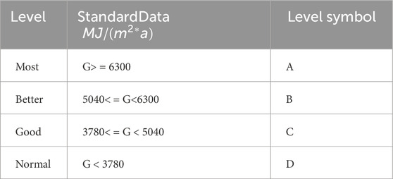
Table 1. Annual total solar radiation level.

After understanding the level of solar energy resources, photovoltaic power generation equipment will be deployed. The output power of photovoltaic power generation equipment is mainly related to the light intensity, operating conditions, and ambient temperature received by the photovoltaic array. The relationship between radiation intensity and the output power of a PV module is described by a linear function.

2.1.2 Wind turbine

To plan a new energy park, the wind energy potential of the location must be assessed before design. The two-parameter Weibull distribution is widely used for analyzing wind speed. Wind energy potential is typically assessed using wind velocity and wind power density data (Chauhan and Saini, 2014). $\bar{V}$ is the mean wind speed; ${\bar{W}}_e$ is the average effective wind energy density.

After the data of ${\bar{W}}_e$ and $\bar{V}$ at a certain height have been known, the level of the wind energy resources can be obtained by comparing them with the standard data in Table 2. If the wind energy resources are the first level, it is not suggested to connect the wind power to the grid. The result of the comparison of the two kinds of data can show whether it is suitable or not to connect wind power to the grid.

Table 2

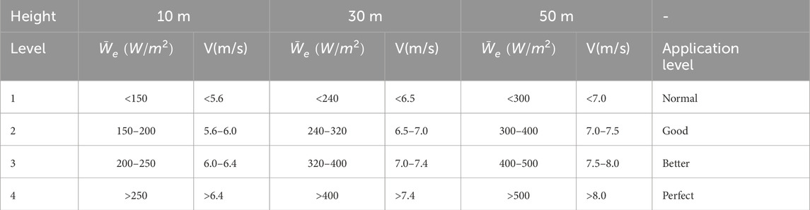
Table 2. Wind energy resource level.

The wind speed mainly determines the output power of the wind turbine generator. Figure 1 shows the wind speed power function of the wind turbine generator. When $v<v_{in}$, the wind turbine has no output. When $v>v_{in}$, the turbine starts working, and its output power increases nonlinearly with wind speed; $v_{in}$ is the cut-in wind speed. When $v_N\le v\le v_{\mathit{out}}$, the turbine maintains a constant rated output power, $P_{WT,N}$, and $v_N$ is the rated wind speed. When $v>v_{\mathit{out}}$, the turbine shuts down for safety, which is the cutout wind speed.

Figure 1

Figure 1. Wind speed–power diagram.

2.1.3 CCHP turbine

Combined cooling, heating, and power (CCHP) systems generate electricity, heat, and cooling from one source, such as natural gas. A prime mover (e.g., gas turbine) produces electrical power (1 MW–10 MW). Waste heat is recovered (600–800$°$C) for heating or driving absorption chillers. This increases efficiency (up to 80$\%$), reduces fuel use, and lowers emissions, making CCHP suitable for industrial parks and hospitals.

2.1.4 Waste heat recovery system

A waste heat turbine is a waste heat collection device that collects waste heat from the heat pump and CCHP and turns waste heat into high-temperature gas, which can be used in steam turbines for power generation. The physical model of the waste heat recovery system is as follows: the main function of a waste heat boiler is to use waste heat to generate steam. The power generation capacity of the waste heat recovery system is calculated as follows Equation 1:

$P_{wr}=Q_{wr,in}{\eta }_{wr},(1)$

where $Qwr,in$ is the flue gas thermal power absorbed by the system, kW; ${\eta }_{wr}$ is the efficiency of the waste heat recovery system; and $P_{wr}$ is system power generation, kW. The process of flue gas recovery is shown in Figure 2. The boiler burns gas or coal, producing flue gas. Before discharge, the flue gas undergoes treatments like desulfurization and denitrification. Waste heat from the flue gas can be recovered by passing it into a waste heat boiler, which generates steam without additional fuel. This steam is then sent to a steam turbine.

Figure 2

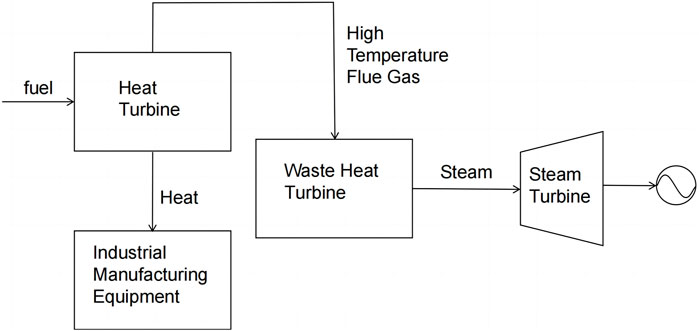
Figure 2. Waste heat recovery process.

2.1.5 Hydrogen production system

Hydrogen is produced using an electrolyzer system which converts electrical energy into chemical energy using water electrolysis technology. The amount of hydrogen produced from the electrolyzer is directly proportional to the current supplied to the electrolyzer system (Zeng et al., 2014).

The electrolyzer conversion efficiency behavior is crucial for the economic and technical analysis of hydrogen production. By improving the electrolyzer efficiency, the hydrogen production cost can be minimized. The conversion efficiency of the electrolyzer system represents the ratio of the output energy content of the produced hydrogen at the electrolyzer stack to the input DC power energy into the electrolyzer stack (Yodwong et al., 2020).

2.2 Energy storage equipment

Batteries are often used to store surplus PV power and grid power during low grid electricity prices, to be used later when demand exceeds PV power generation and during times of high grid electricity prices. They are already a very mature energy storage technology. The thermal storage tank can store excess heat in it. When there is a heat load demand, the heat in the thermal storage tank can be used for heating, maximizing the energy efficiency of the entire system. For the electricity and heat storage equipment of the integrated energy system, a general model can be used to represent the process of energy accumulation and release, as shown in following Equations 2−6:

$E_x^{t+1}=E_x^t\left(1-{\delta }_x\right)+\left(X_{ch,x}^t{\eta }_{ch,x}-\frac{X_{\mathit{dis,x}}^t}{{\eta }_{\mathit{dis,x}}}\right)\mathrm{\Delta }t,(2)$

$0⩽X_{\mathit{chp,x}}^t⩽u_x^t\cdot {\rho }_{ch,x}^{\mathit{max}}{E}_x^P,(3)$

$0⩽X_{\mathit{dis,x}}^t⩽\left(1-u_x^t\right)\cdot {\rho }_{\mathit{dis,x}}^{\mathit{max}}{E}_x^P,(4)$

$SO{C}_x^{\mathit{min}}{E}_x^P⩽E_x^t⩽SO{C}_x^{\mathit{max}}{E}_x^P,(5)$

$E_x^{T+1}=E_X^1.(6)$

where X represents the type of energy, including both P for electricity and H for heat; the subscript x is the energy storage equipment; Bat and Tst are electricity and heat storage, respectively; Etx indicates the energy stored by the energy storage device in period t; δx is the energy self-loss rate of the energy storage equipment; ηch,x and ηdis,x are the energy storage efficiency and energy discharge efficiency of the energy storage equipment, respectively; X_t ch,x and X_t dis,x are the energy charge and discharge power, respectively; uxt is the energy storage and discharge identifier of the energy storage equipment, which is a 0-1 variable; when it is 1, it means that the energy storageequipment is storing energy in period t; ρ_max ch,x and ρ_max dis,x are the maximum charging and discharging coefficients of the energy storage device, which represent the proportion of the maximum energy storage and discharging power of the energy storage device to the total capacity of the device; SOC_min x and SOC_maxx are the minimum and maximum energy storage ratios of the energy storage device, respectively; EPx is the planned installation capacity of the energy storage device.

2.3 Energy-consuming equipment

In this section, we build detailed energy consumption models for key equipment within the industrial park. The equipment includes air compressors, coil factory ovens, and charging stations. By simulating the energy usage patterns of these devices, we aim to optimize energy management and improve efficiency, providing a framework for effective energy-saving measures and sustainable industrial operations.

2.3.1 Air compressor

Compressing air consumes electricity directly. To model the energy consumption (EC) of an air compressor, key factors include the type, number, operating efficiency, and start–stop times of the compressors. The mathematical model for an air compressor station with $m$ types and $n_i$ compressors of each type is as follows Equation 7:

$P_{ac}={\displaystyle \sum _{n=1}^m}{\displaystyle \sum _{j=1}^n}\frac{n_{i,j}{P}_i{t}_{i,j}}{{\eta }_i},(7)$

where $m$ represents the number of types of air compressors in the air compressor station; $n$ represents the number of different types of air compressors; $n_i$ is the number of equipment of type i; $P_i$ is the rated power (kW) of type i air compressor; ${\eta }_i$ is the energy efficiency of the ith type air compressor; and $t_{i,j}$ is the operating time h) of the ith type air compressor.

2.3.2 Coil branch factory oven

To establish a mathematical model of an oven, the main goal is to describe and predict the temperature distribution, heating time, and EC within the oven. This model can be used to optimize oven operating conditions, improve energy efficiency, and ensure product quality. For unsteady one-dimensional heat conduction, the equation is, as shown in Equation 8:

$P_{OF}={\displaystyle \sum _{i=1}^n}{P}_i{t}_i+m{c}_p\left(T_t-T_i\right)+\xi S\left(T_i-T_{\mathit{aim}}\right)t,(8)$

where $P_i$ is the rated power of the oven (kW); $t_i$ is the operating time of the first oven h); $m$ is the equivalent mass of the object to be burned in the oven (kg); $c_p$ is the specific heat capacity of the object to be burned $(J/(kg\cdot ◦C))$; $T_t$ is the target temperature; $T_1$ is the initial temperature; $T_{\mathit{aim}}$ is the ambient temperature; $\xi$ is the overall heat transfer coefficient of the oven $(W/(m^2\cdot ◦C))$; and $S$ is the surface area of the oven $(m^2)$. The model considers the effects of electrical EC, operating time, temperature, and heat transfer on EC. This model is used to evaluate an oven’s EC more fully and optimize its operating conditions to increase energy efficiency.

2.3.3 Charging pile

The efficiency of charging piles is affected by many factors, including charging current, voltage stability, impedance of charging lines, and quality of charging equipment. Charging piles will produce certain losses during the charging process, affecting their energy efficiency, including losses during the power conversion process and losses caused by line resistance. Based on the above analysis, the charging pile model is built as follows Equation 9:

$P_{cp}=P_{cp,cap}\frac{1}{{\eta }_{cp}}M,(9)$

where $P_{cp,cap}$ is the rated power of the charging pile (kW), ${\eta }_{cp}$ is the energy efficiency of the charging pile (percent, $\%$), that is, the ratio of actual output energy to input energy; and $M$ is the charging mode of the charging pile, such as fast charging and slow charging.

2.3.4 Construction of the sequential model for large-scale energy-consuming equipment

To analyze the impact of random large-scale energy consumption (EC) in heavy equipment manufacturing industrial parks, the EC and time dependence of energy-consuming equipment should be modeled accurately. This section proposes a general ARIMA model structure to simulate the EC curve, where $y(1),y(2),y(N)$ is an observational time-series data modeled by a stochastic process $Y(t)$. The standard autoregressive integrated moving average (ARIMA) model of $Y(t)$, denoted as ARIMA$(p,d,q)$, has the following expression as shown in Equation 10:

$P_t={\lambda }_0+{\displaystyle \sum _{i=1}^p}{\varphi }_i{Y}_{t-i}+\left({\epsilon }_t-{\displaystyle \sum _{j=1}^q}{\theta }_j{\epsilon }_{t-j}\right),(10)$

where $Y_t$ and ${\epsilon }_t$ are the actual value and random error of period t, respectively; $p$ is the order and coefficient of the autoregressive (AR) component of ARIMA; ${\varphi }_i$ is the parameter of the autoregressive model, indicating the weight of past observations in the time series; and ${\theta }_j$ is the parameter of the moving average model, which represents the weight of the error of past observations. In addition, the unified model of the EC process of large-scale energy-consuming equipment in heavy equipment manufacturing industrial parks is as follows:

$Y_t=f\left(X_t\right)+{\epsilon }_t,(11)$

where $Y_t$ is the EC at time $t$ and ${\epsilon }_t$ represents the error term, which represents random situations, such as equipment failure.

To forecast seasonal and residual components using ARIMA, it is important to ensure that the time series is stationary as this is necessary for building a useful ARIMA model. Stationary series have constant statistical properties over time. The augmented Dickey–Fuller (ADF) test can be used to check for stationarity. If the series is non-stationary, differencing operations should be applied. The process is shown as following Equation 12.

${\nabla }^d{Y}_t={\nabla }^{d-1}{Y}_t-{\nabla }^{d-1}{Y}_{t-k},(12)$

where $d$ is the number of times the seasonal or residual components differ and $k$ is the time step of the difference operation. TCN is a special one-dimensional CNN composed of causal convolution, dilated convolution, and residual block. It processes input sequences directly, learning local features effectively. Unlike traditional RNNs like LSTM and GRU, TCN uses causal and dilated convolutions along with residual connections to learn sequence features recursively. Causal convolution ensures that the value at time $t$ only depends on values at $t$ and earlier times. For a one-dimensional input $l\in R^T$ and a filter $f:0,\dots ,k-1$, an ordinary one-dimensional causal convolution layer is defined as follows Equations 13, 14:

$F\left(l_t\right)=\left(l*f\right)\left(t\right)={\displaystyle \sum _{j=0}^K}{f}_j{l}_{t-j},(13)$

$\widetilde{seq}=\left(F\left(l_1\right),F\left(l_2\right),\dots F\left(l_T\right)\right),(14)$

where $\widetilde{seq}$ is an output sequence, $K$ is the convolution kernel size, and $F(\cdot )$ is a convolution calculation.

After the TCN model is built, it can be applied to the EC modeling of large-scale electrical equipment in a heavy equipment manufacturing industrial park. The TCN model combines traditional time-series analysis and deep learning for forecasting. First, the ARIMA model captures the linear trend and periodicity in the data to obtain the basic trend EC. Then, the residuals from the ARIMA model are used as the input for the TCN model to capture nonlinear patterns and long-term dependencies. At this time, the residuals are calculated as $\widehat{{\epsilon }_t}=TCN({\epsilon }_{t-1},{\epsilon }_{t-2},\dots ,{\epsilon }_{t-k})$.

The TCN model uses a self-attention mechanism to effectively capture relevant information in sequence data, improving the accuracy and robustness of EC modeling for large-scale equipment in heavy equipment manufacturing industrial parks. The flowchart of the hybrid ARIMA and TCN model is shown in Figure 3.

Figure 3

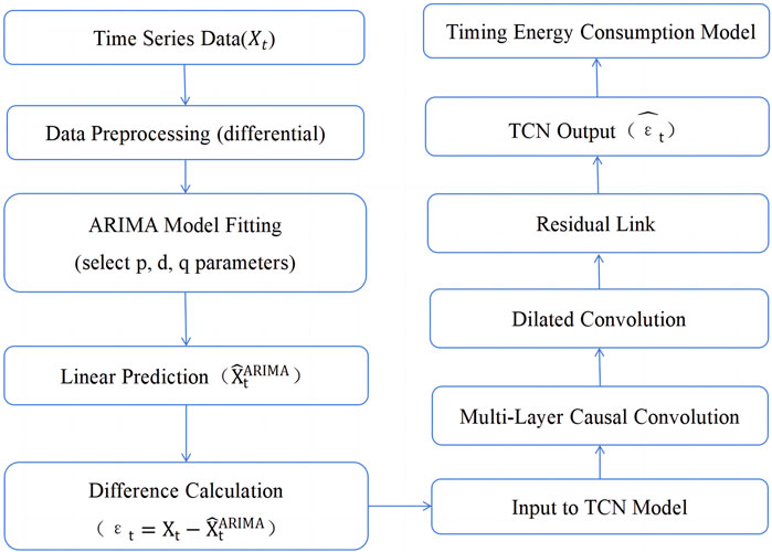
Figure 3. Flow chart of the hybrid timing model based on ARIMA and TCN.

Figure 4

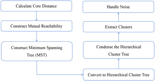
Figure 4. TLSM-IPML clustering process.

Based on the above energy usage patterns of large equipment manufacturing industrial parks, an overall model is built for the energy usage patterns of large equipment in heavy equipment manufacturing industrial parks. Due to equipment wear and energy loss in the production process, the total system EC at time $t$ $(P_{i,equ}^t)$ is divided into four parts: transmission EC $(P_{\mathit{tra}}^t)$, conversion EC $(P_{\mathit{con}}^t)$, standby EC $(P_{\mathit{sta}}^t)$ and peak load, and regulation EC $(P_{\mathit{par}}^t)$. This classification method is based on general criteria for the production EC classification. Thus, the total EC in heavy equipment manufacturing industrial parks can be obtained as follows Equation 15:

$P_{i,equ}^t=P_{\mathit{tra}}^t+P_{\mathit{con}}^t+P_{\mathit{sta}}^t+P_{\mathit{par}}^t+\widehat{{\epsilon }_t},(15)$

where $P_{\mathit{tra}}^t$ includes losses on power lines and losses during the transport of natural gas, oil, etc. The EC of the transmission and distribution process can be expressed as follows Equation 16:

$P_{\mathit{tra}}^t={\displaystyle \sum _{i=1}^n}\left({\int }_0^{t_{\mathit{tra}}^i}{E}_{\mathit{tra}}^{t}dt\right)+{\displaystyle \sum _{i=1}^m}\left({\int }_0^{t_G^i}{E}_{\mathit{tra}}^{t}dt\right),(16)$

where $n$ is the total number of energy types. $E_{\mathit{tra}}^t$ and $t_{\mathit{tra}}^i$ are the transmission power and time, respectively.

In the energy system, energy is lost when converting one form of energy to another, for example, the conversion of fuel to electricity (such as in combustion power plants) or the conversion of electricity to mechanical energy (such as in electric motors). Thus, $P_{\mathit{con}}^t$ is expressed as follows Equation 17:

$P_{\mathit{con}}^t={\displaystyle \sum _{i=1}^n}\left({\int }_0^{t_{\mathit{gen}}^i}{E}_{\mathit{gen}}^{t}dt\right)+{\displaystyle \sum _{i=1}^m}\left({\int }_0^{t_{\mathit{mot}}^i}{E}_{\mathit{mot}}^{t}dt\right),(17)$

where $n$ is the total number of generators in MES. $m$ is the total number of motors in MES. $E_{\mathit{con}}^t$ and $E_{\mathit{mot}}^t$ are the power during fuel combustion and motor operation, respectively. $t_{\mathit{gen}}^i$ and $t_{\mathit{mot}}^i$ are combustion and operation time, respectively.

In the energy system, equipment consumes energy in the standby mode or during low-efficiency operation, for example, the energy consumption of power generation equipment at low load or idle times or household appliances in the standby mode. Thus, the standby EC is given as follows Equation 18:

$P_{\mathit{sta}}^t={\displaystyle \sum _{i=1}^n}\left({\int }_0^{t_{\mathit{grid}}^i}{E}_{\mathit{grid}}^{t}dt\right)+{\displaystyle \sum _{i=1}^m}\left({\int }_0^{t_{\mathit{set}}^i}{E}_{\mathit{set}}^{t}dt\right),(18)$

where $n$ is the total number of energy-generating infrastructures. $m$ is the total number of generator sets. $E_{\mathit{grid}}^t$ and $E_{\mathit{set}}^t$ are the power during a standby mode of energy-generating infrastructures and generator set and motor operation, respectively. $t_{\mathit{grid}}^i$ and $t_{\mathit{set}}^i$ are standby times of the grid and sets, respectively.

In the energy system, additional energy consumption occurs when adjusting the power output to meet load fluctuations and peak demand, for example, when the power grid starts, backup generators or peaking power plants meet high-demand periods, leading to increased energy consumptions. Thus, the EC of peak load and regulation can be expressed as follows Equation 19:

$P_{\mathit{par}}^t={\displaystyle \sum _{i=1}^n}\left({\int }_0^{t_{\mathit{peak}}^i}{E}_{\mathit{peak}}^{t}dt\right)+{\displaystyle \sum _{i=1}^m}\left({\int }_0^{t_{\mathit{frv}}^i}{E}_{\mathit{frv}}^{t}dt\right),(19)$

where $n$ is the total number of peak load units. $m$ is the total number of frequency and voltage regulation units. $E_{\mathit{peak}}^t$ and $E_{\mathit{frv}}^t$ are the power during the peak shaving frequency and voltage regulation, respectively. $t_{\mathit{peak}}^i$ and $t_{\mathit{frv}}^i$ are the peak shaving frequency and voltage regulation time, respectively.

The proposed model for heavy equipment combines ARIMA and TCN to handle linear and non-linear energy consumption patterns. Regular updates to the TCN and dynamic adjustments to the ARIMA ensure that the model remains accurate and responsive to changes. This approach maintains reliability without a complete overhaul when conditions change, making it suitable for evolving operations.

3 TLSM-IPML clustering method

In the previous section, we developed an energy model for the industrial park. This chapter uses TLSM-IPML clustering to select typical days, capturing time-related and seasonal energy consumption patterns. This helps in understanding usage and applying ARIMA and TCN models accurately, improving energy management and efficiency.

3.1 Basic definition and process of the TLSM-IPML clustering method

In this section, the TLSM-IPML clustering method is introduced. The core idea behind TLSM-IPML is to convert the problem of density-based clustering into a problem of finding the areas of high density in the dataset and then hierarchically clustering these dense areas based on their density and separation. It operates on the principle that clusters are areas of higher density than their surroundings in the data space.

3.1.1 Basic ideas of the TLSM-IPML clustering method

As noted in Zhang et al.’s (2023) study, DBSCAN struggles with large-scale data due to its high complexity. Our analysis shows that points $p$ and $q$ in the dataset should have similar neighborhoods if they are close, meaning a point tends to share its neighbors’ type. TLSM-IPML improves on DBSCAN by automatically selecting suitable neighborhood values for clustering. It introduces the interconnection distance $r{l}_m(p)$ to form stable clusters and reduce noise interference. A minimum spanning tree (MST) is then used for hierarchical clustering. TLSM-IPML adapts to data’s characteristics, making it effective for complex datasets with varying density distributions.

In this article, $n$ represents the number of days in the year for the heavy equipment manufacturing industrial park and $m$ represents the number of hours per day. Therefore, the dataset is the annual electrical load data on the park. Let $X=\left\{X_1,X_2,X_3,\dots ,X_n\right\}$ be a set of $n$ objects, where each object $X_i$ is represented by $x_{i,1},x_{i,2},\dots ,x_{i,m}$. Here, $m$ represents the number of types of data. We use relative density to divide the dataset into low and high-density parts. The relative density of data points is defined as follows Equation 20:

$rd\left(i\right)=\frac{k}{{\sum }_{n=1}^{k}dist\left(x_{i,j}\right),x_{n,j}},(20)$

where $dist(x_{i,j},x_{n,j})$ represents the Euclidean distance between points $x_{i,j}$ and $x_{n,j}$ and $k$ is the number of nearest neighbors of $x_{i,j}$. To identify low-density data points, two parameters are defined: $k$ (number of nearest neighbors) and $t$ (density threshold). $k$ determines the neighbors involved in the relative density calculation, and $t$ sets the threshold for low density. We calculate the relative density $rd(i)$ for each data point $x_{i,j}$ and compare it with $t$. If $rd(i)<t$, the data points are merged into the low-density set $L$, which is expressed as $L=\left\{x_{i,j}|rd(i)<t\right\}$.

Using core distance and interconnection distance as measurements is more appropriate. The core mathematical concepts and formulas of the TLSM-IPML algorithm are given as follows:

Core distance: For a given minimum number of samples $m$ and distance metric $d$, the core distance of a point $p$ is defined as the distance to the $m$-th immediate neighbor point: $c{d}_m(p)=min\left\{r:\left|N(p,r)\right|\ge min{P}_{ts}\right\}$. Among them, $N(p,r)$ represents the neighborhood surrounding point p within radius r, and $\left|N(p,r)\right|$ represents the number of points in this neighborhood. The calculation of core distance determines the potential of each typical day as a cluster center, which is critical for the subsequent construction of minimum-spanning trees and judging whether connections between points should exist.

Interconnect distance: Interconnect distance is defined based on the core distance and is used to evaluate the reachability between two points. For two points $p$ and $q$, their interconnection distance is defined as $i{d}_m(p)=max\left\{c{l}_m(p),c{l}_m(q),D(p,q)\right\}$. The interconnection distance from $p$ to $o$ is at least the core distance and not less than $D(p,o)$. Here, $D(p,q)$ is the D-Euclidean distance between points $p$ and $q$, indicating that the interconnection distance from $p$ to $q$ is at least $p$’s core distance and not less than $D(p,q)$. This helps the algorithm adapt to different density levels in the dataset, allowing for more reasonable connections between points. This directly impacts the construction of the hierarchical clustering tree and the final cluster formation.

Minimum spanning tree (MST): Using core distance and reachability distance, a minimum spanning tree on a point set is constructed, where the weight of each edge is the reachability distance.

A single-chain hierarchical clustering process, based on MST and using reachability distance, is applied. Cluster centers are selected through a stability-based method to calculate the sum of reachable distances for each potential cluster, identify clusters that remain stable until distance increases (indicating decreased density), and select clusters by cutting the longest edges to split the tree. Points not meeting stability or size requirements are considered noise. The steps of the TLSM-IPML algorithm are as follows Figure 4:

1) Initially, the dataset is transformed into a graph represented as a minimum spanning tree (MST) and calculated based on the mutual reachability distance between points. This process ensures that the distances are normalized even in datasets with varying densities to reflect the density landscape more accurately. $d_{\mathit{mreach-k}}(a,b)=max\left\{c{d}_k(a),c{d}_k(b),dis(a,b)\right\}$, where $c{d}_k(a)$ and $c{d}_k(b)$, respectively, represent the core distance defined by the parameters $k$ of point and point, and $dis(a,b)$ is the original metric distance of point $a$ and $b$.

2) Using the MST, TLSM-IPML constructs a hierarchy of clusters by removing the longest edges first and separating the graph into smaller, denser components. This process resembles finding valleys in a topological landscape, where each valley represents a potential cluster.

3) The algorithm then condenses the hierarchy to remove the less significant branches. This step simplifies the cluster hierarchy, making it easier to analyze and interpret.

4) Finally, TLSM-IPML extracts the clusters from the condensed hierarchy based on their stability. A cluster’s stability is a measure of its persistence over the range of distances considered; more stable clusters are considered significant, while less stable ones are treated as noise.

As shown in Algorithm 1, there are two significant parameters: minimum cluster size (MCS) and minimum sample (MS). First, MCS sets the minimum number of points required for a set to be considered a cluster. For electrical load data in manufacturing parks, selecting an appropriate MCS is crucial, impacting the number and size of identified clusters. Larger MCS values yield fewer but larger, more stable clusters, while smaller values detect more smaller clusters. MCS selection can be guided by initial data exploration or domain expert advice, especially when daily load patterns are similar. In addition, MS determines when a point is considered a core point in the algorithm. Higher MS leads to denser core areas, which is beneficial for identifying noisy data. Adjusting MS is necessary based on dataset characteristics to distinguish major trends from random fluctuations or outliers.

Algorithm 1.TLSM-IPML clustering algorithm.

1: Input: dataset $D$, minimum cluster size $min\text{\_}pts$

2: Output: cluster labels for each point in $D$

3: procedure TLSM-IPML($D,min\text{\_}pts$)

4:   compute core distances for all points

5:   compute mutual reachability distances

6:   construct MST from mutual reachability distances

7:   ExtractClusters(MST)

8:   assign cluster labels based on stability

9: procedure

10: procedure ExtractClusters(MST)

11:   initialize cluster hierarchy $H$

12:   while MST is not empty do

13:    remove longest edge $e$ from MST

14:    form two new clusters by splitting at $e$

15:    compute stability of new clusters

16:    update hierarchy $H$ with new clusters

17:   while

18:   return $H$

19: procedure

20: return cluster labels

In short, the TLSM-IPML method is suitable for typical daily cluster analysis of electrical load datasets in manufacturing industrial parks because it can effectively handle changes in data density, noisy data, and complex data structures and does not require pre-specification. The number of clusters and these properties make it ideal for analyzing this data type.

3.2 Cluster validity analysis

When using TLSM-IPML or other clustering algorithms for data analysis, determining the optimality of the clustering effect relies on several mathematical evaluation indicators. To evaluate the effectiveness of clustering, we analyze three key parameters: the Silhouette coefficient, the Davies–Bouldin index, and the Calinski–Harabasz index. These metrics provide a comprehensive view of clustering quality. The following are several commonly used mathematical models and evaluation indicators that can help demonstrate and evaluate the quality of clustering results.

3.2.1 Effectiveness analysis parameters

Evaluating the effectiveness of clustering methods ensures that the clustering results are meaningful and valuable for practical applications. To comprehensively assess the quality of clustering, several metrics are commonly used. The following three key parameters measure the quality of clustering from different perspectives.

• Silhouette coefficient: This metric measures the cohesion and separation of clusters, with higher values indicating better-defined clusters.

• Davies–Bouldin index: This index evaluates the average similarity ratio of each cluster with its most similar cluster, with lower values representing better clustering quality.

• Calinski–Harabasz index: This index assesses the ratio of the sum of between-cluster dispersion and within-cluster dispersion, with higher values indicating better clustering performance.

3.2.2 Clustering effectiveness comparison

According to the effectiveness analysis method in Section 3.2.1, the effectiveness of the K-means clustering method, the A-MKMC (adaptive multi-kernel-means clustering) clustering method, and the TLSM-IPML clustering method are evaluated. The parameter values corresponding to the three clustering methods are shown in Table 3. The results by comparing these metrics demonstrate the advantages of TLSM-IPML in clustering quality, especially with complex datasets such as the electrical load of heavy equipment manufacturing industrial parks. As shown in Table 5, TLSM-IPML achieves a higher Silhouette coefficient (0.630), a lower Davies–Bouldin index (1.440), and a higher Calinski–Harabasz index (785.310), indicating superior cluster quality and performance. In contrast, K-means has a Silhouette coefficient of 0.561, a Davies–Bouldin index of 1.642, and a Calinski–Harabasz index of 483.372, while A-MKMC shows poorer performance with values 0.274, 2.937, and 183.482, respectively. These results highlight TLSM-IPML’s robustness and ability to handle complex data structures, making it the most effective method for clustering in this context.

Table 3

Table 3. Comparison of the effectiveness of different clustering methods.

3.3 Clustering efficiency comparison

The experimental data consists of real load data from a manufacturing industrial park in Sichuan, China, covering an entire year. This dataset, with its seasonal load variations, is ideal for testing evolutionary clustering algorithms. Clustering the 8,760 hourly load data points, traditional algorithms show increasing running times as data volume grows. In contrast, TLSM-IPML performs more stably and faster while maintaining comparable or better clustering quality. This makes TLSM-IPML superior for large-scale clustering tasks. Figures 5, 6 show that TLSM-IPML significantly outperforms traditional algorithms in speed, highlighting its advantages for industrial load data analysis.

Figure 5

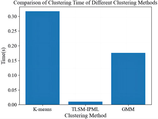
Figure 5. Comparison of clustering time of different clustering methods.

Figure 6

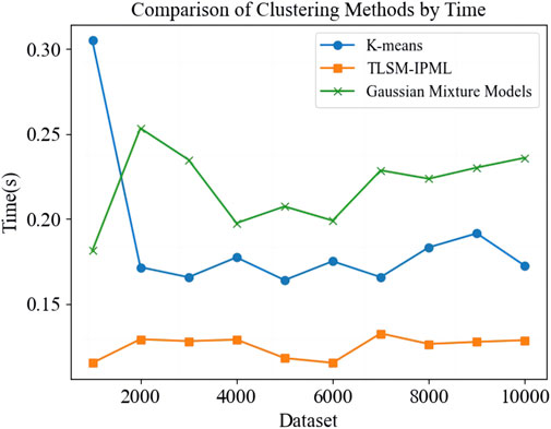
Figure 6. Comparison of clustering methods by time.

The simulation experimental results show that the TLSM-IPML algorithm has good clustering results for the real load data used in the experiments and can maintain smooth changes in the clustering results. The experimental results also show that TLSM-IPML can well-portray the changing trend of users’ load profiles.

4 Planning model of MES

After completing the simulation of all types of equipment, bus-wise load profiles are created over a period of 10 years. A new objective function that motivates the seasonal hydrogen energy storage is proposed in this work. The net costs of the hydrogen system, PV system, ESS (energy storage system), and grid power define the objective function of the optimization problems to be minimized.

4.1 Objective function

In the multi-objective optimization of the integrated energy system, the objective functions for minimizing total cost $F_{\mathit{all}}$ and carbon emission $F_c$ are combined using a weighted sum: $F={\omega }_1{F}_{\mathit{all}}+{\omega }_2{F}_c$. Selecting appropriate initial weights ${\omega }_1$ and ${\omega }_2$ involves expert knowledge, sensitivity analysis, iterative adjustment, and normalization. Dynamic weight adjustment ensures the model’s adaptability to complex planning scenarios.

To validate the impact of different weight values (${\omega }_1$ and ${\omega }_2$) on the optimization results, we conduct experiments using the integrated energy system model of the heavy equipment manufacturing industrial park. The objective functions considered are total costs $(F_{\mathit{all}})$ and carbon emissions $(F_c)$.

4.1.1 Lowest total costs

A new objective function that motivates the seasonal hydrogen energy storage is proposed in this work. The net costs of the hydrogen system, PV system, ESS, and grid power are considered to define the objective function of the optimization problem that is to be minimized.

$min{F}_{\mathit{all}}=min\left\{F_{\mathit{inv}}+F_{\mathit{ope}}+F_{\mathit{deg}}+F_{be}-F_{pe}\right\}.(21)$

The objective function in Equation 21 represents five system cost components which describe the system net cost of the industrial integrated energy system, which is given as follows: 1) total capital expenditure, as shown in Equation 22; 2) total operating expenses, including maintenance and environmental costs, as shown in Equation 23; 3) degradation costs of the ESS and electrolyzer system, as shown in Equation 27; 4) energy purchasing costs, as shown in Equation 28); and 5) benefits from energy production, as shown in Equation 29. In this work, the electricity price ($J_{E,m}^t$) considers the variable and fixed charges. The grid cost in Equation 28 is multiplied by the Z-score of the historical set of electricity prices, $T^H=\left\{\mathrm{1,2},\dots ,t^h,\dots ,t\right\}$, that serves as a reward or penalty for seasonal storage application purposes. The value of the Z-score shows how far the current electricity price at time $t$ is.

$F_{\mathit{inv}}={\displaystyle \sum _{i=1}^I}{\alpha }_i^P{C}_i^P,(22)$

where i is the number of equipment types; I is the number of equipment; $C_i^P$ is the capacity of equipment i; and ${\alpha }_i^P$ is the installation cost per unit capacity.

$F_{\mathit{ope}}=F_{\mathit{Main}}+F_{\mathit{Env}},(23)$

$F_{\mathit{Main}}={\displaystyle \sum _{s=1}^S}{D}_s{\displaystyle \sum _{t=1}^T}{\displaystyle \sum _{i=1}^I}{\beta }_i{\varphi }_i^t\mathrm{\Delta }t+{\displaystyle \sum _{i=1}^n}{z}_t^i{C}_{t_i^0,t}^i{P}_{i,equ}^t,(24)$

where s is typical days; S is the number of typical days; $D_s$ is the number of days for typical days; T is the scheduling cycle, which is taken as 24 h; ${\beta }_i$ is the operation and maintenance costs per unit output of equipment $i$; ${\varphi }_i^t$ is the output of equipment $i$ in period $t$; $C_{i,ope}$ is the operation and maintenance costs of large energy-consuming equipment in the heavy equipment manufacturing industry; and $P_{i,equ}$ is the EC of large energy-consuming equipment, kW, which is proposed in Eq.(15).

The last term of Equation 24, the maintenance cost of the energy consumption types of equipment, corresponds to the dynamic maintenance cost associated with equipment maintenance. Notably, the dynamic maintenance costs $C_{t_i^o,t}^i$ are computed from the remaining life distributions of operating energy-consuming equipment, which are updated based on sensor observations. The dynamic maintenance cost function quantifies the tradeoff between the cost of preventive action and the risk of unexpected failures by defining their corresponding probabilities through the sensor-updated remaining life estimates. The dynamic maintenance cost is represented as follows Equation 25:

$C_{t_i^o,t}^i=\frac{c_i^{p}P\left(R_{t_i^o}^i>t\right)+c_i^{f}P\left(R_{t_i^0}\le t\right)}{{\int }_0^{t}P\left(R_{t_i^o}>z\right)dz+t_i^o},(25)$

where $C_{t_i^o,t}^i$ represents the cost rate associated with conducting energy-consuming equipment maintenance $t$ periods after the time of observation $t_i^0$; $c_i^p$ and $c_i^f$ are the costs of planned maintenance and failure replacement, respectively. The dynamic maintenance cost (24) uses renewal reward to characterize the long-run expected maintenance cost. The numerator evaluates the expected cost of maintenance, where the terms $c_i^{p}P(R_{t_i^o}^i>t)$ and $c_i^{f}P(R_{t_i^0}\le t)$ represent the expected cost of preventive and corrective actions, respectively. The denominator, on the other hand, represents the expected length of the cycle. The first term, ${\int }_0^{t}P(R_{t_i^o}>z)dz$, finds the expected remaining lifetime of the component, given that preventive maintenance is planned at time $t$, and $t_i^o$ is the deterministic time of observation that is already a part of the current cycle.

$F_{\mathit{Env}}={\displaystyle \sum _{s=1}^S}{D}_s{\displaystyle \sum _{t=1}^T}\gamma \left({\epsilon }_E{P}_{\mathit{Grid}}^t+{\epsilon }_G{V}_{\mathit{GasPip}}^t\right)\mathrm{\Delta }t,(26)$

In Equation 26, where $\gamma$ is the carbon tax, which is taken as 0.02 (Yuan/kg) in this paper; ${ϵ}_E$ and ${ϵ}_G$ are the carbon emission coefficients of the park’s purchased electricity and natural gas, respectively; $P_{\mathit{Grdi}}^t$ is the electric power purchased by the system during period t; and $V_{\mathit{GasPip}}^t$ is the amount of natural gas purchased by the system from the gas grid during period t, $m^3$.

$F_{\mathit{deg}}={\displaystyle \sum _{s=1}^S}{D}_s{\displaystyle \sum _{t=1}^T}{D}_{BS}^t\cdot \left(P_{BS,Chg}^t+P_{BS,Dhg}^t\right)+D_{\mathit{Elz}}^t\cdot P_{\mathit{Elz}}^t,(27)$

where $D_t^{BS}$ is the ESS degradation cost (Yuan/MW); $p_t^{BS,Chg}$ is the ESS charging power (MW); $p_t^{BS,Dhg}$ is the ESS discharging power (MW); $D^{\mathit{Elz}}$ is the electrolyzer stack replacement cost (Yuan/MWh); and $p_t^{\mathit{Elz}}$ is the electrolyzer input power (MW).

$\begin{array}{ll}\hfill F_{be}& ={\displaystyle \sum _{s=1}^S}{D}_s{\displaystyle \sum _{t=1}^T}\left(J_{E,m}^t{P}_{\mathit{Grid}}^t\cdot Z_t^e+J_{G,m}^t{V}_{\mathit{GasPip}}^t\right.\hfill \\ \hfill & \left.+J_{H,m}^t{Q}_{\mathit{Heat}}^t+J_{Hy,m}{V}_{Hy,m}^t\right)\mathrm{\Delta }t,\hfill \end{array}(28)$

$F_{pe}={\displaystyle \sum _{s=1}^S}{D}_s{\displaystyle \sum _{t=1}^T}\left(P_g^t{J}_{E,m}^t+J_{H,m}{Q}_g^t+J_{G,m}{V}_g^t+J_{Hy,m}{V}_{Hy,m}^t\right)\mathrm{\Delta }t.(29)$

The objective function is subjected to the operational and capacity constraints, as discussed herein.

4.1.2 Lowest carbon emissions

The objective function for the lowest carbon emission is as shown in following Equation 30:

$F_c=y{\displaystyle \sum _{i=1}^n}{x}^i{N}^i,(30)$

where $F_c$ is the total carbon emissions during the entire life cycle; $y$ is the entire system life cycle; $n$ is the optimal number of planned devices; and $N_i$ is the carbon emissions of the $i$th device in a unit period.

4.2 Constraints

1) ESS constraints: Similar to the HS, the ESS has operational constraints that ensure a safe operation of the ESS. The ESS operation is subjected to maximum and minimum limits, as shown to avoid excessive charging and discharging that can damage the ESS as following Equations 31, 32:

$P_{\mathit{min}}^{ES,Chg}⩽P_t^{ES,Chg}⩽P_{\mathit{max}}^{ES,Chg},(31)$

$P_{\mathit{min}}^{ES,Dhg}⩽P_t^{ES,Dhg}⩽P_{\mathit{max}}^{ES,Dhg}.(32)$

In order to minimize power lost during charging and discharging due to process efficiencies, constraints in Equation 33 are included to prevent simultaneous charging and discharging as

$P_t^{ES,Chg}\cdot P_t^{ES,Dhg}=0.(33)$

2) System power balance: The amount of power purchased from the power grid is limited by the maximum and minimum grid operational capabilities as follows:

$P_{\mathit{min}}^{\mathit{Grid}}⩽p_t^{\mathit{Grid}}⩽P_{\mathit{min}}^{\mathit{Grid}}.(34)$

5 Case study

In this section, the sources of data, including equipment parameters and park scale, are introduced in Section 5.1. In addition, this section conducts a data clustering experiment (Section 5.2) to analyze typical day energy consumption in the heavy equipment manufacturing park using TLSM-IPML. Section 5.3 analyzes the impact of different equipment inputs on energy system planning through five scenarios and examines how varying fuzzy membership weights affect the planning results.

5.1 Data source and park scale

Simulations validated the MES model for cost minimization in a large industrial park. The 2-sq km park with 50+ facilities has a 200-MW capacity, 150 MW peak demand, and consumes 1.2 TWh electricity and 0.8 TWh thermal energy annually. It features substations, on-site generation, backup generators, and a natural gas system. Cooling is done by 50,000 RT chillers, and heating is done by 100-MW gas boilers and heat exchangers. Renewables include 30-MW solar PV, 20-MW wind, 50-MWh battery, and thermal storage.

The MES model integrates hydrogen production, PV, wind turbines, CCHP, heat turbines, waste heat recovery, and ESS, optimizing with real-time electricity prices from Sichuan Province ESO. Electrolyzer size is tailored for 70$\%$ annual operation to maximize economic benefits (El-Taweel et al., 2019).

Wind resources are favorable with an annual average speed of 7.3 m/s and power density of 382 W/m². Photovoltaic data indicate moderate potential for investment, with scattered radiation and stable conditions, albeit lower economic returns compared to wind power.

5.2 Comparing TlSM-IPML with other methods

In this section, we compare our algorithm with the K-means algorithm. The performance of the proposed algorithm is verified through experiments on real-world benchmark datasets. We conducted a comparative study with existing clustering methods including K-means and A-MKMC, as shown in Figures 7, 8. The results of the A-MKMC clustering method applied to the 8,760 electric load data points are presented in Figure 8, representing Level 1 and Level 2 of hierarchical clustering. Although the data points remain identical, the hierarchical clustering approach differentiates the figures by their levels of granularity. Level 1 clustering identifies broader clusters that capture general load patterns, while Level 2 clustering refines these into more specific subgroups. This hierarchical method allows for a detailed analysis of load profiles, offering a comprehensive understanding which is essential for accurate energy planning and management in industrial parks. The comprehensive analysis of the results of K-means and A-MKMC clustering methods shows that the load situation in the park is roughly divided into four cluster centers, which can be understood as the four load situations corresponding to the four working conditions in the park. However, based on this clustering result, it is impossible to analyze the load relationship between different typical days, which is not conducive to analyzing the load situation of the park in different months and seasons.

Figure 7

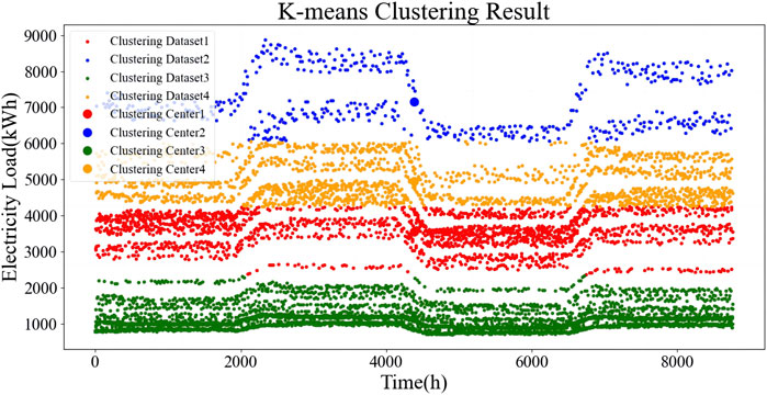
Figure 7. K-means clustering result.

Figure 8

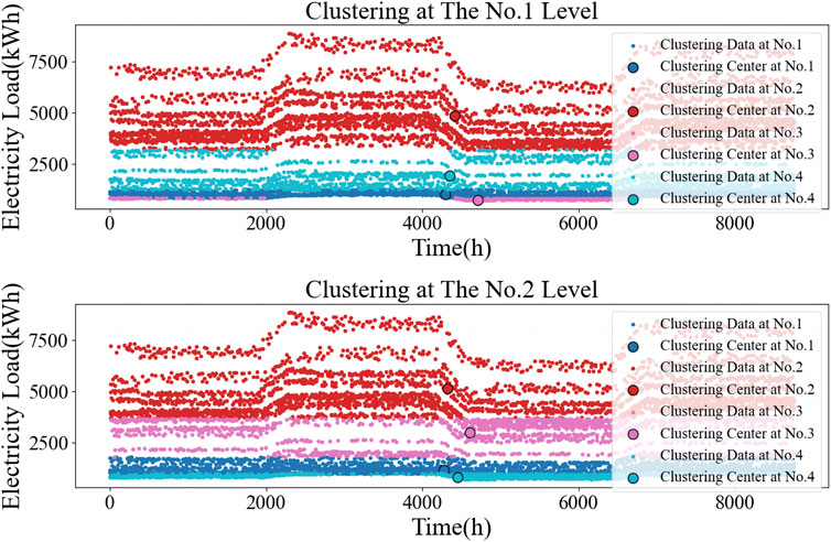
Figure 8. A-MKMC clustering result.

In Figure 9, TLSM-IPML shows a significant shift in electricity consumption behavior on different days, which traditional clustering methods do not capture. Figure 10 analyzes two seasons of consumption data, highlighting TLSM-IPML’s ability to track evolving patterns over time. Our TLSM-IPML method achieves higher clustering accuracy and better captures the load variation patterns specific to heavy equipment manufacturing. When the behavior is stable, TLSM-IPML maintains historical data for consistent clusters. Yet, significant changes prompt adaptive clustering, potentially yielding new outcomes.

Figure 9

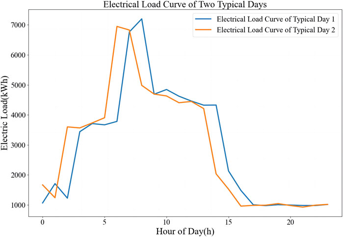
Figure 9. Electric load curves of two selected typical days.

Figure 10

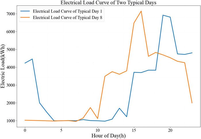
Figure 10. Comparison of load data for two typical days in spring and summer.

To further validate our proposed method, we have included an additional dataset from one different industrial park. The dataset covers a range of operational conditions and energy consumption patterns. Figure 11 illustrates the application of the clustering method on the new datasets, demonstrating its robustness and versatility.

Figure 11

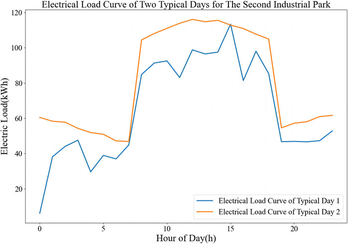
Figure 11. Electrical load curve of two typical days for the second industrial park.

The peaks and valleys in the load diagram offer insights into the daily variations in electricity usage. To enhance the understanding of energy consumption behavior, additional information can be extracted from these load diagrams through further analysis.

• Identifying peak load hours is vital for operational planning and load shifting. For instance, in one dataset, demand rises from 8 a.m., peaks at 1 p.m., declines until 8 p.m., and stays low until 5 a.m. the next day. Pinpointing low-energy periods aids in scheduling maintenance and optimizing energy use.

• Categorizing days by load profiles (weekdays vs weekends and production vs non-production) reveals operational impacts on energy use. Weekdays peak around 2 p.m. and weekends at 11 a.m. Seasonal analysis shows summer peaks from 11 a.m. to 5 p.m. and winter from 3 p.m. to 7 p.m., guiding energy strategies.

• Calculating energy intensity highlights industrial efficiency. High production days may reach 1.5 kWh per unit, and low production days may reach up to 2.0 kWh per unit, indicating inefficiencies. The average load factor is 0.75 and stable with potential for improvement on 0.6 factor days.

• Analyzing load diagrams predicts future trends. For example, summers typically see a 5$\%$-peak load increase, aiding proactive energy management. Anomaly detection, like 10 p.m. spikes, prompts timely maintenance to prevent disruptions.

Load diagrams from TLSM-IPML clustering reveal that peaks and valleys pinpoint high-demand times and load-shifting opportunities while classifying load profiles, seasonal variations, and metrics like energy intensity and load factor optimize usage insights.

5.3 Performance analysis of the planning model

Five cases (Table 4) compare different configurations, highlighting base cases (case 1 and case 5) for analysis.

Table 4

Table 4. Test cases.

Tables 5, 6 reveal that annual total costs significantly decrease after equipment planning. For instance, comparing case 1 withcase 5, costs drop by 48.26$\%$, a reduction of 31.357 million CNY annually. Savings stem from photovoltaic planning, enabling the park to generate electricity using clean energy, replacing higher-cost purchases. Battery planning allows peak shifting, reducing electricity costs during peak hours. Ground source heat pump planning reduces electricity-to-heat conversion costs.

Table 5

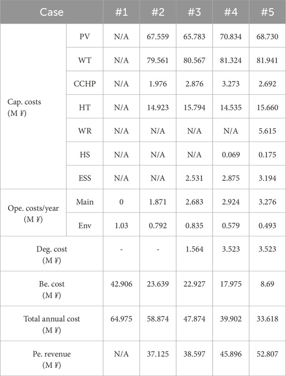
Table 5. Economic optimization results of the IES under each case.

Table 6

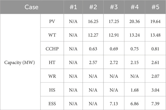
Table 6. Capacity optimization results of the IES under each case.

The proposed MES involves key parameters influencing optimization results. Further analysis examines the impact of PV generation share on energy conversion efficiency. Setting the Z-score of historical electricity prices to 1 in cases 3 and 4 reduces annual costs by 7.97 million CNY, a 16.65$\%$ decrease compared to non-use scenarios. This underscores the necessity of seasonal hydrogen storage equipment in industrial energy system planning, demonstrating economic benefits and system flexibility through electrolytic hydrogen and hydrogen storage technologies. The conclusions from the case study analysis are as follows: 1) comprehensive energy planning significantly reduces park operating costs and annual fees; 2) ground-source heat pumps are valuable for adapting to fluctuating natural gas and electricity prices; 3) electric energy storage is beneficial despite price fluctuations, effectively lowering park operational costs.

We selected two sets of weight values to explore their effects on the optimization outcome. The weight values are shown in Table 7. In addition, the optimization results for each set of weight values are summarized in Table 8. Optimization with a higher cost weight minimizes total costs to 437.097 M CNY but increases emissions to 468.034 $m^3$. Prioritizing emission minimization raises costs to 561.273 M CNY while achieving lower emissions at 153.345 $m^3$, illustrating the trade-off between the cost and environmental impact.

Table 7

Table 7. Selection of weight values.

Table 8

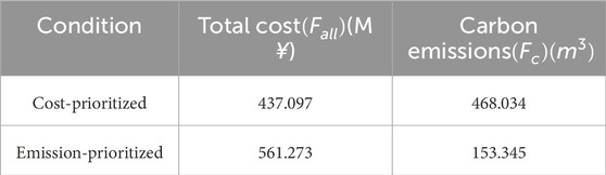
Table 8. Optimization results for each set of weight values.

The study shows that weight values significantly influence optimization outcomes. Decision-makers should select weights based on priorities; higher ${\omega }_1$ values prioritize emission reduction, which is crucial for regulatory compliance or sustainability goals, while higher ${\omega }_2$ values focus on cost reduction.

6 Conclusion

This study proposes an integrated planning approach for the energy systems of heavy equipment manufacturing industrial parks. By combining ARIMA and temporal convolutional networks (TCNs), we developed an advanced model that accurately predicts the energy consumption of heavy equipment, capturing both temporal dependencies and non-linear characteristics. Utilizing the TLSM-IPML method, we identified representative load days that reflect the diverse energy consumption patterns in the industrial park, improving the accuracy and effectiveness of energy system planning. Integrating the predictive energy consumption model and typical load days, we designed a comprehensive planning model that optimizes energy usage and minimizes operational costs by considering the unique characteristics of heavy equipment operations. Overall, our integrated approach enhances the efficiency and cost-effectiveness of energy system planning in heavy equipment manufacturing industrial parks. Future work will focus on refining these models and exploring their application in different industrial contexts to further validate their robustness.

Data availability statement

The original contributions presented in the study are included in the article/Supplementary Material; further inquiries can be directed to the corresponding author.

Author contributions

DC: conceptualization, data curation, investigation, methodology, resources, software, validation, writing–original draft, and writing–review and editing. QC: writing–review and editing. DL: writing–review and editing. PR: resources and writing–review and editing.

Funding

The authors declare that no financial support was received for the research, authorship, and/or publication of this article.

Conflict of interest

Author PR was employed by Dongfang Electric Group Dongfang Electric Motor Co., Ltd.

The remaining authors declare that the research was conducted in the absence of any commercial or financial relationships that could be construed as a potential conflict of interest.

Publisher’s note

All claims expressed in this article are solely those of the authors and do not necessarily represent those of their affiliated organizations, or those of the publisher, the editors, and the reviewers. Any product that may be evaluated in this article, or claim that may be made by its manufacturer, is not guaranteed or endorsed by the publisher.

References

Araghian, M. H., Rahimiyan, M., and Zamen, M. (2023). Robust integrated energy management of a smart home considering discomfort degree-day. IEEE Trans. Industrial Inf. 19, 10133–10144. doi:10.1109/TII.2023.3234083

CrossRef Full Text | Google Scholar

Chauhan, A., and Saini, R. P. (2014). “Statistical analysis of wind speed data using weibull distribution parameters,” in 2014 1st international conference on non conventional energy (ICONCE 2014), 160–163. doi:10.1109/ICONCE.2014.6808712

CrossRef Full Text | Google Scholar

Chen, Y., Tang, S., Pei, S., Wang, C., Du, J., and Xiong, N. (2018). Dheat: a density heat-based algorithm for clustering with effective radius. IEEE Trans. Syst. Man, Cybern. Syst. 48, 649–660. doi:10.1109/TSMC.2017.2745493

CrossRef Full Text | Google Scholar

Cheng, D., Zhu, Q., Huang, J., Wu, Q., and Yang, L. (2021). Clustering with local density peaks-based minimum spanning tree. IEEE Trans. Knowl. Data Eng. 33, 374–387. doi:10.1109/TKDE.2019.2930056

CrossRef Full Text | Google Scholar

Clegg, S., and Mancarella, P. (2016). Integrated electrical and gas network flexibility assessment in low-carbon multi-energy systems. IEEE Trans. Sustain. Energy 7, 718–731. doi:10.1109/TSTE.2015.2497329

CrossRef Full Text | Google Scholar

El-Taweel, N. A., Khani, H., and Farag, H. E. Z. (2019). Analytical size estimation methodologies for electrified transportation fueling infrastructures using public–domain market data. IEEE Trans. Transp. Electrification 5, 840–851. doi:10.1109/TTE.2019.2927802

CrossRef Full Text | Google Scholar

Fan, W., Bouguila, N., Du, J.-X., and Liu, X. (2019). Axially symmetric data clustering through dirichlet process mixture models of watson distributions. IEEE Trans. Neural Netw. Learn. Syst. 30, 1683–1694. doi:10.1109/TNNLS.2018.2872986

PubMed Abstract | CrossRef Full Text | Google Scholar

Fan, W., Sallay, H., and Bouguila, N. (2017). Online learning of hierarchical pitman–yor process mixture of generalized dirichlet distributions with feature selection. IEEE Trans. Neural Netw. Learn. Syst. 28, 2048–2061. doi:10.1109/TNNLS.2016.2574500

PubMed Abstract | CrossRef Full Text | Google Scholar

Fang, X., Xu, Z., Ji, H., Wang, B., and Huang, Z. (2023). A grid-based density peaks clustering algorithm. IEEE Trans. Industrial Inf. 19, 5476–5484. doi:10.1109/TII.2022.3203721

CrossRef Full Text | Google Scholar

Fu, C., Lin, J., Song, Y., Li, J., and Song, J. (2020). Optimal operation of an integrated energy system incorporated with hcng distribution networks. IEEE Trans. Sustain. Energy 11, 2141–2151. doi:10.1109/TSTE.2019.2951701

CrossRef Full Text | Google Scholar

Good, N., and Mancarella, P. (2019). Flexibility in multi-energy communities with electrical and thermal storage: a stochastic, robust approach for multi-service demand response. IEEE Trans. Smart Grid 10, 503–513. doi:10.1109/TSG.2017.2745559

CrossRef Full Text | Google Scholar

Li, J., Lin, J., Song, Y., Xing, X., and Fu, C. (2019). Operation optimization of power to hydrogen and heat (p2hh) in adn coordinated with the district heating network. IEEE Trans. Sustain. Energy 10, 1672–1683. doi:10.1109/TSTE.2018.2868827

CrossRef Full Text | Google Scholar

Lv, Z., Kong, W., Zhang, X., Jiang, D., Lv, H., and Lu, X. (2020). Intelligent security planning for regional distributed energy internet. IEEE Trans. Industrial Inf. 16, 3540–3547. doi:10.1109/TII.2019.2914339

CrossRef Full Text | Google Scholar

Mahran, S., and Mahar, K. (2008). “Using grid for accelerating density-based clustering,” in 2008 8th IEEE international conference on computer and information Technology, 35–40. doi:10.1109/CIT.2008.4594646

CrossRef Full Text | Google Scholar

Martínez Cesena, E. A., and Mancarella, P. (2019). Energy systems integration in smart districts: robust optimisation of multi-energy flows in integrated electricity, heat and gas networks. IEEE Trans. Smart Grid 10, 1122–1131. doi:10.1109/TSG.2018.2828146

CrossRef Full Text | Google Scholar

Mehrjerdi, H., Hemmati, R., Shafie-khah, M., and Catalão, J. P. S. (2021). Zero energy building by multicarrier energy systems including hydro, wind, solar, and hydrogen. IEEE Trans. Industrial Inf. 17, 5474–5484. doi:10.1109/TII.2020.3034346

CrossRef Full Text | Google Scholar

Muja, M., and Lowe, D. G. (2014). Scalable nearest neighbor algorithms for high dimensional data. IEEE Trans. Pattern Analysis Mach. Intell. 36, 2227–2240. doi:10.1109/TPAMI.2014.2321376

PubMed Abstract | CrossRef Full Text | Google Scholar

Pombo, D. V., Martinez-Rico, J., Carrion, M., and Cañas-Carretón, M. (2023). A computationally efficient formulation for a flexibility enabling generation expansion planning. IEEE Trans. Smart Grid 14, 2723–2733. doi:10.1109/TSG.2022.3233124

CrossRef Full Text | Google Scholar

Rhodes, J. D., Cole, W. J., Upshaw, C. R., Edgar, T. F., and Webber, M. E. (2014). Clustering analysis of residential electricity demand profiles. Appl. Energy 135, 461–471. doi:10.1016/j.apenergy.2014.08.111

CrossRef Full Text | Google Scholar

Shao, M., Liu, J., Yang, Q., Shen, B.-Z., and Wu, M. (2023). Fog node planning with stochastic sensor traffic in dynamic industrial environment. IEEE Trans. Industrial Inf. 19, 9217–9226. doi:10.1109/TII.2022.3227634

CrossRef Full Text | Google Scholar

Yodwong, B., Guilbert, D., Phattanasak, M., Kaewmanee, W., Hinaje, M., and Vitale, G. (2020). Faraday’s efficiency modeling of a proton exchange membrane electrolyzer based on experimental data. ENERGIES 13, 4792. doi:10.3390/en13184792

CrossRef Full Text | Google Scholar

Zeng, B., Zhang, J., Yang, X., Wang, J., Dong, J., and Zhang, Y. (2014). Integrated planning for transition to low-carbon distribution system with renewable energy generation and demand response. IEEE Trans. Power Syst. 29, 1153–1165. doi:10.1109/TPWRS.2013.2291553

CrossRef Full Text | Google Scholar

Zhang, B., Zhang, L., Wang, Z., Cui, Z., Sun, Y., and Hua, H. (2023). Image reconstruction of planar electrical capacitance tomography based on dbscan and self-adaptive admm algorithm. IEEE Trans. Instrum. Meas. 72, 1–11. doi:10.1109/TIM.2023.3284931

PubMed Abstract | CrossRef Full Text | Google Scholar

Zhang, D., Zhu, H., Zhang, H., Goh, H. H., Liu, H., and Wu, T. (2021). Multi objective optimization for smart integrated energy system considering demand responses and dynamic prices. IEEE Trans. Smart Grid 13, 1100–1112. doi:10.1109/TSG.2021.3128547

CrossRef Full Text | Google Scholar

Zhao, Y., Wang, C., Zhang, Z., and Lv, H. (2021). Flexibility evaluation method of power system considering the impact of multi-energy coupling. IEEE Trans. Industry Appl. 57, 5687–5697. doi:10.1109/TIA.2021.3110458

CrossRef Full Text | Google Scholar

Zhong, W., Xie, K., Liu, Y., Yang, C., and Xie, S. (2018). Auction mechanisms for energy trading in multi-energy systems. IEEE Trans. Industrial Inf. 14, 1511–1521. doi:10.1109/TII.2017.2787751

CrossRef Full Text | Google Scholar