Frequency minimum inertia calculation of complex power systems based on an improved simulated annealing algorithm

In order to enhance the inertia situational awareness and stability of the power system in the context of the reduction of power system inertia and the challenge of frequency stability due to the high proportion of new energy access, the background and purpose of the study are stated in the introduction; methodologically, based on the frequency response model of the power system, we analyze the time and magnitude of the maximum frequency offset, clarify the factors affecting the frequency stability and construct the mathematical relationship, and then build a model for assessing the minimum inertia of the power system taking into account the virtual inertia of the new energy source. Then, based on the whole process of frequency response, we construct a power system minimum inertia assessment model taking into account the virtual inertia of new energy sources, and introduce an improved simulated annealing algorithm to solve the problem; the results validate the accuracy of the method through the IEEE-14 node model; the discussion section points out that this method provides a feasible solution for the inertia situational awareness of power system, which is helpful for the optimization of the operation, and also proposes that in the future we can take into account more uncertainties to improve the model and algorithm and to enhance the practicability and adaptability of this method. It is also suggested that more uncertainty factors can be considered in the future to improve the model and algorithm and enhance the practicality and adaptability.

1 Introduction

Motivated by China’s ambition to achieve the “dual carbon” targets, the development of wind and photovoltaic power generation is poised for significant progress (Zhang et al., 2019). It is projected that by 2030, the installed capacity of renewable energy sources, including wind and photovoltaic systems, will escalate 1.07–1.27 TW, resulting in a total installed capacity reaching 1.6–1.8 TW (Huadong et al., 2024). However, the lack of inertia in the new power system poses a substantial threat to its operation due to its inability to provide reliable primary frequency modulation support for the system as do traditional synchronous generating units such as thermal power and hydropower (Zimin et al., 2023; Fu et al., 2023). This challenge is intensifying as the proportion of renewable energy generation in the system grows, underscoring the need for more in-depth research into minimum inertia requirements for future advancements (Song et al., 2023; Zhang et al., 2021).

At present, the evaluation of system inertia requirements by researchers around the world is mostly carried out based on the rate of change of frequency (RoCoF) and frequency deviation constraints. For power systems with a high proportion of new-energy power generation, a method for evaluating the minimum inertia of a wind-storage combined frequency modulation power system is proposed. An equivalent inertia index considering the participation of multiple resources is also proposed, and the factors affecting the minimum inertia of the system are quantified (Yunfeng and Huangxiao, 2021). Some scholars define the power-system frequency stability index as the ratio of the actual operating inertia of the current power system to the critical inertia level, and thereby obtain the virtual inertia compensation amount that new-energy power generation units need to service the system (Shichun et al., 2025).

There are numerous complex challenges in the field of inertia calculation. As stated in Ruyin et al. (2025), the parameters of various components in the power grid are uncertain, which raises the problem of basic data errors in inertia calculation. The differences in the aging degree and manufacturing processes of different devices make it difficult to accurately determine parameters, thus affecting the accuracy of inertia calculation. According to Zhiyong et al. (2025), with the large-scale integration of distributed energy sources, it is difficult to adapt traditional centralized inertia calculation methods to the dispersed and variable characteristics of distributed power sources or to accurately integrate the contributions of distributed power sources at different locations to the system inertia. In addition, as proposed in Jiebei et al. (2024), multiple physical processes in the power system, such as electromagnetic transients and electromechanical transients, all need to be considered when establishing an inertia calculation model. According to Zhenhao et al. (2024), the convergence curve is calculated by the imperialist competition algorithm (ICA); by simulating the competition and assimilation mechanism among the “empires,” the convergence rate is faster in the optimization process (Pratap et al., 2023). The strategy of using a hybrid whale optimization algorithm (WOA) and simulated annealing (SA) combines the global exploration capability of WOA with the local development capability of SA. In 90% of cases, the convergence accuracy is better than the original WOA and m-WOA, and the convergence curve is smoother, especially when dealing with high-dimensional, multi-modal problems. The limitation of the current study is that the role of the virtual inertia of new energy generating units on the generation side is not considered, while the constraints set by the evaluation model do not consider the handling constraints of the generating units. It is thus necessary to construct a complete and accurate evaluation model of the minimum inertia of the power system.

In order to solve this problem, we propose a model for calculating the minimum inertia demand of a power system. The model establishes a detailed power system frequency response model, including virtual inertia, by considering that the frequency problem is affected by many factors. On this basis, a minimum inertia optimization model containing RoCoF constraints is established and solved by an improved simulated annealing algorithm, which can quickly obtain the results of inertia demand assessment.

2 Frequency response model of a power system

2.1 System frequency response mechanism

In scenarios involving power outages, load reductions, or abrupt changes in load active power, the balance between a system’s active power and frequency is disrupted. The response process of the system frequency can be categorized into inertia response, primary frequency modulation, secondary frequency modulation, and distribution optimization based on the time scale order (Patricia et al., 2024; Shetty and Chakrasali, 2021).

When there is a disruption in the system, the initial response comes from the stored inertia within it. The alternator, equipped with the moment of inertia, plays a crucial role in stabilizing system frequency and preventing fluctuations. Upon occurrence of an active power imbalance, the first line of defense is provided by a system’s inertia response. The kinetic energy stored in synchronous generators with the moment of inertia is then either released or absorbed based on individual generator inertia, effectively minimizing unbalanced power and maintaining system frequency stability. At the moment of $t_{gov}$, the system performs an FM system response. Upon exceeding the lower threshold of the dead zone for frequency deviation, the governor initiates a signal to modulate the prime mover valve, thereby augmenting the mechanical power output from the generator. If the primary frequency modulation system has enough capacity, the unit’s active power output will continue to rise, gradually restoring system frequency until it reaches a stable state (Lin et al., 2021; Xia et al., 2018). The rotor motion equation of the system is shown as Formula 1

$2H_G\frac{d\Delta f\left(t\right)}{dt}+D\Delta f\left(t\right)=\Delta P_g+\Delta P_m+\Delta P_d,(1)$

where $\Delta P_d$ is the active power disturbance of the system load, $H_g$ is the inertia time constant of synchronous generator set, $\Delta f\left(t\right)$ is the frequency disturbance of the system, $\Delta P_m$ is the primary frequency modulation adjustment amount involved in the virtual inertia of new energy, $\Delta P_g$ is the synchronous generator system to restore stable adjustment power, and $D$ is the damping coefficient of the system.

2.2 System frequency response model

To enhance the frequency response capability of the new energy generator set, the converter control strategy was enhanced to provide inertia response and match the external characteristics of synchronous generators. New energy virtual inertia sources come in various forms, such as static energy storage and fan rotational kinetic energy, which effectively offer instant power support and mitigate rapid frequency changes during disturbances (Mercier et al., 2009; Yefeng et al., 2024).

The system frequency response model for the power system with new energy sources is constructed using an equivalent method, which includes both the traditional thermal power generation primary frequency modulation system and the new energy virtual inertia primary frequency modulation system. In order to simplify the model, only the reheat time constant is considered due to the much smaller time constants of the governor and steam box. Additionally, a low-order model is used in the primary frequency modulation system.

Upon examining the conventional power system frequency response model, the frequency response formulation for a system incorporating new energy generation participating in primary frequency regulation can be expressed as shown in Formula 2

${\Delta }_Z=\left(\frac{R{Z}_1^2}{DR+g_n}\right)\left(\frac{g_n\left(1+F_H{T}_{\mathrm{r}}^{q}s\right)P_{sp}-\left(1+T_{\mathrm{r}}^{q}s\right)P_e}{s^2+2\phi Z_{1}s+Z_1^2}\right).(2)$

In the above formula, as shown in Formula 3

$\begin{array}{l}\left\{\begin{array}{l}{Z}_1^2=\frac{DR+{\mathrm{g}}_n}{2H_{all}R{T}_q^r},\\ \phi =\left[\frac{2H_{all}R+\left(DR+{\mathrm{g}}_n{F}_H\right)T_q^r}{2\left(DR+{\mathrm{g}}_n\right)}\right]Z_1,\end{array}\right.\\ H_{all}=H+H_{new},\end{array}(3)$

where $H$ is the inertia time constant of the generator, $H_{new}$ is the virtual inertia constant of the new energy generator set, $D$ is the equivalent damping coefficient of the generator, $R$ is the adjustment factor of the governor, $T_q^r$ is the reheat time constant of the prime mover, $F_H$ is the work ratio of the high pressure cylinder of the prime mover, ${\mathrm{g}}_n$ is the coefficient related to the generator power factor and reserve capacity, $P_m$ is the output power for the prime mover, $P_e$ is the load power, $P_{sp}$ adds power to the generator, ${\Delta }_z$ indicates the deviation of the average system speed, s indicates the rated capacity of the unit, and $Z_1$ is the intermediate variable to simplify the calculation.

As shown in Figure 1 analyzing the frequency response model, only the change of $P_e$ is considered, and the change of $P_{sp}$ is not. Formula 4 is thus simplified:

${\Delta }_Z=\left(\frac{R{Z}_1^2}{DR+{\mathrm{g}}_{\mathrm{n}}}\right)\left(\frac{\left(1+F_H{T}_r^{q}s\right)P_d}{s^2+2\phi z_{1}s+z_1^2}\right).(4)$

Figure 1

Figure 1. Frequency response model of a power system.

Utilizing the inverse Laplace transform, the time-domain representation of the frequency deviation can be derived as follows:

${\Delta }_{Z\left(t\right)}=\left(\frac{R{z}_1^2}{DR+g_n}\right)\left[1+{\alpha }^{-\delta z_1}\sin \left(z_{2}t+\phi \right)\right],(5)$

As shown in Formulas 6–10

$Z_1^2=\frac{DR+g_n}{2HR{T}_q^r},(6)$

$\delta =\left[\frac{2HR+\left(DR+{\mathrm{g}}_n{F}_H\right)T_q^r}{2\left(DR+g_n\right)}\right]z_1,(7)$

$\delta =\left[\frac{2HR+\left(DR+{\mathrm{g}}_n{F}_H\right)T_q^r}{2\left(DR+g_n\right)}\right]z_1,(8)$

$Z_2=Z_1\sqrt{1-{\delta }^2,}(9)$

$\phi ={\phi }_1-{\phi }_2={\tan }^{-1}\left(\frac{z_2{T}_q^r}{1-\delta z_1{T}_q^r}\right)-{\tan }^{-1}\left(\frac{\sqrt{1-{\delta }^2}}{-\delta }\right).(10)$

Assuming that the magnitude of the disturbance is ${\Delta }_P$, the time-domain frequency representation of the system under the influence of a disturbance as shown in Formula 11

$\begin{array}{l}{t}_n=\frac{1}{\mathrm{\Omega }}{\tan }^{-1}\left(\frac{{\mathrm{\Omega }}_r{T}_r^q}{\delta {\mathrm{\Omega }}_n{T}_r^q-1}\right),\\ \Delta f_n=\Delta f\left(t_n\right).\end{array}(11)$

Since the maximum value ${\frac{d\Delta f}{dt}}_{\max }$ of the frequency change rate is obtained at time t = 0, the frequency deviation is 0, so the system output is also 0. The size of ${\frac{d\Delta f}{dt}}_{\max }$ as shown in Formula 12

${\left(\frac{d\Delta f}{dt}\right)}_{\max }=\frac{\Delta p}{2H_S},(12)$

where $H_s$ is the inertia time constant of the unit and $\mathrm{\Omega }$ is the damping characteristic of the system.

The findings suggest that the peak rate of variation in system frequency is exclusively governed by the extent of system inertia. The steady-state deviation in frequency subsequent to primary frequency modulation is exclusively influenced by the damping properties and adjustment capabilities of the synchronous generator’s speed regulation system, exhibiting no dependency on the dynamic behavior of the steam turbine or its speed control system. It is evident that the maximum frequency offset serves as a crucial indicator for assessing the stability of system frequency.

Renewable energy input–output coefficients are modeled using virtual inertia constants. Short-circuit faults are modeled using the load power disturbance variations. Using the above modeling, it is possible to transform the problem of stabilizing the power system with instantaneous frequency variations into a problem of solving the minimum inertia of the system. The aim of this modeling is to obtain rapid inertia demand assessment results by appropriately simplifying the frequency response model.

2.3 Basic model

In establishing the objective function, the model aims to satisfy the frequency stability of the system and takes the minimum inertia of the power system as the objective function. The model objective function as shown in Formula 13

$\min E_{sts}=\min \left({\displaystyle \sum _{i=1}^M}{H}_i{S}_i{x}_i+{\displaystyle \sum _{j=1}^W}{H}_j^{\prime }{S}_j{y}_j\right),(13)$

where $E_{sts}$ is the total minimum inertia demand in the system, including the moment of inertia of the synchronous machine and the virtual inertia of the new energy generator set; $S_i$ is the rated capacity of conventional unit i; $S_j$ is the rated capacity of conventional unit j; M is the number of synchronous generators; and W is the number of new energy units.

The model has three constraints: maximum frequency offset constraint, rate of frequency change (RoCoF) constraint, and capacity constraint. According to Formula 14, the constraint conditions of the maximum offset index and frequency change rate index can be obtained as follows:

$\begin{array}{l}RoCo{F}_0=-\frac{R\Delta P}{DR+1}·\alpha {\omega }_n\sin \phi ,-RoCo{F}_{\max }\le RoCo{F}_0\le RoCo{F}_{\max },\\ -\Delta f_{\max }\le \Delta f\le \Delta f_{\max },\end{array}(14)$

where for $RoCo{F}_{\max }\text{and}\Delta f_{\max }$, to guarantee the stability and security of the power system, permissible limits are set for both the maximum frequency deviation and the maximum rate of frequency change.

The amount of regulation of a single generator FM system is limited by its own capacity. Therefore, the power reserve capacity constraint should be set, and the expression as shown in Formulas 15, 16

$\Delta P_{gi,t}=-\left[\frac{F_{Hi}}{Ri}\delta \left(t\right)+\frac{1-F_{Hi}}{R_i{T}_{Ri}}·e^{-\frac{1}{T_{Ri}}t}\right]·\Delta f_t,(15)$

$\Delta P_{gi,\min }\le \Delta P_{gi,t}\le \Delta P_{gi,\max },(16)$

where $\Delta P_{\text{gi},\min }\text{and}\Delta P_{\text{gi},\max }$ are the minimum and maximum regulated power of a single generator primary frequency modulation device.

2.4 Improved simulated annealing algorithm

The simulated annealing algorithm can efficiently solve the minimum inertia optimization problem for complex systems through the global search advantage of probabilistic jumping out of the local optimum, the adaptive adjustment of the convergence path to the fit of the system inertia constraints, and the stability of the annealing mechanism to the asymptotic suppression of iterative perturbations.

The enhanced simulated annealing algorithm utilized in this study is a modification of the traditional simulated annealing algorithm, with the integration of a genetic algorithm module to enhance accuracy and speed in problem-solving. The inclusion of the genetic algorithm module effectively circumvents the influence of the cooling rate parameter, which is a significant interference factor in the original simulated annealing algorithm. Consequently, the search heuristics inherent in the genetic algorithm are harnessed to enhance the efficacy of the simulated annealing algorithm (Bo et al., 2020).

The specific method of improvement is as follows: (1) during the initial solution construction, multiple solutions are created by coding chromosomes and generating the initial population in genetic algorithm to enhance the parallel search ability of simulated annealing algorithm. (2) Upon generating a novel solution, the genetic algorithm employs the mechanisms of selection, crossover, and mutation to produce this new solution, as opposed to the simulated annealing algorithm’s approach of randomly generating new solutions. After improvement, the new solution is always generated by the better solution, and the local optimal solution can be found faster. The combination of the two algorithms is shown in Table 1. The improved genetic simulated annealing algorithm can obtain a better solution in a short time without many calculation experiments and mitigate the impact of the cooling rate on the algorithmic computation outcomes.

Table 1

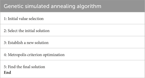
Table 1. Schematic diagram of simulated annealing algorithm with genetic algorithm.

2.5 Metropolis criterion optimization

The Metropolis criterion is an optimization strategy based on stochastic simulation which was first proposed by Nicholas Metropolis and colleagues; it has been widely used in the field of scientific computing after being promoted and improved by subsequent research. The central concept revolves around utilizing a probabilistic model to mimic the behavior of the objective function, with the goal of identifying either the global or local optimal solution (Kezhen et al., 2024). Specifically, the Metropolis criterion determines the acceptance of a new solution by defining an energy (or objective) function, randomly generating the new solution, and calculating the transition probability based on the energy difference between the new and the current solution using the probability distribution function. This method is especially suitable for dealing with high-dimensional, nonlinear, and complex optimization problems, and the algorithm has convergence guarantee (Golpira et al., 2016). The process of enhancing the simulated annealing algorithm involves the following steps. Figure 2 illustrates the fundamental operation flow chart for improving the simulated annealing algorithm. The operations highlighted in darker shades in the flow chart incorporate elements from genetic algorithms.

(1) Initialization control parameters: population size $chrom\_Hz$, Markov chain length $L$, selection probability $px$, crossover probability $pc$, mutation probability $\mathit{pr}$, initial temperature $T_0$, cooling coefficient $q$, and termination temperature $T_e$.

(2) In the initial solution construction, the idea of genetic algorithm coding and generating the initial population is combined with random initialization of $chrom\_H\mathrm{z}$ frequency, and the initial population $chrom$ is generated. The value of the objective function is computed for each datum within the initial population $chrom$. The chromosome corresponding to the smallest objective function value is selected as the initial solution $Z_0$, which is also the current optimal solution, and the objective function value $Z_{best}=Z_0$ is calculated.

(3) Set the number of iterations of the current temperature to $u=0$.

(4) The process of generating novel solutions shifts from random creation to a sequence of selection, crossover, and mutation operations. These operations are applied to the population in order to yield a fresh solution. Selection identifies promising individuals, crossover combines their genetic material, and mutation introduces variation, collectively contributing to the evolution of new, potentially improved solutions.

(5) Calculate and determine increment $\Delta f=f\left(Z_1\right)-f\left(Z_0\right)$.

(6) Judgment $\Delta f$: if $\Delta f<0$, then $Z_1$ is accepted as the new current solution, i.e., $Z_{best}=Z_0$; if $\Delta f\ge 0$, the acceptance probability of $Z_1$ is calculated, and a random number $p=\exp \left(-\Delta f/T\right)$ evenly distributed over the interval [0,1] is generated. At this time, $h=random\left[0,1\right]$ is embraced as the updated current solution; otherwise, the current solution $Z_0$ is retained.

(7) Determine whether the algorithm meets the conditions for ending the current temperature iteration. If $u<L,u=u+1$, perform Step 4; if $u>L$, go to Step 8.

(8) Determine whether the algorithm reaches the end temperature $T_e$; if $current\text{\hspace{0.17em}temperature}T\le \text{final\hspace{0.17em}temperature}{T}_e$, output the optimal solution, end the algorithm; if $T>T_e,T=T\times q$ cooling, perform Step 3.

Figure 2

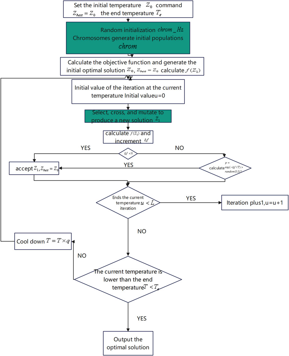
Figure 2. Flow chart of improved simulated annealing algorithm.

3 Application

As shown in Figure 3 the simulation model of the IEEE-14 node system is constructed using Matlab/Simulink and the PSASP platform, with the inclusion of a wind farm at node 1 and a photovoltaic power plant at node 3. The efficiency of the photovoltaic system is not constant but is deeply influenced by environmental factors, especially the intensity of solar radiation and the temperature of photovoltaic cells. Wind power generation is affected by many factors, such as climate and geographical location. The power it emits fluctuates greatly, and the quality is uneven. The characteristics of every individual component and the recently installed wind turbine can be found in Tables 2 and 3.

Figure 3

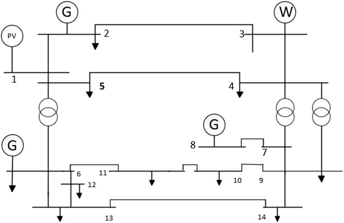
Figure 3. Topology of IEEE-14 nodes.

Table 2

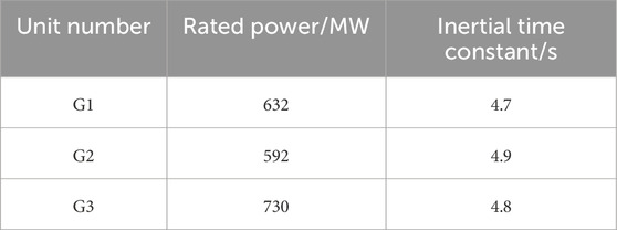
Table 2. Parameters of the synchronous generator set.

Table 3

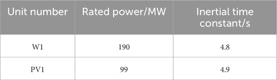
Table 3. Parameters of the new energy generator set.

3.1 System frequency response curve

The system PSASP simulation model experiences a disturbance of $\Delta P_{\mathrm{d}}=0.03p.u.$ at the $t_0$ node. The precision of the system’s frequency response model is evaluated by observing the alterations in the frequency fluctuations of $\Delta f$ within the model. Observing the graph in Figure 4, it is evident that following the inertia response and comprehensive tuning of the primary frequency regulation system, the system frequency gradually converges toward a stable state, surpassing the point of maximum frequency deviation. At t = 9.67241 s, the system reaches the maximum frequency deviation point and the maximum system frequency deviation is $\Delta f_{\max }=$ 0.0688 Hz.

Figure 4

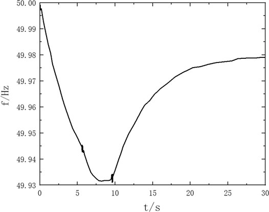
Figure 4. Frequency change curve of the power system.

3.2 System minimum inertia requirement verification

Considering the maximum frequency deviation and the maximum RoCoF, the minimum inertia calculation of a new power system should consider the maximum value under two constraints:

$H_{\min }=\max \left\{H_{RocoF},H_{\text{Frequency}\text{deviation}}\right\}.(17)$

According to Formula 17, the system inertia range is calculated according to the maximum deviation of frequency and the range value of RoCoF, and the maximum value of both is taken as the minimum inertia of the system. In this section, the IEEE-14 node system (Figure 4) is used for simulation; the changes in air volume caused by power fluctuation and load power increase are two cases of verification.

First, power disturbance is applied to the system, and the required RoCoF and frequency change are given to evaluate the inertia required by the system. The actual system inertia is then compared, and the actual frequency change rate and frequency change are compared with the given to observe whether the simulation results are consistent with the theory.

3.2.1 Wind power fluctuation causes unbalanced power of 30 MW

At 43S, the wind power is set to fluctuate suddenly, and the unbalanced power of the system caused by the fluctuation is 30 MW. Figure 6 shows the RoCoF of the faulty node and the frequency fluctuation after the disturbance.

It can be seen from Figure 5 that the maximum frequency offset is 0.18 Hz and RoCoF is 0.154 Hz/s. Assuming that $\Delta f=0.16Hz$, it is calculated that the required inertia of the system is 4332 MW·s. Assuming RoCoF = 0.16 Hz/s, the required inertia of the system is 3120 MW·s, while the actual inertia of the system is only 3065 MW·s. The actual inertia is lower than the required inertia, and the RoCoF and frequency deviation in the simulation results are greater than the assumed values. The results agree with the theory.

Figure 5

Figure 5. Parameter changes after wind power fluctuation of 30 MW.

3.2.2 Penetration rate of wind power is 10%, and unbalanced power caused by load increase is 30 MW

At this time, the wind power penetration rate of the system is 20%. At 45 s, the unbalanced power of the system caused by the increase of load power is 35 MW. Figure 8 shows the RoCoF and frequency fluctuation of the faulty node after the disturbance.

As can be seen from Figure 6, the maximum frequency offset is 0.46 Hz, and RoCoF is 0.26 Hz/s. Assuming $\Delta f=0.4Hz$, the required inertia of the system is 2670 MW·s through calculation, and RoCoF = 0.2 Hz/s. The required inertia of the system is 2475 MW·s, while the actual inertia of the system is only 2865 MW·s. The actual inertia is higher than the demand inertia, and the results agree with the theory.

Figure 6

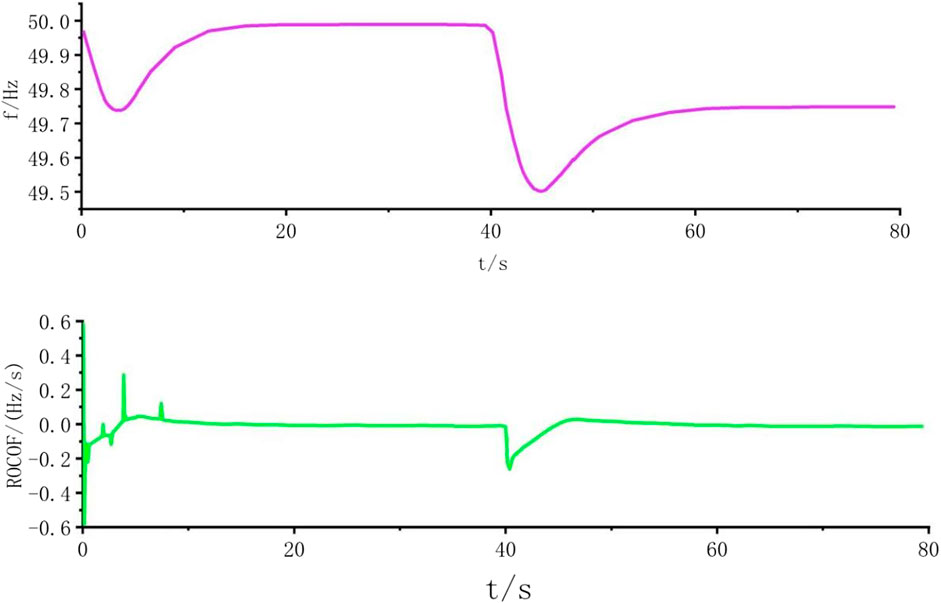
Figure 6. Load increase causes power fluctuation after RoCoF and $f$.

In the above experiments, we performed multiple groups of different control experiments under the same working conditions, and the accuracy of the inertia evaluation calculation method used in this paper was more than 99%. In the frequency adjustment of the power system, the inertia response time was in the millisecond range, the solution speed of the inertia estimation was optimized, and the experimental level reached the millisecond level.

3.3 Evaluation of minimum inertia of a system

Based on the simulation model, an active power disturbance $\Delta P_d=0.04p.u$ is applied to the load node five at time $t=0s$. According to the constraint conditions of Formulas 3–5, each initial value is brought into the improved simulated annealing algorithm to solve, in which the maximum frequency deviation is at an interval of 0.02 Hz, RoCoF is at an interval of 0.05 Hz/s, the simulation solution step is 0.02 s, and the algorithm solution time is 30 s.

As can be seen from Figures 7, 8, the RoCoF constraint of the system frequency change rate and the maximum deviation $\Delta f$ constraint of the system frequency are negatively correlated with the minimum inertia of the system. Specifically, the smaller the constraint conditions $RoCo{F}_{\max }$ and $\Delta f_{\max }$, the greater the demand for the minimum inertia of the system. In addition, compared with the power system without virtual inertia of new energy, the power system that includes virtual inertia of new energy has better frequency response due to its additional inertial support capability of new energy, and the system has less demand for inertia under the same constraint conditions.

Figure 7

Figure 7. Inclusion of minimum inertia demand assessment of the new energy virtual inertia system.

Figure 8

Figure 8. Exclusion of minimum inertia requirement assessment of the new energy virtual inertia system.

Taking system $RoCo{F}_{\max }=0.4Hz/s,\Delta f_{\max }=0.15Hz$ as an example, the minimum inertia required for two different systems is shown in Tables 4, 5.

Table 4

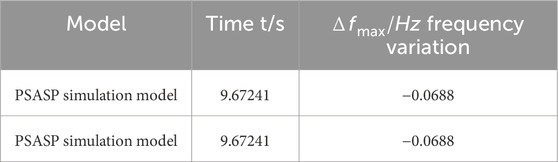
Table 4. Maximum points of system frequency variation.

Table 5

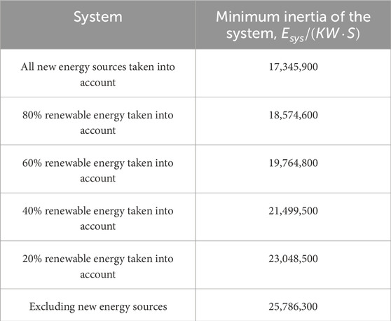
Table 5. Minimum inertia requirement of the system with different percentages of new energy output.

Current analysis techniques consider both the RoCoF and frequency deviations, constructing a minimum inertia requirement assessment model aimed at preserving frequency stability in both islanded and grid-connected operation modes. Both the existing methods and the present study share a foundation in frequency constraints to derive the system’s minimum inertia threshold. However, this study goes beyond the mere constraint by incorporating the processing limitations of generator sets, thereby aligning more closely with real-world production environments and amplifying the impact factors of virtual inertia on the generator side. Table 6 provides further details on these aspects.

Table 6

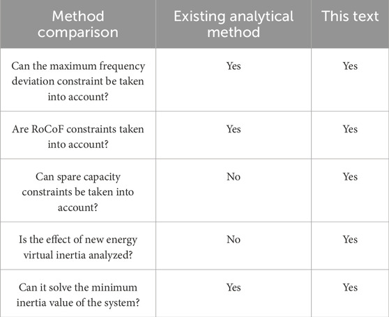
Table 6. Comparison of existing analytical methods with the analytical methods in this paper.

4 Conclusion

This study establishes a framework for assessing minimal inertia within an electrical power system encompassing the virtual inertia derived from renewable energy sources. A methodology for evaluating the minimal inertia of such a system, inclusive of the virtual inertia component from new energy technologies is also introduced. The evaluation of frequency response in power systems, incorporating the virtual inertia effect of new energy, is accomplished. The accuracy of this presented approach is confirmed through simulations based on the IEEE-14 bus model. The key findings are summarized below.

(1) The investigation underscores the pivotal significance of the terminal inertia response phase in the frequency response of a power system for ensuring grid frequency security. Specifically, the magnitude of inertia directly correlates with the maximum deviation in power system frequency and the system’s resilience against disturbances. The frequency response model constructed in this paper yields a maximum frequency offset of 0.0688 Hz.

(2) The improved simulated annealing algorithm innovatively proposed in this paper considers whether the genetic algorithm on the traditional simulated annealing algorithm can ignore the effect of the cooling rate parameter on the simulated annealing algorithm. The minimum inertia of the solved system ranges from 25,786,300 KW-S from the non-new energy unit to 17,345,900 KW-S from 100% new energy unit in the system.

(3) Using a simulated annealing algorithm to solve the minimum inertia of the system can significantly improve the stability and dynamic response capability of the high percentage of new energy grid, providing key technical support for the safe and efficient operation of a future low-carbon energy system; its global optimization characteristics can also promote the development of multi-timescale inertia resource cooperative control strategy, help build a more resilient and adaptive new power system, and accelerate the energy green transition process.

Data availability statement

The raw data supporting the conclusions of this article will be made available by the authors, without undue reservation.

Author contributions

QZ: data curation, writing – original draft, and writing – review and editing. QJ: methodology, writing – original draft, and writing – review and editing. TZ: project administration, validation, writing – original draft, and writing – review and editing. HZ: Supervision, Project administration, writing – original draft. CW: methodology, writing – original draft, and writing – review and editing. WL: conceptualization, writing – original draft, and writing – review and editing.

Funding

The author(s) declare that financial support was received for the research and/or publication of this article. This project was supported by Technology Projects of State Grid (2023YF-76).

Conflict of interest

QZ, JQ, TZ, HZ, CW, and WL were employed by State Grid Liaoning Electric Power Academy.

Generative AI statement

The authors declare that no generative AI was used in the creation of this manuscript.

Publisher’s note

All claims expressed in this article are solely those of the authors and do not necessarily represent those of their affiliated organizations, or those of the publisher, the editors and the reviewers. Any product that may be evaluated in this article, or claim that may be made by its manufacturer, is not guaranteed or endorsed by the publisher.

References

Bo, W., Deyou, Y., and Guowei, C. (2020). Research review on inertia related problems of power system under high proportion new energy access. Power Syst. Technol. 44 (08), 2998–3007.

Google Scholar

Fu, S., Sirui, L., Guodan, O., Shan, J., Cao, Y., Wang, Z., et al. (2023). Inertia estimation of power system with new energy considering with high renewable penetrations. Energy Rep. 9 (S7), 1066–1076. doi:10.1016/J.EGYR.2023.04.147

CrossRef Full Text | Google Scholar

Golpira, H., Seifi, , Messina, A. R., and Haghifam, M. R. (2016). Maximum penetration level of micro-grids in large-scale power systems: frequency stability viewpoint. IEEE Trans. Power Syst. A Publ. Power Eng. Soc. 31 (6), 5163–5171. doi:10.1109/tpwrs.2016.2538083

CrossRef Full Text | Google Scholar

Huadong, S., Bing, Z., Shiwen, X., Lin, Y., Baocai, W., Wenfeng, L., et al. (2024). Definition, classification and analysis methods of strength of high scale power electronic power systems. Chin. J. Electr. Eng. 44 (18), 7039–7049. doi:10.13334/j.0258-8013.pcsee.231299

CrossRef Full Text | Google Scholar

Jiebei, Z., Heyu, L., Lujie, Y., Sichang, Y., Liyuan, G., Zhao, L., et al. (2024). Prospect of new power system inertia-frequency “cloud-network-end” sensing and control technology. High Voltage Technology 50 (07), 3090–3104. doi:10.13336/j.1003-6520.hve.20240200

CrossRef Full Text | Google Scholar

Kezhen, L., Huaping, T., Chunhao, Y., Peng, L., Yanxia, C., Wei, P., et al. (2024). A regional inertia estimation method for power systems considering system partitioning and node frequency dynamic response. Power Automation Devices 49, 1–17. doi:10.16081/j.epae.202412005

CrossRef Full Text | Google Scholar

Lin, X., Wen, Y., and Yang, W. (2021). Inertial safety domain: concept, characteristics and evaluation methods. Proc. Chin. Soc. Electr. Eng. (09), 3065–3079.

Google Scholar

Mercier, P., Cherkaoui, R., and Oudalov, A. (2009). Optimizing a battery energy storage system for frequency control application in an isolated power system. IEEE Trans. Power Syst. 24 (3), 1469–1477. doi:10.1109/TPWRS.2009.2022997

CrossRef Full Text | Google Scholar

Patricia, D. M., Adolfo, A., Javier, R., Prodanović, M., and García-Cerrada, A. (2024). Coordination of distributed resources for frequency support provision in microgrids. Int. J. Electr. Power Energy Syst. 155 (PB), 109539. doi:10.1016/J.IJEPES.2023.109539

CrossRef Full Text | Google Scholar

Pratap, C. N., Sonalika, M., Ramesh, C. P., and Sidhartha, P. (2023). Hybrid whale optimization algorithm with simulated annealing for load frequency controller design of hybrid power system. Soft Comput. doi:10.1007/s00500-023-09072-1

CrossRef Full Text | Google Scholar

Ruyin, S., Lei, X., Liang, Q., Junjie, Z., Ruiqi, L., and Kaipei, L. (2025). Advances in Minimum Inertia Demand Assessment for Novel Power Systems. Beijing: Tongfang Knowledge Network Technology Co., Ltd. 1–13. doi:10.13336/j.1003-6520.hve.20250192

CrossRef Full Text | Google Scholar

Shetty, P. N., and Chakrasali, R. (2021). Intentional/un-intentional islanding control strategy for distributed generation system. Int. J. Adv. Intell. Paradigms 19 (2), 146–160. doi:10.1504/IJAIP.2021.115246

CrossRef Full Text | Google Scholar

Shichun, L., Mengen, L., Jiachang, L., Mingda, S., Tiao, Y., and Zhenxing, L. (2025). Deep mining inertia auxiliary service strategy for virtual inertia compensation in wind power. J. Power Syst. Autom., 1–9. doi:10.19635/j.cnki.csu-epsa.001572

CrossRef Full Text | Google Scholar

Song, J., Zhou, X., Zhou, Z., Wang, Y., Wang, Y., and Wang, X. (2023). Review of low inertia in power systems caused by high proportion of renewable energy grid integration. Energies 16, 6042. doi:10.3390/EN16166042

CrossRef Full Text | Google Scholar

Xia, D., Wei, S., and Xiao, H. (2018). Integrated control method of energy storage battery participating in primary frequency modulation. High. Volt. Tech. 44 (4), 1157–1165.

Google Scholar

Yefeng, J., Yuxiang, X., Lin, S., Chen, F., Jianguo, Y., and Qi, W. (2024). An inertia configuration method based on frequency space characteristics and sensitivity analysis. Power Automation Devices. 1–13. doi:10.16081/j.epae.202412019

CrossRef Full Text | Google Scholar

Yunfeng, W., and Huangxiao, L. (2021). Evaluation of the minimum inertia requirement of microgrids in islanding and grid-connected modes. Proc. CSEE 41 (06), 2040–2053. doi:10.13334/j.0258-8013.pcsee.200899

CrossRef Full Text | Google Scholar

Zhang, J., Zhang, S., and Niu, Y. (2019). A high proportion of new energy access-combined cooling, heating, and power system planning method. Int. J. Energy Res. 43 (14), er.4755–7955. doi:10.1002/er.4755

CrossRef Full Text | Google Scholar

Zhang, W. Q., Wen, Y. F., and Chi, F. D. (2021). Research framework and prospect of inertia evaluation of power system. Proc. CSEE 41, 6842–6856.

Google Scholar

Zhenhao, W., Shilun, C., JInming, G., Guoqing, L., Chaobin, W., and Guangzhi, L. (2023). A minimum inertia assessment method for power systems taking into account the frequency regulation capability of new energy field stations. Journal of Solar Energy 45 (08), 494–502. doi:10.19912/j.0254-0096.tynxb.2023-0540

CrossRef Full Text | Google Scholar

Zhiyong, H., Zhibo, H., Bo, W., Yanping, W., Lei, S., and Xiangzhen, Y. (2025). A coordinated optimisation strategy for virtual inertia of energy storage plant considering the effect of multiple dead zones. Energy Storage Science and Technology, 1–13. doi:10.19799/j.cnki.2095-4239.2024.1187

CrossRef Full Text | Google Scholar

Zimin, Z., Yu, D., Xiaoyun, W., Wu, G., and Ma, J. (2023). Analysis of minimum rotational inertia requirements for power system frequency stability. J. Phys. Conf. Ser. 2661 (1), 012007. doi:10.1088/1742-6596/2661/1/012007

CrossRef Full Text | Google Scholar