Collaborative optimal operation control of HVAC systems based on multi-agent

The HVAC system of public buildings, as a thermostatically controlled load, accounting for a relatively significant proportion of building energy consumption. Therefore, it is necessary to optimize energy efficient of HVAC systems in public buildings. Nevertheless, the complication of HVAC systems is on the rise. As a consequence, the computing efficiency of optimization algorithms is relatively low, posing challenges for real-time optimal operation control. Hence, there is an immediate requirement to boost both the energy efficiency of the system and the computing efficiency in order to strengthen the system’s robustness. In this paper, a collaborative optimization approach based on multi-agent is initially put forward to address the overall optimization issue (OOI) of a complicated HVAC system. The OOI is disintegrated into numerous sub-optimization issues within the multi-agent structure. These sub-issues take into account the interaction features among components. By doing so, the complication of the OOI within HVAC systems is effectively decreased. Secondly, the adaptive hybrid-artificial fish swarm algorithm (AH-AFSA) is proposed for solving optimization issues with mixed decision variables. Finally, the effectiveness of the proposed method is verified by an arithmetic example. The analysis reveals that the proposed approach is capable of reducing power consumption by 18.9% and the computation time for each operation condition is 12.2 s, which saves about 54% of time cost compared with the centralized method, and can enhance the computing efficiency of the optimization approach for a complicated HVAC system while reducing power consumption.

1 Introduction

Heating, ventilation and air conditioning (HVAC) system, as a thermostatically controlled load, plays a crucial role in regulating the indoor thermal environment of public buildings, which consists of a number of electromechanical devices with nonlinear characteristics (Cao and Ren, 2018; Li et al., 2018; Cheng, 2019). Typically, HVAC systems are designed to handle the maximum cooling load of public buildings, which accounts for more than 50% of the total energy consumption of the building (Zhuang et al., 2023). Therefore, there is substantial potential for energy conservation during part - load operation in HVAC systems. Nevertheless, because of the inherent characteristics of nonlinearity and coupling in HVAC systems, the pursuit of optimal energy efficiency in actual operation encounters substantial difficulties.

Optimizing the operation of an HVAC system requires consideration of the interactions between multiple components of the HVAC system due to their strong nonlinearities and coupling properties. Typically, OOI within HVAC systems involve the optimization of switching sequence of homogeneous components, which called allocational problems (AP) and control loop set magnitudes, which called diffusional problems, DP). The optimization of AP belongs to the category of 0–1 integer programming problems, which the decision variable is discrete. In contrast, the optimization of DP entails the decision variable that are continuous. Therefore, the OOI of HVAC systems fall into the category of mixed optimization problems. In order to substantially improve the overall operating performance of an HVAC system that includes homogeneous components, it is necessary to resolve both the AP and the DP during the optimization.

In recent years, there has been an increasing emphasis on improving the energy efficiency of HVAC systems through the use of intelligent techniques such as Genetic Algorithms (GA) (Xiong and Wang, 2020), Artificial Neural Networks (ANNs) (Jang et al., 2021), Particle Swarm Optimization (PSO) (Afroz et al., 2022), etc. HVAC systems configured to contain identical paralleled units of varying capacities can better adapt to changes in the cooling demand under part-load conditions by employing differential evolutionary methods (Lee et al., 2011) to solve the energy optimization problem of chiller units under low cooling demand conditions and improve the energy efficiency of the HVAC system with parallel CH. An improved sparrow search algorithm (Li et al., 2023) was used to improve the energy saving potential of the HVAC system, in addition, intelligent algorithms such as enhanced artificial fish swarm algorithm (Zheng et al., 2019), cuckoo search algorithm (Coelho et al., 2014) and invasive weed optimization algorithm (Zheng and Li, 2018) were used to solve the energy optimization among the same type of parallel components of the HVAC system. To further enhance the versatility of practical HVAC control systems, distributed control frameworks have been developed with improved AFSA algorithms in order to optimize the flow rate distribution problem for parallel pumps (Yu et al., 2018). In addition, a multi-agent based distributed approach (Li and Wang, 2020) is used to solve the airflow distribution problem in ventilation systems, which provides a reference for the subsequent use of intelligent distributed algorithms to optimize airflow distribution in multi-zone HVAC systems (Salsbury et al., 2023).

However, the aforementioned studies have focused on parallel components or subsystems of the same type in an HVAC system (the allocation problem), while neglecting the interactions between components or subsystems (the diffusion problem). Since the HVAC system is intricate system made up of diverse components having nonlinear traits, considering the interactions among components is crucial for better optimization and control. The Firefly Algorithm (FA) (Coelho and Mariani, 2013), the Artificial Bee Colony Algorithm (Zhang et al., 2013), and the Differential BAT Algorithm (DBA) (Dos Santos Coelho and Askarzadeh, 2016) have been shown to be effective in solving the problem of solving the diffusion optimization problem and improving the energy efficiency of the components of an HVAC system. The aforementioned studies emphasize the effectiveness of heuristic search algorithms such as genetic algorithm (GA), differential evolution (DE), and particle swarm optimization (PSO), in dealing with the nonlinear properties of HVAC systems, which can bring about remarkable energy conservation. In addition, the introduction of integrated back-propagation neural networks and Gray Wolf Optimizer (GWO) methods (Li et al., 2021) in adjacent components of HVAC can optimize the control effectiveness and energy efficiency of adjacent components of HVAC systems. Similarly, the potential to reduce the energy consumption of the HVAC system by 15.3% was successfully achieved by using an online optimization approach based on a simplified heat transfer model cooling water system (Ma, 2021).

However, most of the studies mentioned above have only concentrated on solving either the AP or the DP, failing to achieve an overall balance. From the perspective of global optimization, research on addressing mixed optimization problems is scarce. In general, homogeneous components of different capacities are installed in HVAC systems so that they can better respond to the fluctuation in cooling demand during part - load situations. However, existing studies are usually unable to take into account the suitability and practicality of the proposed optimization approach to solve the OOI for such the complicated system. Although some studies aim to improve computing efficiency, usually concentrate on the components of subsystems, ignoring the necessity of balancing trade - offs between components, thus rendering these approaches inappropriate for overall optimization. Hence, it is immediately required to find an excellent optimization methodology for the purpose of simplifying mixed optimization problems, alleviating the computing burden and keeping the HVAC system’s energy efficiency.

Recent advancements in multi-agent frameworks have offered promising solutions to these challenges. Distributed reinforcement learning (DRL) enables agents to learn adaptive control policies through real-time interactions with dynamic environments, while heterogeneous agent collaboration models effectively balance trade-offs between discrete and continuous decision spaces. For instance, multi-agent deep Q-network (MADQN) has reduced HVAC energy consumption by 15% by coordinating chiller start-stop sequences and airflow control. Similarly, federated learning architectures have enhanced privacy-preserving optimization in multi-zone HVAC systems. Despite these innovations, existing studies rarely integrate configuration optimization (AP) and operational optimization (DP) within a unified framework, limiting their applicability to complex HVAC systems with mixed optimization requirements.

Looking deeper, distributed optimization and multi-agent networks complement each other, with multi-agent networks serving as the concrete carrier of distributed optimization algorithms (Majzoobi et al., 2018). Each agent, as an autonomous entity with sensing, communication, computing, and execution capabilities, forms a large-scale network system through local collaboration. Compared with centralized control, distributed control not only significantly reduces problem complexity and scale by decomposing complex large-scale systems into multiple subsystems but also remarkably improves work efficiency (Labeodan et al., 2015). Meanwhile, its advantages of good scalability, high reliability, and ease of maintenance have been widely recognized (Kim et al., 2019). Wang et al. developed a multi-agent control system (Wang et al., 2012) that takes indoor comfort and energy consumption as objective functions to achieve comprehensive optimization of indoor temperature, lighting, and indoor air quality (IAQ). Yang et al. developed a user-centered multi-agent control system (Yang and Wang, 2013) to optimize energy utilization efficiency and IAQ in ventilation systems. Cai et al. established a general multi-agent control system (Cai et al., 2015; 2016) that provides optimization algorithms for energy and air conditioning systems. Michailidis et al. proposed a novel decentralized agent-based model-free optimal control method (Michailidis et al., 2018) for modern non-residential buildings to enhance energy performance. These studies have laid a solid foundation for the application of multi-agent frameworks in HVAC systems and pointed out directions for follow-up research.

To address these gaps and improve the energy efficiency and computational efficiency of complex HVAC systems, this paper proposes a collaborative optimal operation control method based on multi-agent of HVAC systems that combines the superiority of heuristic algorithms. A number of simpler subproblems are derived from complicated mixed optimization problems. Different agents are assigned to deal with each subproblem, with the interactions among components being taken into consideration. For the purpose of ensuring that agents cooperate concurrently to acquire the most suitable switching sequence and set magnitudes, an AH-AFSA is introduced in this paper to deal with the OOI.

2 HVAC system model

Figure 1 illustrates a framework for synergistic operation optimization of HVAC systems, which major consist of chilled water pumps (CHWP), chiller plants (CH), air handling units (AHU), cooling towers (CT) and cooling water pumps (CWP). However, the inherent nonlinear nature of these components of an HVAC system results in energy efficiency tradeoffs among components. AP and DP are two common types of tradeoff issues that often occur in the variable flow HVAC system of public buildings. DP occur principally between neighboring components such as chillers, pumps, and fans, which are used to characterize the energy-efficiency tradeoffs between them. AP occur primarily between homogeneous components with different capacities.

Figure 1

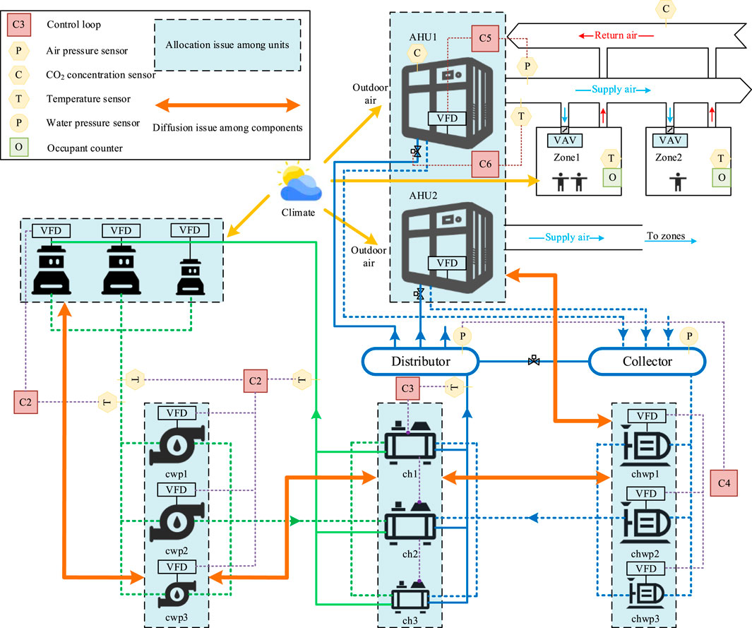
Figure 1. Collaborative operation optimization framework of HVAC system.

Therefore, this paper aims to consider the energy efficiency trade-offs between different components in an HVAC system as well as between neighboring components with different capacities, and how to assign the corresponding weights in order to coordinate the resources within HVAC systems to minimize the energy consumption of HVAC systems’ synergistic operation, which in turn reduces the user’s cost. The decisions related to the HVAC system in this paper are as follows.

(1) The output of the different components in the HVAC system $P_{sys}$;

(2) The outputs of different capacities of the same component in the HVAC system are $P_{ch}$, $P_{chwp}$, $P_{cwp}$, $P_{ct}$ and $P_{ahu}$ respectively.

2.1 HVAC system component characterization model

At the beginning of section 2.1, coupling characteristic and the components of HVAC systems will be systematically modeled. Usually, homogeneous operation components are categorized according to the number into 0/1 discrete or integral types, which are expressed by $N_{i,mix}$ and $N_{d,mix}$, expressed by Equation 1.

$N_{d,mix}=\left\{N_{d,mix,1},\cdots ,N_{d,mix,l},\cdots ,N_{d,mix,N_{mix}}\right\},mix\in \left\{cwp,chwp,ct,ahu,ch\right\}(1)$

$N_{i,mix}={\sum }_{l=1}^{N_{mix}}{N}_{d,mix,l}(2)$

where the relationship with $N_{i,mix}$ and $N_{d,mix}$ can be expressed by Equation 2. Using $N_{d,mix,l}$ to denote the switching condition, which is discrete binary variable. $N_{mix}$ indicates the overall quantity of units, mix indicates component types, and l indicates the lth unit of components.

2.1.1 Chiller model

The Stoecker model, which is presented in Equations 3–5, can be used as a reference for the parallel CH model.

$P_{ch}={\sum }_{h=1}^{N_{ch}}\left(P_{CH,ch,h}·f_{PLR,ch,h}·f_{T,ch,h}·N_{d,ch,h}\right)(3)$

$f_{PLR,ch,h}=a_{0,h}+a_{1,h}\left(\frac{Q_{ch,h}}{Q_{ch,R,h}}\right)+a_{2,h}{\left(\frac{Q_{ch,h}}{Q_{ch,R,h}}\right)}^2(4)$

$f_{T,ch,h}=b_{0,h}+b_{1,h}{T}_{E,o}+b_{2,h}{T}_{E,o^2}+b_{3,h}{T}_{C,o}+b_{4,h}{T}_{C,o^2}+b_{5,h}{T}_{E,o}{T}_{C,o}(5)$

where the subscript R denotes the rated value, $f_{PLR,ch,h}$ and $f_{T,ch,h}$ represent the correction factors. The meaning of subscripts C and E respectively signify the condenser and evaporator, and coefficients a₀∼a₂ and b₀∼b₅ can be determined by fitting the sample data. Subscript o denotes the value of the outlet parameter.

2.1.2 Chilled water pump model

According to both fans and pumps characteristics, the CHWP model can be described by Equation 6.

$P_{chwp}={\sum }_{u=1}^{N_{chwp}}\left(\frac{m_{chw,u}·H_{chw,u}}{g_c·{\eta }_{chw,u}}{N}_{d,chwp,u}\right)(6)$

where $g_c$ represents the constants associated with H and m, $m_{chw}$ means pump flow, $H_{chw}$ means head. Supposing the gravitational acceleration to be 9.8 m/s², and the units of H and m are respectively mH₂O and m³/h, $g_c$ is equal to 367.3. In addition, if H is in kPa and m is in kg/s, $g_c$ turns into 134.9. $\eta$ represents the pumps and fans efficiencies linked to H and m, which derived from data fitting.

2.1.3 Cooling water pump model

Since the cooling water circuit is of an open system nature, the parallel CWP model, as shown in Equation 7, diverges from the CHWP model.

$\begin{array}{ll}\hfill P_{cwp}& ={\sum }_{m=1}^{N_{cwp}}{P}_{cwp,R,m}{N}_{d,cwp,m}\left[c_{0,m}+c_{1,m}PL{R}_{cwp,m}+c_{2,m}{\left(PL{R}_{cwp,m}\right)}^2\right.\hfill \\ \hfill & \left.+c_{3,m}{\left(PL{R}_{cwp,m}\right)}^3\right]\hfill \end{array}(7)$

where coefficients c₀∼c₃ are determined by data fitting, $PL{R}_{cwp,m}$ is the partial load rate of the mth cooling water pump, defined as the ratio of the actual flow rate to the rated flow rate (Wang and Zhao, 2024), as follow Equation 8.

$PL{R}_{cwp,m}=\frac{m_{cw,m}}{m_{cw,R,m}}(8)$

2.1.4 Cooling tower model

The CT model is represented in Equation 9.

$P_{ct}={\sum }_{n=1}^{N_{ct}}{P}_{ct,R,n}{N}_{d,ct,n}\left[d_{0,n}+d_{1,n}PL{R}_{ct,n}+d_{2,n}{\left(PL{R}_{ct,n}\right)}^2+d_{3,n}{\left(PL{R}_{ct,n}\right)}^3\right](9)$

where $PL{R}_{ct,n}$ is the partial load rate of the fan (Seong et al., 2019), which can be calculated as follow Equation 10. The coefficients d₀∼d₃ can be determined by data fitting.

$PL{R}_{ct,n}=\frac{m_{a,n}}{m_{a,R,n}}(10)$

2.1.5 Air handling unit model

For the AHU model, the airflow of the kth AHU can be calculated from the airflow of each air-conditioned room as follow Equation 12. Equation 13 can be used to simply express the heat exchange between the air side and the water side of coils. Therefore, the AHU model is shown in Equation 11.

$P_{ahu}={\sum }_{k=1}^{N_{ahu}}\frac{m_{sa,k}{H}_{sa,k}}{g_c·{\eta }_{ahu,k}}(11)$

$m_{sa,k}={\sum }_{b=1}^{N_{room}}{m}_{sa,k,b}(12)$

${\sum }_{b=1}^{N_{room}}{Q}_{k,b}=\frac{e_{1,k}·m_{sa,k}^{e_{3,k}}\left(T_{ma,k}-T_{E,o}\right)}{1+e_{2,k}·{\left(m_{sa,k}/m_{chw,k}\right)}^{e_{3,k}}}(13)$

where, $T_{ma}$ denotes the mixed air’s temperature, $m_{sa}$ indicates the flow rate of the coil water within the AHU, coefficients e₁∼e₃ are model coefficients determined by data fitting. Similar to the coil model, the heat exchange between the air side and the water side of the cooling tower (Zhao et al., 2021) can be expressed as follow Equation 14:

$P_{ch}+{\sum }_{i=1}^{N_{ch}}{Q}_{ch,i}={\sum }_{n=1}^{N_{ct}}\left(\frac{g_{1,n}·m_{cw,n}^{g_{3,n}}\left(T_{C,i}-T_{wb,od}\right)}{1+g_{2,n}·{\left(m_{cw,n}/m_{a,n}\right)}^{g_{3,n}}}\right)(14)$

where, $T_{wb,od}$ is the outdoor wet bulb temperature, $m_{cw}$ is the cooling tower water flow rate, $m_a$ is the cooling tower airflow, and g₁∼g₃ are the model coefficients, which can be obtained by data fitting.

2.2 HVAC system model constraints

From the model in Section 2.1, it is clear that the power consumption of each component depends solely on its operational parameters, e.g., $P_{ch}$, it is only affected by $Q_{ch}$, $T_{E,o}$, $T_{C,o}$, and $P_{ct}$ is only related to $m_a$, etc. However, in practical systems, an interaction exists among the operational parameters of distinct components, resulting in the problem of the compromise in energy efficiency among components. In a set magnitudes problem with control loops (DP), constraints of the DP are represented in Equation 15.

$L_{\mathit{min}}\le X^{*}\le L_{\mathit{max}},X\in \left\{T_{E,o},H_{chwp},\Delta T_C,T_{C,i},T_{sa},H_{sa}\right\}(15)$

where L denotes the set of boundaries. In the switching ordering of homogeneous components (AP), the decision variables must satisfy the basic system requirements: there must be at least one operating unit of each component type. Therefore, the constraints of the AP are defined as follow Equation 16. In addition, constraints on the upper and lower limits of the allocation quantity are represented in Equation 17.

$N_{d,mix}\ne \left\{0\right\}(16)$

$s_{mix,\mathit{min}}\le s_{comp}\le s_{mix,\mathit{max}},s_{mix}\in \left\{Q_{ch},m_{chw},m_{cw},m_a,m_{sa}\right\}(17)$

In order to facilitate the use of intelligent algorithms to find the optimal solution, the above constrained optimization problem needs to be transformed into an unconstrained optimization problem. Constraints in Equations 15, 16 belong to decision variables, which can be constrained to the feasible solution space of the algorithm. For the constraint in Equation 17, the allocation optimization problem can be transformed into an unconstrained problem by constructing a penalty function (Seo, 2014; Wang, 2024).

To effectively solve the above-mentioned constrained nonlinear optimization problem, a penalty function is typically designed and incorporated into the original optimization problem. This helps transform the constrained optimization problem into an unconstrained one. In this study, the optimization parameter constraints described by inequalities (15) and (16) can be directly integrated into the solution space of the optimization algorithm without resorting to penalty functions. However, the operational condition constraints specified in the inequalities (17) will be converted into unconstrained problems by constructing penalty functions.

Therefore, the constrained optimization problem specified in Equation 18 can be transformed into the unconstrained optimization problem expressed in Equation 19. Here, $P_i\left(x_i\right)$ represents the penalty function, as shown in Equation 20; $J_i$ denotes the penalty coefficient, which should be set to a relatively large positive number.

$\min f\left(X\right),\mathrm{s}.\mathrm{t}.s_{i,mix,\mathit{min}}\le s_{i,comp}\left(x_i\right)\le s_{i,mix,\mathit{max}}(18)$

$\min F\left(X\right)=\min \left[f\left(X\right)+{\displaystyle \sum _{i=1}^p}{P}_i\left(x_i\right)\right](19)$

$\left)=\left\{\begin{array}{ll}0,& s_{i,mix,\min }\le s_{i,comp}\left(x_i\right)\le s_{i,mix,\max }\\ J_i{\left[s_{i,comp}\left(x_i\right)-s_{i,mix,\min }\right]}^2,& s_{i,comp}\left(x_i\right)\le s_{i,mix,\min }\\ J_i{\left[s_{i,comp}\left(x_i\right)-s_{i,mix,\max }\right]}^2,& s_{i,comp}\left(x_i\right)\ge s_{i,mix,\max }\end{array}\right.\right.(20)$

3 Collaborative optimization model for HVAC systems based on multi-agent

3.1 Agent based optimization framework for HVAC system

This section describes the OOI of HVAC systems, considering the multi-agent and defining the agents in this study. First, the traditional optimization problem for HVAC systems is expressed by Equation 21.

$\begin{array}{ll}\hfill & \left(\left\{N_{d,mix}^{*}\right\},T_{E,o}^{*},H_{chwp}^{*},\Delta T_C^{*},T_{C,i}^{*},T_{sa}^{*},H_{sa}^{*}\right)=\mathrm{argmin}f\left(\left\{N_{d,mix}\right\},T_{E,o}\right.,\hfill \\ \hfill & \left.H_{chwp},\Delta T_C,T_{C,i},T_{sa},H_{sa}\right)\hfill \end{array}(21)$

The equation presented above involves a problem with both discrete and continuous decision variables. As the number of component units in the parallel HVAC system rises, the complexity of this problem escalates exponentially. Handling such a complex system, which features numerous control loops and uncertainties, is a formidable task when aiming to enhance overall energy efficiency. Owing to the trade - off nature of the situation, the components need to cooperate with one another to reach global optimization. Optimization issues within HVAC systems consist of diffusion optimization among different components and allocation optimization among parallel units. For a variable - flow HVAC system that has multiple parallel units, the initially complex energy - efficiency optimization problem in Equation 21 can be broken down into several sub - problems. These sub - problems comprise one diffusion optimization problem and five distribution optimization problems, as illustrated in Equations 22, 23.

$f_{diffu}=\min P_{sys}=\min \left(P_{ch}+P_{chwp}+P_{cwp}+P_{ct}+P_{ahu}\right)(22)$

$f_{alloca,mix}=\min P_{mix},mix\in \left\{ahu,ct,cwp,chwp,ch\right\}(23)$

Diffusion optimization is focused on resolving the problem of coupling characteristics between components. It does this by identifying the optimal set value of the control loop under a particular unit ON/OFF state. As a result, the solution to the diffusion optimization problem can be represented by Equation 24 below. In this equation, the six decision variables correspond to the set values of control loops (C₁ to C₆) depicted in Figure 1. The superscripts (*) denote the optimal values. Distribution optimization aims to solve the coupling characteristic problem between parallel units by determining the optimal ON/OFF sequence at a certain set value, so the solution of the five distribution optimization problems can be expressed as follow Equation 25, where the decision variables are the ON/OFF sequences of the parallel units in discrete form.

$\begin{array}{ll}\hfill & \left(T_{E,o}^{*},H_{chwp}^{*},\Delta T_C^{*},T_{C,i}^{*},T_{sa}^{*},H_{sa}^{*}\right)=\mathrm{argmin}{f}_{diffu}\hfill \\ \hfill & \left(T_{E,o},H_{chwp},\Delta T_C,T_{C,i},T_{sa},H_{sa}\right)\hfill \end{array}(24)$

$\left(N_{d,mix}^{*}\right)=\mathrm{argmin}{f}_{alloca,mix}\left(N_{d,mix}\right)(25)$

Based on the system model constructed in Section 2.1, the interactions and connections among different types of components in the HVAC system can be illustrated in Figure 2. In particular, it can be seen that these two decision variables are coupled with each other. For example, the number of cooling towers in operation ($N_{d,ct}$) affects the cooling water temperature ($T_{C,i}$), which is also affected by the cooling water temperature. This shows that the diffusion and allocation subproblems are interrelated in the multi-agent framework.

Figure 2

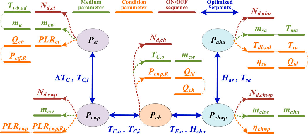
Figure 2. Interactions and connections among different types of components of HVAC system.

The description of the problem above indicates that the subproblems of diffusion and allocation possess a dual nature: they are both independent and interconnected. To accomplish system optimization, cooperation between these sub - problems is essential. Given the distinct characteristics of these sub - problems, a multi - agent system can be utilized to allocate them among different agents, thereby simplifying the global optimization challenge, as illustrated in Figure 3. In this configuration, each individual agent is responsible for handling the allocation task at a local level. Simultaneously, the diffusion task is resolved through joint efforts among all the agents.

Figure 3

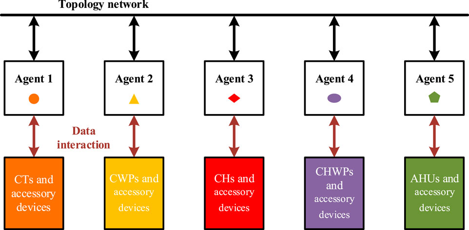
Figure 3. The task allocation in HVAC system under different network framework considering multi-agent.

3.2 Optimization model for HVAC systems based on multi-agent

Based on the optimization problem presented in Section 3.1, its optimization problem can be described in the compact form as follow Equation 26 after considering multi-intelligent agents.

$\begin{array}{l}\min \left[f_{Diffu}\left(X_{con}\right)+{\sum }_{mix}{f}_{alloca}\left(X_{dis,mix}\right)\right]\\ \mathrm{s}.\mathrm{t}.X\in {\cap }_{mix}{C}_{mix}\end{array}(26)$

where X is the set of decision variables, including the set point (X_con) and the on/off sequence (X_dis); f is the agent local objective function; and C_mix is the local constraints.

The concept of a coordinating agent is introduced to guarantee information synchronization among the intelligent agents of components. This coordinating agent holds equal priority with other component agents and is primarily tasked with solving the diffusion optimization problem. Here, the BDI model serves to depict the cognitive and decision - making procedures of the agent. In this model, beliefs signify the agent’s perception of the environment and the system’s state. Desires stand for the agent’s local aims and preferences, while intentions refer to the specific actions the agent undertakes based on its beliefs and desires. Regarding the coordinating agent, its beliefs can be regarded as a model of the coupling between diverse components. It updates its state according to the environmental parameters it receives from adjacent agents. The desires of the coordinating agent are local goals that, based on a concise version of the global optimization problem, can be expressed as Equation 27. The intention of the coordinating agent is defined as the action it takes to achieve its goal, and this can be formulated as Equation 28.

$\left\{\begin{array}{l}\min \left[f_{Diffu}\left(X_{con}\right)+P_f\left(X_{con}\right)\right]\\ \mathrm{s}.\mathrm{t}.L_{\mathit{min}}\le X^{*}\le L_{\mathit{max}},\end{array}\right.(27)$

$X_{con}^{\left(t+1\right)}=\arg \underset{X_{con}\in C}{\min }\left[f_{Diffu}\left(X_{con}^{\left(t\right)}{Z}_{con}^{\left(t\right)}\right)+P_f\left(X_{con}^{\left(t\right)}{Z}_{con}^{\left(t\right)}\right)\right](28)$

where $f_{Diffu}$ is a local objective function of the coordination agent; $P_f$ is an agent term, i.e., a penalized infeasible solution based on the information of neighboring components, and $Z_{con}$ is an information set constructed based on the coupling variables of neighboring components, which contain updated solutions from neighboring components.

Component agents are responsible for solving the allocation problem within various components. The optimization model of component agents 1-5 is shown in Equation 29. Similarly, its iterative execution at t+1 is represented as Equation 30.

$\left\{\begin{array}{l}\min \left[f_{Alloca,mix}\left(X_{dis,mix}\right)+P_{f,mix}\left(X_{dis,mix}\right)\right]\\ \mathrm{s}.\mathrm{t}.N_{d,mix}\ne \left\{0\right\}\&s_{mix,\mathit{min}}\le s_{mix}\le s_{mix,\mathit{max}}\end{array}\right.(29)$

$X_{dis,mix}^{\left(t+1\right)}=\arg \underset{X_{dis,mix}\in C}{\min }\left[f_{Alloca}\left(X_{dis,mix}^{\left(t\right)}{Z}_{dis,mix}^{\left(t\right)}\right)+P_{f,mix}\left(X_{dis,mix}^{\left(t\right)}{Z}_{dis,mix}^{\left(t\right)}\right)\right](30)$

$Z_{con}$ changes with each iteration of the algorithm, resulting in an update of $P_f$ and $f_{Diffu}$ at each iteration. This variable is crucial for agents to interact and update their decision variables. Here, $Z_{con}$ consists of the updated decision variables obtained from neighboring agents through communication as follow Equation 31. In addition, $Z_{dis}$ represents the set of information obtained from neighboring dissimilar component interactions as follow Equation 32.

$Z_{con}^{\left(t\right)}=\left\{X_{dis,ct}^{*,\left(t\right)},X_{dis,ch}^{*,\left(t\right)},X_{dis,chwp}^{*,\left(t\right)},\dots \right\}(31)$

$Z_{dis,mix}^{\left(t\right)}=\left\{X_{con}^{*,\left(t\right)}\right\}(32)$

In each iteration, the coordinating agent interacts with neighboring agents to obtain $Z_{con}$, and then uses the AH-AFSA algorithm to update its local state and evaluate its local adaptation $Y_{con}$. The fitness values of the coordinating agent and component agents are represented by Equations 33, 34, respectively.

$Y_{i,con}^{\left(t+1\right)}=\frac{1}{P_{sys}\left(X_{i,con}^{\left(t\right)}{Z}_{con}^{\left(t\right)}\right)+P_f\left(X_{i,con}^{\left(t\right)}{Z}_{con}^{\left(t\right)}\right)}(33)$

$Y_{i,dis,mix}^{\left(t+1\right)}=\frac{1}{P_{mix}\left(X_{i,dis,mix}^{\left(t\right)}{Z}_{dis,mix}^{\left(t\right)}\right)+P_{f,mix}\left(X_{i,dis,mix}^{\left(t\right)}{Z}_{dis,mix}^{\left(t\right)}\right)}(34)$

To ensure the optimality and consistency of the solution, all agents have to compute the global adaptation and local adaptation. First, each agent computes its local adaptation ($Y_{i,con}$ or $Y_{i,dis,mix}$) based on the current environment and broadcasts this information to its neighbors. Then, after receiving the local adaptations from neighboring agents, the global adaptation is computed as follow Equation 35. The local adaptability helps the agent to determine the best role for each type of component. Global adaptability allows agents to choose the best combination of component types to use, thus ensuring that all agents move towards the globally optimal solution.

$F_i^{\left(t+1\right)}=Y_{i,con}^{\left(t+1\right)}\left(X_{i,con}^{\left(t+1\right)}\right)+{\sum }_{mix}{Y}_{i,dis,mix}^{\left(t+1\right)}\left(X_{i,dis,mix}^{\left(t+1\right)}\right)(35)$

When solving the optimization problem proposed in this paper, the solution of hybrid variables must be considered first.

The Continuous Artificial Fish Swarm Algorithm (C-AFSA) is a swarm intelligence algorithm for continuous-variable optimization, whose core principle is to achieve search by simulating the foraging, swarming, and following behaviors of fish schools. In continuous space, the algorithm randomly explores new positions within the visual range through the “swarming behavior” and moves in that direction if the fitness is better. It calculates the central position of the swarm through the “swarming behavior” and moves toward the center if the central fitness is better than the current one and not crowded, so as to enhance global exploration. The “following behavior” prompts individuals to follow the nearby optimal solution to accelerate local convergence. Key parameters such as Visual (determining the search breadth) and Step (controlling the movement amplitude) jointly balance the exploration and exploitation capabilities of the algorithm, while the fitness function is directly linked to the target problem (such as energy consumption minimization) to guide the search direction.

However, C-AFSA has significant limitations. First, its design is only for continuous variables and cannot directly handle discrete decisions (such as equipment start/stop states). It requires indirect modeling through continuous approximation (e.g., 0-1 coding), leading to accuracy loss. Second, in high-dimensional optimization, the search space expands exponentially (curse of dimensionality), causing a sharp decline in computational efficiency. Third, it has high parameter sensitivity. Fixed settings of step size and visual range easily lead to premature convergence or slow convergence.

The Discrete Artificial Fish Swarm Algorithm (D-AFSA), specifically designed for discrete variables, maps problems to discrete spaces through discrete coding strategies such as binary or integer encoding. Its core behaviors are similar to those of C-AFSA, but the movement rules are adjusted to discrete jumps. For example, 1) Equipment start/stop states are represented by binary encoding (0/1). 2) The “swarming behavior” adjusts switch combinations via a majority voting mechanism. 3) The “following behavior” selects the optimal coding sequence within the neighborhood.

D-AFSA also has prominent limitations. First, continuous variables must be discretized (e.g., temperature segmentation and quantization), leading to information loss and approximation errors. Second, searches in discrete spaces are prone to getting stuck in local optima, especially when the number of variable dimensions is high—the combinatorial explosion problem significantly reduces search efficiency. Third, similar to C-AFSA, parameter settings have a significant impact on algorithm performance, and it lacks dynamic adaptability.

The inadequate handling of hybrid variables is a common bottleneck for both types of algorithms. Optimization problems in real-world systems (such as HVAC) often involve hybrid variables (e.g., continuous flow settings and discrete equipment on/off states), which cannot be cooperatively handled by either C-AFSA or D-AFSA. If a hybrid problem is forcibly split into continuous and discrete subproblems for separate optimization, additional coordination mechanisms are required to avoid solution space fragmentation, and suboptimal solutions are likely due to ignored interactions. For example, if the coupling between cooling tower on/off (discrete) and water pump flow (continuous) in HVAC is optimized independently, local decision conflicts may reduce overall energy efficiency. Furthermore, both algorithms rely on fixed parameters and struggle to adapt to dynamic load changes, further limiting their practical applications.

To address these shortcomings, this paper proposes an Adaptive Hybrid Artificial Fish Swarm Algorithm (AH-AFSA) in the next section. Through a hybrid variable fusion and divide-and-conquer strategy, adaptive mechanisms, and a collaborative framework, AH-AFSA not only solves the challenge of hybrid variable handling but also significantly enhances the robustness and real-time performance of complex system optimization, providing a more efficient solution for multi-variable coupling scenarios like HVAC.

4 Solution based on adaptive hybrid AFSA

Aiming to address mixed collaborative optimization problems for HVAC systems, it is necessary to optimize both continuous and discrete decision variables simultaneously. Therefore, this paper proposes an AH-AFSA algorithm, which inherits the advantages of C-AFSA and D-AFSA. When handling problems with continuous decision variables, such as diffusion problems, C-AFSA is a more appropriate choice. On the other hand, D-AFSA is appropriate for problems where discrete decision variables are involved, for example, allocation problems. It consists of four main steps: initialization, predation, swarming and following. The step size and visual of AH-AFSA is represented in $visual=\left\{visua{l}_{con},visua{l}_{dis}\right\}$ and $step=\left\{ste{p}_{con},ste{p}_{dis}\right\}$.

In the initialization phase, several parameters including fish group M, maximum number of attempts $N_{try}$, dimension n, vision, step size, feasible solution space L, maximum number of moves T, and crowding factor $\delta$ are required to be initialized. And each fish i $\left(X_i\right)$ contains two types of segments, one segment is a continuous part $X_{i,con}$, and the other is a discrete part $X_{i,dis}$. Each segment has its own dimension, and the sum of the dimensions of all segments is the dimension of the artificial fish. The initialization process is shown in Equation 36:

$\begin{array}{ll}\hfill X_i^{\left(0\right)}& =\left(X_{i,con}^{\left(0\right)},X_{i,dis}^{\left(0\right)}\right)=\left(\begin{array}{l}{x}_{i,con,1}^{\left(0\right)},x_{i,con,2}^{\left(0\right)},\cdots ,x_{i,con,d}^{\left(0\right)},\cdots ,x_{i,con,n}^{\left(0\right)},\\ x_{i,dis,1}^{\left(0\right)},x_{i,dis,2}^{\left(0\right)},\cdots ,x_{i,dis,k}^{\left(0\right)},\cdots ,x_{i,dis,m}^{\left(0\right)}\end{array}\right),\hfill \\ \hfill & x_{i,dis,k}\in \left\{0,1\right\},k=1,2,\cdots ,m\hfill \end{array}(36)$

During the feeding phase, the fish i will randomly choose newly position j within the field of view $\left(d_{i,j}<visual\right)$ as follow Equation 37. If the fitness of $X_j$ is better than $X_i$, then fish i will move one step toward position j as follow Equations 38, 39.

$X_j=X_i+visual·rand\left(-1,1\right)(37)$

$x_{i,con,d}^{\left(t+1\right)}=x_{i,con,d}^{\left(t\right)}+\frac{x_{j,con,d}-x_{i,con,d}^{\left(t\right)}}{d_{i,j}}·set{p}_{con}·rand\left(0,1\right)(38)$

$x_{i,dis,k}^{\left(t+1\right)}=\left\{\begin{array}{cc}\begin{array}{ll}{x}_{j,dis,k}& x_{i,dis,k}^{\left(t\right)}=x_{j,dis,k}\\ \mathit{min}\left(1,x_{j,dis,k}\right)& x_{i,dis,k}^{\left(t\right)}\ne x_{j,dis,k}\end{array}& k=RAND\left(1,n,ste{p}_{dis}\right)\end{array}\right.(39)$

where $X_j=\left(x_{j,con},x_{j,dis}\right)$, RAND (1, n, step) denotes a randomly generated integer between 1 and n, and t denotes the tth move. If fish i does not find a suitable prey target after the second attempt, it will take a random move as follow Equations 40, 41.

$x_{i,con,d}^{\left(t+1\right)}=x_{i,con,d}^{\left(t\right)}+set{p}_{con}·rand\left(-1,1\right)(40)$

$x_{i,dis,k}^{\left(t+1\right)}=\left\{\begin{array}{cc}\begin{array}{cc}0& x_{i,dis,k}^{\left(t\right)}=1\\ 1& x_{i,dis,k}^{\left(t\right)}=0\end{array}& k=RAND\left(1,n,ste{p}_{dis}\right)\end{array}\right.(41)$

In the group stage, fish i will sense the number of companions ($n_f$) within the field of view and the center of the group (c), and the center of the group $X_c$ can be expressed as Equations 43, 44, and if the adaptation of is better and the center is not congested, fish i will move to the center as follow Equations 45, 46. The preconditions for the group action are shown in Equation 42, and if the conditions are not satisfied, the predation action is carried out.

$\frac{n_f}{N}<\delta \&Y_c>Y_i(42)$

$x_{c,con,d}=\frac{{\sum }_{j=1}^{n_f}{x}_{j,con,d}}{n_f}(43)$

$x_{c,dis,k}=round\left({\sum }_{j=1}^{n_f}{x}_{j,dis,k}/n_f\right)(44)$

$x_{i,con,d}^{\left(t+1\right)}=x_{i,con,d}^{\left(t\right)}+\frac{x_{c,con,d}-x_{i,con,d}^{\left(t\right)}}{d_{i,c}}·set{p}_{con}·rand\left(0,1\right)(45)$

$x_{i,dis,k}^{\left(t+1\right)}=\left\{\begin{array}{cc}\begin{array}{ll}{x}_{c,dis,k}& x_{i,dis,k}^{\left(t\right)}=x_{c,dis,k}\\ \mathit{min}\left(1,x_{c,dis,k}\right)& x_{i,dis,k}^{\left(t\right)}\ne x_{c,dis,k}\end{array}& k=RAND\left(1,n,ste{p}_{dis}\right)\end{array}\right.(46)$

In the following phase, fish i senses the best adapted companion b within its field of view, and if the adaptation $X_b$ is better and there are no crowded fish in the vicinity, fish i moves one step towards the companion b as follow Equations 48, 49. If the condition of following action as follow Equation 47 is not satisfied, the predation action is performed.

$\frac{n_f}{N}<\delta \&Y_b>Y_i(47)$

$x_{i,con,d}^{\left(t+1\right)}=x_{i,con,d}^{\left(t\right)}+\frac{x_{b,con,d}-x_{i,con,d}^{\left(t\right)}}{d_{i,k}}·set{p}_{con}·rand\left(0,1\right)(48)$

$x_{i,dis,k}^{\left(t+1\right)}=\left\{\begin{array}{ll}\begin{array}{ll}{x}_{b,dis,k}& x_{i,dis,k}^{\left(t\right)}=x_{b,dis,k}\\ \mathit{min}\left(1,x_{b,dis,k}\right)& x_{i,dis,k}^{\left(t\right)}\ne x_{b,dis,k}\end{array}& k=RAND\left(1,n,ste{p}_{dis}\right)\end{array}\right.(49)$

In an effort to boost the local search ability and the convergence rate of AH-AFSA, this paper formulates the concept of action reward and modifies the fixed step - size to an adaptive one. The action reward R is specified as the gain that fish i attains when moving towards target o, as presented in Equation 50. The step size of the action is defined in accordance with Equation 51:

$R=\frac{Y_o-Y_i}{Y_o}(50)$

$step=ste{p}_{\mathit{min}}+\left(ste{p}_{\mathit{max}}-ste{p}_{\mathit{min}}\right)·R(51)$

where $ste{p}_{\mathit{min}}$ and $ste{p}_{\mathit{max}}$ are the bounds of the step size.

5 Case studies

5.1 Case background

The system of the case studies analysis is built upon the HVAC system of a public building. This building has an air-conditioned area of 49,000 square meters and a total floor area of 55,000 square meters. The HVAC system consists of 4 AHUs, 3 CTs, 3 CWPs, 3 CHWPs and 3 CHs. Table 1 show the components’ detailed specifications. Based on 70% identification data and 30% validation data, Tables 2, 3 present the parameter identification results for the model proposed in this paper. Under this system configuration, component agents numbered from 1 to 5 are integrated with component models of AHUs, CHWPs, CHs, CWPs and CTs respectively. Its main task is to tackle the allocational optimization problem. On the other hand, coordination agents are furnished with component interaction models and is mainly concentrated on addressing diffusional optimization problems.

Table 1

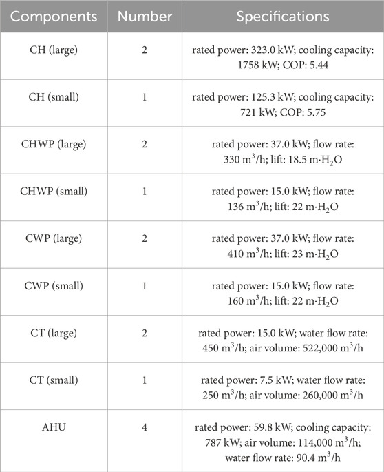
Table 1. Specifications of the main components of the HVAC system.

Table 2

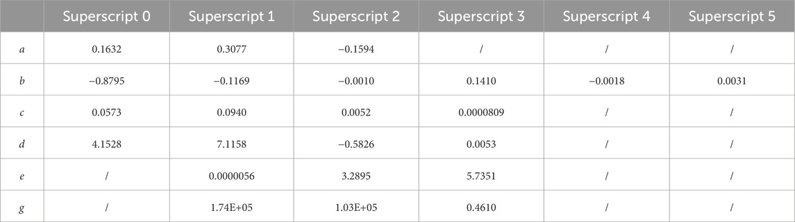
Table 2. Model identification results of the large components.

Table 3

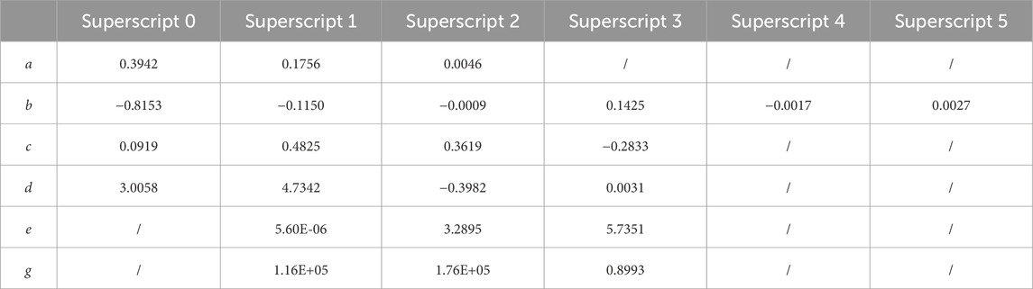
Table 3. Model identification results of the small components.

5.2 Comparison analysis for distinct optimization approaches

To conduct a comprehensive assessment of the performance of the proposed approach, a comparison analysis taking into account energy consumption and computational efficiency across the diverse operating condition will be carried out. The following four approaches’ performance will be contrasted:

(1) Approach 1: a traditional approach based on constant for optimizing the system, i.e., x₅ ∼ x₁₀ set magnitudes is respectively 7°C, 22 m·H₂O, 5°C, 30°C, 18°C, and 900 Pa;

(2) Approach 2: an intelligent optimization approach based on AHDE for optimizing the set magnitudes;

(3) Approach 3: an artificial fish swarm optimization algorithm considering continuous variables (C-AFSA);

(4) Approach 4: the method proposed in this paper (AH-AFSA).

5.2.1 Analysis of the hourly power consumption of the HVAC system over three representative days

Figure 4 depicts hourly power consumptions of the HVAC system under three typical days, operating conditions as per Figure 5, when four optimization approaches are applied. Evidently, power consumptions of the approach based on constant is substantially greater than the others, particularly in high cooling loads period, which ranges from 9:00 a.m. to 14:00 p.m. Highlighting the remarkable energy conservation performance of variables set magnitudes optimization approaches.

Figure 4

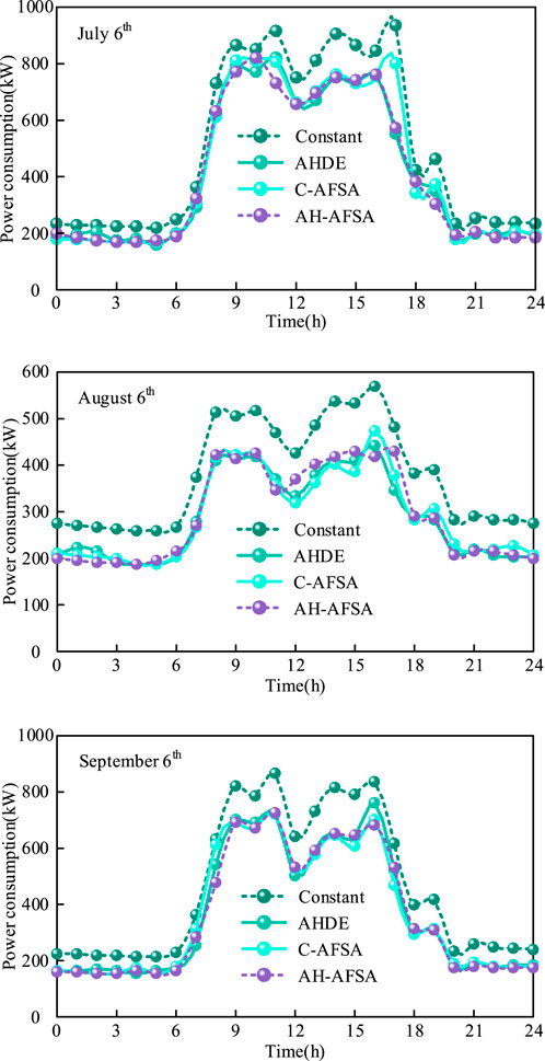
Figure 4. Hourly total power of the HVAC system in the three typical days.

Figure 5

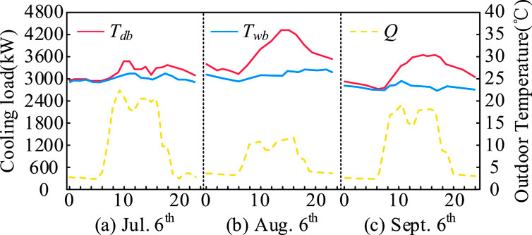
Figure 5. Outdoor climate and cooling load in the three typical days.

5.2.2 Analysis of cooling loads and outdoor climate during three representative days

Figure 6 shows total power consumptions of the HVAC system across three representative periods. The “Relative Savings” entry indicates energy conservations of AH-AFSA approach in relation to others. Compared to the constant approach, the AH-AFSA approach attains relative energy conservations ranging from 13.3 percent to 17.7 percent. In contrast to the C-AFSA and AHDE approaches, the maximum relative energy conservations are 1.0 percent and 2.4 percent respectively. In addition, energy conservations potential of AH-AFSA approach is marginally greater than that of the C-AFSA and AHDE approaches. Above enhancements can be ascribed to the disparities in dealing with discrete decision variables among three algorithms, with the C-AFSA and AHDE algorithms using Sysconvert and circular methods to optimize the discrete decision variables, which results in a loss of accuracy in the discrete variables. The above superiority of AH-AFSA will become more evident in larger HVAC systems with more homogeneous components.

Figure 6

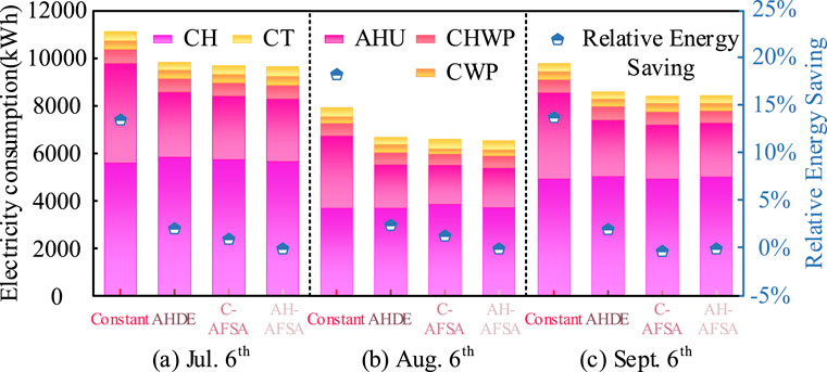
Figure 6. Outdoor climate and cooling load in the three typical days.

5.2.3 Analysis of subitems in HVAC system power consumption during annual cooling seasons

Figure 7 depicts the annual power consumption in the HVAC system corresponding to various optimization approaches. The percentages presented therein signify the proportion of energy conservations that the AH-AFSA approach achieves in comparison to other approaches within each identical subitem. Annual power consumption levels of above three approaches are quite similar. In terms of energy conservations, the AH-AFSA approach shows relative conservations of 2.5 percent and 0.9 percent when contrasted with the traditional constant approach. When compared to the C-AFSA and AHDE approaches respectively, the relative conservations of the AH-AFSA method can reach as high as 18.9%. Regarding the power consumption for CH, AHU and CHWP, in comparison with other approaches, the relative energy conservations achieved by the AH-AFSA approach were 19.6%, 24.0%, and 13.2% respectively. Although, with respect to CT and CWP, the power consumption of AH-AFSA is marginally greater than the constant method, this goes against the common anticipation that the energy consumption of every component would decline. This divergence occurs since the goal of the research in this paper is to find the optimal result for the overall HVAC system by taking into account the trade-off features between the components. When considering the energy efficiency in total, it proves more advantageous to moderately augment the flow of cooling water and the air flow in the cooling tower. By adopting this approach, the overall energy efficiency of the HVAC system can be elevated. Results from the analysis further implies that the proposed approach is able to reach overall optimization through striking a balance in energy efficiency among individual components and the entire HVAC system, giving up the energy efficiency of some part of components like CWPs and CT fans in HVAC system.

Figure 7

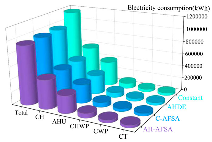
Figure 7. The subitems of the system electricity consumption in the annual cooling season.

5.3 Comparative analysis of calculation efficiency and calculation time of different methods

The comparison analysis of three different methods, from the perspective of computing efficiency, consider iteration times and computational times shown in Figure 8, respectively.

Figure 8

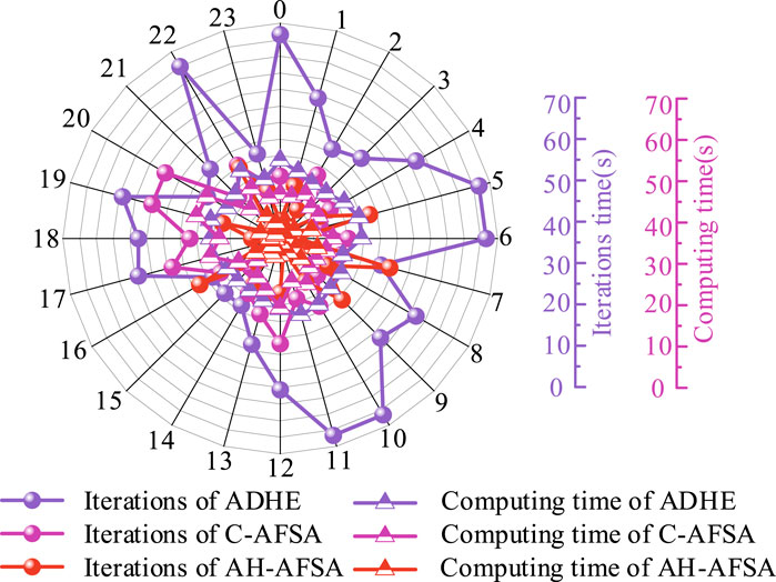
Figure 8. Iterations and time cost of different methods in a typical day.

As shown in Figure 8, during the optimization process, the AHDE method requires a relatively large number of iterations, ranging from twenty to seventy, when contrasted with the other two approaches. Simultaneously, the disparity in the iteration numbers of AH-AFSA and C-AFSA is not significant, remaining in the range of approximately 40 iterations. In addition, under certain operational conditions, the iteration numbers of AH - AFSA are restricted to 10. This indicates that the efficiency of AH - AFSA is marginally superior to C - AFSA. In contrast, since AH-AFSA doesn't incorporate an approximate circular procedure, it proves to be more effective when addressing integer program problems such as switching sequences. It can be noted that the AH - AFSA algorithm requires the least amount of time to reach the optimal solution. Furthermore, it can be noted that the AH-AFSA requires the least amount of times to reach the optimum effect. In the case of the AHDE algorithm, the time taken for computations across all operating points spans from 18 to 25 s. On average, each operating point demands 21 s of computational time. Under the majority of operating conditions, the iterations of AH - AFSA can be wrapped up within 10 s. Meanwhile, the computational time for C - AFSA varies between 10 and 27 s. Even though the variation in the number of iterations between the C - AFSA and AH - AFSA algorithms isn't substantial, C - AFSA exhibits a relatively longer computation time. This clearly shows that AH - AFSA boasts higher computational efficiency. Despite the fact that, within this research, the basic parameter configurations for the C - AFSA and AH - AFSA algorithms are identical, the application frameworks of these two algorithms diverge significantly. As a result, the data presented in Figure 8 also implies that algorithms can be enhanced effectively within a multi - agent framework, with a relatively minimal time expense for each iteration.

5.4 In-depth analysis of influencing factors

5.4.1 Analysis of the coupling strength of cooling water temperature and cooling tower airflow weights

This paper focuses on the influence of the interaction weights of cooling water temperature and airflow on energy consumption in HVAC systems. By studying the distribution of total energy consumption under different interaction weights, we aim to clarify the internal correlation and provide a basis for the optimization of system energy consumption.

From Figure 9, we can clearly see the performance of energy consumption with different values of interaction weights. When the interaction weights $\alpha$ are 0.2, 0.4, 0.6, 0.8 and constant control (control group), the distribution of energy consumption shows significant differences. At an interaction weight $\alpha$ of 0.6, the distribution of energy consumption is more prominent. Its average energy consumption (marked by squares) and median (marked by horizontal lines) are relatively low, and the degree of data dispersion is small, indicating that under this weight, the HVAC system operates relatively stable, with less fluctuation in energy consumption. This verifies that within a certain range, a reasonable interaction weight can effectively improve the system energy efficiency and reduce unnecessary energy loss. With the deviation of the interaction weights towards the ends of 0.2 and 0.8, the distribution of energy consumption changes significantly. When $\alpha$ = 0.2, the energy consumption data points are more dispersed, which indicates that the system operation stability is poor, probably due to the improper setting of weights, resulting in the deviation of the system in adjusting the cooling water temperature and airflow, which leads to the increase of energy consumption fluctuation. When $\alpha$ = 0.8, although there are some lower energy consumption data, there are also some outliers with higher energy consumption, which implies that under high weights, the system may focus too much on the regulation of one factor while neglecting another factor, resulting in an imbalance in the overall energy consumption control. The control group (constant control) has a significantly higher level of energy consumption than the other cases under different weight settings. Its average energy consumption and median are at a high level, and the wide distribution of data points reflects the limitations of the traditional constant control method in dealing with the complex working conditions of the system, which highlights the necessity of optimizing control based on multi-agent consideration of interaction weights.

Figure 9

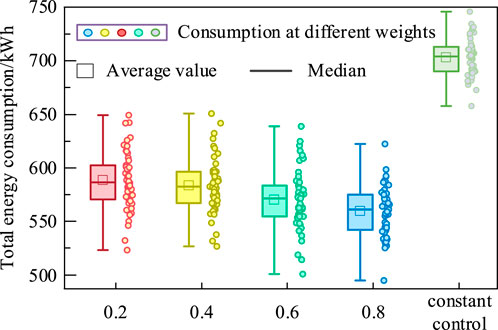
Figure 9. Analysis of the coupling strength of cooling water temperature and cooling tower airflow weights.

5.4.2 Analysis of AH-AFSA parameter sensitivity testing

Figure 10 investigates the two key parameters of AH-AFSA algorithm: visual range and adaptive step range. The average daily energy consumption of the HVAC system in the traditional method (e.g., constant setting value) is about 1,200∼1,500 kW h, while the energy consumption is reduced to 950∼1,200 kW h after AH-AFSA optimization (saving about 18.9%). When the value of the system parameter field of view is 0.1–0.5 and the adaptive step range is 0.3–0.7, the HVAC system shows a clear distribution of low energy consumption in the middle and high energy consumption at both ends. When the field of view range is about 0.3 and the adaptive step range is about 0.5, it is at the lowest point of the energy consumption surface, which corresponds to the lowest energy consumption, about 954.6 kW h, which indicates that the algorithm energy consumption optimization is the best under this parameter combination. When the field of view range and adaptive step range deviate from the optimal parameter combination of 0.3 and 0.5, the energy consumption gradually climbs to a higher level of about 1,200 kW h, which indicates that the deviation of this parameter combination leads to an increase in the energy consumption of the HVAC system. The closer to the optimal parameter combination area, the faster the energy consumption decreases, which means that reasonable adjustment of the parameter visual range and Adaptive step range, so that the value is close to the optimal combination, can effectively reduce the energy consumption of the HVAC system, and vice versa will lead to an increase in energy consumption, but also reflects the synergistic operation of the trade-off between the components of the HVAC system. It also reflects the effectiveness of the trade-off between the synergistic operation of the HVAC system components to reduce the energy consumption of the HVAC system.

Figure 10

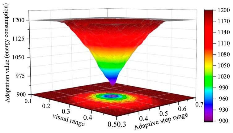
Figure 10. Analysis of visual range and adaptive step range parameter sensitivity testing.

6 Conclusion

This paper presents a collaborative optimization approach based on multi-agent. By taking into account the interaction traits between components of HVAC systems, this approach aims to solve the energy efficiency trade-off problem in the complicated HVAC system that consist of homogeneous components with different capacities. To prove the effectiveness of this proposed approach, arithmetic examples from practical HVAC systems are analyzed. As a result, the following conclusions can be derived:

(1) The approach presented in this paper breaks down a complicated optimization problem into multiple straightforward subproblems, which are then resolved in an efficient manner. Moreover, it possesses strong reconfigurability, allowing it to adapt to HVAC systems featuring varying degrees of complexity and diverse optimization goals.

(2) From the perspective of the energy conservation potential, the multi-agent based collaborative optimization approach for HVAC systems proposed in this study has the capacity to reduce power consumption by approximately 18.9 percent in contrast to traditional approaches. When compared with other intelligent approaches such as those based on AHDE and C-AFSA, their respective relative energy conservation rates are merely 2.5 percent and 0.9 percent.

(3) When it comes to computing efficiency, the AH-AFSA algorithm based on multi-agent proposed in this study clearly surpasses the centralized C-AFSA algorithm. In contrast, the average computation time for AH-AFSA saves approximately 54 percent than the centralized framework.

Even though the validity of the proposed collaborative optimization method has been verified, its comparative analysis only covers traditional methods and those based on AFSA. In future works, more advanced methods within agent-based frameworks will be investigated, and its performances will be assessed by implementing in practical systems.

Data availability statement

The original contributions presented in the study are included in the article/Supplementary Material, further inquiries can be directed to the corresponding author.

Author contributions

CF: Funding acquisition, Methodology, Supervision, Writing – review and editing. KC: Writing – original draft. YX: Resources, Software, Visualization, Writing – review and editing. DM: Methodology, Supervision, Writing – review and editing. RY: Data curation, Resources, Writing – original draft. YW: Writing – original draft. LS: Conceptualization, Methodology, Writing – review and editing.

Funding

The author(s) declare that financial support was received for the research and/or publication of this article. This work was supported by Science and Technology Project of SGCC (Research and Application of Load Decomposition and Energy-saving Potential Assessment for Air Conditioning Load Based on Gate Measurement in Typical Public Buildings) (5400-202318574A-3-2-ZN).

Conflict of interest

Author RY was employed by State Grid Hubei Shiyan Power Supply Company.

The remaining authors declare that the research was conducted in the absence of any commercial or financial relationships that could be construed as a potential conflict of interest.

Generative AI statement

The author(s) declare that no Generative AI was used in the creation of this manuscript.

Publisher’s note

All claims expressed in this article are solely those of the authors and do not necessarily represent those of their affiliated organizations, or those of the publisher, the editors and the reviewers. Any product that may be evaluated in this article, or claim that may be made by its manufacturer, is not guaranteed or endorsed by the publisher.

Supplementary material

The Supplementary Material for this article can be found online at: https://www.frontiersin.org/articles/10.3389/fenrg.2025.1609210/full#supplementary-material

References

Afroz, Z., Shafiullah, G. M., Urmee, T., Shoeb, M. A., and Higgins, G. (2022). Predictive modelling and optimization of HVAC systems using neural network and particle swarm optimization algorithm. Build. Environ. 209, 108681. doi:10.1016/j.buildenv.2021.108681

CrossRef Full Text | Google Scholar

Cai, J., Kim, D., Jaramillo, R., Braun, J. E., and Hu, J. (2016). A general multi-agent control approach for building energy system optimization. Energy Build. 127, 337–351. doi:10.1016/j.enbuild.2016.05.040

CrossRef Full Text | Google Scholar

Cai, J., Kim, D., Putta, V. K., Braun, J. E., and Hu, J. (2015). “Multi-agent control for centralized air conditioning systems serving multi-zone buildings,” in 2015 American control conference (ACC) (Chicago, IL, USA: IEEE), 986–993. doi:10.1109/ACC.2015.7170862

CrossRef Full Text | Google Scholar

Cao, S.-J., and Ren, C. (2018). Ventilation control strategy using low-dimensional linear ventilation models and artificial neural network. Build. Environ. 144, 316–333. doi:10.1016/j.buildenv.2018.08.032

CrossRef Full Text | Google Scholar

Cheng, Y., Zhang, S., Huan, C., Oladokun, M. O., and Lin, Z. (2019). Optimization on fresh outdoor air ratio of air conditioning system with stratum ventilation for both targeted indoor air quality and maximal energy saving. Build. Environ. 147, 11–22. doi:10.1016/j.buildenv.2018.10.009

CrossRef Full Text | Google Scholar

Coelho, L. D. S., Klein, C. E., Sabat, S. L., and Mariani, V. C. (2014). Optimal chiller loading for energy conservation using a new differential cuckoo search approach. Energy 75, 237–243. doi:10.1016/j.energy.2014.07.060

CrossRef Full Text | Google Scholar

Coelho, L. D. S., and Mariani, V. C. (2013). Improved firefly algorithm approach applied to chiller loading for energy conservation. Energy Build. 59, 273–278. doi:10.1016/j.enbuild.2012.11.030

CrossRef Full Text | Google Scholar

Dos Santos Coelho, L., and Askarzadeh, A. (2016). An enhanced bat algorithm approach for reducing electrical power consumption of air conditioning systems based on differential operator. Appl. Therm. Eng. 99, 834–840. doi:10.1016/j.applthermaleng.2016.01.155

CrossRef Full Text | Google Scholar

Jang, Y.-E., Kim, Y.-J., and Catalao, J. P. S. (2021). Optimal HVAC system operation using online learning of interconnected neural networks. IEEE Trans. Smart Grid 12, 3030–3042. doi:10.1109/TSG.2021.3051564

CrossRef Full Text | Google Scholar

Kim, H., Hong, T., and Kim, J. (2019). Automatic ventilation control algorithm considering the indoor environmental quality factors and occupant ventilation behavior using a logistic regression model. Build. Environ. 153, 46–59. doi:10.1016/j.buildenv.2019.02.032

CrossRef Full Text | Google Scholar

Labeodan, T., Aduda, K., Boxem, G., and Zeiler, W. (2015). On the application of multi-agent systems in buildings for improved building operations, performance and smart grid interaction – a survey. Renew. Sustain. Energy Rev. 50, 1405–1414. doi:10.1016/j.rser.2015.05.081

CrossRef Full Text | Google Scholar

Lee, W.-S., Chen, Y.-T., and Kao, Y. (2011). Optimal chiller loading by differential evolution algorithm for reducing energy consumption. Energy Build. 43, 599–604. doi:10.1016/j.enbuild.2010.10.028

CrossRef Full Text | Google Scholar

Li, L., Fu, Y., Fung, J. C. H., Qu, H., and Lau, A. K. H. (2021). Development of a back-propagation neural network and adaptive grey wolf optimizer algorithm for thermal comfort and energy consumption prediction and optimization. Energy Build. 253, 111439. doi:10.1016/j.enbuild.2021.111439

CrossRef Full Text | Google Scholar

Li, W., Koo, C., Cha, S. H., Hong, T., and Oh, J. (2018). A novel real-time method for HVAC system operation to improve indoor environmental quality in meeting rooms. Build. Environ. 144, 365–385. doi:10.1016/j.buildenv.2018.08.046

CrossRef Full Text | Google Scholar

Li, W., and Wang, S. (2020). A multi-agent based distributed approach for optimal control of multi-zone ventilation systems considering indoor air quality and energy use. Appl. Energy 275, 115371. doi:10.1016/j.apenergy.2020.115371

CrossRef Full Text | Google Scholar

Li, Z., Guo, J., Gao, X., Yang, X., and He, Y.-L. (2023). A multi-strategy improved sparrow search algorithm of large-scale refrigeration system: optimal loading distribution of chillers. Appl. Energy 349, 121623. doi:10.1016/j.apenergy.2023.121623

CrossRef Full Text | Google Scholar

Ma, K., Liu, M., and Zhang, J. (2021). Online optimization method of cooling water system based on the heat transfer model for cooling tower. Energy 231, 120896, doi:10.1016/j.energy.2021.120896

CrossRef Full Text | Google Scholar

Majzoobi, L., Shah-Mansouri, V., and Lahouti, F. (2018). Analysis of distributed ADMM algorithm for consensus optimisation over lossy networks. IET signal process 12, 786–794. doi:10.1049/iet-spr.2018.0033

CrossRef Full Text | Google Scholar

Michailidis, I. T., Schild, T., Sangi, R., Michailidis, P., Korkas, C., Fütterer, J., et al. (2018). Energy-efficient HVAC management using cooperative, self-trained, control agents: a real-life German building case study. Appl. Energy 211, 113–125. doi:10.1016/j.apenergy.2017.11.046

CrossRef Full Text | Google Scholar

Salsbury, T. I., Devaprasad, K., Lutes, R., and Rogers, A. P. (2023). Smarter building start – a distributed solution. Energy Build. 282, 112776. doi:10.1016/j.enbuild.2023.112776

CrossRef Full Text | Google Scholar

Seo, J., Ooka, R., Kim, J. T., and Nam, Y. (2014). Optimization of the HVAC system design to minimize primary energy demand. Energy Build. 76, 102–108. doi:10.1016/j.enbuild.2014.02.034

CrossRef Full Text | Google Scholar

Seong, N.-C., Kim, J.-H., and Choi, W. (2019). Optimal control strategy for variable air volume air-conditioning systems using genetic algorithms. Sustainability 11, 5122. doi:10.3390/su11185122

CrossRef Full Text | Google Scholar

Wang, J., and Zhao, T. (2024). Medium spatiotemporal characteristics based global optimization method for energy efficiency trade-off issue in variable flow rate HVAC system. Appl. Therm. Eng. 247, 123132. doi:10.1016/j.applthermaleng.2024.123132

CrossRef Full Text | Google Scholar

Wang, Z., Wang, L., Dounis, A. I., and Yang, R. (2012). Multi-agent control system with information fusion based comfort model for smart buildings. Appl. Energy 99, 247–254. doi:10.1016/j.apenergy.2012.05.020

CrossRef Full Text | Google Scholar

Xiong, W., and Wang, J. (2020). A semi-physical static model for optimizing power consumption of HVAC systems. Control Eng. Pract. 96, 104312. doi:10.1016/j.conengprac.2020.104312

CrossRef Full Text | Google Scholar

Yang, R., and Wang, L. (2013). Development of multi-agent system for building energy and comfort management based on occupant behaviors. Energy Build. 56, 1–7. doi:10.1016/j.enbuild.2012.10.025

CrossRef Full Text | Google Scholar

Yu, H., Zhao, T., and Zhang, J. (2018). Development of a distributed artificial fish swarm algorithm to optimize pumps working in parallel mode. Sci. Technol. Built Environ. 24, 248–258. doi:10.1080/23744731.2017.1375011

CrossRef Full Text | Google Scholar

Zhang, X., Fong, K. F., and Yuen, S. Y. (2013). A novel artificial bee colony algorithm for HVAC optimization problems. HVAC&R Res. 19, 715–731. doi:10.1080/10789669.2013.803915

CrossRef Full Text | Google Scholar

Zhao, T., Wang, J., Fu, P., and Wu, X. (2021). Study on simplified energy-efficient control methods of HVAC cooling water system from the global online optimization perspective. Energy Sci. Eng. 9, 464–482. doi:10.1002/ese3.861

CrossRef Full Text | Google Scholar

Zheng, Z., and Li, J. (2018). Optimal chiller loading by improved invasive weed optimization algorithm for reducing energy consumption. Energy Build. 161, 80–88. doi:10.1016/j.enbuild.2017.12.020

CrossRef Full Text | Google Scholar

Zheng, Z., Li, J., and Duan, P. (2019). Optimal chiller loading by improved artificial fish swarm algorithm for energy saving. Math. Comput. Simul. 155, 227–243. doi:10.1016/j.matcom.2018.04.013

CrossRef Full Text | Google Scholar

Zhuang, D., Gan, V. J. L., Duygu Tekler, Z., Chong, A., Tian, S., and Shi, X. (2023). Data-driven predictive control for smart HVAC system in IoT-integrated buildings with time-series forecasting and reinforcement learning. Appl. Energy 338, 120936. doi:10.1016/j.apenergy.2023.120936

CrossRef Full Text | Google Scholar