Coordinated multi-level scheduling method considering uncertainty of renewable energy and load

As renewable energy continues to be widely integrated, the energy structure is gradually transforming. The increasing grid connection of wind and photovoltaic power signifies a major shift in the energy mix. This change is particularly evident in heavy load areas at the regional grid and provincial dispatch levels, where uncertainties on both the supply and demand sides impact the daily operation of power systems. New dispatch strategies are urgently needed to address these uncertainties. This paper introduces a two-stage day-ahead and intra-day coordinated multi-level dispatch method that considers both the regional-level and provincial-level power systems, addressing supply-demand uncertainties from the perspective of regional grid-level and unmet load peak shaving. Unmet load refers to the load that cannot be met solely by the output of regional grid units. At the regional grid level, a unit dispatch model for unmet load peak shaving is developed. We introduce the concept of unmet load and, based on peak-valley weighting, propose a multi-province load peak shaving method, improving the approach to unmet load considerations. At the provincial level, a two-stage robust optimization dispatch model is constructed based on regional grid dispatch, and it is solved using the Karush-Kuhn-Tucker conditions and the Column-and-Constraint Generation (C&CG) algorithm. Finally, case study results validate the proposed model’s effectiveness, demonstrating its ability to provide an optimized coordinated grid-provincial dispatch strategy under supply-demand uncertainty.

1 Introduction

In the current context of widespread integration of renewable energy, considering the high degree of new energy integration in large-scale grid dispatch, the system is prone to fluctuations due to load and the variability in wind and solar power outputs, and is more susceptible to peak load situations, increasing the risk to power safety. It is particularly crucial to consider dispatch strategies at both regional grid and provincial levels to ensure power balance during peak load periods and to coordinate regional and provincial dispatch strategies. This aims to ensure stable power supply at the regional grid level and promote the consumption of new energy at the provincial level, thereby maximizing the safety of large-scale power grids.

At the regional grid level, the impact of new energy is significantly amplified due to the integration of multi-provincial loads, making it highly likely to encounter peak load situations during daily operations. Taking the East China Grid as an example, which mainly supplies power to Shanghai, Jiangsu, Zhejiang, Fujian, and Anhui, the daily power supply pressure is substantial, and it frequently participates in inter-provincial power dispatch (Li et al., 2024). Considering the limitations of line capacity and the cost of power adjustments in conventional units, using energy storage systems for cross-time scale power dispatch is an effective solution. Energy storage offers flexibility, efficiency, adjustability, rapid response, and environmental friendliness. Liu and Peng (2024) proposes a peak load transfer optimization model for wind-power-energy hybrid energy system based on situational awareness theory. Uddin et al. (2018) discusses on possible challenges and future research directions for each type of the strategy. Chua et al. (2016) provide an effective sizing method and an optimal peak shaving strategy for an energy storage system to reduce the electrical peak demand of the customers. Luo et al. (2024), Zhao et al. (2024), Cheng et al. (2018); Liao et al. (2024) construct different short-term peak-shaving frameworks to address the modeling challenge and optimization difficulty. Wallberg et al. (2024) presents a control algorithm that uses a negative correlation scheme, adjusted to the local grid load, to effectively manage the battery energy storage. Jin et al. (2022) uses flexible hydropower to buffer the volatility and the randomness of RE sources and aid peak shaving in response to the transition towards sustainability. Wang et al. (2021) proposes a nonlinear programming model to solve this problem. The research on energy storage for peak shaving is well-established, yet there is limited focus on regional grid-level dispatch scenarios. This paper takes into account the common issue of insufficient unit output at the regional grid level and considers the resulting unmet load situations. By utilizing energy storage systems to perform peak shaving and valley filling across multiple provinces, this study extends the objectives of peak shaving and valley filling to include reducing the fluctuations in unmet load.

At the provincial dispatch level, the main responsibility lies in accommodating the consumption of new energy after implementing unmet load peak shaving at the regional grid level. Dong et al. (2024) studies the operation and scheduling problem of virtual power plant with the collaborative optimization of multiple flexible loads and new energy, and improves the mismatch between power supply and demand through the efficient aggregation and optimal control of new energy and demand-side resources. Yang et al. (2024) designs a two-stage scheduling optimization framework to minimize the operating cost in the day-ahead phase and the system deviation cost in the intra-day phase. However, given the increasingly complex operational environment and various uncertainties, traditional optimization methods often fall short of meeting practical operational needs. The two-stage robust optimization method, an emerging optimization technology, has garnered considerable attention in recent years. This method has broad applicability in the field of power systems, whether in power market design, generation dispatch, or grid planning. By incorporating the two-stage robust optimization approach, complex issues in actual operations can be effectively addressed. Especially in the areas of new energy grid integration and inter-regional power trading, this method can effectively overcome challenges posed by uncertainties, ensuring efficient operation of the power system and optimal resource allocation. Zhao and Guan (2015) develops stochastic optimization models and solution methods to improve reliability unit commitment run practice. Büsing and Schmitz (2024), Zhu et al. (2024), Niu et al. (2022), Wang et al. (2022), Kong et al. (2022) study different two-stage robust optimization method under uncertainty of different variables. Zeng and Zhao (2013) present a column-and-constraint generation algorithm to solve two-stage robust optimization problems. Yang et al. (2023) proposes a distributed robust optimal scheduling method for microgrid based on discrete scenarios. Bendotti et al. (2023) proposes the anchor-robust approach as a middle ground between guaranteeing starting times and guaranteeing the thought.

This paper primarily introduces a two-stage robust optimization model under the coordination of regional grid-level dispatch. Based on regional grid dispatch strategies, it considers provincial dispatch under the influence of new energy sources. It also takes into account constraints such as tie-line power and inter-provincial electricity trading, aiming to minimize economic costs. The solution is obtained through iterative calculations.

2 Materials and methods

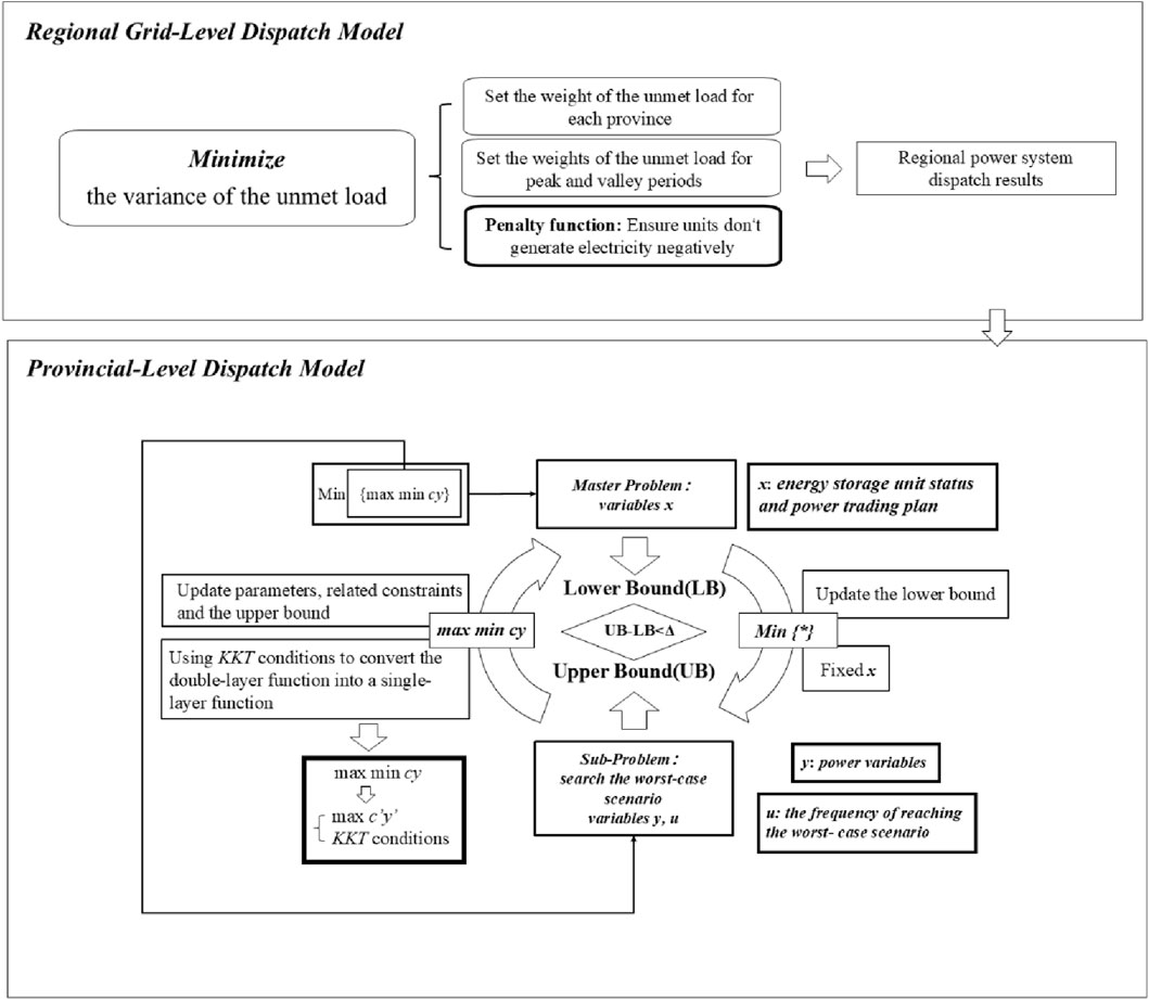
Figure 1 shows the model architecture in this document.

Figure 1

Figure 1. Model framework diagram.

2.1 Model formulation

2.1.1 Regional grid-level dispatch model

The dispatch optimization problem at the regional grid level studied in this paper involves two types of units: conventional generation units and pumped-storage power stations. The main constraints can be categorized as follows:

Controllable Conventional Unit Constraints:

Ramping Constraint Equation 1:

$-R{U}_g\le P_{g,p,t+1}-P_{g,p,t}\le R{U}_g(1)$

In the formula, t denotes the time period index, and p represents the province index. $P_{g,p,t+1},P_{g,p,t}$ are the generation power at time t+1 and t respectively. $R{U}_g$ represents the ramp rate limit of the thermal power unit, indicating the maximum increase or decrease in output per unit time.

Unit Output Boundary Constraint Equation 2:

$0\le P_{g,p,t}\le {P_g}^{\max }(2)$

In the formula, ${P_g}^{\max }$ denotes the maximum output of the unit, and the constraint is defined with a zero lower bound, which applies to the generation stage of all units.

Pumped-Storage Unit Constraints Equations 3–7:

Pumped-Storage Unit Equality Constraints, including water level conversion power constraint and power balance constraint:

${\eta }_{ch\arg e}\Delta E=P_{ch\arg e}t={\eta }_{ch\arg e}mg\Delta h(3)$

$\begin{array}{l}\Delta E={\eta }_{disch\arg e}{P}_{disch\arg e}t\\ ={\eta }_{disch\arg e}\times \left(mg+\frac{1}{2}\rho V^{2}S\right)\times \Delta h\end{array}(4)$

$E_{t+1}=E_t+\left({P_t}^{ch\arg e}{\eta }_{ch\arg e}+\frac{P_t^{disch\arg e}}{{\eta }_{disch\arg e}}\right)\Delta t(5)$

The boundary constraints of pumped -storage units include energy boundary constraints as well as pumping and generating power constraints:

$E^{\min }\le E_t\le E^{\max }(6)$

$\left\{\begin{array}{l}0\le P_t^{ch\arg e}\le x_t^{ch\arg e}{P}_{\max }^{ch\arg e}\\ -x_t^{disch\arg e}{P}_{\max }^{disch\arg e}\le P_t^{disch\arg e}\le 0\\ x_t^{ch\arg e}+x_t^{disch\arg e}\le 1\end{array}\right.(7)$

In the formula, $E_t$ represents the equivalent stored energy of the pumped-storage unit at time period t; $\Delta E$ denotes the equivalent energy change corresponding to the variation in water level; $m,g,h,\rho ,V,S$ respectively refer to the mass of water in the reservoir, gravitational acceleration, water level height, water density, volume, and bottom area; $P_t^{ch\arg e},P_t^{disch\arg e}$ are the pumping and generating power of the pumped-storage unit at time period t; ${\eta }_{ch\arg e},{\eta }_{disch\arg e}$ are the efficiency of pumping and power generation for the pumped-storage station; $E^{\min },E^{\max }$ denote the minimum and maximum stored energy of the pumped-storage station; $P_{\max }^{ch\arg e},P_{\max }^{disch\arg e}$ are the maximum output for both pumping and generating; and $x_t^{ch\arg e},x_t^{disch\arg e}$ are the pumping status of the pumped-storage station at time period t, and they are Boolean variables.

Unit Output Proportion Constraint Equation 8:

The output of all types of units needs to be allocated to each provincial grid according to the agreed proportions, and during the pumping period, the corresponding proportion of grid power is also consumed accordingly.

$P_{g,p,t}={\displaystyle \sum _p^{provinces}}{P}_{g,p,t}\times R_{g,p}(8)$

In the formula, $P_{g,p,t}$ represents the output power of the gth unit to province p at time period t; $R_{g,p}$ denotes the power transmission ratio of the gth unit to the province p.

2.1.2 Provincial-level dispatch model

The provincial two-stage robust optimization model presented in this paper is based on the unit dispatch data obtained from the regional grid-level dispatch strategy after load peak shaving. It addresses the source-load uncertainty problem under the integration of renewable energy.

Controllable Generation Units:

Controllable generation units include adjustable gas turbines, diesel generators, and others. After linearization, their cost function can be expressed as a linear function of their generation power Equation 9:

$C_g={\displaystyle \sum _t^T}\left(a{P}_{g,t}+b\right)\Delta t(9)$

In the formula, $P_{g,t}$ represents the generation power of the unit at time period t; a, b are the cost coefficients; and $\Delta t$ denotes the duration of each time period.

Output Power Constraint Equation 10:

$P_g^{\min }\le P_{g,t}\le P_g^{\max }(10)$

In the formula, $P_g^{\min },P_g^{\max }$ denote the minimum and maximum generation power of the unit, respectively.

Energy Storage Components.

The cost of energy storage components is the cost associated with the charging and discharging processes, which can be expressed as Equation 11:

$C_s={\displaystyle \sum _t^T}{K}_s\left[\frac{P_t^{dis}}{\eta }+P_t^{ch}\eta \right]\Delta t(11)$

In the formula, $P_t^{dis},P_t^{ch}$ represent the charging and discharging power of the energy storage at time period t; $\eta$ is the charging and discharging efficiency; and $K_s$ denotes the unit charging and discharging cost.

The constraints that the energy storage components must satisfy are as follows Equation 12:

$\left\{\begin{array}{l}0\le P_t^{dis}\le {u_t}^s{P}^{\max }\\ 0\le P_t^{ch}\le \left(1-{u_t}^s\right)P^{\max }\\ \eta {\displaystyle \sum _t^T}{P}_t^{ch}\Delta t-\frac{{\displaystyle {\sum }_t^T}{P}_t^{dis}\Delta t}{\eta }=0\\ E^{\min }\le E_0+\eta {\displaystyle \sum _i^t}{P}_i^{ch}\Delta t-\frac{{\displaystyle {\sum }_i^t}{P}_i^{dis}\Delta t}{\eta }\le E^{\max }\end{array}\right.(12)$

In the formula, $P^{\max }$ represents the maximum allowable output of the energy storage; $u_t^s$ is a Boolean variable indicating the charging or discharging state of the energy storage; and $E^{\min },E^{\max }$ denote the lower and upper bounds of the energy storage capacity.

Demand Response Load:

The flexible scheduling process of demand response load is considered in Zhang et al. (2025a), Zhang et al. (2025b), Wang et al. (2025); Li et al. (2025); Shao et al. (2024). Under the condition that the electricity usage characteristics meet the requirements for providing demand response services, the grid can adjust users’ electricity consumption plans while providing appropriate compensation to the users. Thus, the adjustment cost of the demand response load is expressed as Equation 13:

$C_{DR}={\displaystyle \sum _t^T}{K}_{DR}\left|P_t^{DR}-P_t^{DR0}\right|\Delta t(13)$

The constraints that need to be satisfied are as follows Equation 14:

$\left\{\begin{array}{l}{\displaystyle \sum _t^T}{P}_t^{DR}\Delta t=D_{DR}\\ D_t^{\min }\le P_t^{DR}\Delta t\le D_t^{\max }\end{array}\right.(14)$

In the formula, $P_t^{DR}$ represents the actual dispatch power of the demand response load at time period t; $D_{DR}$ is the total electricity demand across all time periods; $D_t^{\min },D_t^{\max }$ denote the minimum and maximum demand response load at time period t, respectively.

Since Equation 13 is a nonlinear function, auxiliary variables are introduced to linearize it. The final cost function and constraints are expressed as Equations 15, 16:

$C_{DR}={\displaystyle \sum _t^T}{K}_{DR}\left(P_t^{DR1}+P_t^{DR2}\right)\Delta t(15)$

$\left\{\begin{array}{l}{P}_t^{DR}-P_t^{DR0}+P_t^{DR1}-P_t^{DR2}=0\\ P_t^{DR1}\ge 0\\ P_t^{DR2}\ge 0\end{array}\right.(16)$

In the formula, $P_t^{DR1},P_t^{DR2}$ are the linearized auxiliary variables.

Power Trading Interaction:

When the generation output cannot meet the actual load demand, power needs to be purchased from other sectors, and when there is excess power, it can be sold to others.

The power trading process needs to satisfy the basic power balance Equation 17:

$\begin{array}{l}{P}_t^{buy}-P_t^{sell}=P_{g,t}+P_t^{ch}-P_t^{dis}\\ +P_t^{DR}+P_t^{Load}-P_t^{PV}\end{array}(17)$

In the formula, $P_t^{buy},P_t^{sell}$ represent the power purchased or sold at time period t; $P_t^{Load},P_t^{pv}$ denote the load data and photovoltaic generation data at time period t, respectively.

The cost function and constraints of power trading are expressed as follows Equations 18, 19:

$C_m={\displaystyle \sum _t^T}{p}_t\left(P_t^{buy}-P_t^{sell}\right)\Delta t(18)$

$\left\{\begin{array}{l}0\le P_t^{buy}\le u_t^m{P}^{\max }\\ 0\le P_t^{sell}\le \left(1-u_t^m\right)P^{\max }\end{array}\right.(19)$

In the formula, $p_t$ represents the day-ahead transaction price; $u_t^m$ is a Boolean variable indicating the purchase or sale state; and $P^{\max }$ is the maximum exchange power.

In summary, the objective function of this model is to minimize the dispatch cost, expressed as Equation 20:

$\min obj=C_g+C_s+C_{DR}+C_m(20)$

Uncertain Parameters:

To address the conservativeness of robust optimization results, uncertain parameter variables and the maximum values of these parameters are incorporated into the model to limit the frequency of photovoltaic and load data reaching the worst-case scenarios, ensuring that the overall model result is not overly conservative Equation 21:

$\left[B_t^{pv},B_t^{Load}\right](21)$

The uncertain parameter is a Boolean variable indicating whether the worst-case scenario is reached, used to control the actual values of photovoltaic and load data in the optimization model. Typically, the worst-case scenario occurs when photovoltaic generation is insufficient while load demand is high. Thus, the model considers the lower bound deviation of photovoltaic generation and the upper bound deviation of load demand.

$\left\{\begin{array}{l}{P}_t^{pv}=P_t^{pv0}-B_t^{pv}\Delta P_t^{pv}\\ P_t^{Load}=P_t^{Load0}+B_t^{pv}\Delta P_t^{Load}\end{array}\right.(22)$

In the formula Equation 22, $P_t^{pv0},P_t^{Load0}$ represent the predicted values of photovoltaic and load data, respectively, while $\Delta P_t^{pv},\Delta P_t^{Load}$ denote the deviation values of photovoltaic and load power at time period t obtained through fuzzy clustering.

Additionally, the uncertain parameters need to satisfy boundary constraints Equation 23:

$\left\{\begin{array}{l}{B}_t^{pv}\le B_{\max }^{pv}\\ B_t^{Load}\le B_{\max }^{Load}\end{array}\right.(23)$

In the formula, $B_{\max }^{pv},B_{\max }^{Load}$ denote the upper limit of the uncertain parameter. The larger the upper limit, the more conservative the model results will be.

2.2 Solution method

2.2.1 Regional grid-level dispatch objective: Minimization of unmet load fluctuation

Based on the aforementioned variables and constraints, the optimization model is established. The primary objective at the regional grid-level is to use the output of generation units and pumped-storage power stations to smooth the unmet load curves of each province, thereby reducing the impact of peak loads on provincial-level dispatch. To achieve this goal, referring to the generation dispatch function of the Chinese power system, the minimization of the variance of unmet loads is selected as the objective function (Meng et al., 2023; Wang et al., 2023).

Thus, the objective function of this optimization problem is Equation 24:

$\min ob{j}_p={{\displaystyle \sum _t^T}\left(P_{p,t}^{\prime }-{\displaystyle \sum _i^T}{P}_{p,i}^{\prime }/T\right)}^2(24)$

Since there is a corresponding load variance for each province, this model is a multi-objective optimization problem. The weighted sum method is used to combine multiple objectives into an equivalent scalar objective.

To avoid unreasonable results caused by large differences in load magnitudes among provincial grids, the total accepted generation output is normalized. Then, the objective functions of different provinces are integrated into a single objective using appropriate weighting coefficients.

Therefore, the composite objective function can be expressed as:

$\min obj={\displaystyle \sum _p^{provinces}}weigh{t}_p\times ob{j}_p^{\prime }(25)$

In the formula Equation 25, $ob{j}_p^{\prime }$ represents the normalized form of the objective function for province p.

$ob{j}_p^{\prime }={{\displaystyle \sum _t^T}\left(\frac{P_{p,t}^{\prime }-{\displaystyle {\sum }_i^T}{P}_{p,i}^{\prime }/T}{\max \left(Loa{d}_p\right)}\right)}^2(26)$

In the formula Equation 26, $weigh{t}_p$ is the weight of province p in the objective function, and $\max \left(Loa{d}_p\right)$ is the maximum value in the load curve of province p.

By substituting the sum of generation outputs into Equation 25, we obtain Equation 27:

$\begin{array}{l}\min obj={\displaystyle \sum _p^{provinces}}\frac{weigh{t}_p}{\max {\left(Loa{d}_p\right)}^2}\\ \times {{\displaystyle \sum _t^T}\left({\displaystyle \sum _g^G}{P}_{g,p,t}-\frac{{\displaystyle {\sum }_t^T}{\displaystyle {\sum }_g^G}{P}_{g,p,t}}{T}\right)}^2\end{array}(27)$

Considering the separate optimization of peak and valley period variances, the two optimization objectives are weighted to transform the multi-objective problem into a single-objective problem again, as expressed by Equation 28:

$\begin{array}{l}\min obj=weigh{t}_{peak}\times ob{j}_{peak}\\ +weigh{t}_{valley}\times ob{j}_{valley}\end{array}(28)$

In the formula, $weigh{t}_{peak},weigh{t}_{valley}$ are the weights for peak and valley periods set in this study, and $ob{j}_{peak},ob{j}_{valley}$ correspond to the objective functions for peak and valley periods, respectively.

Thus, through the above formula transformations, the multi-objective problem is converted into a single-objective problem. In this model, the objective function is a quadratic function of the decision variables.

The power balance constraints in this model cannot be satisfied. However, research tests show that merely removing the power balance constraints leads to passive output from conventional generation units and non-unique solutions. The primary reason is that the relaxation of constraints is too excessive, requiring additional constraints or changes to the objective function.

This study adopts the penalty function method, adding penalty terms to the objective function in Equation 28, as shown in Equation 29:

$\begin{array}{l}\varphi ={\displaystyle \sum _p^{provinces}}{\displaystyle \sum _t^T}\max \left\{0,\left(Loa{d}_{p,t}-{\displaystyle \sum _g^G}{P}_g^{\max }\times R_{g,p}\right)\right\}\\ \times \left(Loa{d}_{p,t}-{\displaystyle \sum _g^G}{P}_{g,p,t}\right)\end{array}(29)$

The construction of the penalty function is derived from the weighting method. In the formula, the max function is used to determine whether the maximum generation output of units at time period ttt can meet the load demand. If it cannot be met, unmet load is generated. The difference is used as a weight and multiplied by the difference between the actual unit output and the load. By adding this penalty term to the original objective function in Equation 28, the issue of passive output from conventional generation units can be resolved.

The objective function after adding the penalty term is shown in Equation 30:

$\begin{array}{l}\min obj=weigh{t}_{peak}\times ob{j}_{peak}\\ +weigh{t}_{valley}\times ob{j}_{valley}\\ +\varphi \end{array}(30)$

where:

$P_{p,t}^{\prime }={\displaystyle \sum _g^G}{P}_{g,p,t}(31)$

In the formula Equation 31, $P_{p,t}^{\prime }$ denotes the total received generation output of grid p at time period t; $P_{g,p,t}$ is the power transmission of unit g to grid p at time period t; and T is the total number of time periods.

The highest degree term of the objective function in this model is quadratic. Therefore, this optimization problem is a quadratic programming problem. To prove that the model can converge to the global optimum, the compact form of the model is presented as follows Equation 32:

$\begin{array}{l}\min {\mathbf{x}}^{\mathbf{T}}\mathbf{a}\mathbf{x}+\mathbf{bx}\\ s.t.\\ {\mathbf{K}}_{\mathbf{eq}}\mathbf{x}=\mathbf{k}\\ \mathbf{Dx}\ge \mathbf{d}\end{array}(32)$

In the compact form, ${\mathbf{K}}_{\mathbf{\text{eq}}},\mathbf{D}$ represent the constraint coefficient matrix in the model, and $\mathbf{k}$, $\mathbf{d}$ are the constant matrixes corresponding to the constraints. Since the coefficient matrix $\mathbf{a}$ of the quadratic term in the objective function is a symmetric matrix, its eigenvalues are real numbers. By solving the eigenvalue equation, It can be concluded that all eigenvalues are non-negative, indicating that a is a positive semi-definite matrix. Thus, this problem is a convex quadratic optimization problem. For convex optimization, under the conditions that are satisfied, any local optimal solution is a global optimal solution, and this problem is solvable within polynomial time.

2.2.2 Provincial-level dispatch objective: minimization of economic cost

The provincial two-stage robust dispatch model constructed in this paper is mainly solved in two stages: the master problem and the sub-problem.

The compact form of the provincial-level dispatch problem is as follows:

$\begin{array}{l}\underset{x}{\min }\left\{\underset{u\in U}{\max }\underset{y\in F\left(x,u\right)}{\min }\mathbf{cy}\right\}\\ s.t.\\ \mathbf{Gy}\ge \mathbf{h}-\mathbf{Ex}-\mathbf{Mu}\\ {\mathbf{G}}_{\mathbf{eq}}\mathbf{y}={\mathbf{h}}_{\mathbf{eq}}-{\mathbf{E}}_{\mathbf{eq}}\mathbf{x}-{\mathbf{M}}_{\mathbf{eq}}\mathbf{u}\end{array}(33)$

In the formula Equation 33, the variables represented by x Equation 34, are:

$\mathbf{x}={\left[u_t^s,u_t^m\right]}^T(34)$

The variables represented by y Equation 35 are:

$\mathbf{y}={\left[{P_{g,t},P}_t^{ch},P_t^{dis},P_t^{DR},P_t^{DR1},P_t^{DR2},P_t^{buy},P_t^{sell},P_t^{pv},P_t^{Load}\right]}^T(35)$

Equation 36 indicates the frequency of reaching the worst-case scenarios.

$\mathbf{u}={\left[B_t^{pv},B_t^{Load}\right]}^T(36)$

$\mathbf{G},\mathbf{h},\mathbf{E},\mathbf{M}$ and ${\mathbf{G}}_{\mathbf{eq}},{\mathbf{h}}_{\mathbf{eq}},{\mathbf{E}}_{\mathbf{eq}},{\mathbf{M}}_{\mathbf{eq}}$ respectively denote the coefficient matrices corresponding to inequality and equality constraints.

For the objective function, it is divided into two layers, the inner and the outer. The outer layer $\underset{x}{\min }\left\{*\right\}$ represents finding the minimum value of the inner function and making decisions on the variables $x$, so that $x$ can be used as a constant term in the inner layer’s solution. The inner function $\underset{u\in U}{\max }\underset{y\in F\left(x,u\right)}{\min }\mathbf{cy}$ represents the cost minimization result under the worst-case scenario. The feasible region $y\in F\left(x,u\right)$ is defined by the feasible values of variables $x$ and uncertain parameters $u$. The function $\underset{y\in F\left(x,u\right)}{\min }\mathbf{cy}$ represents the optimization result within this feasible region, while $\underset{u\in U}{\max }\left\{*\right\}$ identifies the scenario with the worst-case photovoltaic and load values among all cost minimization results.

Based on the above analysis, the master problem and sub-problem can be organized as follows:

The master problem focuses on making decisions for the state variables of energy storage and power trading in the day-ahead stage, using the predicted photovoltaic and load data to optimize and obtain the lower bound of the final solution, as shown in Equation 37:

$\begin{array}{l}\min \mathbf{a}\\ s.t.\\ \mathbf{a}\ge \mathbf{cy}\\ \mathbf{Gy}\ge \mathbf{h}-\mathbf{Mu}-\mathbf{Ex}\\ {\mathbf{G}}_{\mathbf{eq}}\mathbf{y}={\mathbf{h}}_{\mathbf{eq}}-{\mathbf{M}}_{\mathbf{eq}}\mathbf{u}-{\mathbf{E}}_{\mathbf{eq}}\mathbf{x}\end{array}(37)$

The sub-problem is solved in the intraday stage, where, based on the already determined values of $\mathbf{x}$, the goal is to find the cost-minimizing decision under the worst-case scenario, as shown in Equation 38.

$\begin{array}{l}\text{max min}\mathbf{cy}\\ s.t.\\ \mathbf{Gy}\ge \mathbf{h}-\mathbf{Mu}-\mathbf{E}{\mathbf{x}}_{\mathbf{value}}\\ {\mathbf{G}}_{\mathbf{eq}}\mathbf{y}={\mathbf{h}}_{\mathbf{eq}}-{\mathbf{M}}_{\mathbf{eq}}\mathbf{u}-{\mathbf{E}}_{\mathbf{eq}}{\mathbf{x}}_{\mathbf{value}}\end{array}(38)$

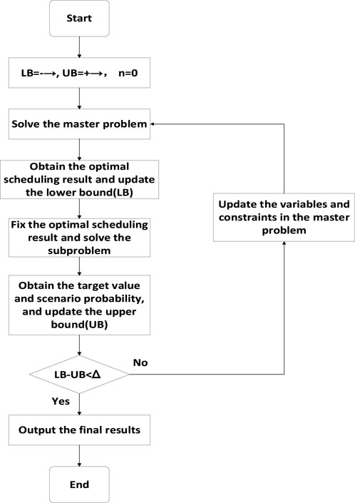
For the two-stage robust optimization model above, this study uses the Column-and- Constraint Generation (C&CG) algorithm to solve it. The C&CG algorithm achieves the optimal solution of the original problem by decomposing it into a master problem and a sub-problem and solving them iteratively in an alternating manner. The main solution logic is illustrated in Figure 2.

Figure 2

Figure 2. Flowchart of the C&CG algorithm.

In the process of solving the master problem using the C&CG algorithm, variables and constraints related to the sub-problem are continuously introduced, allowing for a tighter lower bound of the original objective function value, thereby effectively reducing the number of iterations.

The master problem and sub-problem of the provincial-level dispatch are given by Equations 37 and 38 above. During the iterative process of the C&CG algorithm, the uncertain parameters and their corresponding constraints are dynamically updated. Thus, the formal representations of the master problem and sub-problem should be expressed as follows:

Master Problem Equation 39:

$\begin{array}{l}\min \mathbf{a}\\ s.t.\\ \mathbf{a}\ge \mathbf{cy}\\ \mathbf{Gy}\ge \mathbf{h}-\mathbf{M}{\mathbf{u}}_{\mathbf{k}}-\mathbf{Ex}\\ {\mathbf{G}}_{\mathbf{eq}}\mathbf{y}={\mathbf{h}}_{\mathbf{eq}}-{\mathbf{M}}_{\mathbf{eq}}{\mathbf{u}}_{\mathbf{k}}-{\mathbf{E}}_{\mathbf{eq}}\mathbf{x}\end{array}(39)$

Subproblem Equation 40:

$\begin{array}{l}\text{max min}\mathbf{cy}\\ s.t.\\ \mathbf{Gy}\ge \mathbf{h}-\mathbf{M}{\mathbf{u}}_{\mathbf{k}}-\mathbf{E}{\mathbf{x}}_{\mathbf{value}}\\ {\mathbf{G}}_{\mathbf{eq}}\mathbf{y}={\mathbf{h}}_{\mathbf{eq}}-{\mathbf{M}}_{\mathbf{eq}}{\mathbf{u}}_{\mathbf{k}}-{\mathbf{E}}_{\mathbf{eq}}{\mathbf{x}}_{\mathbf{value}}\end{array}(40)$

fundinWhere ${\mathbf{u}}_{\mathbf{k}}$ denotes the value of the uncertain parameter selected in the kth iteration. In the sub-problem, the variables $\mathbf{x}$ determined by the master problem are treated as constants.

Since the sub-problem is a bilevel problem, this study employs the KKT algorithm to reformulate the inner cost minimization problem into KKT conditions, transforming the bilevel problem into a single-level problem, as shown in Equation 41:

$\begin{array}{l}\max \mathbf{c}\mathbf{y}\\ s.t.\\ \mathbf{Gy}\ge \mathbf{h}-\mathbf{M}{\mathbf{u}}_{\mathbf{k}}-\mathbf{E}{\mathbf{x}}_{\mathbf{value}}\\ {\mathbf{G}}_{\mathbf{eq}}\mathbf{y}={\mathbf{h}}_{\mathbf{eq}}-{\mathbf{M}}_{\mathbf{eq}}{\mathbf{u}}_{\mathbf{k}}-{\mathbf{E}}_{\mathbf{eq}}{\mathbf{x}}_{\mathbf{value}}\\ {\mathbf{G}}^{\mathbf{T}}{\pi }_1+{{\mathbf{G}}_{\mathbf{eq}}}^{\mathbf{T}}{\pi }_2=\mathbf{c}\\ \left(\mathbf{h}-\mathbf{M}{\mathbf{u}}_{\mathbf{k}}-\mathbf{E}{\mathbf{x}}_{\mathbf{value}}-\mathbf{Gy}\right){\pi }_1=\mathbf{0}\\ \left({\mathbf{G}}_{\mathbf{eq}}\mathbf{y}-{\mathbf{h}}_{\mathbf{eq}}+{\mathbf{E}}_{\mathbf{eq}}{\mathbf{x}}_{\mathbf{value}}+{\mathbf{M}}_{\mathbf{eq}}\mathbf{u}\right){\pi }_2=\mathbf{0}\\ \left(\mathbf{c}-{\mathbf{G}}^{\mathbf{T}}{\pi }_1-{\mathbf{G}}_{\mathbf{eq}}^{\mathbf{T}}{\pi }_2\right)\mathbf{y}=\mathbf{0}\\ y\ge 0\\ {\pi }_1\ge 0\end{array}(41)$

It should be noted that the problem contains nonlinear constraints. By using the Big-M method to linearize the constraints, the sub-problem is ultimately converted into a single-level optimization problem, as shown in Equation 42:

$\begin{array}{l}\max \mathbf{c}\mathbf{y}\\ s.t.\\ \mathbf{Gy}\ge \mathbf{h}-\mathbf{M}{\mathbf{u}}_{\mathbf{k}}-\mathbf{E}{\mathbf{x}}_{\mathbf{value}}\\ {\mathbf{G}}_{\mathbf{eq}}\mathbf{y}={\mathbf{h}}_{\mathbf{eq}}-{\mathbf{M}}_{\mathbf{eq}}{\mathbf{u}}_{\mathbf{k}}-{\mathbf{E}}_{\mathbf{eq}}{\mathbf{x}}_{\mathbf{value}}\\ {\mathbf{G}}^{\mathbf{T}}{\pi }_1+{{\mathbf{G}}_{\mathbf{eq}}}^{\mathbf{T}}{\pi }_2=\mathbf{c}\\ {\pi }_1\le M_{\infty }\mathbf{v}\\ \mathbf{Gy}-\mathbf{h}+\mathbf{E}{\mathbf{x}}_{\mathbf{value}}+\mathbf{Mu}\le M_{\infty }\left(1-\mathbf{v}\right)\\ {\pi }_2\le M_{\infty }\mathbf{l}\\ {\mathbf{G}}_{\mathbf{eq}}\mathbf{y}-{\mathbf{h}}_{\mathbf{eq}}+{\mathbf{E}}_{\mathbf{eq}}{\mathbf{x}}_{\mathbf{value}}+{\mathbf{M}}_{\mathbf{eq}}\mathbf{u}\le M_{\infty }\left(1-\mathbf{l}\right)\\ \mathbf{y}\le M_{\infty }\mathbf{w}\\ \mathbf{c}-{\mathbf{G}}^{\mathbf{T}}{\pi }_1-{\mathbf{G}}_{\mathbf{eq}}{\pi }_2\le M_{\infty }\left(1-\mathbf{w}\right)\\ y\ge 0\\ {\pi }_1\ge 0\end{array}(42)$

In the formula, $\mathbf{v},\mathbf{l},\mathbf{w}$ represent auxiliary operators in the Big-M method, all of which are Boolean variables; $M_{\infty }$ is a constant significantly larger than all parameters; ${\pi }_1,{\pi }_2$ denote the Lagrange multipliers in the KKT transformation.

3 Results and discussion

3.1 Regional grid-level dispatch: minimizing the fluctuation of unmet load in each province

Given that the focus of this chapter is on multi-province load peak shaving, a dispatch model for multiple provinces is constructed.

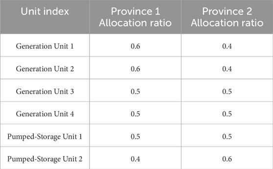
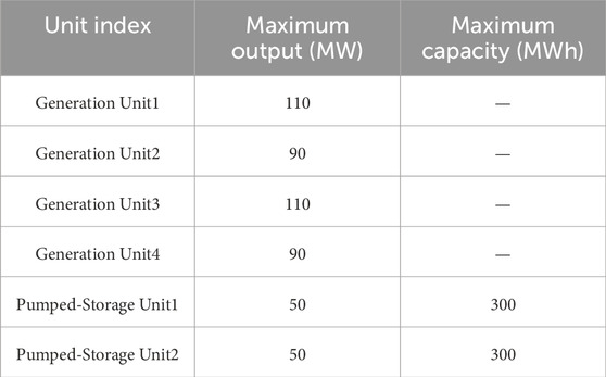
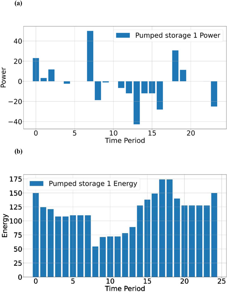
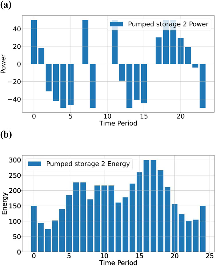
In the inter-provincial dispatch model, four conventional generation units and two pumped-storage units supplying power to two provinces are considered, using 24-period load demand data. The weights for receiving generation output among different provinces are determined based on the ratio of the average load values of each province, and weighting for peak and valley periods is also taken into account.

The average load values of each province and the corresponding weights, generation allocation ratios, and unit data for each generation unit are shown in Tables 1–3.

Table 1

Table 1. Average load values and weights of each province.

Table 2

Table 2. Generation unit allocation ratios.

Table 3

Table 3. Generation unit data.

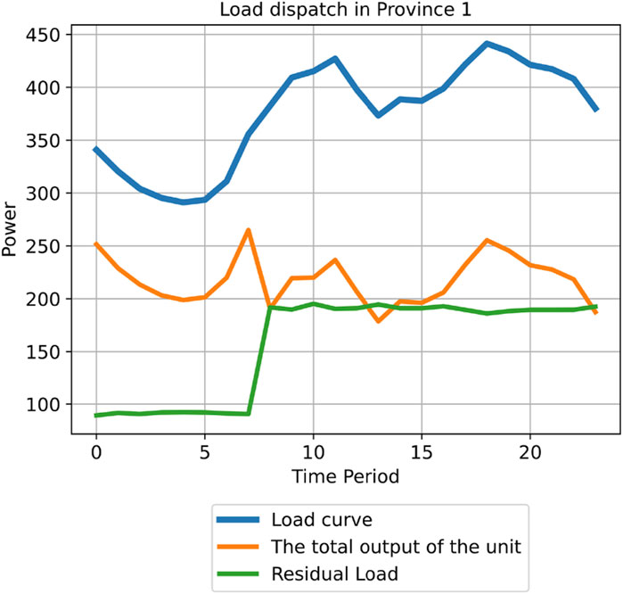
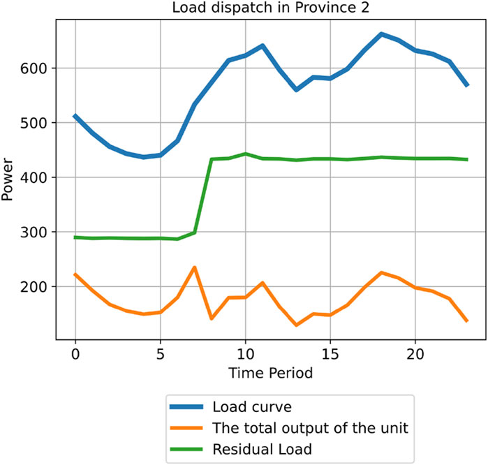
From the data in Table 1, it can be observed that the total maximum output of all units in this study is less than the average load of each province, indicating that the load demand cannot be met in every time period.

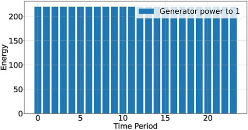
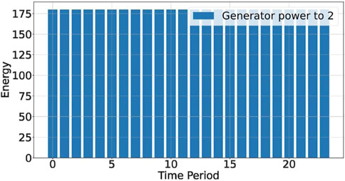
Based on the data from Tables 1 and 3, a model is constructed, and the results are shown in Figures 3–8.

Figure 3

Figure 3. Pumped storage 1 status. (a) Pumped storage 1 Power. (b) Pumped storage 1 Energy.

Figure 4

Figure 4. Pumped storage 2 status. (a) Pumped storage 2 Power. (b) Pumped storage 2 Energy.

Figure 5

Figure 5. Peak shaving results of unmet load in province 1.

Figure 6

Figure 6. Peak shaving results of unmet load in province 2.

Figure 7

Figure 7. Total power received from conventional units in province 1.

Figure 8

Figure 8. Total power received from conventional units in province 2.

As shown in Figures 7, 8, the introduction of the penalty function allows conventional generation units to maintain a high power state even without power balance constraints, indicating that the penalty function construction in this study is effective. Additionally, as seen in Figures 5, 6, the fluctuation degree of the unmet load stabilizes after peak shaving. For Province 1, the valley and peak periods stabilize at 100 MW and 200 MW, respectively, while for Province 2, they stabilize at 300 MW and 440 MW, respectively. This is beneficial for determining the output of backup generation units or the power output from electricity sellers. Stable power delivery can reduce the probability of power system incidents and increase economic benefits.

3.2 Provincial dispatch: robust optimization for uncertainty

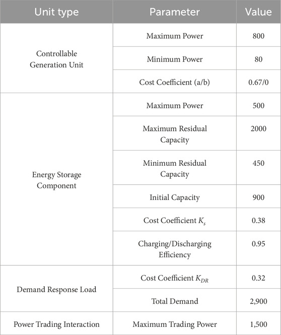
The grid operation parameters are shown in Table 4.

Table 4

Table 4. Grid operation parameters.

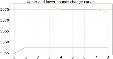
After 24 iterations, the model converged, and the upper and lower bound variation curves are shown in Figure 9.

Figure 9

Figure 9. Upper and lower bound variation curves.

The final results are as follows: the upper bound value is approximately 5,068.342, and the lower bound value is approximately 5,057.569. The result using a standard economic dispatch program is 5,055.049, indicating that the model incurs additional costs to account for extreme scenarios while not deviating significantly from the results of general dispatch methods. This suggests that the model’s solution is reliable.

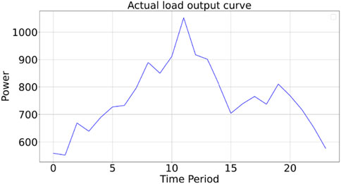
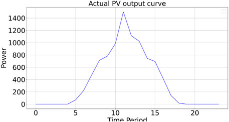
The load demand curve and photovoltaic output curve are shown in Figures 10, 11.

Figure 10

Figure 10. Load demand curve.

Figure 11

Figure 11. Photovoltaic output curve.

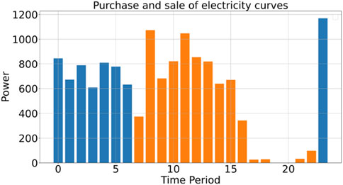
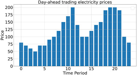
The power trading curve and day-ahead transaction price curve are shown in Figures 12, 13.

Figure 12

Figure 12. Power trading curve.

Figure 13

Figure 13. Day-ahead transaction price curve.

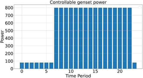
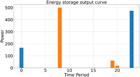
The controllable generation unit output curve and energy storage output curve are presented in Figures 14, 15.

Figure 14

Figure 14. Controllable generation unit output curve.

Figure 15

Figure 15. Energy storage output curve.

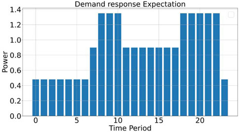
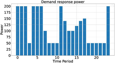
The expected demand response plan and actual demand response load are shown in Figures 16, 17.

Figure 16

Figure 16. Expected demand response plan.

Figure 17

Figure 17. Demand response load curve.

As shown in Figure 11, during periods 1 to 4 and 19 to 24, photovoltaic output is zero, indicating that the load demand is entirely met by controllable generation units, energy storage components, and power purchases. During these periods, when the day-ahead transaction price is lower than the generation cost of controllable units, the output power of controllable units is reduced to the minimum value, as shown in periods 0 to 6 in Figures 12, 14. In the remaining periods, the output power of controllable units is increased to the maximum value to increase the power available for external sales, as seen in periods 7 to 16 and period 20 in Figure 12, or to reduce the power purchase quantity, as shown in periods 17 to 19 and periods 21 and 22 in Figure 12, thereby reducing operational costs.

As observed in Figure 15, under the given pricing mechanism, the energy storage components are charged during periods 6 and 23 and discharged during periods 8, 19, and 20, thereby storing energy during low-price periods and selling it during high-price periods. In Figure 16, the peak electricity price period corresponds to the peak of the expected demand response load plan. By redistributing the electricity demand from periods 18 to 22 to periods 1 to 6 and period 24, the total electricity demand and time-specific electricity constraints are satisfied, reducing the amount of energy that needs to be purchased during peak price periods.

4 Conclusion

This paper primarily investigates the collaborative optimization strategy for regional grid-level and provincial-level dispatch under the influence of renewable energy, focusing on two main issues: peak load shaving in regional grid-level dispatch and uncertainty optimization in provincial-level dispatch.

At the regional grid-level dispatch stage, this paper delves into strategies for effective management of peak shaving and unmet load in a multi-province grid system using pumped-storage units. Traditional peak shaving and valley filling strategies primarily adjust grid operating modes to balance power supply and demand, reducing power consumption during peak periods and increasing power reserves during valley periods. By introducing power variance as the objective function of the optimization problem, this study not only aims to smooth the traditional load curve but also addresses the management of unmet load. Through analyzing the actual power dispatch scenarios between the East China grid and other provincial grids, the paper identifies potential issues of insufficient unit output in cross-regional power trading. To tackle this problem, the study proposes further exploration into the peak shaving demand caused by unmet load and how to manage it through optimized dispatch strategies. To effectively manage load and its residual components, a comprehensive planning method considering both load peak shaving and multi-province dispatch is proposed. By flexibly scheduling energy storage systems such as pumped-storage units, effective management of both load and unmet load can be achieved. This research provides a new perspective and approach for power system operation, enhancing the overall stability and reliability of the grid by addressing unmet load management in addition to traditional peak shaving and valley filling.

At the provincial-level dispatch stage, a two-stage robust optimization model is proposed to minimize economic costs. This model aims to enhance the operational efficiency and reliability of the power system by closely integrating day-ahead dispatch and real-time dispatch. Based on existing modeling methods considering source-load uncertainty, a two-stage robust optimization model is developed. The first stage, day-ahead dispatch, primarily determines the unit status for the following day, while the second stage, real-time dispatch, deals with uncertainties caused by forecast deviations. The model effectively decomposes the complex optimization problem into a master problem and sub-problems. Using the KKT condition algorithm and Column-and-Constraint Generation (C&CG) algorithm, the model can be solved, improving decision accuracy and execution speed. The effectiveness of the proposed two-stage robust optimization model is validated through specific case studies. The results show that this model can maintain power system stability and efficiency by appropriately increasing costs in the face of high uncertainty.

Data availability statement

The raw data supporting the conclusions of this article will be made available by the authors, without undue reservation.

Author contributions

BS: Funding acquisition, Writing – original draft, Conceptualization. KQ: Methodology, Funding acquisition, Writing – review and editing. MW: Writing – review and editing, Conceptualization, Funding acquisition. MZ: Validation, Writing – original draft. KZ: Validation, Writing – review and editing, Writing – original draft. GH: Methodology, Writing – review and editing.

Funding

The author(s) declare that financial support was received for the research and/or publication of this article. This work was supported by the Science and Technology Project of East China Branch of State Grid under Grant No. 529924240008. We would like to extend our sincere gratitude to all project collaborators and contributors for their invaluable insights and support throughout the research.

Conflict of interest

Authors BS, KQ, and MW were employed by East China Branch of State Grid Corporation of China.

The remaining authors declare that the research was conducted in the absence of any commercial or financial relationships that could be construed as a potential conflict of interest.

The authors declare that this study received funding from East China Branch of State Grid. The funder had the following involvement in the study: providing access to power grid operational data and technical expertise.

Generative AI statement

The author(s) declare that no Generative AI was used in the creation of this manuscript.

Publisher’s note

All claims expressed in this article are solely those of the authors and do not necessarily represent those of their affiliated organizations, or those of the publisher, the editors and the reviewers. Any product that may be evaluated in this article, or claim that may be made by its manufacturer, is not guaranteed or endorsed by the publisher.

References

Bendotti, P., Chrétienne, P., Fouilhoux, P., and Pass-Lanneau, A. (2023). The anchor-robust project scheduling problem. Operations Res. 71 (6), 2267–2290. doi:10.1287/opre.2022.2315

CrossRef Full Text | Google Scholar

Büsing, C., and Schmitz, S. (2024). Robust two-stage combinatorial optimization problems under discrete demand uncertainties and consistent selection constraints. Discrete Appl. Math. 347, 187–213. doi:10.1016/j.dam.2023.12.028

CrossRef Full Text | Google Scholar

Cheng, C., Su, C., Wang, P., Shen, J., Lu, J., and Wu, X. (2018). An MILP-based model for short-term peak shaving operation of pumped-storage hydropower plants serving multiple power grids. Energy 163, 722–733. doi:10.1016/j.energy.2018.08.077

CrossRef Full Text | Google Scholar

Chua, K. H., Lim, Y. S., and Morris, S. (2016). Energy storage system for peak shaving. Int. J. Energy Sect. Manag. 10 (1), 3–18. doi:10.1108/ijesm-01-2015-0003

CrossRef Full Text | Google Scholar

Dong, Z., Zhang, Z., Huang, M., Yang, S., Zhu, J., Zhang, M., et al. (2024). Research on day-ahead optimal dispatching of virtual power plants considering the coordinated operation of diverse flexible loads and new energy. Energy 297, 131235. doi:10.1016/j.energy.2024.131235

CrossRef Full Text | Google Scholar

Jin, X., Liu, B., Liao, S., Cheng, C., Zhang, Y., Zhao, Z., et al. (2022). Wasserstein metric-based two-stage distributionally robust optimization model for optimal daily peak shaving dispatch of cascade hydro-plants under renewable energy uncertainties. Energy 260, 125107. doi:10.1016/j.energy.2022.125107

CrossRef Full Text | Google Scholar

Kong, F., Mi, J., and Wang, Y. (2022). A two-stage distributionally robust optimization model for optimizing water-hydrogen complementary operation under multiple uncertainties. J. Clean. Prod. 378, 134538. doi:10.1016/j.jclepro.2022.134538

CrossRef Full Text | Google Scholar

Li, L., Fan, S., Xiao, J., Zhang, Y., Huang, R., and He, G. (2025). Energy management strategy for community prosumers aggregated VPP participation in the ancillary services market based on P2P trading. Appl. Energy 384, 125472. doi:10.1016/j.apenergy.2025.125472

CrossRef Full Text | Google Scholar

Li, L., Fan, S., Xiao, J., Zhou, H., Shen, Y., and He, G. (2024). Fair trading strategy in multi-energy systems considering design optimization and demand response based on consumer psychology. Energy 306, 132393. doi:10.1016/j.energy.2024.132393

CrossRef Full Text | Google Scholar

Liao, S., Xiong, J., Liu, B., Cheng, C., Zhou, B., and Wu, Y. (2024). MILP model for short-term peak shaving of multi-grids using cascade hydropower considering discrete HVDC constraints. Renew. Energy 235, 121341. doi:10.1016/j.renene.2024.121341

CrossRef Full Text | Google Scholar

Liu, Y., and Peng, M. (2024). Research on peak load shifting for hybrid energy system with wind power and energy storage based on situation awareness. J. Energy Storage 82, 110472. doi:10.1016/j.est.2024.110472

CrossRef Full Text | Google Scholar

Luo, B., Liu, X., Chen, Y., Zhou, C., and Long, X. (2024). Short-term peak shaving model of cascade hybrid pumped storage hydropower station retrofitted from conventional hydropower. Int. J. Electr. Power Energy Syst. 162, 110226. doi:10.1016/j.ijepes.2024.110226

CrossRef Full Text | Google Scholar

Meng, Y., Fan, S., Shen, Y., Xiao, J., He, G., and Li, Z. (2023). Transmission and distribution network-constrained large-scale demand response based on locational customer directrix load for accommodating renewable energy. Appl. Energy 350, 121681. doi:10.1016/j.apenergy.2023.121681

CrossRef Full Text | Google Scholar

Niu, T., Yin, H., and Feng, E. (2022). An interval two-stage robust stochastic programming approach for steam power systems design and operation optimization under complex uncertainties. Chem. Eng. Sci. 253, 117533. doi:10.1016/j.ces.2022.117533

CrossRef Full Text | Google Scholar

Shao, Y., Fan, S., Meng, Y., Jia, K., and He, G. (2024). Personalized demand response based on sub-CDL considering energy consumption characteristics of customers. Appl. Energy 374, 123964. doi:10.1016/j.apenergy.2024.123964

CrossRef Full Text | Google Scholar

Uddin, M., Romlie, M. F., Abdullah, M. F., Abd Halim, S., Kwang, T. C., and Chia Kwang, T. (2018). A review on peak load shaving strategies. Renew. Sustain. Energy Rev. 82, 3323–3332. doi:10.1016/j.rser.2017.10.056

CrossRef Full Text | Google Scholar

Wallberg, A., Castellucci, V., Flygare, C., Lind, E., Schultz, E., Mattos, M. M., et al. (2024). Negative correlation peak shaving control in a parking garage in Uppsala, Sweden. Appl. Energy 375, 124082. doi:10.1016/j.apenergy.2024.124082

CrossRef Full Text | Google Scholar

Wang, J., Xu, X., Li, H., and Chen, H. (2022). Two-stage robust optimization of thermal-ESS units scheduling under wind uncertainty. Energy Rep. 8, 1147–1155. doi:10.1016/j.egyr.2022.02.277

CrossRef Full Text | Google Scholar

Wang, J., Zhang, S., Huo, J., Zhou, Y., Li, L., and Han, T. (2021). Dispatch optimization of thermal power unit flexibility transformation under the deep peak shaving demand based on invasive weed optimization. J. Clean. Prod. 315, 128047. doi:10.1016/j.jclepro.2021.128047

CrossRef Full Text | Google Scholar

Wang, M., Xu, X., Fan, S., Yan, Z., Yang, B., and Guan, X. (2025). Multi-period electrical array reconfiguration for multi-PV systems considering net power fluctuation mitigation. J. Mod. Power Syst. Clean Energy 203, 68–80. doi:10.35833/MPCE.2024.000779

CrossRef Full Text | Google Scholar

Wang, M., Xu, X., and Yan, Z. (2023). Online fault diagnosis of PV array considering label errors based on distributionally robust logistic regression. Renew. Energy 203, 68–80. doi:10.1016/j.renene.2022.11.126

CrossRef Full Text | Google Scholar

Yang, S., Fang, J., Zhang, Z., Lv, S., Lin, H., and Ju, L. (2024). Two-stage coordinated optimal dispatching model and benefit allocation strategy for rural new energy microgrid. Energy 292, 130274. doi:10.1016/j.energy.2024.130274

CrossRef Full Text | Google Scholar

Yang, Z., Zheng, H., Du, Y., Guo, L., Xiong, X., and Yao, G. (2023). “Two-stage distributed robust optimization based on multi-discrete scenarios,” in 2023 10th International Forum on Electrical Engineering and Automation (IFEEA), Nanjing, China, 1275–1280.

Google Scholar

Zeng, B., and Zhao, L. (2013). Solving two-stage robust optimization problems using a column-and-constraint generation method. Operations Res. Lett. 41 (5), 457–461. doi:10.1016/j.orl.2013.05.003

CrossRef Full Text | Google Scholar

Zhang, Y., Fan, S., Meng, Y., and He, G. (2025a). Payment and incentive allocation in demand response based on cost causation principle. IEEE Trans. Industry Appl. 1–14. doi:10.1109/tia.2025.3575746

CrossRef Full Text | Google Scholar

Zhang, Y., Meng, Y., Fan, S., Xiao, J., Li, L., and He, G. (2025b). Multi-time scale customer directrix load-based demand response under renewable energy and customer uncertainties. Appl. Energy 383, 125334. doi:10.1016/j.apenergy.2025.125334

CrossRef Full Text | Google Scholar

Zhao, C., and Guan, Y. (2015). Data-driven stochastic unit commitment for integrating wind generation. IEEE Trans. Power Syst. 31 (4), 2587–2596. doi:10.1109/tpwrs.2015.2477311

CrossRef Full Text | Google Scholar

Zhao, H., Liao, S., Ma, X., Fang, Z., Cheng, C., and Zhang, Z. (2024). Short-term peak-shaving scheduling of a hydropower-dominated hydro-wind-solar photovoltaic hybrid system considering a shared multi-energy coupling transmission channel. Appl. Energy 372, 123786. doi:10.1016/j.apenergy.2024.123786

CrossRef Full Text | Google Scholar

Zhu, X., Guo, Y., Li, A., Li, S., Zhang, J., Gu, B., et al. (2024). Two-stage robust optimization of unified power quality conditioner (UPQC) siting and sizing in active distribution networks considering uncertainty of loads and renewable generators. Renew. Energy 224, 120197. doi:10.1016/j.renene.2024.120197

CrossRef Full Text | Google Scholar

Glossary

Sets

$\mathit{T}$ Set of time periods, indexed by $t$

$\mathit{P}$ Set of provinces, indexed by $p$

$\mathit{G}$ Set of generation units, indexed by $g$

Variables and parameters

Regional grid-level variables

${\mathit{P}}_{\mathit{g},\mathit{p},\mathit{t}}$ Output power of unit $g$ to province $p$ at time period $t$

${\mathit{E}}_{\mathit{t}}$ Equivalent stored energy of pumped-storage unit at time period $t$

${\mathit{P}}_{\mathit{t}}^{\mathit{c}\mathit{h}\mathbf{arg}\mathit{e}}$ Pumping power of pumped-storage unit at time period $t$

${\mathit{P}}_{\mathit{t}}^{\mathit{d}\mathit{i}\mathit{s}\mathit{c}\mathit{h}\mathbf{arg}\mathit{e}}$ Generating power of pumped-storage unit at time period $t$

${\mathit{x}}_{\mathit{t}}^{\mathit{c}\mathit{h}\mathbf{arg}\mathit{e}}$ Boolean variable for pumping status at time period $t$

${\mathit{x}}_{\mathit{t}}^{\mathit{d}\mathit{i}\mathit{s}\mathit{c}\mathit{h}\mathbf{arg}\mathit{e}}$ Boolean variable for generating status at time period $t$

Provincial-level variables

${\mathit{P}}_{\mathit{g},\mathit{t}}$ Generation power of controllable unit $g$ at time period $t$

${\mathit{P}}_{\mathit{t}}^{\mathit{c}\mathit{h}}$ Charging power of energy storage at time period $t$

${\mathit{P}}_{\mathit{t}}^{\mathit{d}\mathit{i}\mathit{s}}$ Discharging power of energy storage at time period $t$

${\mathit{u}}_{\mathit{t}}^{\mathit{s}}$ Boolean variable for energy storage charging/discharging state

${\mathit{P}}_{\mathit{t}}^{\mathit{D}\mathit{R}}$ Actual dispatch power of demand response load at time period $t$

${\mathit{P}}_{\mathit{t}}^{\mathit{b}\mathit{u}\mathit{y}}$ Power purchased at time period $t$

${\mathit{P}}_{\mathit{t}}^{\mathit{s}\mathit{e}\mathit{l}\mathit{l}}$ Power sold at time period $t$

${\mathit{u}}_{\mathit{t}}^{\mathit{m}}$ Boolean variable for power trading state (purchase/sale)

${\mathit{P}}_{\mathit{t}}^{\mathit{p}\mathit{v}}$ Actual photovoltaic power at time period $t$

${\mathit{P}}_{\mathit{t}}^{\mathit{L}\mathit{o}\mathit{a}\mathit{d}}$ Actual load power at time period $t$

${\mathit{B}}_{\mathit{t}}^{\mathit{p}\mathit{v}}$ Boolean uncertain parameter for photovoltaic power

${\mathit{B}}_{\mathit{t}}^{\mathit{L}\mathit{o}\mathit{a}\mathit{d}}$ Boolean uncertain parameter for load power

Key parameters

$\mathit{R}{\mathit{U}}_{\mathit{g}}$ Ramp rate limit of thermal power unit $g$

${\mathit{P}}_{\mathit{g}}^{\mathbf{max}}$ Maximum output of unit $g$

${\mathit{P}}_{\mathit{g}}^{\mathbf{min}}$ Minimum generation power of unit $g$

${\mathit{\eta }}_{\mathit{c}\mathit{h}\mathbf{arg}\mathit{e}}$ Efficiency of pumping for pumped-storage station

${\mathit{\eta }}_{\mathit{d}\mathit{i}\mathit{s}\mathit{c}\mathit{h}\mathbf{arg}\mathit{e}}$ Efficiency of power generation for pumped-storage station

${\mathit{E}}^{\mathbf{min}}$ Minimum stored energy of pumped-storage station

${\mathit{E}}^{\mathbf{max}}$ Maximum stored energy of pumped-storage station

${\mathit{R}}_{\mathit{g},\mathit{p}}$ Power transmission ratio of unit $g$ to province $p$

$\mathit{a},\mathit{b}$ Cost coefficients for controllable generation units

${\mathit{K}}_{\mathit{s}}$ Unit charging and discharging cost of energy storage

${\mathit{K}}_{\mathit{D}\mathit{R}}$ Cost coefficient for demand response load

$\mathit{\eta }$ Charging and discharging efficiency of energy storage

${\mathit{D}}_{\mathit{D}\mathit{R}}$ Total electricity demand across all time periods

${\mathit{p}}_{\mathit{t}}$ Day-ahead transaction price at time period $t$