BLformer: a short-term electrical bus load forecasting method based on enhanced Patch-TSTransformer

This study addresses the challenges in short-term electrical bus load forecasting. We propose a novel BLformer framework based on an enhanced Patch-TSTransformer. The framework quantifies the importance of temporal features across three load types and filters key input dimensions to reduce redundant information interference. A sparse attention mechanism is designed to dynamically allocate computational resources, balancing efficiency and robustness. Innovatively, we integrate DCNN into the Patch-TST module, combining the advantages of local feature extraction and global temporal modeling to enhance the learning capability of time-frequency coupling characteristics. Furthermore, a coupled prediction strategy is developed to explore high-accuracy bus load forecasting models that incorporate multiple heterogeneous loads. Experiments demonstrate that BLformer significantly outperforms baseline models in terms of RMSE and MAPE metrics. Notably, the indirect prediction strategy substantially reduces errors compared to direct prediction, validating its effective learning ability for multi-load characteristics.

1 Introduction

With the rapid development of the energy internet and the large-scale integration of renewable energy, the operational environment of power systems has become increasingly complex (Shohan et al., 2022; Rafi et al., 2021). Short-term bus load forecasting, as a core component of power system dispatching, energy trading, and risk control, requires precise capture of the dynamic characteristics and spatiotemporal coupling relationships of multi-source heterogeneous loads (industrial, commercial, and residential). However, the random fluctuations of industrial loads, the seasonal patterns of commercial loads, and the intraday periodic variations of residential loads result in load time series exhibiting nonlinearity, strong time-varying behaviour, and high coupling characteristics. Traditional forecasting methods struggle to account for such complex patterns, necessitating the development of novel and efficient algorithms to support high-accuracy predictions (Mamun et al., 2020; Lai et al., 2020).

With the rapid advancement of artificial intelligence, mainstream methods in the field of short-term load forecasting include neural networks (Ding et al., 2016; Deng et al., 2019), decision trees (Wang et al., 2021; Zhao et al., 2022), extreme learning machines (Li et al., 2016; Chen et al., 2018), deep learning models (Li et al., 2021), and various hybrid forecasting approaches. In the domain of time series prediction, the self-attention mechanism of Transformer (Vaswani et al., 2017) has garnered significant attention due to its exceptional performance in modeling both long- and short-term dependencies. For instance, reference (Yan et al., 2022) proposes a forecasting method based on the Informer model, while Zhang J. et al. (2018) introduces a hybrid approach combining IEMD (Improved Empirical Mode Decomposition), ARIMA (AutoRegressive Integrated Moving Average), and WNN(Wavelet Neural Network). Pang et al. (2024) presents a load forecasting method utilizing bagging random configuration networks, and Hong et al. (2023) develops the CEEMDAN-TGA model, further enhancing prediction accuracy. Additionally, Chu et al. (2022) proposes an improved LSTM(Long Short-Term Memory) network, and Zhang et al. (2020) suggests a short-term load forecasting method that integrates frequency domain decomposition with deep learning. Zhang X. et al. (2018) introduces a novel forecasting framework combining RBM(Restricted Boltzmann Machine) and ENN(Elman neural networks), while Fan et al. (2009) proposes an ensemble neural network for short-term load forecasting. Finally, Wu et al. (2021) presents the Autoformer model, which demonstrates outstanding performance in time series forecasting. These advancements collectively highlight the ongoing evolution and diversification of methodologies aimed at improving the accuracy and reliability of short-term load forecasting.

Existing methods in short-term bus load forecasting are primarily constrained by the following limitations: (1) Feature engineering heavily relies on manual expertise, failing to adaptively identify and select key features, which results in interference from redundant information. (2) Single models struggle to balance the advantages of local feature extraction and global temporal modeling, leading to a pronounced trade-off between computational efficiency and prediction accuracy. Moreover, current models exhibit limited capability in capturing long-term dependencies. (3) There is a lack of effective collaborative mechanisms for multi-source loads, with insufficient consideration of the complementary information inherent in different load types. These issues significantly hinder the practical application and advancement of short-term bus load forecasting methodologies.

In response to the aforementioned challenges, this paper proposes a novel short-term bus load forecasting framework, BLformer, based on an enhanced Patch-TSTransformer. The key contributions of this study are as follows:

(1) Multi-faceted Feature Analysis: We employ a comprehensive approach to quantify the importance of temporal features in industrial, commercial, and residential loads, thereby selecting critical input features to minimize redundancy.

(2) Sparse Attention Mechanism: A sparse attention mechanism is used to enhance the PatchTST model, dynamically allocating computational resources to high-contribution temporal segments, thereby balancing efficiency and robustness.

(3) DCNN-TST Hybrid Architecture: Dilated convolutional layers are embedded into the PatchTST module, combining the local feature extraction capability of DCNN with the global dependency modeling strength of Transformer.

(4) Coupled Prediction Strategy: We explore the differences between direct and indirect prediction strategies incorporating multiple load types, fully leveraging the complementary information among multi-source loads.

Experimental results demonstrate that BLformer significantly outperforms baseline models such as Informer and Autoformer on a regional bus load dataset. Notably, the indirect prediction strategy achieves a substantial reduction in error compared to direct prediction, validating the effectiveness of the proposed framework.

The remainder of this paper is organized as follows: Section 2 provides a detailed analysis of the characteristics of power system bus loads. Section 3 elaborates on the fundamental principles and related technologies of the proposed model. Section 4 describes the structure and prediction workflow of the proposed model. Section 5 validates the effectiveness of the model through case studies and comparative experiments. Finally, Section 6 summarizes the research findings and outlines potential directions for future work.

2 Analysis of electrical bus load characters

As critical nodes in regional power grids, power system buses exhibit load characteristics marked by multi-source heterogeneity. The typical load composition includes three major user groups: industrial, commercial, and residential. The distinct operational patterns of these load types significantly influence the spatiotemporal distribution of bus loads.

2.1 Industrial load characteristics

Industrial users implement refined electricity management based on electricity pricing, resulting in a typical daily load pattern characterized by “low during the day and high at night,” as illustrated in Figure 1. This pattern exhibits a certain periodicity, strongly influenced by production scheduling and pricing policies. During peak pricing periods, production shifts are adjusted to reduce electricity consumption, while full-capacity production is conducted during off-peak periods to optimize cost efficiency. Notably, the load of production-oriented enterprises typically decreases by 40%–60% on weekends and holidays, while continuous production industries (e.g., chemical, steel) experience relatively smoother load fluctuations.

Figure 1

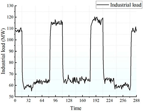
Figure 1. 3-day curve of industrial load.

2.2 Commercial load characteristics

Commercial loads exhibit significant weekday periodicity and peak characteristics, as shown in Figure 2. The typical daily load curve displays a single-peak pattern, with a pronounced drop in load during holidays, often decreasing to 20%–30% of weekday levels during long holidays. Variations in business types lead to differentiated load characteristics: large shopping centers exhibit sharper peak loads compared to office buildings, while the catering industry shows a single-peak pattern during midday.

Figure 2

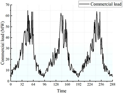
Figure 2. 3-day curve of commercial load.

2.3 Residential load characteristics

Residential loads demonstrate complex multi-peak and time-segmented characteristics with noticeable periodicity, as depicted in Figure 3. During the day, the morning peak is driven by cooking, commuting-related appliances, and heating demands. At midday, the load decreases to 60%–70% of the daily baseline. The evening peak encompasses electricity consumption for cooking, bathing, and entertainment activities. Additionally, residential loads vary significantly across regions, and the emergence of new load types, such as electric vehicles charging in the evening, has led to a noticeable increase in off-peak loads.

Figure 3

Figure 3. 3-day curve of residential load.

2.4 Comprehensive characteristics of bus loads

As illustrated in Figure 4, bus loads exhibit weak periodicity and strong volatility. Specifically, the daily load rate fluctuates dramatically, and the standard deviation of the weekly load rate is also significant. This behaviour stems from two main factors: (1) The superposition of heterogeneous loads diminishes or weakens the original periodic characteristics of multiple load types. (2) The complexity of the power system operating environment, including equipment failures, temporary maintenance, and random changes in user behaviour, leads to sharp fluctuations in the daily load curve. (3) Extreme weather conditions, such as heavy rain, snowstorms, high temperatures, and severe cold, significantly impact power system operations. Furthermore, unexpected events like natural disasters, major social activities, and grid faults can cause abrupt load changes in a short period, further intensifying the volatility of bus loads.

Figure 4

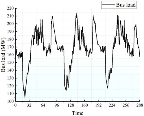
Figure 4. 3-day curve of bus load.

Given the complex characteristics of bus loads described above, traditional forecasting methods that overlook the diverse nature of multi-source loads are inadequate for accurately capturing the underlying patterns of load variations, leading to suboptimal prediction results. Direct prediction approaches fail to sufficiently account for the superposition effects of heterogeneous loads, random disturbances, and the impact of sporadic events. Therefore, in practical power system planning and operation, it is essential to adopt more advanced and precise forecasting methodologies that integrate a comprehensive consideration of these factors. By doing so, the accuracy of bus load forecasting can be significantly improved, enabling more reliable and efficient power system management.

3 Introduction to model principles

3.1 PatchTST model

PatchTST (Patch Time Series Transformer) (Nie et al., 2022) is a time series modeling method based on the Transformer architecture, specifically designed to address long-term dependencies in time series data. It has demonstrated exceptional performance in time series forecasting tasks.

Inspired by the concept of “image patches” in image processing, PatchTST divides time series data into multiple small segments, or “patches,” each representing a segment of the time series. This approach not only reduces the dimensionality of the input sequence, thereby lowering computational complexity, but also preserves the locality of the time series. Simultaneously, it leverages the strengths of Transformer to effectively model long-term dependencies.

The process of PatchTST involves three key steps: First, the original time series data is segmented into fixed-length patches. Second, each patch is encoded to extract its features. Finally, the self-attention mechanism of the Transformer is employed to capture the dependencies among these patches, enabling comprehensive time series modeling and forecasting.

The structure of PatchTST is illustrated in Figure 5.

Figure 5

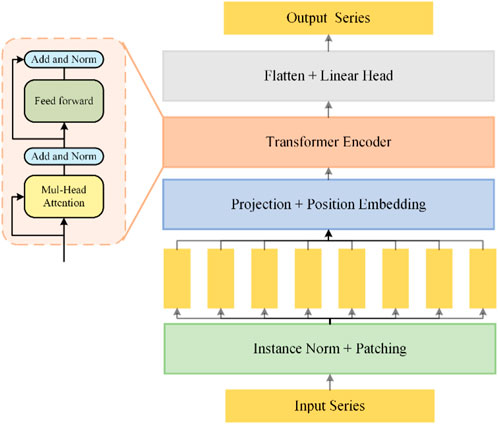
Figure 5. The structure of patchTST.

3.2 Sparse self attention mechanism

Similar to the Transformer, PatchTST employs a multi-head attention mechanism, which introduces challenges such as high computational complexity, information redundancy, difficulties in processing long sequences, and complexities in training and tuning. To address these issues, this paper proposes the use of a sparse attention mechanism to enhance the multi-head attention module in PatchTST.

In the traditional multi-head self-attention mechanism, the inputs are the query vector Q, the key vector K, and the value vector V, which can be expressed as shown in Formula 1:

${\mathbf{Z}}_i=\text{softmax}\left(\frac{{\mathbf{Q}}_i{\mathbf{K}}_i^{\top }}{\sqrt{d_k}}\right){\mathbf{V}}_i(1)$

In the equation: $Q\in R^{L_Q*d}$, $K\in R^{L_K*d}$, $V\in R^{L_V*d}$, d is the input dimension.

The outputs from all attention heads are concatenated and then transformed through a final linear layer to produce the final output as shown in Formula 2:

$\mathbf{Z}=\text{Concat}\left({\mathbf{Z}}_1,\dots ,{\mathbf{Z}}_h\right){\mathbf{W}}_O(2)$

In the equation, ${\mathbf{W}}_O\in {\mathbb{R}}^{h{d}_v\times d_{\text{model}}}$ is the learned projection matrix for the final linear transformation, and h is the number of attention heads.

The dot-product value distribution in the traditional self-attention mechanism follows a long-tailed pattern, indicating that the majority of attention weights contribute minimally, while a small subset of dot products plays a critical role. This observation suggests that it is unnecessary to compute attention scores between all query-key pairs. Instead, computational resources can be focused on the most “important” keys, enabling sparse computation.

The sparsity evaluation formula for the ith query vector Q_i is defined as shown in Formula 3:

$M\left(q_i,K\right)=\ln {\displaystyle \sum _{j=1}^{L_k}}{e}^{\frac{q_i{k}_j^T}{\sqrt{d}}}-\frac{1}{L_k}{\displaystyle \sum _{j=1}^{L_k}}\frac{q_i{k}_j^T}{\sqrt{d}}(3)$

In the formula: The first term, represents the Log-Sum-Exp (LSE) over all key vectors K, and the second term is the arithmetic mean of the dot products between the ith query vector Q_i and all key vectors K_j.

Based on the sparsity evaluation method described above, the final sparse self-attention mechanism can be formulated as shown in Formula 4:

$\text{SparseAttention}\left(Q_i,K,V\right)={\displaystyle \sum _{j\in \text{Top}-\mathrm{k}\left(M\left(Q_i,K\right)\right)}}\text{softmax}\left(\frac{Q_i^T{K}_j}{\sqrt{d_k}}\right)V_j(4)$

where: $\text{Top}-\mathrm{k}\left(M\left(Q_i,K\right)\right)$ selects the top k key vectors with the highest sparsity scores $M\left(Q_i,K\right)$, Q_i is the ith query vector, K_j and V_j are the jth key and value vectors, respectively, d_k is the dimensionality of the key vectors.

This sparse attention mechanism focuses only on the most relevant interactions, significantly reducing computational complexity from O (n²) to O (kn). By dynamically selecting the top k key vectors based on their sparsity scores, the mechanism maintains the model’s ability to capture essential dependencies while improving efficiency and scalability, particularly for long sequences. For the detailed derivation of the specific formula, please refer to reference (Zhou et al., 2021).

3.3 Dilated convolutional neural network (DCNN)

Dilated Convolution (Lei et al., 2019), also known as atrous convolution or expanded convolution, is a convolutional operation that introduces the concept of a dilation rate to standard convolution. By maintaining the same number of kernel parameters, it significantly enlarges the receptive field of the convolution kernel, thereby enhancing the model’s ability to capture long-term temporal dependencies and multi-scale periodic features.

The core idea of dilated convolution lies in the introduction of the dilation rate d, which is defined as follows:

For a convolution kernel of size k and a dilation rate d, the receptive field size R of the dilated convolution is given by Formula 5:

$R=k+\left(k-1\right)\times \left(d-1\right)(5)$

When a convolution kernel W with a dilation rate d is applied to an input sequence x, the computation is defined as shown in Formula 6:

$y\left[i\right]={\displaystyle \sum _{j=0}^{k-1}}W\left[j\right]·x\left[i-j·d\right](6)$

where: x is the input sequence, W represents the convolution kernel parameters, d is the dilation rate, which determines the spacing between kernel elements. By adjusting the dilation rate d, the receptive field of the convolution kernel can be expanded without increasing computational complexity. This enables the model to efficiently capture long-range dependencies and multi-scale features in the input sequence. The schematic diagram is shown in Figure 6.

Figure 6

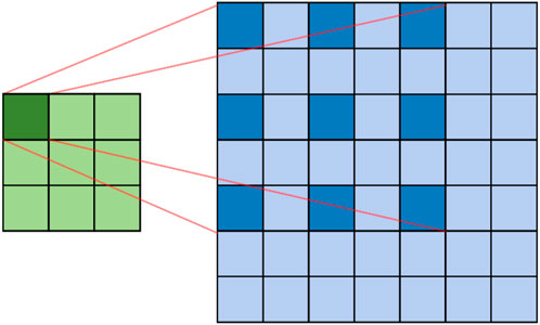
Figure 6. Schematic diagram of dilated convolution.

3.4 Gradient decision tree

LightGBM (Ke et al., 2017) is an efficient machine learning framework based on Gradient Boosting Decision Trees (GBDT). It employs multiple mechanisms for feature selection, including evaluating key features based on feature importance metrics (Split/Gain/SHAP), using histogram binning to reduce computational complexity while retaining effective features, and applying the Gradient-based One-Side Sampling (GOSS) strategy to preserve samples with larger gradients, thereby diminishing the influence of irrelevant features. Additionally, LightGBM adopts a leaf-wise growth strategy, allowing important features to split first, and controls model complexity through parameters such as max_depth and num_leaves to prevent overfitting. L1/L2 regularization further constrains feature weights, and the feature sampling mechanism (feature_fraction) randomly drops a portion of features during training to enhance generalization. By integrating these strategies, LightGBM efficiently and automatically selects important features, improving training speed and prediction performance.

3.5 MIC

The Maximal Information Coefficient (MIC) is a statistical method used to measure the nonlinear correlation between two variables. Its core idea is to quantify the relationship between features using normalized maximal mutual information. The MIC is defined as shown in Formula 7:

$I\left(X,Y\right)={\displaystyle \sum _{x\in X}}{\displaystyle \sum _{y\in Y}}P\left(x,y\right)\log \frac{P\left(x,y\right)}{P\left(x\right)P\left(y\right)}(7)$

In the formula, $p\left(x,y\right)$ is the joint probability distribution, $P\left(x\right)$ and $P\left(y\right)$ is the marginal probability distribution.

4 Short-term bus load forecasting method based on enhanced Patch-TSTransformer

4.1 Multiple feature selection mechanism

We propose a multi-faceted feature selection mechanism that leverages both LightGBM and MIC to evaluate the association between industrial, commercial, and residential loads and other features. This approach enables complementary screening of multi-source heterogeneous data, offering advantages over single-method feature selection:

On one hand, LightGBM, with its gradient-boosting tree architecture, constructs predictive models for each load type and identifies features with significant predictive power through feature importance scores. This allows for the extraction of features that have a strong influence on load forecasting.

On the other hand, the Maximal Information Coefficient (MIC) quantifies the nonlinear statistical dependence between features and loads, avoiding the limitations of model assumptions and capturing potential complex relationships that might otherwise be overlooked.

By integrating the results from both methods, we retain core features that exhibit high predictive value or strong statistical associations across different load types. This dual approach effectively reduces the interference of redundant information while balancing model generalization and interpretability.

4.2 Coupling prediction strategy

We propose a novel coupling prediction strategy based on multi-source heterogeneous characteristics, specifically optimized for bus load forecasting scenarios. This method begins by constructing distinct prediction models for industrial, commercial, and residential sub-loads, each tailored to capture their unique features. After precise modeling of each component, the predictions are dynamically weighted and integrated. Compared to directly forecasting the total bus load as a whole, this approach effectively addresses the limitations of traditional aggregate forecasting methods, which often overlook the heterogeneity of different load types.

4.3 The model structure of BLformer

To improve the accuracy of short-term bus load forecasting, this paper proposes the BLformer model, as illustrated in Figure 7.

Layer 1: LightGBM + MIC Layer

Figure 7

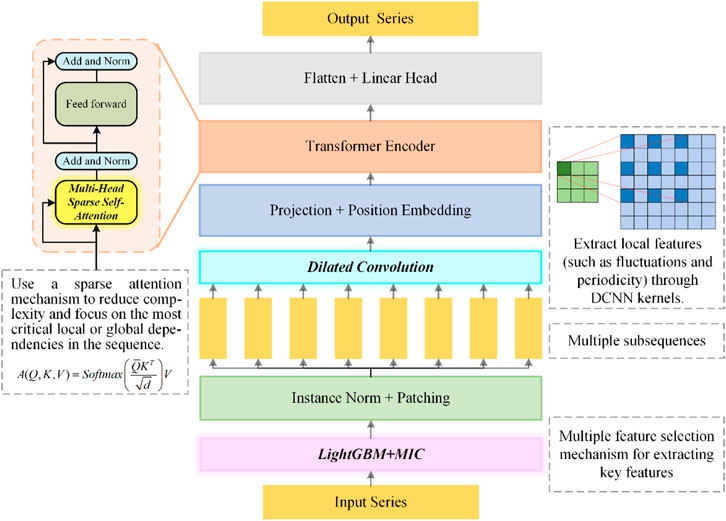
Figure 7. Model structure of BLformer.

This layer employs LightGBM and MIC algorithms to explore the nonlinear relationships between bus loads and external features such as meteorological parameters (e.g., temperature, humidity) and holidays. It identifies the subset of features that contribute most significantly to load forecasting, effectively reducing input dimensionality while retaining key drivers of load variations. This step provides high-information-density time series features as input for subsequent deep learning modules.

Layer 2: Instance Norm + Patching Layer

Instance normalization (Instance Norm) performs local standardization on bus loads to account for their time-varying characteristics and eliminate scale differences. Patching divides continuous time series into fixed-length windows, preserving local patterns of short-term load fluctuations while laying the foundation for multi-scale time series feature extraction in subsequent layers. This block-based strategy balances local sensitivity and global modeling capabilities.

Layer 3: Dilated Convolution Layer

By adjusting the dilation rate of the convolution kernel, this layer captures long-term periodic patterns (e.g., annual/quarterly load trends) and cross-temporal correlations (e.g., differences between holiday and weekday patterns) at a low computational cost. Compared to standard convolutions, the sparse connectivity of dilated convolutions significantly enhances the efficiency of time series feature propagation, making it particularly suitable for scenarios with long-term fluctuations (e.g., seasonal electricity usage habits) while avoiding overfitting risks associated with fully connected layers.

Layer 4: Projection + Position Embedding Layer

The projection layer compresses multi-channel patch features into a unified space, eliminating dimensional differences between channels. Position embedding assigns a time-sensitive global identifier to each patch, explicitly incorporating absolute time information (e.g., day of the week, season) and relative temporal relationships (e.g., time intervals between adjacent patches).

Layer 5: Multi-head Sparse Attention Transformer Encoder

The multi-head attention mechanism computes correlations across different time scales in parallel, while the sparsity strategy reduces computational complexity by limiting the attention window. The multi-layer Transformer encoder iteratively refines implicit temporal patterns through self-attention, making it particularly effective at capturing complex nonlinear temporal dependencies in bus loads. The output is a temporal representation matrix.

Layer 6: Flatten + Linear Head Layer

The flatten operation transforms high-dimensional feature maps into a one-dimensional vector, which is then fed into a linear output layer to map the feature space to the prediction space, generating the final forecast results.

4.4 Prediction process

The proposed bus load forecasting model follows a systematic workflow of “data preprocessing—feature selection—model training and optimization—prediction result reconstruction,” as illustrated in Figure 8. The specific steps are as follows:

Step 1. Data Preprocessing

Figure 8

Figure 8. Prediction process diagram.

The original bus load data and meteorological data serve as critical input sources for the model, and their quality directly impacts the accuracy and reliability of the forecasting results. To ensure high-quality data, the following preprocessing steps are performed:

Outlier Removal: The Interquartile Range (IQR) method is used to detect and remove outliers in both bus load and meteorological data that deviate from the normal range.

Missing Value Imputation: Linear interpolation based on time series characteristics is employed to efficiently fill in missing values in the data.

Step 2. Dataset Division and Feature Selection

The preprocessed dataset is divided into training, validation, and test sets in a 7:2:1 ratio. The training set is used for model training. The validation set is used for hyperparameter tuning and model performance evaluation. The test set is used for final model performance validation.

Feature selection is then performed: LightGBM is used to calculate the importance scores of input features. The Maximal Information Coefficient (MIC) algorithm is applied to assess feature redundancy. Based on the combined results of LightGBM and MIC, features with lower contribution rankings are removed to reduce model complexity and improve prediction efficiency and generalization ability.

Step 3. Model Training and Optimization

The BLformer model is used to construct separate prediction sub-models for industrial, commercial, and residential loads. Grid Search is employed to optimize key hyperparameters (e.g., learning rate). The Root Mean Square Error (RMSE) on the validation set is used as the evaluation metric to select the optimal hyperparameter combination, ensuring a balance between prediction accuracy and computational efficiency.

Step 4. Prediction Result Reconstruction and Fusion

The outputs of the BLformer model for industrial, commercial, and residential loads are reconstructed and fused: A weighted average method is used for preliminary fusion of the three load predictions. The weights are determined based on the historical proportion of each load type in the total bus load. The adjusted prediction results are denormalized and output, yielding high-accuracy bus load forecasts.

5 Examples and experimental analysis

5.1 Dataset description and model development environment

This study is based on real operational data from a specific region in 2020, with a sampling frequency of 15 min. The dataset encompasses multi-dimensional load information, including industrial, commercial, residential, and bus load data. Additionally, key meteorological parameters such as temperature, air pressure, relative humidity, rainfall, and solar radiation intensity were collected, providing comprehensive data support for the construction of the load forecasting model.

For model development, Python 3.10 was used as the programming language, and the prediction model was built on the PyTorch deep learning framework. To ensure efficient and reliable model training, the experimental platform was equipped with high-performance computing hardware: a 14th-generation Intel Core i7 processor, an NVIDIA GeForce RTX 4090 graphics card, and 128 GB of RAM, providing robust computational power for training and optimizing the deep learning model.

5.2 Prediction evaluation metrics

To assess the prediction accuracy of the model, three widely recognized statistical metrics were selected: Mean Absolute Error (MAE), Root Mean Square Error (RMSE), and Mean Absolute Percentage Error (MAPE). The definitions of these metrics are as shown in Formulas 8–10:

$\text{MAE}=\frac{1}{n}{\displaystyle \sum _{i=1}^n}\left|y_i-{\widehat{y}}_i\right|(8)$

$\text{RMSE}=\sqrt{\frac{1}{n}{\displaystyle \sum _{i=1}^n}{\left(y_i-{\widehat{y}}_i\right)}^2}(9)$

$\text{MAPE}=\frac{100\%}{n}{\displaystyle \sum _{i=1}^n}\left|\frac{y_i-{\widehat{y}}_i}{y_i}\right|(10)$

In the formula, $y_i$ is the actual value, ${\widehat{y}}_i$ is the predicted value, and n is the sample size.

5.3 Feature contribution analysis

Based on expert knowledge, the initial input features were selected, including historical load information, weather data, and calendar rules as shown in Table 1.

1. Load Information: Historical load data from the previous 4 h for industrial, commercial, and residential loads.

2. Weather Data: Temperature, air pressure, humidity, rainfall, and solar irradiance.

3. Calendar Rules: Hour of the day, day of the week, season, and holiday information.

Table 1

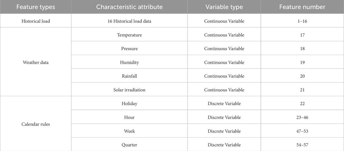
Table 1. Type and number of features.

To avoid mutual influence between continuous data, calendar rule information was discretized using one-hot encoding. This ensures that each categorical feature is represented independently, enhancing the model’s ability to capture their distinct effects.

To explore the dominant factors affecting load forecasting accuracy, this study employs both LightGBM and MIC algorithms to analyze the contribution of load and weather features. The results are shown in Figures 9–14. The analysis reveals that the two algorithms exhibit different sensitivities to load and weather features, indicating that combining multiple algorithms for feature importance evaluation provides a more comprehensive understanding of feature contributions, thereby improving prediction accuracy.

Figure 9

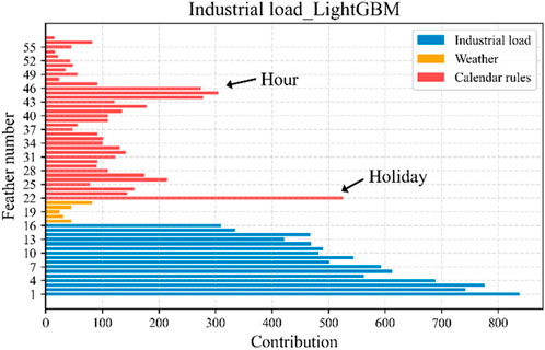
Figure 9. Correlation results of industrial load LightGBM.

Figure 10

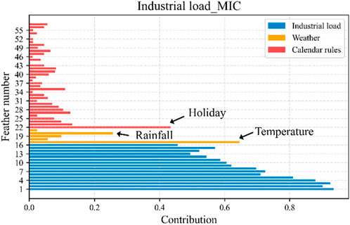
Figure 10. Correlation results of industrial load MIC.

Figure 11

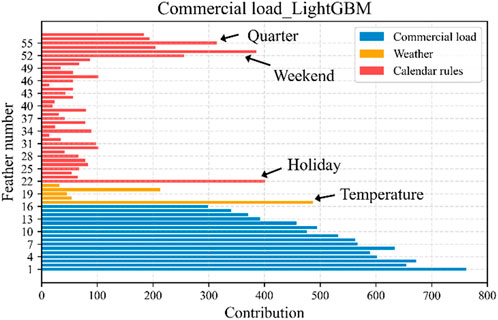
Figure 11. Correlation results of commercial load LightGBM.

Figure 12

Figure 12. Correlation results of commercial load MIC.

Figure 13

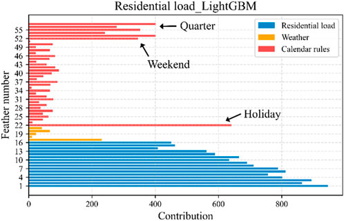
Figure 13. Correlation results of residential load LightGBM.

Figure 14

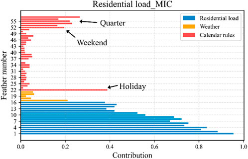
Figure 14. Correlation results of residential load MIC.

For industrial load, both algorithms show significant correlations with historical industrial load and holiday information. Notably, LightGBM is more sensitive to certain hour-related features, while MIC demonstrates stronger sensitivity to rainfall and temperature, particularly showing a significant correlation with temperature. Given the practical impact of rainfall and high temperatures on factory production, the industrial load prediction model incorporates historical industrial load, temperature, rainfall, and holiday features based on the combined evaluation results of the two algorithms.

For commercial load, both algorithms indicate that historical commercial load, holiday information, temperature, and weekend information have important influences. LightGBM shows some sensitivity to seasonal information, while MIC does not exhibit similar characteristics. Considering the limited practical impact of seasonal changes on commercial activities, the commercial load prediction model includes historical commercial load, temperature, holiday, and weekend features based on the combined evaluation results.

For residential load, the analysis results of the two algorithms are highly consistent, both indicating significant correlations with historical residential load, holidays, weekends, and seasonal information. Given the substantial influence of these factors on residential behaviour patterns, the residential load prediction model incorporates historical residential load, holidays, weekends, and seasonal features based on the combined evaluation results.

The final input features for the three load models are summarized in Table 2.

Table 2

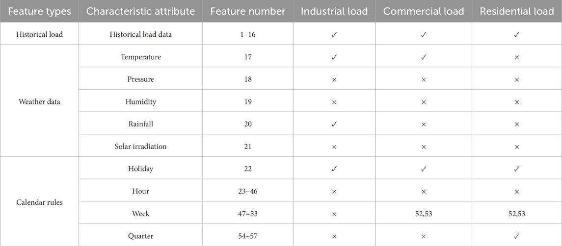
Table 2. Feature input table.

5.4 Model parameter settings

To achieve the best prediction performance, this study optimized the hyperparameters of the model through grid search algorithm, using root mean square error (RMSE) as the evaluation index. The final determined parameter combinations are shown in Table 3.

Table 3

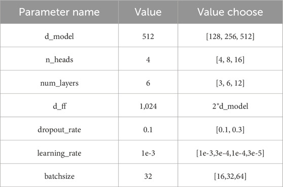
Table 3. Parameter selection and optimization range.

5.5 Analysis of model prediction performance

To validate the predictive performance of the BLformer model, this study selects three mainstream time series forecasting models—Informer, Autoformer, and Fedformer—as benchmark comparisons. The experiments adopt a coupled prediction paradigm, where industrial, commercial, and residential loads are independently predicted, and the bus load prediction results are obtained through load superposition. All comparative models undergo hyperparameter optimization, and the prediction duration is uniformly set to a 24-h rolling forecast.

As visually compared in Figure 15, the BLformer’s prediction curve is the closest to the true value distribution, outperforming the benchmark models in both trend tracking and peak-valley feature capturing. Its prediction trajectory synchronizes well with the true curve, demonstrating excellent temporal following capability. In contrast, Informer and Autoformer exhibit significant prediction deviations during abrupt load changes, while Fedformer, although improved in overall accuracy, still suffers from phase shift issues. Specifically, the baseline models show notably larger prediction errors in steep load rise/fall intervals compared to the proposed method.

Figure 15

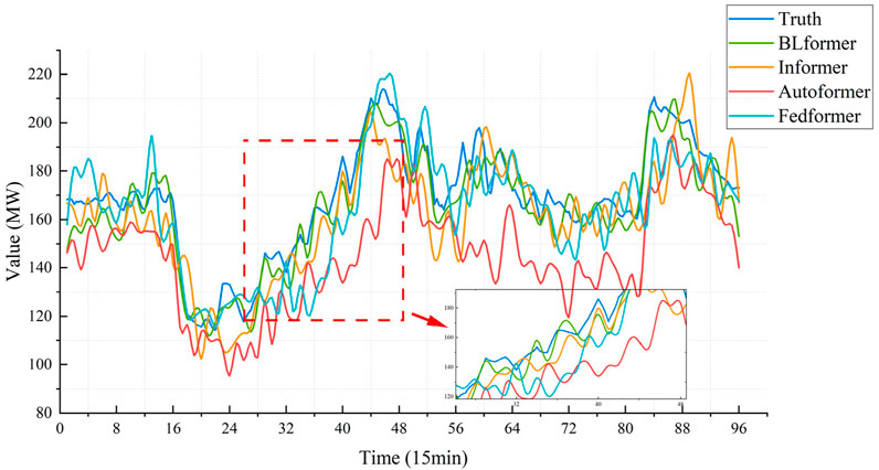
Figure 15. Prediction curve.

Furthermore, based on the model prediction accuracy comparison results shown in Table 4, the proposed BLformer model demonstrates significant advantages in forecasting industrial, commercial, residential, and bus loads. Specifically, compared to mainstream time series forecasting models such as Informer, Autoformer, and Fedformer, BLformer achieves the best performance across three key evaluation metrics (RMSE, MAE, MAPE).

Table 4

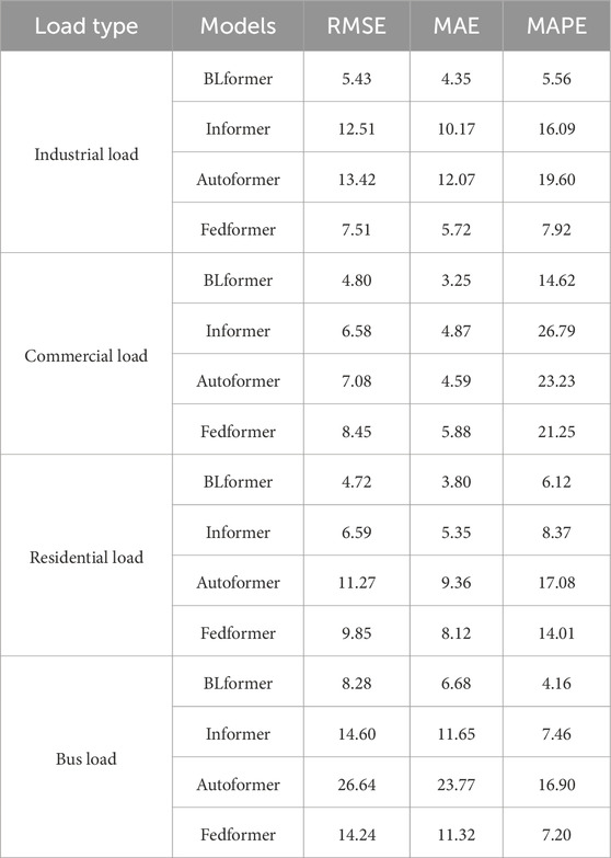
Table 4. Performance comparison of load forecasting models (units: RMSE/MW, MAE/MW, MAPE/%).

For example, in industrial load forecasting, BLformer’s RMSE (5.43), MAE (4.35), and MAPE (5.56%) are on average 27.6%, 23.9%, and 29.8% lower, respectively, than those of the second-best model, Fedformer. This validates the effectiveness of BLformer in capturing complex industrial load patterns.

5.6 Ablation experiment

To further validate the effectiveness of each module in the BLformer model, we conducted ablation experiments. The results, as shown in Table 5, demonstrate that the synergistic integration of modules in BLformer achieves simultaneous improvements in prediction accuracy and computational efficiency. Compared to the baseline model, PatchTST, the full version of BLformer shows significant enhancements across all three metrics: RMSE (8.28 vs. 15.61), MAE (6.68 vs. 11.05), and MAPE (4.16% vs. 6.01%), representing improvements of 46.9%, 39.5%, and 30.8%, respectively. These results confirm the effectiveness of the module design.

Table 5

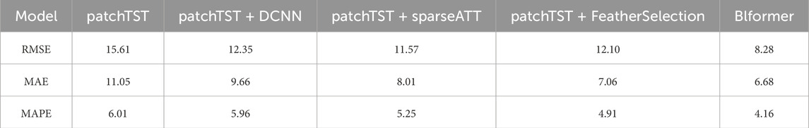
Table 5. Model prediction accuracy table.

Sparse Attention Module (sparseATT): This module significantly reduces computational complexity. In bus load forecasting, the single-module version reduces training time by 9.0% (38.5 vs. 42.3 min) while lowering RMSE by 25.9% (11.57 vs. 15.61), demonstrating its efficiency in modeling long-term dependencies.

Feature Selection Module (FeatherSelection): This module exhibits excellent noise suppression capabilities. In bus load forecasting, it improves the MAE metric by 36.2% (7.06 vs. 11.05) and reduces redundant feature computations by 30% through dynamic pruning.

Dilated Convolution Module (DCNN): This module effectively captures abrupt load changes. However, its standalone use increases training time by 11.3% (47.1 vs. 42.3 min), highlighting the necessity of module co-optimization.

Integrated Performance: When all modules are integrated, BLformer achieves a training time of 40.2 min, which is 4.9% shorter than the baseline model and 14.6% faster than the version using only DCNN. This efficiency gain stems from: sparseATT reducing the spatial complexity of traditional attention mechanisms. FeatherSelection decreasing forward propagation computations through adaptive feature pruning.

The experimental results demonstrate that BLformer, through the organic integration of sparse attention mechanisms, dynamic feature selection, and dilated convolutions, achieves precise modeling of complex load characteristics while maintaining model lightweightness. This provides an efficient and effective solution for real-world power system forecasting tasks.

5.7 Comparison between direct prediction and indirect prediction

This section validates the performance advantages of the coupled prediction method through experimental analysis. First, Figures 16–19 illustrate the forecasting results of the coupled prediction model for industrial, commercial, and residential loads. Then, Figure 19 presents a comparative analysis between the coupled prediction approach and direct bus load prediction. The experimental results demonstrate that coupled prediction significantly outperforms direct prediction in both accuracy and stability. This improvement is primarily attributed to the ability of the coupled prediction method to fully account for the interactions among industrial, commercial, and residential loads, as well as the distinct characteristics of each load type. By establishing a coupling mechanism that captures the inherent correlations between different load types, the proposed method effectively enhances overall forecasting performance.

Figure 16

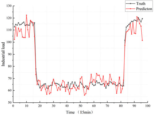
Figure 16. Industrial load forecast results.

Figure 17

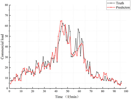
Figure 17. Commercial load forecast results.

Figure 18

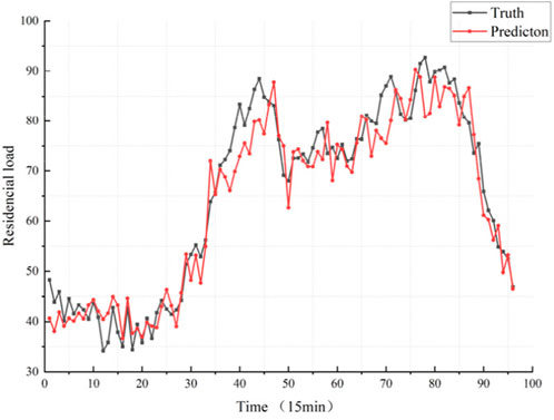
Figure 18. Residential load forecast results.

Figure 19

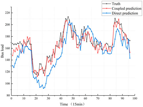
Figure 19. Bus load forecast results.

6 Conclusion

This study proposes a short-term bus load forecasting framework based on an enhanced Patch-TSTransformer, termed BLformer. Through theoretical analysis and experimental validation, the following conclusions are drawn:

1. The innovatively designed multi-feature analysis mechanism effectively identifies and selects key input features, significantly improving prediction accuracy while reducing feature redundancy.

2. The proposed sparse attention mechanism, combined with the DCNN-TST hybrid architecture, optimally allocates computational resources. This design autonomously identifies and focuses on high-contribution temporal segments, enhancing prediction robustness while maintaining model efficiency.

3. Compared to traditional direct bus load forecasting methods, the coupled forecasting strategy introduced in this study significantly improves forecasting accuracy by capturing the interaction relationships among multiple load types.

Experimental results demonstrate that BLformer outperforms mainstream baseline models such as Informer and Autoformer on regional bus load datasets. Furthermore, the indirect prediction strategy substantially reduces forecasting errors compared to direct prediction, fully validating the effectiveness and practical applicability of the proposed method.

Data availability statement

The data analyzed in this study is subject to the following licenses/restrictions: Data is confidential. Requests to access these datasets should be directed to the corresponding author.

Author contributions

HL: Writing – original draft. QC: Writing – original draft, Methodology. DZ: Project administration, Writing – review and editing. HW: Writing – original draft, Investigation. XZ: Supervision, Writing – original draft, Validation. ZZ: Writing – review and editing, Formal Analysis. LF: Investigation, Writing – original draft, Methodology. WW: Supervision, Writing – review and editing, Software. SC: Writing – original draft, Visualization.

Funding

The author(s) declare that financial support was received for the research and/or publication of this article. This research is supported by State Grid Beijing Electric Power Company Science and Technology Project: Research and application of short-term and ultra-short-term load accurate forecasting technology for large urban power grids (520223240004).

Conflict of interest

Authors HL, DZ, XZ, and LF were employed by State Grid Beijing Electric Power Company. Author SC was employed by Beijing Tsingsoft Technology Co., Ltd.

The remaining authors declare that the research was conducted in the absence of any commercial or financial relationships that could be construed as a potential conflict of interest.

The authors declare that this study received funding from State Grid Beijing Electric Power Company. The funder had the following involvement in the study, such as providing technical advice, collecting field data, approving manuscript content.

Generative AI statement

The author(s) declare that no Generative AI was used in the creation of this manuscript.

Publisher’s note

All claims expressed in this article are solely those of the authors and do not necessarily represent those of their affiliated organizations, or those of the publisher, the editors and the reviewers. Any product that may be evaluated in this article, or claim that may be made by its manufacturer, is not guaranteed or endorsed by the publisher.

References

Chen, Y., Kloft, M., Yang, Y., Li, C., and Li, L. (2018). Mixed kernel based extreme learning machine for electric load forecasting. Neurocomputing 312, 90–106. doi:10.1016/j.neucom.2018.05.068

CrossRef Full Text | Google Scholar

Chu, X., Gao, Y., Qiu, Y., Li, M., Fan, H., Shi, M., et al. (2022). “Short-term load forecast using improved long-short term memory network,” in 2022 IEEE 5th International Electrical and Energy Conference (CIEEC), 1228–1233. doi:10.1109/CIEEC54735.2022.9845931

CrossRef Full Text | Google Scholar

Deng, Z., Wang, B., Xu, Y., Xu, T., Liu, C., and Zhu, Z. (2019). Multi-scale convolutional neural network with time-cognition for multi-step short-term load forecasting. IEEE Access 7, 88058–88071. doi:10.1109/ACCESS.2019.2926137

CrossRef Full Text | Google Scholar

Ding, N., Benoit, C., Foggia, G., Bésanger, Y., and Wurtz, F. (2016). Neural network-based model design for short-term load forecast in distribution systems. IEEE Trans. Power Syst. 31, 72–81. doi:10.1109/TPWRS.2015.2390132

CrossRef Full Text | Google Scholar

Fan, S., Chen, L., and Lee, W. (2009). Short-term load forecasting using comprehensive combination based on multimeteorological information. IEEE Trans. Industry Appl. 45, 1460–1466. doi:10.1109/TIA.2009.2023571

CrossRef Full Text | Google Scholar

Hong, Y., Wang, D., Su, J., Ren, M., Xu, W., Wei, Y., et al. (2023). Short-term power load forecasting in three stages based on CEEMDAN-TGA model. Sustainability 15, 11123. doi:10.3390/su151411123

CrossRef Full Text | Google Scholar

Ke, G., Meng, Q., Finley, T., Wang, T., Chen, W., Ma, W., et al. (2017). Lightgbm: a highly efficient gradient boosting decision tree. Adv. neural Inf. Process. Syst., 30. Available online at: https://scholar.google.com/scholar?q=Lightgbm:+A+highly+efficient+gradient+boosting+decision+tree&hl=zh-CN&as_sdt=0&as_vis=1&oi=scholart.

Google Scholar

Lai, C., Mo, Z., Wang, T., Yuan, H., Ng, W., and Lai, L. (2020). Load forecasting based on deep neural network and historical data augmentation. IET Generation, Transm. & Distribution 14, 5927–5934. doi:10.1049/iet-gtd.2020.0842

CrossRef Full Text | Google Scholar

Lei, X., Pan, H., and Huang, X. (2019). A dilated CNN model for image classification. IEEE Access 7, 124087–124095. doi:10.1109/ACCESS.2019.2927169

CrossRef Full Text | Google Scholar

Li, S., Goel, L., and Wang, P. (2016). An ensemble approach for short-term load forecasting by extreme learning machine. Appl. Energy 170, 22–29. doi:10.1016/J.APENERGY.2016.02.114

CrossRef Full Text | Google Scholar

Li, Z., Li, Y., Liu, Y., Wang, P., Lu, R., and Gooi, H. (2021). Deep learning based densely connected network for load forecasting. IEEE Trans. Power Syst. 36, 2829–2840. doi:10.1109/TPWRS.2020.3048359

CrossRef Full Text | Google Scholar

Mamun, A., Sohel, M., Mohammad, N., Sunny, M., Dipta, D., and Hossain, E. (2020). A comprehensive review of the load forecasting techniques using single and hybrid predictive models. IEEE Access 8, 134911–134939. doi:10.1109/access.2020.3010702

CrossRef Full Text | Google Scholar

Nie, Y., Nguyen, N. H., Sinthong, P., and Kalagnanam, J. (2022). A time series is worth 64 words: long-term forecasting with transformers. arXiv Prepr. arXiv:2211.14730. Available online at: https://arxiv.org/abs/2211.14730

Google Scholar

Pang, X., Sun, W., Li, H., Liu, W., and Luan, C. (2024). Short-term power load forecasting method based on Bagging-stochastic configuration networks. PLOS ONE 19, e0300229. doi:10.1371/journal.pone.0300229

PubMed Abstract | CrossRef Full Text | Google Scholar

Rafi, S., Nahid-Al-Masood, , Deeba, S., and Hossain, E. (2021). A short-term load forecasting method using integrated CNN and LSTM network. IEEE Access 9, 32436–32448. doi:10.1109/ACCESS.2021.3060654

CrossRef Full Text | Google Scholar

Shohan, M., Faruque, M., and Foo, S. (2022). Forecasting of electric load using a hybrid LSTM-neural prophet model. Energies 15, 2158. doi:10.3390/en15062158

CrossRef Full Text | Google Scholar

Vaswani, A., Shazeer, N., Parmar, N., Uszkoreit, J., Jones, L., Gomez, A. N., et al. (2017). “Attention is all you need,” in Proceedings of the 31st international conference on neural information processing systems (NIPS'17) (Red Hook, NY, USA: Curran Associates Inc.), 6000–6010.

Google Scholar

Wang, Y., Sun, S., Chen, X., Zeng, X., Kong, Y., Chen, J., et al. (2021). Short-term load forecasting of industrial customers based on SVMD and XGBoost. Int. J. Electr. Power & Energy Syst. 129, 106830. doi:10.1016/J.IJEPES.2021.106830

CrossRef Full Text | Google Scholar

Wu, H., Xu, J., Wang, J., and Long, M. (2021). Autoformer: decomposition Transformers with auto-correlation for long-term series forecasting. Adv. Neural Inf. Process. Syst. 34 22419–22430. Available online at: https://arxiv.org/abs/2106.13008

Google Scholar

Yan, Y., Li, W., Su, S., Bai, H., Yang, Y., Pan, S., et al. (2022). Decentralized wind power forecasting method based on informer. Recent Adv. Electr. & Electron. Eng. 15 (Issue 8), 679–687. doi:10.2174/2352096515666220818122603

CrossRef Full Text | Google Scholar

Zhang, J., Wei, Y., Li, D., Tan, Z., and Zhou, J. (2018a). Short term electricity load forecasting using a hybrid model. Energy 158, 774–781. doi:10.1016/J.ENERGY.2018.06.012

CrossRef Full Text | Google Scholar

Zhang, Q. Y., Li, G. J., Ding, J., and Ma, J. (2020). Short-term load forecasting based on frequency domain decomposition and deep learning. Math. Problems Eng. 2020, 1–9. doi:10.1155/2020/7240320

CrossRef Full Text | Google Scholar

Zhang, X., Wang, R., Tao, Z., Liu, Y., and Zha, Y. (2018b). Short-term load forecasting using a novel deep learning framework. Energies 11, 1554. doi:10.3390/EN11061554

CrossRef Full Text | Google Scholar

Zhao, X., Li, Q., Xue, W., Zhao, Y., Zhao, H., and Guo, S. (2022). Research on ultra-short-term load forecasting based on real-time electricity price and window-based XGBoost model. Energies 15, 7367. doi:10.3390/en15197367

CrossRef Full Text | Google Scholar

Zhou, H., Zhang, S., Peng, J., Li, J., Xiong, H., and Zhang, W. (2021). Informer: beyond efficient Transformer for long sequence time-series forecasting. Proc. AAAI Conf. Artif. Intell. 35 (12), 11106–11115. doi:10.1609/aaai.v35i12.17325

CrossRef Full Text | Google Scholar