Earthworm optimization algorithm for extracting parameters for solar cells and photovoltaic modules

In this paper, we deal with the use of the earthworm optimization algorithm (EOA) in foraging to estimate and extract the intrinsic electrical parameters of single-, double-, and triple-diode solar cells and photovoltaic modules across different technologies. This method was chosen to address the challenges associated with the nonlinear behavior, complexity, and mathematical modeling of solar cells and photovoltaic modules (PVMs). The objective function is modified to minimize the absolute errors between experimental and simulated current values. The EOA in foraging is applied to three different case studies: the RTC France solar cell, the Photowatt-PWP 201 PV module, and the Schutten Solar STM6-40/36 monocrystalline module, under varying solar irradiance and ambient temperature conditions. The goal is to identify the parameters of the single-diode (SD), double-diode (DD), and triple-diode (TD) models. In addition, the proposed objective function is computed based on the current–voltage (I–V) characteristic curve. The extracted parameters for each case study are used to reconstruct the I–V and power–voltage (P–V) characteristic curves for the respective solar cell and photovoltaic module technologies. To validate the performance and efficiency of the algorithm, various statistical criteria are computed, including individual absolute error (IAE), relative error (RE), root mean square error (RMSE), mean absolute error (MAE), standard deviation (SD), tracking signal (TS), normalized forecast measure (NFM), and the autocorrelation function (ACF). These metrics are compared to assess the accuracy of the parameters obtained by the EOA in foraging. The reconstructed I–V and P–V curves exhibit strong agreement with experimental data, demonstrating superior accuracy compared to other recently published methods. The EOA in foraging also shows clear superiority in RMSE across the three model configurations (SD, DD, and TD). For instance, in the case of the RTC France solar cell, the EOA in foraging improves RMSE by 27.33% over MCO-R, 89.25% over NRM, 62.11% over CM, and 94.24% over GA, with comparable results to LW (88.85%), An.5-Pt (86.46%), and WOA (91.36%). In the DD model, the EOA in foraging shows improvements of 11.29% over MCO-R, 12.70% over HS, 99.69% over GA, 93.37% over PSO, and 92.86% over WOA. In the TD model, the EOA in foraging achieves improvements of 35.32% over MCO-R, 71.58% over MFO, 93.96% over WOA, 81.36% over SCA, and 63.94% over MVO. These results confirm that the EOA in foraging significantly outperforms other methods in terms of accuracy, particularly in the DD and TD models.

1 Introduction

In the recent years, the consumption of alternative sources of energy is quickly increasing, and the deployment of solar power centered on photovoltaic systems is becoming increasingly prevalent (Renewable, 2024). The fundamental challenge in solar energy systems originates from the instability, nonlinear behavior, and complexity of the mathematical equations governing current–voltage (I–V) and power–voltage (P–V) characteristics (Mishra et al., 2023). The electrical behavior in the I–V and P–V curves of solar cells and photovoltaic modules is both implicit and nonlinear, with an exponential function (Samadhiya and Namrata, 2022). This subject presents several kinds of issues in approximating numerous parameters. Numerous solar cell models have been published in the literature study, such as mathematical and electrical models that describe the electrical and thermal behavior of solar cells and photovoltaic modules (Yaman and Arslan, 2021). On the other hand, numerous studies revolved around the modeling of the PV and generated numerous electrical models with varying levels of complexity and nonlinear behavior (Louzazni and Al-Dahidi, 2021). Generally, the electrical model of a solar cell includes two types: a static model and an alternative model, incorporating capacitance and parallel dynamic resistance, along with diode and photocurrent components (Nemnes et al., 2017). In particular, the accuracy of photovoltaic characteristic curves is notably influenced by the prevailing weather conditions, dust, and wind speed. As such, it becomes crucial to precisely and simultaneously determine the characteristic curves of the solar cell and the photovoltaic module system with high performance.

The nonlinear nature of exponentials in electrical circuits makes it difficult to accurately predict and extract electrical, dynamic, and thermal information. Moreover, implicit techniques are incapable of anticipating the behavior of solar cells and photovoltaic modules under a wide range of conditions (Ahmed et al., 2023). Additionally, solar cell models exhibit multimodal characteristics and local maximum power points, with parameters that change based on operating conditions such as temperature, solar radiation, dust accumulation, wind, shadowing, and other environmental factors depending on the region where the PV modules are installed (Wan et al., 2024; Saidan et al., 2016; Shaik et al., 2023). The main objective of modeling solar cells and photovoltaic modules (PVMs) is to determine the intrinsic parameters such as photocurrent, the two resistances shunt and series, and the parameters of the diode. In the literature, various papers have discussed and extracted, identified, and minimized the distance between the experimental and theoretical data to identify the electrical behaviors and characteristics of solar cells. Each paper used a different method and algorithm, and they are classified into three categories, namely, the analytical methods and metaheuristic methods.

The analytical technique, which is primarily based on key data points provided by the manufacturers, calculates the model parameters by mathematical manipulation such as derivation and approximation. The analytical approaches use a sequence of interrelated mathematical equations to establish connections between various model parameters (Wan et al., 2024). These approaches rely heavily on the precision of numerous crucial points on the characteristic curves and are influenced by the solar irradiation and temperature. The analytical techniques are developed by utilizing elementary functions tailored to distinct characteristic points found on the I–V and P–V curves. Alternatively, they may involve employing simplifications and approximations to transform equations into explicit formulations. The Lagrange multiplier method was utilized in the study by Saidan et al. (2016) to approximate the I–V and P–V characteristic curves of solar cells and PVMs using an analytical optimization. A modification based on linear interpolation/extrapolation using experimental data points of solar cells and PVMs was used in the study by Shaik et al. (2023). This was based on various solar irradiation and temperature conditions to estimate and predict the I–V and P–V characteristics of various solar cells and PVMs. Another technique proposed by Pindado and Cubas (2017) used only a single experimental point with no additional information about the translation parameter. An explicit method based on Chebyshev polynomials and experimental data points and the manufacturer’s datasheet was proposed to estimate the I–V characteristic and maximum power point under solar irradiation and temperature (Louzazni et al., 2019). A different approach has been devised, which involves mathematical manipulation through approximation and derivation of the solar cell characteristic equation to yield a simpler and more accessible equation such as Lambert W-functions (Tsuno et al., 2009; Lun et al., 2015a), Taylor’s series expansion (Lun et al., 2013a; Hishikawa et al., 2019), and Padé approximants (Lun et al., 2013b). In general, these techniques are developed by using fundamental functions that are customized to certain curve characteristics or by converting mathematical equations into explicit representations using simplifying assumptions and approximations.

These techniques and methods are based on ignoring or approximating several terms to obtain simplified functions. Such simplification, approximation, and estimation can introduce significant inaccuracies or reduce the precision of the solution in certain scenarios. Hence, metaheuristic optimization algorithms have significant potential for addressing modern global optimization challenges posed by nonlinear and complex systems.

The metaheuristic algorithm has been widely used in several fields and has received attention for solving complex and multimodal problems (Younis et al., 2022; Feng et al., 2024; Azizi et al., 2025). Most metaheuristics are based on swarm intelligence and are stochastic in nature, drawing inspiration from various natural phenomena. These algorithms offer superior accuracy and computational efficiency compared to analytical methods. The effectiveness of these algorithms depends greatly on the precise tuning of the control parameters (Younis et al., 2022). Its potential in addressing modern global optimization challenges posed by nonlinear and complex systems is significant (Fu et al., 2017). The benefits of metaheuristic algorithms include that they may quickly explore the possibilities without being constrained by the size of the search space. In general, metaheuristics are developed with the following primary objectives in mind: speeding up problem-solving procedures, efficiently addressing large-scale challenges, and constructing robust algorithms (Younis et al., 2022). Several metaheuristic algorithms have been used in parameter identification, extraction, and optimization. Bouzateur et al. (2023) applied the snake optimization algorithm to extract the PVM and solar cell parameters. Other metaheuristics algorithms such as the artificial ecosystem optimization algorithm (Salimi, 2015; Wang et al., 2024), orbital search algorithm (Fu et al., 2017), niche-based particle swarm optimization (Noordin et al., 2023), butterfly optimization algorithm with a chaos learning strategy (Belabbes et al., 2023), and tree seed algorithm (Wang et al., 2024) have also been proposed. Optimization using the gorilla troops optimizer was applied to extract the parameters of photovoltaic triple-diode models under different solar radiation and temperature conditions (Ali et al., 2023). The hybrid Kepler optimization algorithm was utilized to estimate the parameters of solar cells and five PVMs under different conditions (Lin and Wu, 2020). In all the published papers, research workers used metaheuristic algorithms or analytical methods with different objective functions. The objective functions were designed to decrease the absolute errors between the observed and the approximated voltage measurements. However, in all of the proposed methods, they use the same experimental data, and they have calculated the error metrics to compare with other methods and techniques.

Recently, a bioinspired metaheuristic algorithm was developed by Wang et al. (Ru, 2024) in 2018, which was named the earthworm optimization algorithm (EOA) and was inspired by animal migration behaviors, for solving global optimization problems. The earthworm swarm algorithm is also an algorithm that belongs to the latter, for global optimization problems (Ru, 2024), and is inspired by the reproductive methods of earthworms. This concept arises from observing the natural resource search strategies employed by these organisms, providing a new perspective for solving complex problems in mathematics and engineering. Earthworms, in their search for food, develop strategies to overcome obstacles and optimize their search. Likewise, the algorithm mimics this capability by avoiding focusing solely on a local solution, which is a challenge that is often encountered in traditional optimization methods. Instead, the swarm explores the entire search space, increasing the chances of discovering the optimal solution. The algorithm process, inspired by the behavior of earthworms, is based on communication mechanisms between the members of the virtual swarm. These communications allow an exchange of information about potential solutions, making it possible to gradually refine the solutions adopted by the entire swarm. This virtual collaboration between the “earthworms” improves the efficiency of the exploration of the solution space, ultimately leading to the discovery of the optimal parameters of the mathematical model considered. The most important requirement for choosing a method to extract, estimate, or optimize the parameters of the solar cell/PVM/photovoltaic generator is its precision, that is, how accurately it approximates the parameters. The following are the primary requirements for the determination of the solar cell/photovoltaic parameters: precision, reliability, efficiency, detection limit, quantitation limit, flexibility, operating range, and robustness. An estimation method with a low error is widely accepted as successful, and the calculated error is measured on the basis of the discrepancy between the calculation and the experimental values. Essentially, these factors are calculated on the basis of the difference between measured data points and estimated values over the time frame. Moreover, these errors can provide information about the selected method; this will decide the nature and scope of the verification studies needed. The most popular validation methods are as follows: classification, analysis, and imperfection evaluation. Therefore, reviewing calculated errors is a vital procedure that enables the correlation of prediction models and identification of the most appropriate model and method (Beşkirli and Dağ, 2023).

In this paper, we propose the extraction and estimation of the single, double, and triple diodes of solar cells and PVMs for different technologies under different solar irradiation and temperature conditions using the EOA. The goal is to find the optimal parameters of the model that minimize the gap between experimental data and the estimated values using the proposed algorithm. The three case studies are as follows: the RTC France solar cell at 33°C, for which the experimental I–V data used are from the study by Shaheen et al. (2023), the Photowatt-PWP 201 photovoltaic module with 36 solar cells associated in series under 1,000 W/m², for which the experimental data can be collected from the study by Shaheen et al. (2023), and the PVM Schutten Solar STM6-40/36 monocrystalline, for which the experimental data were obtained from the study by Mohamed et al. (2024) at 51°C and 1,000 W/m². This approach offers several advantages, such as the ability to handle complex and nonlinear models, as well as the potential to efficiently explore the parameter space to find optimal solutions. The results obtained can provide valuable insights for the design and optimization of solar cells/PVMs with one, two, and three diodes, contributing to improving their efficiency and performance. Finally, it is appropriate to highlight the crucial importance of evaluation through statistical criteria such as individual absolute error (IAE), relative error (RE), root mean square error (RMSE), mean absolute error (MAE), standard deviation (SD), tracking signal (TS), normalized forecast measure (NFM), and autocorrelation function (ACF) to evaluate the correctness of the reconstructed I–V and P–V curves. These measurements provide an essential quantitative assessment of the model’s accuracy against experimental data, providing relevant insights for refining and validating the model in question. Each of these criteria provides a unique perspective on the performance of the model, allowing a comprehensive analysis of its ability to faithfully represent the phenomenon being studied. To carry out this evaluation, we have chosen to use the Python programming language, a choice that is justified by its versatility and widespread adoption in the scientific community. The richness of the scientific libraries available in the Python ecosystem, combined with its clear syntax and ease of learning, makes it an ideal choice for analysis and modeling tasks. Libraries such as Pandas for data manipulation, NumPy for scientific calculations, and Matplotlib or Seaborn for visualization offer a plethora of powerful tools. This approach facilitates the implementation of calculations for statistical criteria while allowing for in-depth customization according to the specific needs of the model and experimental data. In summary, the use of statistical criteria such as IAE, RE, RMSE, MAE, SD, TS, NFM, and ACF, along with the Python programming language, offers a comprehensive and robust method for evaluating model accuracy. This approach ensures a thorough and transparent analysis supported by powerful tools, contributing to the reliability of the results and the continuous progression of scientific research.

The article is organized in the following manner: Section 2 presents the problem’s formulation, mathematical modeling, and essential descriptions of the photovoltaic cell and model. Section 3 describes the used EOA. Section 4 shows the statistical criteria. Section 5 exhibits the simulation results, as well as the comparative results and the explanation of estimated values. Finally, Section 6 draws conclusions and discusses future work.

2 Problem formulation

Precise theoretical and electrical models are essential for understanding the unpredictable behavior of solar cells and PVMs. In the scientific field, numerous electrical models have been proposed to illustrate the electrical behavior of solar cells and PVMs or PV generators in terms of I–V and P–V. These mathematical or electrical representations differ principally in terms of various parameters such as single, double, or triple diodes; the presence of parallel and series resistances; and the methods used to identify the unknown parameters. The single-diode model is commonly used to optimize, regulate, and predict the electrical output, operation, and efficiency of PV systems. The double-diode model is frequently recognized as the best and most realistic approach for representing a comparable electrical circuit. Within this study, three distinct forms, known as single, double, and triple diodes, are utilized to extract and identify the unknown characteristics of each electrical model using the EOA.

3 Photovoltaic modeling

The output characteristics of solar cells, PVMs, and PV generators are modeled by their I–V and P–V characteristic curves. Generally, the solar cells are presented by single, double, and triple diodes (Wang et al., 2018) and are considered the most used models in the literature for the extraction of the unknown parameters.

Figure 1 presents the electrical circuit of the single diode when K₁ = K₂ = 0, that of the double diodes when K₁ ≠ 0, and that of the triple diodes model when K₁ ≠ 0 and K₂ ≠ 0 of the solar cell. In this electrical presentation, the diodes are connected in parallel with a series resistance and parallel resistance, and a photo-current is presented in parallel with the diodes.

Figure 1

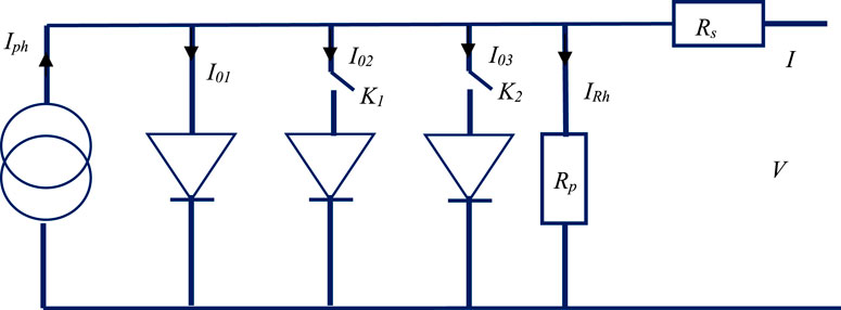
Figure 1. Solar cell model’s equivalent circuit.

Figure 1 presents the different parameters of solar cells, such as five, seven, and nine parameters. This parameter determines the properties of an implicit nonlinear equation that governs the I–V and P–V relationship in the PN junction.

The model with a single diode offers a more explicit mathematical depiction of a solar cell’s electrical characteristics. It assumes that the solar cell may be effectively represented as a single diode connected to an electrical source. Although simplistic, the single-diode model covers the most important characteristics of the solar cell’s electrical reaction while being computationally feasible. In the SDM, the I–V relationship of a PV cell can be described as follows:

Equation 1 presents the implicit equation characterizing the behavior of the terminal of the solar cell and PVM source, and it can be presented as follows:

$I=I_{ph}-I_{01}\left(e^{\frac{V+I{R}_s}{n_1{V}_t}}-1\right)-{K_{1}I}_{02}\left(e^{\frac{V+I{R}_s}{n_2{V}_t}}-1\right)-{K_{2}I}_{03}\left(e^{\frac{V+I{R}_s}{n_3{V}_t}}-1\right)-\frac{V+I{R}_s}{R_P}.(1)$

The factors K₁ and K₂ determine the number of diodes; if K₁ ≠ 0, there are two diodes, and when K₁ ≠ 0 and K₂ ≠ 0, then there are three diodes.

This equation is combined from the photocurrent ($I_{ph}$) in parallel with the diodes, parallel resistances, and series resistance, and each diode has the currents of reverse saturation ($I_{01},I_{02},I_{03}$) for each diode, and diode ideality factor. The single-, double-, and triple-diode equations can be given as follows:

$\left\{\begin{array}{l}I=I_{ph}-I_{01}\left(e^{\frac{V+I{R}_s}{n_1{V}_t}}-1\right)-\frac{V+I{R}_s}{R_P}\\ I=I_{ph}-I_{01}\left(e^{\frac{V+I{R}_s}{n_1{V}_t}}-1\right)-I_{02}\left(e^{\frac{V+I{R}_s}{n_2{V}_t}}-1\right)-\frac{V+I{R}_s}{R_P}\\ I=I_{ph}-I_{01}\left(e^{\frac{V+I{R}_s}{n_1{V}_t}}-1\right)-I_{02}\left(e^{\frac{V+I{R}_s}{n_2{V}_t}}-1\right)-I_{03}\left(e^{\frac{V+I{R}_s}{n_3{V}_t}}-1\right)-\frac{V+I{R}_s}{R_p}\end{array}\right..(2)$

The three-diode model can better represent the actual behavior of solar cells. It makes it possible to consider more precisely the losses and non-idealities that can affect the performance of a solar cell.

The PV module consists of many cells that are linked in parallel for greater current and linked in series for enhanced voltage. The numerical formula for a single diode in a photovoltaic module is defined as follows:

$I=N_p{I}_{ph}-N_p{I}_{01}\left(e^{\frac{N_{p}V+N_{s}I{R}_s}{N_p{N}_s{n}_1{V}_t}}-1\right)-\frac{N_{p}V+N_{s}I{R}_s}{N_p{N}_s{R}_p},(3)$

where Ns and Np are the total quantity of solar cells linked in series and in parallel, respectively.

Equation 4 may be represented simply as follows:

$I=I_{phm}-I_{0m1}\left(e^{\frac{V+I{R}_{sm}}{n_{m1}{V}_t}}-1\right)-\frac{V+I{R}_{sm}}{R_{pm}}.(4)$

The same is found for double and triple diodes:

$\left\{\begin{array}{l}I=I_{phm}-I_{0m1}\left(e^{\frac{V+I{R}_{sm}}{n_{m1}{V}_t}}-1\right)-I_{0m2}\left(e^{\frac{V+I{R}_{sm}}{n_{m2}{V}_t}}-1\right)-\frac{V+I{R}_{sm}}{R_{pm}}\\ I=I_{phm}-I_{0m1}\left(e^{\frac{V+I{R}_{sm}}{n_{m1}{V}_t}}-1\right)-I_{0m2}\left(e^{\frac{V+I{R}_{sm}}{n_{m2}{V}_t}}-1\right)-I_{0m3}\left(e^{\frac{V+I{R}_{sm}}{n_{m3}{V}_t}}-1\right)-\frac{V+I{R}_{sm}}{R_{pm}}\end{array}\right.,(5)$

where $I_{phm}=N_p{I}_{ph}$, $I_{0m1}={N_{p}I}_{01}$, $I_{0m2}={N_{p}I}_{02}$, $I_{0m3}={N_{p}I}_{03}$ ${n_{m1}=N_{s}n}_1$, ${n_{m2}=N_{s}n}_2$, ${n_{m3}=N_{s}n}_3$, $R_{sm}=\raisebox{1ex}{$N_s$}\!\left/ \!\raisebox{-1ex}{$N_p$}\right.R_s$, and $R_{pm}=N_s{R}_p$.

The equations provided for each model show how the I–V interaction of a solar cell and a PVM changes with factors such as radiation from the sun, environmental temperature, speed of the wind, and dust, and it depends on standard deviations found in data sheets.

4 Objective function

The implemented objective function should extract, determine, and evaluate the unidentified parameters from the measured data of the current and voltage of the four solar cells and PVM given in the previous section. In literature research, a three-objective function was used to identify the known parameters of solar cells and PVMs, such as the RMSE (Frías-Paredes et al. (2018), Easwarakhanthan et al. (1986)), sum of squared error (SSE) (Tong and Pora, 2016), and the IAE (Taleshian et al., 2023). The cost function is constructed based on $I=f\left(V\right)$ using the unknown parameters of the solar cell and PVM as the parameters’ constraints. During the tuning procedure, all constraint parameters are described by a vector for single, double, and triple diodes.

The unknown parameters of the solar cells with single, double, and triple diodes are the constraints’ function and are defined as $x_1=\left[I_{ph}{I}_{01}{n}_1{R}_s{R}_p\right]$, $x_2=\left[I_{ph}{I}_{01}{I}_{02}{n}_1{n}_2{R}_s{R}_p\right]$, and $x_3=\left[I_{ph}{I}_{01}{I}_{02}{I}_{03}{n}_1{n}_2{n}_3{R}_s{R}_p\right]$, respectively.

For single, double, and triple diodes in the PVM or generator, the constraints’ function can be defined as $x_{1m}=\left[I_{phm}{I}_{0m}{n}_m{R}_{sm}{R}_{pm}\right]$, $x_{2m}=\left[I_{phm}{I}_{0m1}{I}_{0m2}{n}_{m1}{n}_{m2}{R}_{sm}{R}_{pm}\right]$, and $x_{3m}=\left[I_{phm}{I}_{0m1}{I}_{0m2}{I}_{0m3}{n}_{m1}{n}_{m2}{n}_{m3}{R}_{sm}{R}_{pm}\right]$, respectively.

The objective function is used to optimize solar cells and PVMs on large amounts of space and extract their parameters. Equation 5 shows how the cost function base in the unknown parameters is generated using the $I=f\left(V\right)$ characteristic curves of the solar cell and PVM for single, double, and triple diodes.

$\left\{\begin{array}{l}{f}_{1,2,3}\left(V,I\right)=I-I_{ph}+{\displaystyle \sum _{i=1}^3}{I}_{0i}\left(e^{\frac{V+I{R}_s}{n_i{V}_t}}-1\right)+\frac{V+I{R}_s}{R_P}\\ f_{1m,2m,3m}\left(V,I\right)=I-I_{phm}+{\displaystyle \sum _{i=1}^3}{I}_{0mi}\left(e^{\frac{V+I{R}_{sm}}{n_{mi}{V}_t}}-1\right)+\frac{V+I{R}_{sm}}{R_{pm}}\end{array}\right.,(6)$

where $f_1,f_2,f_3$ and $f_{1m}$, $f_{2m}$, and $f_{3m}$ present the cost functions for the one, two, and three diodes for the solar cell and PVM, respectively, for the three case studies.

In order to determine the fundamental unknown parameters $I_{ph},I_{01,}{I}_{02,}{I}_{03,}{n}_1,n_2,n_3,R_s,\text{and\hspace{0.17em}}{R}_p$, we optimized the model of Equation 6 by minimizing the Integral of Absolute Error (IAE) function across the experimental and theoretical curves. The used experimental data are widely used in the research literature by various papers. In this research, we utilize $f\left(x\right)=IAE\left(I,V\right)$ as the cost function to maximize $I=f\left(V\right)$ of each model by minimizing this function. The nine objective functions are optimized under the following conditions presented in Supplementary Table S1 in the Supplementary Material section.

5 Earthworm optimization algorithm in foraging

The EOA was implemented to identify the unknown parameter of different technologies of solar cells and PVMs for one, two, and three diodes. The process of using the EOA in the solar cell and PVM can be detailed as presented in the following:

We start by initializing the EOA. In this step, we define the number of earthworms which possess a determined number of parameters depending on the properties of the PVM or solar cell by using the Roulette wheel function, as follows:

$P=\left\{\begin{array}{l}\left[I_{ph}{I}_{01}{n}_1{R}_s{R}_p\right]forsolarcellsinglediode\\ \left[I_{ph}{I}_{01}{I}_{02}{n}_1{n}_2{R}_s{R}_p\right]forsolarcelldoublediodes\\ \left[I_{ph}{I}_{01}{I}_{02}{I}_{03}{n}_1{n}_2{n}_3{R}_s{R}_p\right]forsolarcelltriplediodes\end{array}\right..(7)$

After initializing and defining the unknown parameters, we determine an appropriate number of iterations and randomly initialize the earthworm parameters, ensuring that optimization occurs within each parameter’s restrictions. Furthermore, in the optimization loop, we continue to cycle through the following stages until a halting condition is reached, which is commonly specified as achieving the maximum number of iterations. This step can be given in two steps, as follows:

• Evaluating each earthworm using the solar cell parameters to obtain the predicted currents.

• Calculating the error for each earthworm using the error function (Equation 6) focusing on a minimum error.

$IAE=\left|f\left(V,I\right)\right|.(8)$

We update each earthworm’s parameters using specialized updated equations that include information from other earthworm parameters in the algorithm:

${P_{ji}}^{t+1}={P_i}^t+r\left(P_{i_{best}}-{P_i}^t\right),(9)$

where i is the number of parameters, t is the number of iterations, j is the number of earthworms, $P_{i_{best}}$ is the best earthworm (best parameters), and r is the random defined as $\mathrm{r}\in \left[0,0.02\right]$ for current lower than 1 A and $r\in \left[0,0.1\right]$ for current higher than 1 A.

After completing the required number of repetitions, we extract the parameters associated with the best-performing earthworm. These parameters are the fitted values of the solar cell model that best match the experimental data.

This EOA is simple and effective, allowing for a complete investigation of the search space. It is particularly useful for determining the best solution from a large number of options. Figure 2 shows the flowchart used for the EOA based on Equations 8, 9.

Figure 2

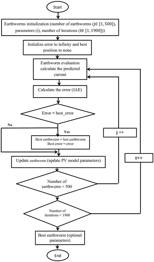
Figure 2. EOA flowchart.

6 Statistical criteria assessment

Estimation error occurs when there is a persistent difference between the measured and approximated results. Within any of the predictive approaches, it is critical to examine and measure the prediction error and precision (Oliva et al., 2017). In general, estimates are susceptible to being both too high and too low, as is typical with independent estimates. A successful prediction approach has zero prediction metrics, which means that it has a total estimation error of 0. If the anticipated discrimination is zero, the positive and negative fitting faults even out. It is generally recognized that a method with very little precision (strong comparative error) has negligible fit discrimination, whereas a system with high accuracy (with a low comparative error) has considerable forecast bias. The qualities of the results will be evaluated following different statistical criteria, as described in Supplementary Table S2 presented in the Supplementary Material.

7 Experimental results

To extract the parameters of the photodiode model, this technique simulates the optimization behavior of a swarm of earthworms during foraging. An initial population of “earthworms” is generated, with each earthworm representing a randomly initialized set of parameters within predefined constraints. In each iteration, the algorithm evaluates the error between the measured current and the model-predicted current for every earthworm using Equation 8. If an earthworm’s error is lower than the best-known error, it replaces the current optimal solution.

Each earthworm then updates its position (parameters) by moving toward the best-performing earthworm, with the exploration intensity regulated by Equation 4. The updated parameters are constrained to remain within permissible bounds.

This process repeats for a fixed number of iterations, and the algorithm ultimately returns the best parameter set that is found.

The efficiency of the optimization algorithm depends primarily on the proper tuning of its key parameters. The optimal configurations were determined as follows:

• Standard model: population size = 800 earthworms, iterations = 19,000, and natural noise variance = 0.07.

• Binary dyad: population size = 500 earthworms, iterations = 19,000, and natural noise variance = 0.3.

• Ternary dyad: population size = 800 earthworms, iterations = 19,000, and natural noise variance = 0.03.

We evaluated parameter impacts by testing multiple values while keeping other factors constant. Results demonstrate that insufficient population sizes or iteration counts significantly reduce the quality of the solution. Our experiments show that population sizes of 500–800 earthworms combined with approximately 19,000 iterations achieve an optimal balance between accuracy and computational efficiency for both binary and ternary dyads.

• For the RTC France implementation, the parameter optimization times were as follows:

• One-diode model: 15 min 30 s.

• Two-diode model: 13 min 15 s.

• Three-diode model: 19 min 39 s.

This part deals with the implementation of the EOA to reconstruct and approximate the I–V and P–V characteristic curves of the SD, DD, and TD models of solar cells and PVMs in three different case studies. The first test scenario deals with the commercial solar cell fabricated by RTC France, with a diameter of 57 mm. The experimental I–V data were measured at T = 33°C under full solar irradiation. The second test scenario is the PVMs, commercialized under the name PhotoWatt PWP-201, which is composed of 36 cells connected in series. The experimental I–V characteristics were determined at T = 45 °C and G = 1,000 W/m² (Hosseini Rad and Abdolrazzagh-Nezhad, 2020). The third test scenario is utilized to assess the Schutten Solar STM-40/36 monocrystalline solar module. This assessment is based on experimental data obtained at T = 51 °C and G = 1,000 W/m². The module, measuring 38 mm by 128 mm, consists of 36 cells connected in series (Ns = 36, Np = 1) (Zhang et al., 2011). All these units are frequently employed in scientific literature to evaluate parameter estimation methods for similar models, and the I–V experimental data are sourced from the study by Cotfas et al. (2016). The suggested method’s efficiency is evaluated and confirmed using experimental data from many solar modules produced using various production processes. The resulting findings are compared to several empirical and meta-heuristic techniques, such as the gray wolf optimizer (GWO) (Mirjalili et al., 2014), the genetic algorithm with convex combination crossover (GA-CCC) (Hamid et al., 2019; Jervase et al., 2001; Zagrouba et al., 2010), whale optimization algorithm (WOA) (Oliva et al., 2017), particle swarm optimization (PSO) (Taleshian et al., 2023; Oliva et al., 2017; Ye et al., 2009; Ebrahimi et al., 2019), sine–cosine algorithm (SCA) (Mirjalili, 2016), and multiverse optimizer (MVO) (Batzelis et al., 2016). The Improved Chaotic Whale Optimization Algorithm (Oliva et al., 2017), the Lambert W-function (LW) (Zhang et al., 2011), Genetic Algorithms (GA) (Jervase et al., 2001). Numerical methods usually use nonlinear optimization techniques, such as the Newton–Raphson method (NRM) (Easwarakhanthan et al., 1986), conductivity method (CM) (Chegaar et al., 2001), harmony search (HS) (Askarzadeh and Rezazadeh, 2012), moth–flame optimization (MFO) (Mirjalili, 2015), pattern search (PS) (Mirjalili, 2015), BAT (Gandomi et al., 2013), slime mould algorithm (SMA) (Li et al., 2020), hunger games search (HGS) (Lim et al., 2024), hybridized interior search algorithm (HISA) (Kle et al., 2019), cuckoo search (CS) algorithm (Chen and Yu, 2019), simulated annealing algorithm (SA) (El-Naggar et al., 2012), modified gray wolf optimizer (mGWO) (Mittal et al., 2016), enhanced gray wolf optimization algorithm (EGWO) (Joshi and Arora, 2017), improved GWO (IGWO) (Long et al., 2017), alpha-guided GWO (AgGWO) (Hu et al., 2019), PSO-WOA (Xiong et al., 2018), artificial bee colony (ABC) algorithm (Oliva et al., 2014), real-coded BBO with Gaussian mutation (RCBBOG) (Gong et al., 2010), blended BBO (BlendedBBO) (Ma and Simon, 2011), and Monte Carlo optimization and parallel resistance adjustment (Wardi et al., 2025).

7.1 Test scenario 1: French RTC solar cell

The implemented technique is used in the first test scenario to identify the electrical parameters of SD, DD, and TD models of mono-crystalline silicon solar cells commercialized under French RTC, with 57-mm diameter of each cell. The parameters recovered by several techniques (I_ph, I₀₁, I₀₂, I₀₃ n₁, n₂, n₃, R_s, and R_p) for the single-, double-, and triple-diode models are compared in Table 1, and their performance is assessed using error metrics such as RMSE and MAE.

Table 1

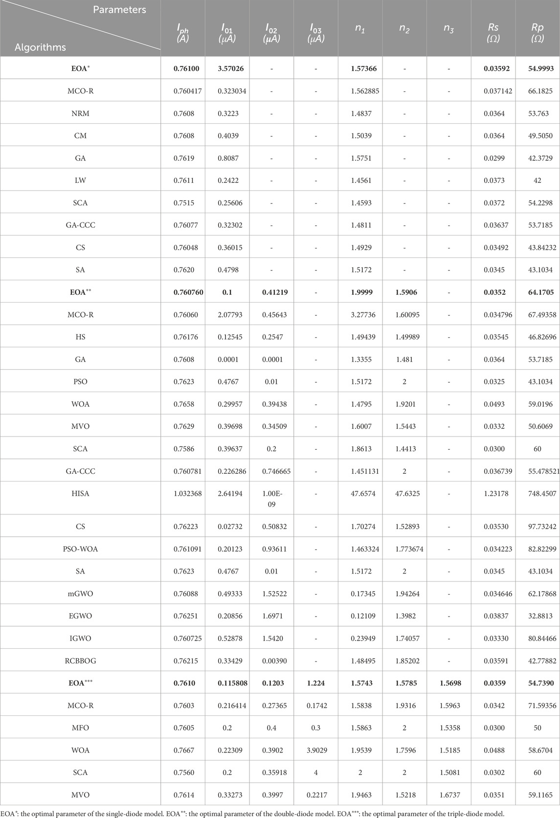
Table 1. Comparative analysis of the RTC France solar cell SD model.

To understand the qualities of the characteristic curves evaluated by the implemented EOA method, the statistical criteria are calculated and evaluated. Figures 3, 4 illustrate the compared RMSE and MAE of the used algorithm with other techniques and methods published in the research field for the three models (SD, DD, and TD). The algorithm that produces the best results, with the lowest RMSE and MAE, is the EOA. The EOA’s consistency and dependability are confirmed by a statistical examination of its performance. RMSE is a popular statistic for assessing the precision of prediction models, with lower values indicating greater performance. In this investigation, the approaches are ordered by their RMSE values, which vary from 0.002 to 0.018 for single, double and triple diode model. The approach with the lowest RMSE (approximately 0.002) for the three types of cells (SD, DD, and TD) has an excellent precision and is deemed the top performer. This approach is expected to have the least differences between anticipated and experimental results, showing a high predictive performance. The technique with the largest RMSE (approximately 0.018) performs inadequately, indicating important inaccuracies in its estimations. To enhance precision, this procedure may need to be refined deeper or used with an alternative approach. The variance of RMSE values among approaches demonstrates the variety in their performance. Methods with RMSE values in the lower range (e.g., 0.002–0.008) for SD, DD, and TD are more trustworthy, but those with higher RMSE values (e.g., 0.012–0.018) may require improvement.

Figure 3

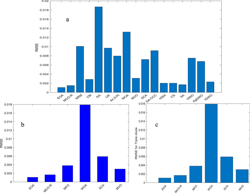
Figure 3. Compared RMSE and MAE for different methods: (a) single diode, (b) double diode, and (c) triple diode.

Figure 4

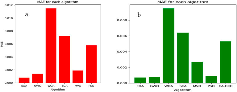
Figure 4. Compared MAE for different methods and techniques: (a) single diode and (b) double diode.

This analysis is critical for determining the most efficient approach for a certain application and understanding the trade-offs between accuracy and processing complexity, among other things. In conclusion, the figure clearly represents the RMSE values for several approaches, allowing for the identification of the best-performing method with the lowest error and the method with the largest error, which may require improvement. This study is critical for determining the best strategy for modeling predicted activities. Figure 4 presents the compared MAE for single- (a) and double-diode (b) models. The algorithm that produces the best results, with the lowest RMSE and MAE, is the EOA for both cell types.

Figure 5 illustrates the calculated errors metric for single diode in terms of the standard deviation (SD) (a), time series (TS) (c), normalized frequency modulation (NFM) (b), and auto-correlation function (ACF) (c). Figure 5a shows that the SD values are approximately 3 × 10⁻³ for the used method. TS and NFM are represented in Figures 5b,c, for single diode with respect to the quality of the estimated measurements. The values range from −1 to +1, and for NFM, identification is challenging. TS outperforms the NFM in identifying the estimation precision.

Figure 5

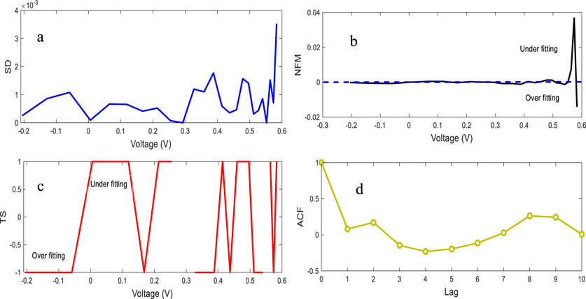
Figure 5. Statistical metric analysis of SD model, covering (a) SD, (b) NFM, (c) TS, and (d) ACF obtained by EOA.

Figure 6 presents the IAE and RE of the single-diode model for the French RTC solar cell. The IAE and RE are compared with different methods, such as PS (Mirjalili (2015), Easwarakhanthan et al. (1986), Shaheen et al. (2023), Bouzidi et al. (2007), Louzazni et al. (2020)), GA, and GA-CCC. The IAE and RE of the used algorithm present lower values than other techniques and methods. The EOA exhibits a high quality compared to the analytical, iterative methods and algorithms.

Figure 6

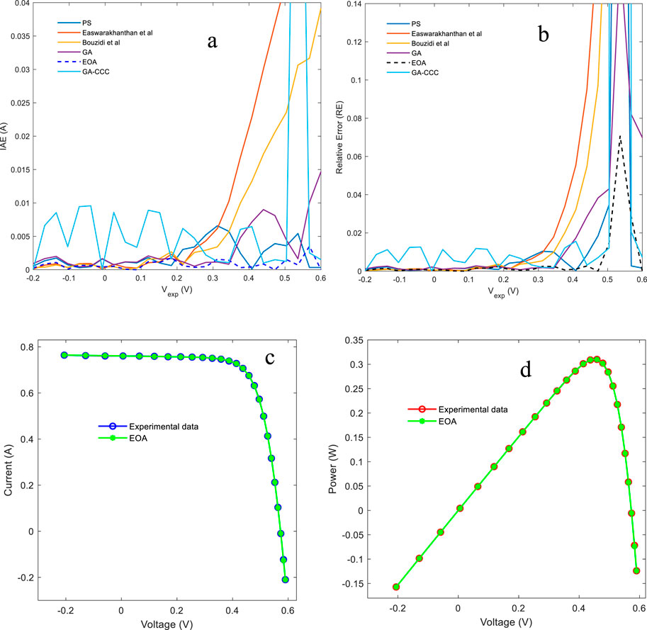
Figure 6. (a) IAE, (b) RE, (c) I–V, and (d) P–V curves for SD.

Figures 6b,c, present the comparison of the reconstructed I–V and P–V characteristic curves using the extracted parameters of the RTC France Silicon solar cell. The theoretical curves of I–V and P–V are very close to the experimental data.

For the double-diode model, the statistical error metrics compared to other techniques are presented in Figure 8. This figure illustrates the SD, TS, NFM, and ACF. The maximum value of the SD is approximately 0.01 and that of NFM is approximately 0.08, in which a few values were over fitting when the values were near 0.6 V. Figure 7d demonstrates the autocorrelation test function of the calculated values using the EOA methods. The RTC France Silicon solar cell training evaluation yields results between −1 and 1.

Figure 7

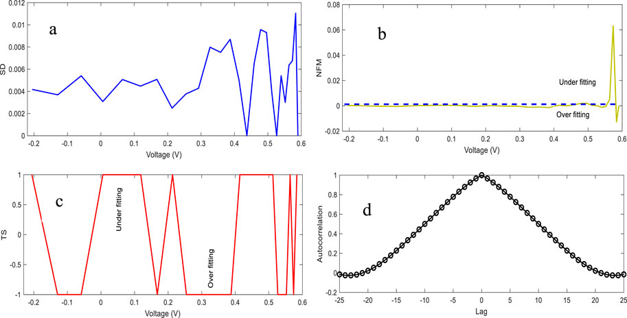
Figure 7. Statistical analysis of DD, covering (a) SD, (b) NFM, and (c) TS obtained by EOA, and (d) Autocorrelation.

Figure 8 provides more thorough comparisons of the reconstructed double-diode models of the RTC France Silicon solar cell to show that the proposed method could be utilized for solar cell approximation in terms of IAE and RE. The comparison between the EOA and GA-CCC (Taleshian et al., 2023), PS (Dkhichi et al., 2014), SA (Hamid et al., 2019), and HS (Sajawal Ur Rehman Khan et al., 2018) shows that the implemented method is better in terms of low values in IAE and RE.

Figure 8

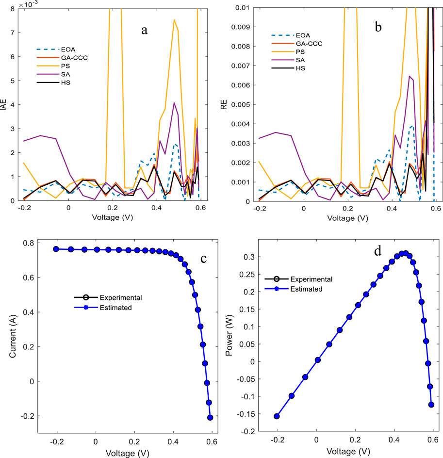
Figure 8. Comparison of (a) IAE, (b) RE, and the reconstructed (c) I–V and (d) P–V characteristics of DD model.

The reconstructed I–V and P–V characteristic curves of double diodes are presented in Figure 8c and d using the extracted parameters of the RTC France Silicon solar cell. The theoretical curves of I–V and P–V are very close to the experimental data for the single, double, and triple diodes, respectively.

For the triple-diode model, Table 1 compares the parameters (I_ph, I₀₁, I_02, I₀₃, n₁, n₂, n₃, R_s, and R_p) and assesses the error metrics (RMSE, RE, and IAE) across methods (Bo et al., 2022). Once more, the EOA yields the most precise results with the fewest mistakes. To verify the algorithm’s robustness, Figure 9 provides a statistical analysis that includes TS, NFM, SD, and ACF.

Figure 9

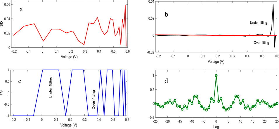
Figure 9. Statistical analysis of the triple-diode model, covering (a) SD, (b) NFM, (c) TS, and (d) ACF obtained by EOA.

Figure 10 illustrates the minimal error rates of the EOA by highlighting the IAE and RE across voltage levels for the triple-diode model. Finally, to verify the algorithm’s robustness, Figures 10c and d show a great match and support the accuracy of the method by comparing the experimental I–V and P–V curves with those modified using the EOA.

Figure 10

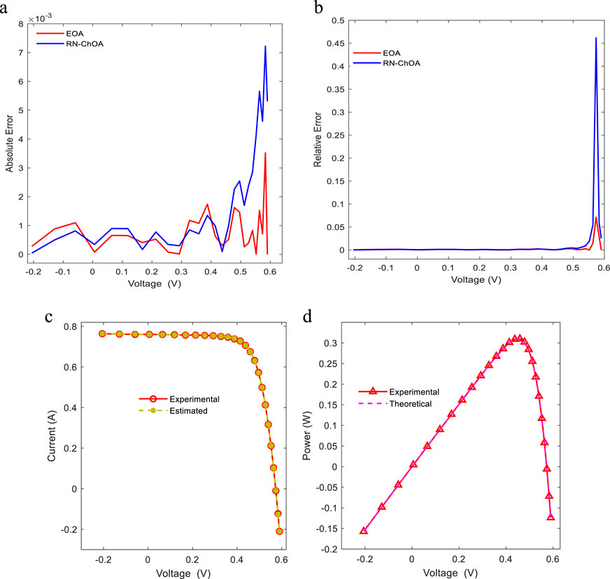
Figure 10. (a) IAE, (b) RE, and the reconstructed characteristics (c) I–V and (d) P–V using EOA compared with experimental data for TD.

For more validation of triple-diode model parameters’ extraction, Figures 10c and d illustrate the IAE and RE of the EOA compared with RN-ChOA (Hosseini Rad and Abdolrazzagh-Nezhad, 2020). Once more, the EOA yields the most precise results with the fewest mistakes. Figure 10 illustrates the minimal error rates of the EOA by highlighting the IAE and RE across voltage levels for the TD model.

7.2 Test scenario 2: PVM Photowatt-PWP 201

In the second test scenario, the EOA is used to identify the unknown parameters of the photovoltaic module known as Photowatt-PWP 201 (pour le module Photowatt-PWP 201), which is made up of 36 series-connected polycrystalline silicon cells, and to extract the electrical parameters of single-, double-, and triple-diode models. The parameters (I_ph, I₀₁, I₀₂ I₀₃ n₁, n₂, n₃, R_s, and R_p) extracted by the EOA and other techniques and methods for the single-, double-, and triple-diode models are compared in Table 2.

Table 2

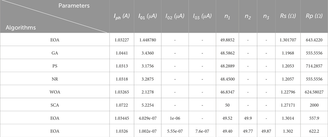
Table 2. Comparative analysis of the Photovoltaic module Photowatt-PWP 201.

Figure 11 presents the compared RMSE for the single diode compared with HGS, SMA, BAT, GA, PS, NR, WOA, and SCA, and the second illustrates the REMS for the TD and DD models. The third compares the MAE for the three models, which present the MAE for the double-diode model presenting the low values. The compared MAE in Figure 14 shows a clear EOA supplementary to the MAE of the three models (SD, DD, and TD).

Figure 11

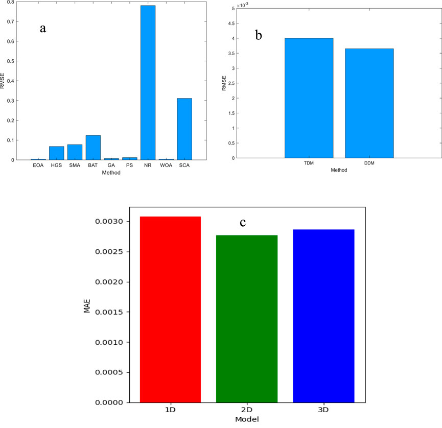
Figure 11. (a) RMSE of SDM, (b) compared RMSE of DDM and TDM, and (c) compared MAE of SDM, DDM, and TDM.

The statistical errors for the single-diode model are illustrated in Figure 12. Figure 12 clearly shows that the results of the statistical criteria calculated for the single-diode model using SD, NFM, TS, and ACF exhibit low errors when using the EOA.

Figure 12

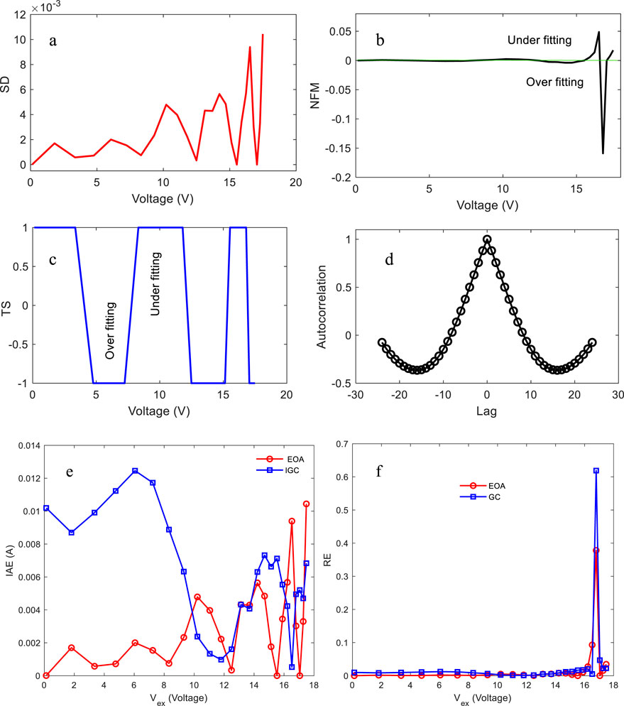
Figure 12. Statistical analysis, covering (a) standard deviation (SD), (b) normalized frequency modulation (NFM), (c) time series (TS), (d) autocorrelation function (ACF), (e) IAE, and (f) RE of the single-diode model obtained by EOA for Photowatt-PWP 201.

Figures 12e,f, illustrate the IAE and RE of the single-diode model calculated using the generated data points using the EOA of the photovoltaic module Photowatt-PWP 201 compared with GC. The proposed and used EOA method presents low values in IAE and RE when compared to the GC algorithm.

The second part is about the double-diode PVM Photowatt-PWP 201. The calculated statistical errors based on the pair data generated by the EOA for SD, NFM, TS, and the ACF are presented in Figure 13. The statistical errors are calculated to verify the algorithm’s robustness, and Figure 13 provides a statistical analysis that includes TS, NFM, SD, ACF, IAE, and RE. Figure 13 illustrates a great match and supports the accuracy of the method by comparing the experimental I–V and P–V curves with those modified using the EOA.

Figure 13

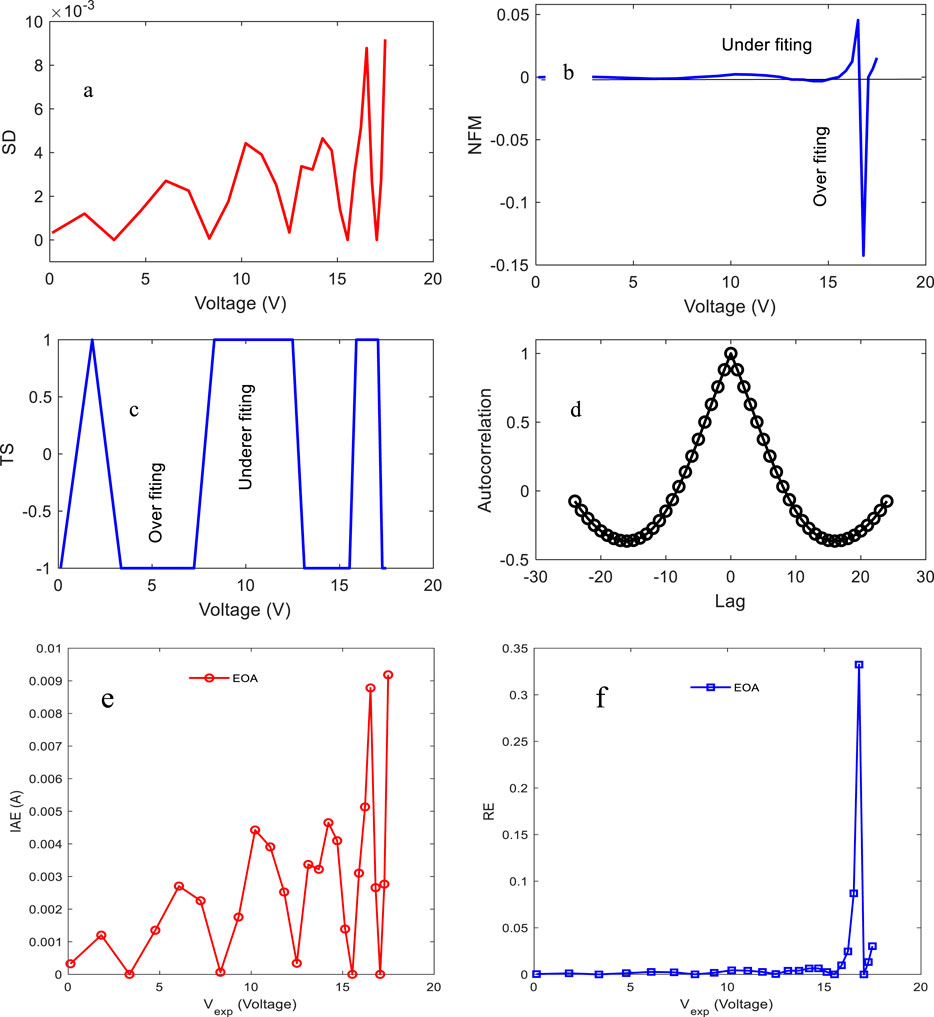
Figure 13. Statistical analysis of the double-diode model, covering (a) standard deviation (SD), (b) normalized frequency modulation (NFM), (c) time series (TS), (d) autocorrelation function, (e) IAE, and (f) RE for the double-diode model of Photovoltaic module Photowatt-PWP 201.

To validate the calculated data point of the double-diode model for the PVM Photowatt-PWP 201, we calculate the IAE and RE and present them in Figures 13e, f. These data show a low value in IAE and RE, which validates that the EOA can be used in the parameter’s extraction in the double-diode model.

The statistical analysis of the triple-diode model is presented in Figure 14 using data points of the PVM Photowatt-PWP 201 approximated using the EOA. Figure 14 illustrates SD, NFM, TS, and the ACF.

Figure 14

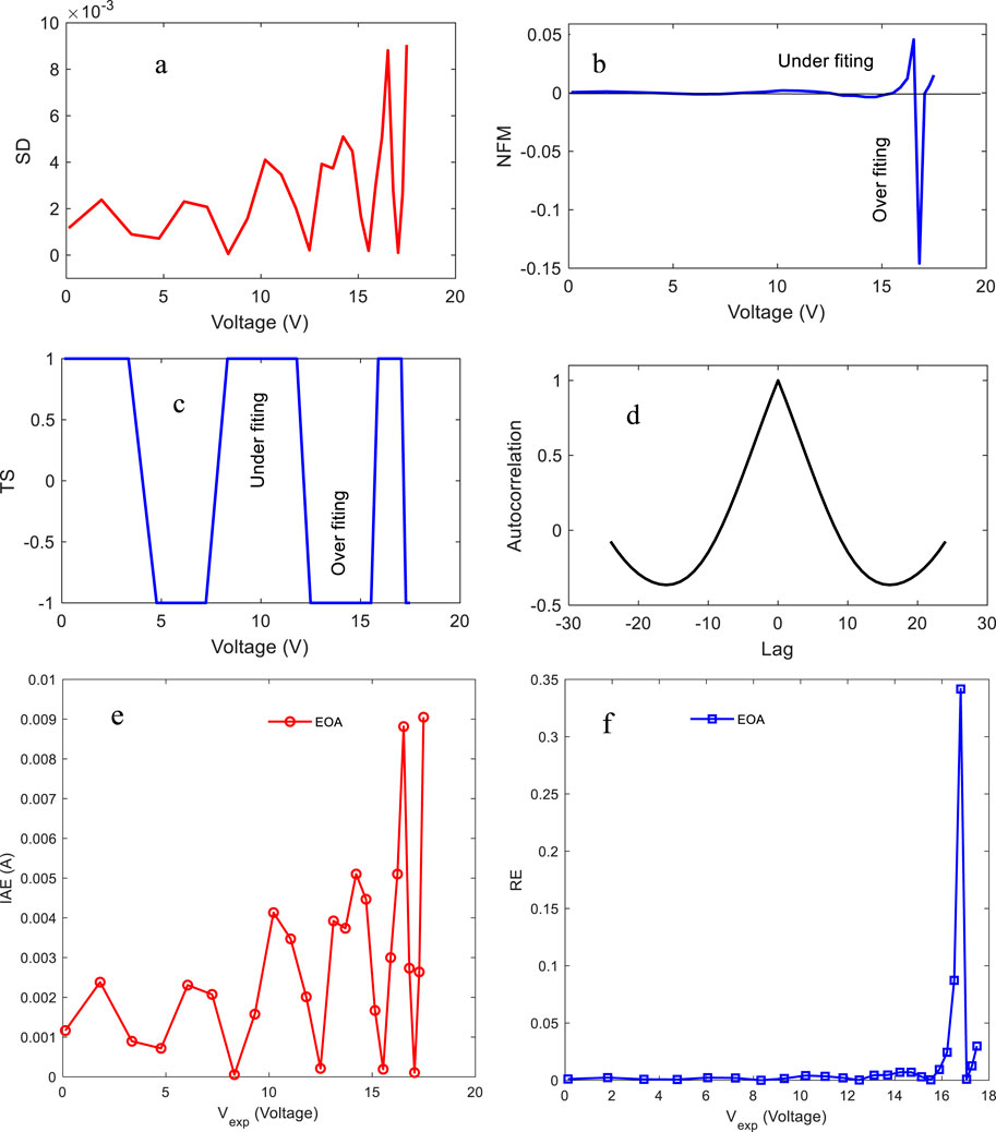
Figure 14. Statistical analysis of the triple-diode model, covering (a) standard deviation (SD), (b) normalized frequency modulation (NFM), (c) time series (TS), (d) autocorrelation function, (e) IAE, and (f) RE for the triple-diode model of Photovoltaic module Photowatt-PWP 201.

The reconstruction of the I–V and P–V characteristic curves for each model (SD, DD, and TD) is presented in Figure 15. The reconstructed characteristic curves using the proposed algorithms show a high agreement with the experimental data points for single, double, and triple diodes of the PVM Photowatt-PWP 201 cell.

Figure 15

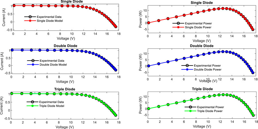
Figure 15. Compared reconstructed characteristic I–V and P–V curves with experimental data for single, double, and triple diodes of Photovoltaic module Photowatt-PWP 201 cell.

7.3 Test scenario 3: Schutten Solar STM6-40/36 monocrystalline

In the third application, the EOA is used to assess the Schutten Solar STM-40/36 monocrystalline PVM. The EOA is used based on the experimental data of the current and voltage to extract and approximate the unknown parameter of the proposed PVM. Table 3 compares the extracted parameters using the EOA-based experimental data. The EOA outperformed other algorithms that were examined. Other algorithms, on the other hand, such as BAT and SMA, showed less consistent outcomes and larger RMSE values.

Table 3

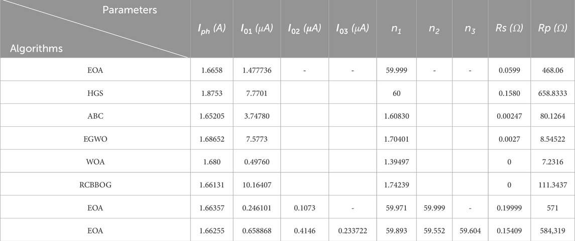
Table 3. Comparative analysis of the Schutten Solar STM6-40/36 monocrystalline for single-, double-, and triple-diode models.

Figure 16 depicts the TS, NFM, and ACF. Figure 16 illustrates the calculations and NFM in terms of the estimated measurement quality for the calculated and estimated current using the extracted parameters using the EOA. The values range from −1 to +1, and NFM’s identification is tough. In determining estimating precision, the TS outperforms the NFM.

Figure 16

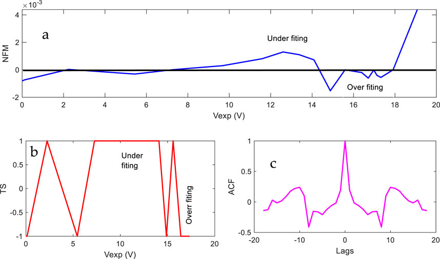
Figure 16. Statistical analysis of the SD: (a) TS, (b) NFM, and (c) ACF obtained by EOA.

Figure 17 presents the compared calculated current based on the unknown parameters obtained using the EOA. On comparison, the measured current and estimated current using the EOA appear to be the same. The illustrated curve is linear, which means that the approximated data are very near to those measured.

Figure 17

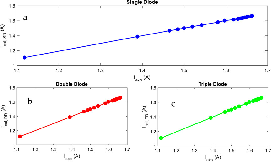
Figure 17. Theoretical power vs. experimental power for (a) SD, (b) DD, and (c) TD models.

Figure 18 shows the absolute error of current (IAE) and relative error (RE) for three distinct photovoltaic cell models: single-diode, double-diode, and triple-diode models. The first row (Figures 18a, b) shows the single-diode model, in which both IAE and RE are low at lower voltages but considerably increase beyond 15V, suggesting poorer accuracy at higher voltages. The second row (Figures 17c, d) represents the double-diode model, which has more accuracy than the single-diode model, with modest error fluctuations and localized peaks at 15 V and 18 V. Finally, the third row (Figures 18e,f) illustrates the triple-diode model, which decreases the overall error but increases oscillations, notably in the mid-voltage band. The overall trend indicates that increasing model complexity improves accuracy; however, the triple-diode model shows larger fluctuations in RE and IAE, which might be attributable to parameter sensitivity.

Figure 18

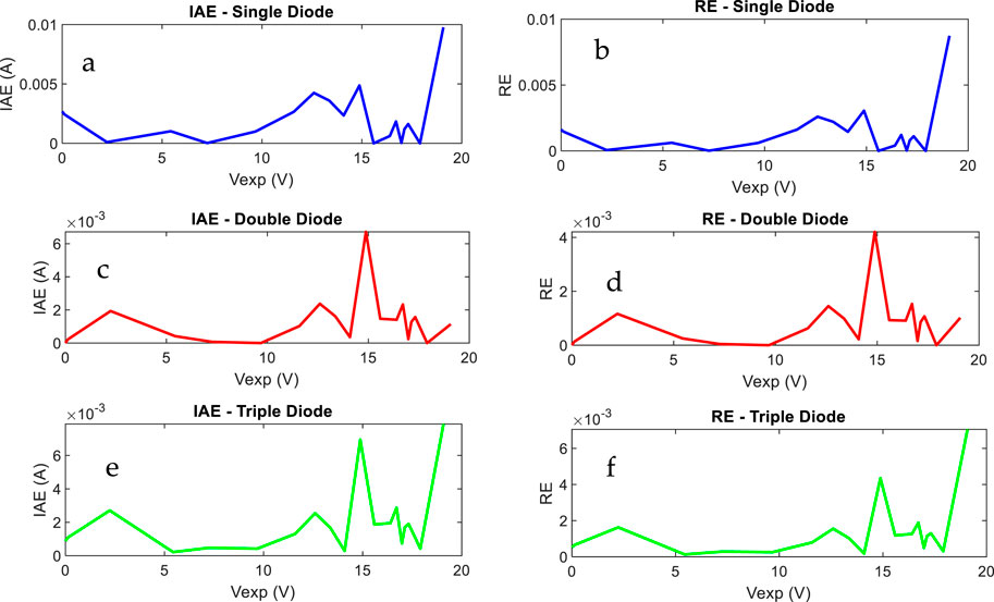
Figure 18. IAE for (a) single diode, (b) double diode, (c) triple diode and RE for (d) single diode, (e) double diode and (f) triple diode.

Figure 19 illustrates the reconstructed I–V and P–V curves obtained using the unknown parameter extracted by the EOA compared to the measured data. This comparison shows a good agreement among the approximated data and measured data for single, double, and triple diodes.

Figure 19

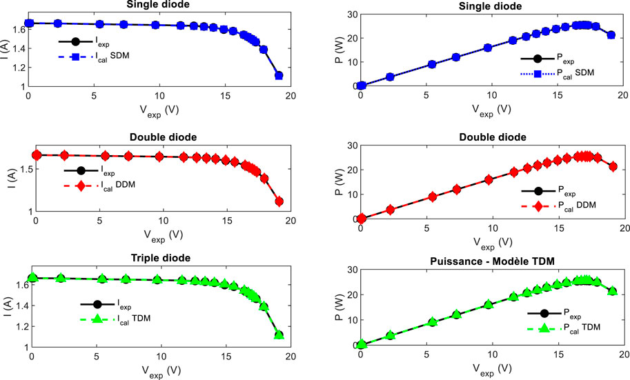
Figure 19. Comparison among measured and approximated I–V and P–V curves for single, double, and triple diodes.

The efficiency of the EOA in precisely simulating solar cell performance for single-, double-, and triple-diode configurations of the Schutten Solar STM6-40/36 module is demonstrated by this thorough analysis across tables and figures presented in Figure 20. Both models presented in the NFM plot have modest error at lower voltages, but deviations rise beyond 15 V, with the 3D model exhibiting more variations, suggesting potential overfitting at high voltages. The TS results for double-diode models underfit at low voltages and those for the triple-diode model overfit at higher voltages, demonstrating the trade-off between model complexity and generalization. The ACF over different lags for double- and triple-diode models captures similar data patterns, but the TD model has slightly higher peaks, indicating a stronger correlation with experimental data. Overall, the TD model offers a better fit at mid-range voltages but risks overfitting, whereas the DD model underfits at lower voltages but remains stable.

Figure 20

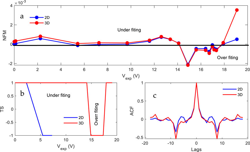
Figure 20. Statistical analysis of the double-diode and triple-diode models, covering (a) NFM, (b) TS, and (c) ACF obtained by EOA.

8 Discussions

It is important to note that very small mistakes, such as RE values close to zero and decreased IAEs, imply a high degree of agreement between algorithm predictions and actual experimental data. Higher errors, on the other hand, indicate a significant difference between expectations and experimental results. The results provided by the EOA and GA-CCC algorithms may be analyzed more thoroughly to assess their respective performances. From the perspective of the EOA method, the RE and IAE appear to be low overall, indicating a close match between predictions and actual experimental values. This suggests that the EOA has a reasonable ability to model experimental data. The findings reported for various techniques, assessed in terms of RMSE and MAE, vary significantly. The EOA method has the lowest RMSE of any algorithm, demonstrating extremely low error dispersion between predictions and actual values. Again, the EOA method has the smallest MAE, suggesting minimal average absolute errors between predictions and actual observations. These data show that the EOA seems to perform the best in terms of accuracy.

9 Conclusion

In this paper, we deal with the identification through optimization of a cost function based on the parameters of the solar cell and PVM. By using the measured data points of I–V pairs and the constraints for each parameter in single, double, and triple diodes, the EOA technique is implemented to extract each parameter. Three different case studies were implemented using one solar cell, namely, the French RTC solar cell, and two different PVMs: Photowatt-PWP 201 and Schutten Solar STM6-40/36 monocrystalline solar modules. In order to validate the reconstructed I–V and P–V curves, various statistical criteria are calculated, such as IAE, RE, SD, RMSE, MAE, TS, and NFM. The comparison is made for single, double, and triple diodes in each case study. The obtained results have been compared with several recent algorithms and techniques that used the same data in terms of statistical criteria or reconstructed I–V and P–V curves. In addition, the statistical analyses used are also included in the study to fully evaluate the accuracy of the parameters acquired from each approach. This rigorous process ensures a thorough validation procedure, emphasizing the correctness and dependability of the study’s results. The comparison study demonstrates that the results generated with the EOA are in remarkable agreement with experimental data, outperforming the precision reached by the other methods. This shows that the suggested EOA-based technique produces a more precise and dependable estimate.

Data availability statement

The datasets presented in this study can be found in online repositories. The names of the repository/repositories and accession number(s) can be found below. All used data are available on the paper through direct reference indicated in each case.

Author contributions

FW: Conceptualization, Data curation, Formal Analysis, Investigation, Methodology, Resources, Software, Visualization, Writing – original draft, Writing – review and editing, Validation. ML: Conceptualization, Formal Analysis, Funding acquisition, Investigation, Methodology, Supervision, Validation, Visualization, Writing – original draft, Writing – review and editing, Project administration. MH: Formal Analysis, Investigation, Validation, Visualization, Writing – review and editing, Methodology, Supervision.

Funding

The author(s) declare that no financial support was received for the research and/or publication of this article.

Conflict of interest

The authors declare that the research was conducted in the absence of any commercial or financial relationships that could be construed as a potential conflict of interest.

Generative AI statement

The author(s) declare that no Generative AI was used in the creation of this manuscript.

Publisher’s note

All claims expressed in this article are solely those of the authors and do not necessarily represent those of their affiliated organizations, or those of the publisher, the editors and the reviewers. Any product that may be evaluated in this article, or claim that may be made by its manufacturer, is not guaranteed or endorsed by the publisher.

Supplementary material

The Supplementary Material for this article can be found online at: https://www.frontiersin.org/articles/10.3389/fenrg.2025.1625288/full#supplementary-material

References

Ahmed, S. F., Alam, M. S. B., Hassan, M., Rozbu, M. R., Ishtiak, T., Rafa, N., et al. (2023). Deep learning modelling techniques: current progress, applications, advantages, and challenges. Artif. Intell. Rev. 56 (11), 13521–13617. doi:10.1007/s10462-023-10466-8

CrossRef Full Text | Google Scholar

Ali, F., Sarwar, A., Ilahi Bakhsh, F., Ahmad, S., Ali Shah, A., and Ahmed, et H. (2023). Parameter extraction of photovoltaic models using atomic orbital search algorithm on a decent basis for novel accurate RMSE calculation. Energy Convers. Manag. 277, 116613. doi:10.1016/j.enconman.2022.116613

CrossRef Full Text | Google Scholar

Askarzadeh, A., and Rezazadeh, A. (2012). Parameter identification for solar cell models using harmony search-based algorithms. Sol. Energy 86 (11), 3241–3249. doi:10.1016/j.solener.2012.08.018

CrossRef Full Text | Google Scholar

Azizi, M., Baghalzadeh Shishehgarkhaneh, M., Basiri, M., Moehler, R. C., Fang, Y., and Chan, M. (2025). Wolf-Bird Optimizer (WBO): a novel metaheuristic algorithm for Building Information Modeling-based resource tradeoff. J. Eng. Res. 13 (2), 763–785. doi:10.1016/j.jer.2023.11.024

CrossRef Full Text | Google Scholar

Batzelis, E. I., and Papathanassiou, S. A. (2016). A method for the analytical extraction of the single-diode PV model parameters. IEEE Trans. Sustain. Energy 7 (2), 504–512. doi:10.1109/TSTE.2015.2503435

CrossRef Full Text | Google Scholar

Belabbes, F., Cotfas, D. T., Cotfas, P. A., and Medles, M. (2023). Using the snake optimization metaheuristic algorithms to extract the photovoltaic cells parameters. Energy Convers. Manag. 292, 117373. doi:10.1016/j.enconman.2023.117373

CrossRef Full Text | Google Scholar

Beşkirli, A., and Dağ, İ. (2023). Parameter extraction for photovoltaic models with tree seed algorithm. Energy Rep. 9, 174–185. doi:10.1016/j.egyr.2022.10.386

CrossRef Full Text | Google Scholar

Bo, Q., Cheng, W., Khishe, M., Mohammadi, M., and Mohammed, A. M. (2022). Solar photovoltaic model parameter identification using robust niching chimp optimization. Sol. Energy 239, 179–197. doi:10.1016/j.solener.2022.04.056

CrossRef Full Text | Google Scholar

Bouzateur, I., Ouali, M. A., Bennacer, H., Ladjal, M., Khmaissia, F., Rahman, M. A. A., et al. (2023). Perovskite lattice constant prediction framework using optimized artificial neural network and fuzzy logic models by metaheuristic algorithms. Mater. Today Commun. 37, 107021. doi:10.1016/j.mtcomm.2023.107021

CrossRef Full Text | Google Scholar

Bouzidi, K., Chegaar, M., and Bouhemadou, A. (2007). Solar cells parameters evaluation considering the series and shunt resistance. Sol. Energy Mater. Sol. Cells 91, 1647–1651. doi:10.1016/j.solmat.2007.05.019

CrossRef Full Text | Google Scholar

Chegaar, M., Ouennoughi, Z., and Hoffmann, A. (2001). A new method for evaluating illuminated solar cell parameters. Solid-State Electron. 45 (2), 293–296. doi:10.1016/S0038-1101(00)00277-X

CrossRef Full Text | Google Scholar

Chen, X., and Yu, K. (2019). Hybridizing cuckoo search algorithm with biogeography-based optimization for estimating photovoltaic model parameters. Sol. Energy 180, 192–206. doi:10.1016/j.solener.2019.01.025

CrossRef Full Text | Google Scholar

Cotfas, D. T., Cotfas, P. A., and Kaplanis, S. (2016). Methods and techniques to determine the dynamic parameters of solar cells: review. Renew. Sustain. Energy Rev. 61, 213–221. doi:10.1016/j.rser.2016.03.051

CrossRef Full Text | Google Scholar

Dkhichi, F., Oukarfi, B., Fakkar, A., and Belbounaguia, N. (2014). Parameter identification of solar cell model using Levenberg–Marquardt algorithm combined with simulated annealing. Sol. Energy 110, 781–788. doi:10.1016/j.solener.2014.09.033

CrossRef Full Text | Google Scholar

Easwarakhanthan, T., Bottin, J., Bouhouch, I., and Boutrit, C. (1986). Nonlinear minimization algorithm for determining the solar cell parameters with microcomputers. Int. J. Sol. Energy 4 (1), 1–12. doi:10.1080/01425918608909835

CrossRef Full Text | Google Scholar

Ebrahimi, S. M., Salahshour, E., Malekzadeh, M., and Gordillo, F. (2019). Parameters identification of PV solar cells and modules using flexible particle swarm optimization algorithm. Energy 179, 358–372. doi:10.1016/j.energy.2019.04.218

CrossRef Full Text | Google Scholar

El-Naggar, K. M., AlRashidi, M. R., AlHajri, M. F., and Al-Othman, A. K. (2012). Simulated Annealing algorithm for photovoltaic parameters identification. Sol. Energy 86 (1), 266–274. doi:10.1016/j.solener.2011.09.032

CrossRef Full Text | Google Scholar

Feng, X., Li, Y., and Xu, et M. (2024). Multi-satellite cooperative scheduling method for large-scale tasks based on hybrid graph neural network and metaheuristic algorithm. Adv. Eng. Inf. 60, 102362. doi:10.1016/j.aei.2024.102362

CrossRef Full Text | Google Scholar

Frías-Paredes, L., Mallor, F., Gastón-Romeo, M., and León, T. (2018). Dynamic mean absolute error as new measure for assessing forecasting errors. Energy Convers. Manag. 162, 176–188. doi:10.1016/j.enconman.2018.02.030

CrossRef Full Text | Google Scholar

Fu, C. M., Jiang, C., Chen, G. S., and Liu, Q. M. (2017). An adaptive differential evolution algorithm with an aging leader and challengers mechanism. Appl. Soft Comput. 57, 60–73. doi:10.1016/j.asoc.2017.03.032

CrossRef Full Text | Google Scholar

Gandomi, A. H., Yang, X.-S., Alavi, A. H., and Talatahari, S. (2013). Bat algorithm for constrained optimization tasks. Neural comput. Appl. 22 (6), 1239–1255. doi:10.1007/s00521-012-1028-9

CrossRef Full Text | Google Scholar

Gong, W., Cai, Z., Ling, C. X., and Li, H. (2010). A real-coded biogeography-based optimization with mutation. Appl. Math. Comput. 216 (9), 2749–2758. doi:10.1016/j.amc.2010.03.123

CrossRef Full Text | Google Scholar

Hamid, N., Abounacer, R., Idali Oumhand, M., Feddaoui, M., and Agliz, D. (2019). Parameters identification of photovoltaic solar cells and module using the genetic algorithm with convex combination crossover. Int. J. Ambient. Energy 40 (5), 517–524. doi:10.1080/01430750.2017.1421577

CrossRef Full Text | Google Scholar

Hishikawa, Y., Takenouchi, T., Higa, M., Yamagoe, K., Ohshima, H., and Yoshita, M. (2019). Translation of solar cell performance for irradiance and temperature from a single I-V curve without advance information of translation parameters. IEEE J. Photovolt. 9 (5), 1195–1201. doi:10.1109/JPHOTOV.2019.2924388

CrossRef Full Text | Google Scholar

Hosseini Rad, M., and Abdolrazzagh-Nezhad, M. (2020). A new hybridization of DBSCAN and fuzzy earthworm optimization algorithm for data cube clustering. Soft Comput. 24 (20), 15529–15549. doi:10.1007/s00500-020-04881-0

CrossRef Full Text | Google Scholar

Hu, P., Chen, S., Huang, H., Zhang, G., and Liu, L. (2019). Improved alpha-guided grey wolf optimizer. IEEE Access 7, 5421–5437. doi:10.1109/ACCESS.2018.2889816

CrossRef Full Text | Google Scholar

Jervase, J. A., Bourdoucen, H., and Al-Lawati, A. (2001). Solar cell parameter extraction using genetic algorithms. Meas. Sci. Technol. 12 (11), 1922–1925. doi:10.1088/0957-0233/12/11/322

CrossRef Full Text | Google Scholar

Joshi, H., and Arora, S. (2017). Enhanced grey wolf optimization algorithm for global optimization. Fundam. Inf. 153 (3), 235–264. doi:10.3233/FI-2017-1539

CrossRef Full Text | Google Scholar

Kler, D., Goswami, Y., Rana, K. P. S., and Kumar, V. (2019). A novel approach to parameter estimation of photovoltaic systems using hybridized optimizer. Energy Convers. Manag. 187, 486–511. doi:10.1016/j.enconman.2019.01.102

CrossRef Full Text | Google Scholar

Li, S., Chen, H., Wang, M., Heidari, A. A., and Mirjalili, S. (2020). Slime mould algorithm: a new method for stochastic optimization. Future Gener. comput. Syst. 111, 300–323. doi:10.1016/j.future.2020.03.055

CrossRef Full Text | Google Scholar

Lim, K. H., Kurnia, J. C., Roy, S., Bora, B. J., and Medhi, B. J. (2024). Towards sustainable power generation: recent advancements in floating photovoltaic technologies. Renew. Sustain. Energy Rev. 194, 114322. doi:10.1016/j.rser.2024.114322

CrossRef Full Text | Google Scholar

Lin, X., and Wu, Y. (2020). Parameters identification of photovoltaic models using niche-based particle swarm optimization in parallel computing architecture. Energy 196, 117054. doi:10.1016/j.energy.2020.117054

CrossRef Full Text | Google Scholar

Long, W., Liang, X., Cai, S., Jiao, J., and Zhang, W. (2017). A modified augmented Lagrangian with improved grey wolf optimization to constrained optimization problems. Neural comput. Appl. 28 (S1), 421–438. doi:10.1007/s00521-016-2357-x

CrossRef Full Text | Google Scholar

Louzazni, M., and Al-Dahidi, S. (2021). Approximation of photovoltaic characteristics curves using Bézier Curve. Renew. Energy 174, 715–732. doi:10.1016/j.renene.2021.04.103

CrossRef Full Text | Google Scholar

Louzazni, M., Khouya, A., Al-Dahidi, S., Mussetta, M., and Amechnoue, K. (2019). Analytical optimization of photovoltaic output with Lagrange Multiplier Method. Optik 199, 163379. doi:10.1016/j.ijleo.2019.163379

CrossRef Full Text | Google Scholar

Louzazni, M., Khouya, A., Amechnoue, K., Mussetta, M., and Crăciunescu, A. (2020). Comparison and evaluation of statistical criteria in the solar cell and photovoltaic module parameters’ extraction. Int. J. Ambient. Energy 41 (13), 1482–1494. doi:10.1080/01430750.2018.1517678

CrossRef Full Text | Google Scholar

Lun, S., Du, C., Guo, T., Wang, S., Sang, J., and Li, J. (2013a). A new explicit I–V model of a solar cell based on Taylor’s series expansion. Sol. Energy 94, 221–232. doi:10.1016/j.solener.2013.04.013

CrossRef Full Text | Google Scholar

Lun, S., Du, C. j., Yang, G. h., Wang, S., Guo, T. t., Sang, J. s., et al. (2013b). An explicit approximate I–V characteristic model of a solar cell based on padé approximants. Sol. Energy 92, 147–159. doi:10.1016/j.solener.2013.02.021

CrossRef Full Text | Google Scholar

Lun, S., Guo, T., and Du, C. (2015a). A new explicit I–V model of a silicon solar cell based on Chebyshev Polynomials. Sol. Energy 119, 179–194. doi:10.1016/j.solener.2015.07.007

CrossRef Full Text | Google Scholar

Lun, S., Wang, S., Yang, G., and Guo, T. (2015b). A new explicit double-diode modeling method based on Lambert W-function for photovoltaic arrays. Sol. Energy 116, 69–82. doi:10.1016/j.solener.2015.03.043

CrossRef Full Text | Google Scholar

Ma, H., and Simon, D. (2011). Blended biogeography-based optimization for constrained optimization. Eng. Appl. Artif. Intell. 24 (3), 517–525. doi:10.1016/j.engappai.2010.08.005

CrossRef Full Text | Google Scholar

Mirjalili, S. (2015). Moth-flame optimization algorithm: a novel nature-inspired heuristic paradigm. Knowl.-Based Syst. 89, 228–249. doi:10.1016/j.knosys.2015.07.006

CrossRef Full Text | Google Scholar

Mirjalili, S. (2016). SCA: a Sine Cosine Algorithm for solving optimization problems. Knowl.-Based Syst. 96, 120–133. doi:10.1016/j.knosys.2015.12.022

CrossRef Full Text | Google Scholar

Mirjalili, S., Mirjalili, S. M., and Lewis, A. (2014). Grey wolf optimizer. Adv. Eng. Softw. 69, 46–61. doi:10.1016/j.advengsoft.2013.12.007

CrossRef Full Text | Google Scholar

Mishra, S., Saini, G., Chauhan, A., Upadhyay, S., and Balakrishnan, D. (2023). Optimal sizing and assessment of grid-tied hybrid renewable energy system for electrification of rural site. Renew. Energy Focus 44, 259–276. doi:10.1016/j.ref.2022.12.009

CrossRef Full Text | Google Scholar

Mittal, N., Singh, U., and Sohi, B. S. (2016). Modified grey wolf optimizer for global engineering optimization. Appl. Comput. Intell. Soft Comput. 2016, 1–16. doi:10.1155/2016/7950348

CrossRef Full Text | Google Scholar

Mohamed, R., Abdel-Basset, M., Sallam, K. M., Hezam, I. M., Alshamrani, A. M., and Hameed, I. A. (2024). Novel hybrid kepler optimization algorithm for parameter estimation of photovoltaic modules. Sci. Rep. 14 (1), 3453. doi:10.1038/s41598-024-52416-6

PubMed Abstract | CrossRef Full Text | Google Scholar

Nemnes, G. A., Besleaga, C., Tomulescu, A., Pintilie, I., Pintilie, L., Torfason, K., et al. (2017). Dynamic electrical behavior of halide perovskite based solar cells. Sol. Energy Mater. Sol. Cells 159, 197–203. doi:10.1016/j.solmat.2016.09.012

CrossRef Full Text | Google Scholar

Noordin, N. H., Eu, P. S., and Ibrahim, Z. (2023). FPGA implementation of metaheuristic optimization algorithm. E-Prime - Adv. Electr. Eng. Electron. Energy 6, 100377. doi:10.1016/j.prime.2023.100377

CrossRef Full Text | Google Scholar

Oliva, D., Abd El Aziz, M., and Ella Hassanien, A. (2017). Parameter estimation of photovoltaic cells using an improved chaotic whale optimization algorithm. Appl. Energy 200, 141–154. doi:10.1016/j.apenergy.2017.05.029

CrossRef Full Text | Google Scholar

Oliva, D., Cuevas, E., and Pajares, G. (2014). Parameter identification of solar cells using artificial bee colony optimization. Energy 72, 93–102. doi:10.1016/j.energy.2014.05.011

CrossRef Full Text | Google Scholar

Pindado, S., and Cubas, J. (2017). Simple mathematical approach to solar cell/panel behavior based on datasheet information. Renew. Energy 103, 729–738. doi:10.1016/j.renene.2016.11.007

CrossRef Full Text | Google Scholar

Renewable (2024). Renewable power on course to shatter more records as countries around the world speed up deployment - News », IEA. Consulté le: 16 février 2024. Available online at: https://www.iea.org/news/renewable-power-on-course-to-shatter-more-records-as-countries-around-the-world-speed-up-deployment. February 16, 2024.

Google Scholar

Ru, X. (2024). Parameter extraction of photovoltaic model based on butterfly optimization algorithm with chaos learning strategy. Sol. Energy 269, 112353. doi:10.1016/j.solener.2024.112353

CrossRef Full Text | Google Scholar

Saidan, M., Albaali, A. G., Alasis, E., and Kaldellis, J. K. (2016). Experimental study on the effect of dust deposition on solar photovoltaic panels in desert environment. Renew. Energy 92, 499–505. doi:10.1016/j.renene.2016.02.031

CrossRef Full Text | Google Scholar

Sajawal Ur Rehman Khan (2018). “Genetic algorithm and earthworm optimization algorithm for energy management in smart grid,” in Advances on P2P, parallel, grid, cloud and internet computing. Lecture notes on data engineering and communications technologies. Editors F. Xhafa, S. Caballé, and L. Barolli (Cham: Springer International Publishing), 13, 447–459. doi:10.1007/978-3-319-69835-9_42

CrossRef Full Text | Google Scholar

Salimi, H. (2015). Stochastic Fractal Search: a powerful metaheuristic algorithm. Knowl.-Based Syst. 75, 1–18. doi:10.1016/j.knosys.2014.07.025

CrossRef Full Text | Google Scholar

Samadhiya, A., and Namrata, K. (2022). Probabilistic screening and behavior of solar cells under Gaussian parametric uncertainty using polynomial chaos representation model. Complex Intell. Syst. 8 (2), 989–1004. doi:10.1007/s40747-021-00566-9

CrossRef Full Text | Google Scholar

Shaheen, A. M., Ginidi, A. R., El-Sehiemy, R. A., El-Fergany, A., and Elsayed, A. M. (2023). Optimal parameters extraction of photovoltaic triple diode model using an enhanced artificial gorilla troops optimizer. Energy 283, 129034. doi:10.1016/j.energy.2023.129034

CrossRef Full Text | Google Scholar

Shaik, F., Lingala, S. S., and Veeraboina, P. (2023). Effect of various parameters on the performance of solar PV power plant: a review and the experimental study. Sustain. Energy Res. 10 (1). doi:10.1186/s40807-023-00076-x

PubMed Abstract | CrossRef Full Text | Google Scholar

Taleshian, T., Malekzadeh, M., and Sadati, J. (2023). Parameters identification of photovoltaic solar cells using FIPSO-SQP algorithm. Optik 283, 170900. doi:10.1016/j.ijleo.2023.170900

CrossRef Full Text | Google Scholar

Tong, N. T., and Pora, W. (2016). A parameter extraction technique exploiting intrinsic properties of solar cells. Appl. Energy 176, 104–115. doi:10.1016/j.apenergy.2016.05.064

CrossRef Full Text | Google Scholar

Tsuno, Y., Hishikawa, Y., and Kurokawa, K. (2009). Modeling of the I–V curves of the PV modules using linear interpolation/extrapolation. Sol. Energy Mater. Sol. Cells 93 (6–7), 1070–1073. doi:10.1016/j.solmat.2008.11.055

CrossRef Full Text | Google Scholar

Wan, L., Zhao, L., Xu, W., Guo, F., and Jiang, X. (2024). Dust deposition on the photovoltaic panel: a comprehensive survey on mechanisms, effects, mathematical modeling, cleaning methods, and monitoring systems. Sol. Energy 268, 112300. doi:10.1016/j.solener.2023.112300

CrossRef Full Text | Google Scholar

Wang, G. G., Deb, S., and Coelho, L. D. S. (2018). Earthworm optimisation algorithm: a bio-inspired metaheuristic algorithm for global optimisation problems. Int. J. Bio-Inspired Comput. 12 (1), 1. doi:10.1504/IJBIC.2018.093328

CrossRef Full Text | Google Scholar

Wang, L., Yuan, Q., Zhao, B., Zhu, B., and Zeng, X. (2024). Parameter identification of photovoltaic modules by using an improved artificial ecosystem optimization algorithm. Elsevier. doi:10.2139/ssrn.4687751

CrossRef Full Text | Google Scholar

Wardi, F., Louzazni, M., Hanine, M., Baghaz, E., and Padmanaban, S. (2025). Optimizing photovoltaic parameters with Monte Carlo and parallel resistance adjustment. Energy Convers. Manag. X 25, 100833. doi:10.1016/j.ecmx.2024.100833

CrossRef Full Text | Google Scholar

Xiong, G., Zhang, J., Yuan, X., Shi, D., He, Y., and Yao, G. (2018). Parameter extraction of solar photovoltaic models by means of a hybrid differential evolution with whale optimization algorithm. Sol. Energy 176, 742–761. doi:10.1016/j.solener.2018.10.050

CrossRef Full Text | Google Scholar

Yaman, K., and Arslan, G. (2021). A detailed mathematical model and experimental validation for coupled thermal and electrical performance of a photovoltaic (PV) module. Appl. Therm. Eng. 195, 117224. doi:10.1016/j.applthermaleng.2021.117224

CrossRef Full Text | Google Scholar

Ye, M., Wang, X., and Xu, Y. (2009). Parameter extraction of solar cells using particle swarm optimization. J. Appl. Phys. 105 (9). doi:10.1063/1.3122082

CrossRef Full Text | Google Scholar

Younis, A., Bakhit, A., Onsa, M., and Hashim, M. (2022). A comprehensive and critical review of bio-inspired metaheuristic frameworks for extracting parameters of solar cell single and double diode models. Energy Rep. 8, 7085–7106. doi:10.1016/j.egyr.2022.05.160

CrossRef Full Text | Google Scholar

Zagrouba, M., Sellami, A., Bouaïcha, M., and Ksouri, M. (2010). Identification of PV solar cells and modules parameters using the genetic algorithms: application to maximum power extraction. Sol. Energy 84 (5), 860–866. doi:10.1016/j.solener.2010.02.012

CrossRef Full Text | Google Scholar

Zhang, C., Zhang, J., Hao, Y., Lin, Z., and Zhu, C. (2011). A simple and efficient solar cell parameter extraction method from a single current-voltage curve. J. Appl. Phys. 110 (6), 064504. doi:10.1063/1.3632971

CrossRef Full Text | Google Scholar

Nomenclature

SD Single diode

DD Double diode

TD Triple diode

${\mathit{K}}_{\mathbf{1}},{\mathit{K}}_{\mathbf{2}},{\mathit{K}}_{\mathbf{3}}$ The circuit breaker

${\mathit{I}}_{\mathit{p}\mathit{h}}$ The photocurrent

${\mathit{n}}_{\mathbf{1}},{\mathit{n}}_{\mathbf{2}},{\mathit{n}}_{\mathbf{3}}$ The diode ideality factors

${\mathit{N}}_{\mathit{s}}$ The number of solar cells in series

${\mathit{N}}_{\mathit{p}}$ The number of solar cells in parallel

${\mathit{I}}_{\mathbf{01}},{\mathit{I}}_{\mathbf{02},}{\mathit{I}}_{\mathbf{03}}$ The currents of reverse saturation

${\mathit{R}}_{\mathit{s}}$ Series resistance

${\mathit{R}}_{\mathit{p}}$ Parallel resistances

${\mathit{x}}_{\mathbf{1}}$,${\mathit{x}}_{\mathbf{2}}$,${\mathit{x}}_{\mathbf{3}}$ Vector for single, double, and triple diodes

${{\mathit{P}}_{\mathit{j}\mathit{i}}}^{\mathit{t}+\mathbf{1}}$ Earthworm in time t+1

${{\mathit{P}}_{\mathit{i}}}^{\mathit{t}}$ Earthworm in time t

${\mathit{P}}_{{\mathit{i}}_{\mathit{b}\mathit{e}\mathit{s}\mathit{t}}}$ The best earthworm (best parameters)

r Random number less than 0.1

${\mathit{I}}_{\mathit{exp}}$ The experimental current

${\mathit{I}}_{\mathit{t}\mathit{h}}$ The calculated current

n The number of experimental points.

G Irradiance

T Temperature