Post disaster repair strategy for distribution network based on hybrid power supply mode

Aiming at the emergency repairs of distribution network, a strategy of expanding the scope of restoring power supply by using both mobile energy storage (MES) and the main power supply in the grid as black-start power supply is proposed. Firstly, the MES model, the coupled network model and the mathematical model of the MES power supply network are established. Furthermore, on the basis of fully considering the constraints of power grid, road network and the logic of emergency repair task, the work plan of road emergency repair and power emergency repair is arranged as a whole with the objective of minimizing the weight of power loss of all load nodes. The simulation results show that the proposed strategy can significantly improve the power supply situation of the post-disaster load nodes and alleviate the problem of power shortage during emergency repair.

1 Introduction

As a crucial component of new-type power systems, distribution networks are of great significance for enhancing energy utilization efficiency and grid flexibility. Their enhanced construction and optimized layout have become key links in achieving “dual carbon” (carbon peaking and carbon neutrality) goals (Sun L. et al., 2024). However, under the impact of extreme natural disasters (such as typhoons, earthquakes, floods, etc.), the power grid infrastructure and road networks within distribution systems are highly susceptible to widespread damage (Wang et al., 2018). In summary, the problem of post-disaster repair for distribution networks holds significant research value and application prospects.

However, current research on emergency repair of distribution networks is still in its initial stages. For fault repair in distribution networks, the research focus of domestic and international scholars has primarily been on aspects such as repair sequencing, path selection, and resource allocation (Guo et al., 2023; Zheng et al., 2020; Momen et al., 2021; Erenoglu et al., 2022; Abdeltawab and Mohamed, 2017; Zhou et al., 2024; Bian et al., 2020; Kaja et al., 2021; Tan et al., 2019). Among these, Zhang et al. (2008) proposed a multi-objective repair strategy optimization model based on a hybrid genetic-topological algorithm, which can effectively address multi-fault power repair scenarios in distribution networks. Lu et al. (2011) proposed a multi-team coordinated repair and power restoration strategy based on a multi-objective bacterial foraging algorithm; the introduction of virtual fault points significantly reduced the strategy formulation time. Tian et al. (2022), from the perspective of emergency repair resource allocation for distribution networks, proposed a repair team collaboration mechanism based on the blackboard model. Furthermore, regarding fault repair in post-disaster scenarios of distribution networks, Qin et al. (2024) used emergency support vehicles to supply power to important loads in distribution networks with distributed generation and established a multi-team repair strategy optimization model based on multi-agent technology. Sun Q. et al. (2024) addressing the optimal repair path selection problem for distribution networks after a disaster, designed an improved max-min ant colony algorithm to enhance calculation speed. Elmitwally et al. (2015) and Leite and Mantovani, 2016 simultaneously considered the post-disaster repair and power supply restoration processes of distribution networks, formulating a joint optimization model for multi-team coordinated repair and restoration. In terms of distribution network fault recovery, Jorge et al. (2014), by analyzing the development trends of distributed generation, proposed a rapid fault recovery strategy for distribution networks containing distributed generation. Arif et al. (2018), by establishing a simplified distribution network model based on adjacency lists, proposed a rapid fault recovery process for large-scale power outages in emergency scenarios.

Considering that MES possesses flexible spatio-temporal transfer capabilities and characteristics of large-scale energy storage, using mobile power sources for emergency supply is an effective method for powering off-grid load nodes after a disaster. If the role of electric vehicles within the distribution network can be fully leveraged, while considering the particularities of post-disaster scenarios, it is expected to significantly improve the efficiency of post-disaster distribution network repair. Therefore, this paper first refines the proposed road-power coupled network model by incorporating scenarios of road and power grid damage caused by disasters. Then, while fully considering constraints such as the power grid, road network, and repair task logic, and also taking into account the transmission capacity of both the power grid and the MES supply network, a reasonable power-road coordinated repair strategy is designed to achieve maximized power supply restoration to load nodes.

2 Post-disaster coupled network model and cellular automaton model for distribution grids

The hybrid power supply mode of the Weizhou Island distribution network has two application scenarios, as shown in Figure 1. One is in the normal operation scenario of the island’s power system, where both the power grid and a MES power supply network coexist on the island. These two are coupled through several interface nodes in the power grid and road network. These nodes are load nodes within the power grid and also serve as power source nodes to ensure power balance in the MES power supply network. The other scenario is in the emergency repair of the power system after a disaster on the island, where both the power grid and the road network have suffered damage. In this situation, for any load node, there is an option to restore power either through the power grid or the MES power supply network.

Figure 1

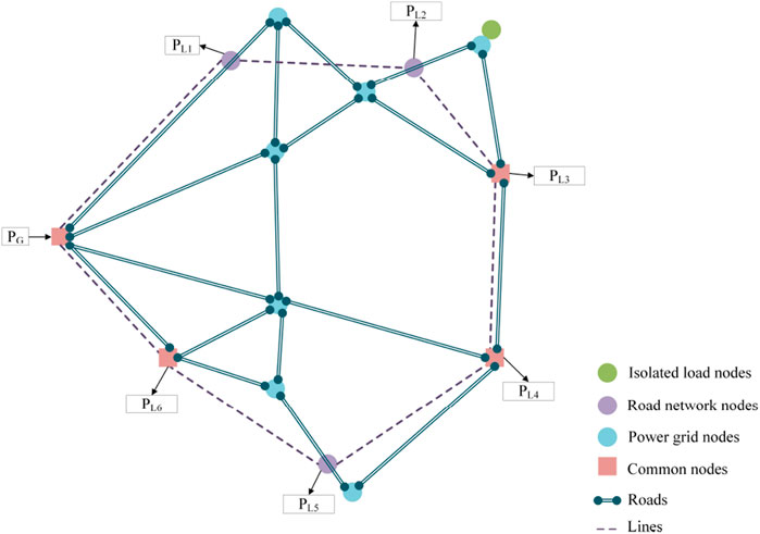
Figure 1. Power grid and road network topology under normal operating conditions.

2.1 Post-disaster scenario

Taking the damage to Weizhou Island’s power grid and road network caused by Typhoon Rammasun as an example, the post-disaster scenario on the island is specifically analyzed and described as follows (Author Anonymous, 2014):

1) Power Grid. The main transmission line network is the foundation for transmitting large capacities of electricity. The collapse of utility poles and disconnection of power lines will prevent electricity from power plants from being delivered to the user side in a timely manner. Therefore, the primary task of transmission network restoration is the reconstruction of the main grid. After Typhoon Rammasun, Weizhou Island’s power facilities suffered unprecedented damage. According to statistics, a total of 773 utility poles collapsed, and all 32 power supply areas (or distribution substations) were paralyz ed.

2) Road Network. Unlike the power grid, the main impact of the typhoon on roads was extensive road surface flooding and traffic obstruction caused by trees uprooted (or broken) by strong winds along roadsides. After one and a half days of repair, road traffic was restored.

3) Power Generation. The maximum power supply capacity of CNOOC (China National Offshore Oil Corporation) Weizhou Island Terminal Processing Plant is 12 MW. Weizhou Island’s peak load reaches 11 MW, and the island’s power supply and demand are basically balanced. However, due to extensive line damage caused by the typhoon’s passage, transmission channels were blocked, preventing timely power delivery and leading to power curtailment (or stranded power/generation congestion) on the generation side.

4) Users. As Weizhou Island’s power system was completely paralyzed, the user side experienced a continuous power outage. All important load nodes on Weizhou Island have backup diesel generators for emergency power supply, but due to limited capacity, they can only meet short-term power demand.

After the disaster, some transmission lines in the distribution network were damaged, and the power flow in the damaged transmission lines became 0. Some roads in the road network were damaged and impassable. The post-disaster coupled network topology is shown in Figure 2, where red indicates damaged roads (or transmission lines). Out of 18 roads, 9 were damaged, numbered 3, 4, 5, 6, 10, 11, 12, 15, and 17. Out of 7 transmission lines, 4 were damaged, numbered 2, 4, 5, and 7. This also caused the power flow in transmission line 6 to drop to 0, and loads 2, 3, 4, 5, 6, and 7 were all cut off from power.

Figure 2

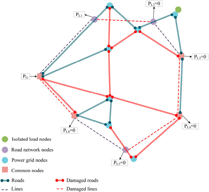
Figure 2. Distribution network road-network topology after disaster.

The road network contains a total of r roads. Depending on the damage situation of each road, the time required from the start of repair to the restoration of traffic on a road is defined as its repair time. The relationship between the required repair time for r roads, $\mathrm{T}{\mathrm{R}}_{\text{re}\left(r\times 1\right)}$, the repair start time ${\text{TR}}_{\text{res}\left(r\times 1\right)}$, and the repair completion time ${\text{TR}}_{\text{ref}\left(r\times 1\right)}$ is shown in Equation 1:

$\mathrm{T}{\mathrm{R}}_{\text{re}\left(r\times 1\right)}={\text{TR}}_{\text{ref}\left(r\times 1\right)}-{\text{TR}}_{\text{res}\left(r\times 1\right)}(1)$

Based on node locations, the transmission circuits are divided into l transmission lines. The fault types in the power grid include transformer damage, underground cable breaks, damage to overhead lines and towers, and line switch failures. Considering all fault types uniformly, the total time required from the start of repair of a line until the load nodes connected to it have their power supply restored is defined as the repair time for that line. The relationship between the required repair time for l transmission lines, ${\text{TL}}_{\text{re}\left(l\times 1\right)}$, the transmission line repair start time ${\text{TL}}_{\text{res}\left(l\times 1\right)}$, and the repair completion time ${\text{TL}}_{\text{ref}\left(l\times 1\right)}$ is shown in Equation 2:

${\text{TL}}_{\text{re}\left(l\times 1\right)}={\text{TL}}_{\text{ref}\left(l\times 1\right)}-{\text{TL}}_{\text{res}\left(l\times 1\right)}(2)$

A repair time of 0 indicates that the road or transmission line is undamaged and does not require repair; roads or transmission lines with a repair time greater than 0 all require repair. All repair times are finite values. Each road or transmission line requiring repair corresponds to a repair task. When transmission lines and roads overlap, if both the road and the transmission line are damaged simultaneously, the road must be repaired first, followed by the transmission line.

The varying damage conditions and repair times for different roads and transmission lines can fully reflect the type and severity of the disaster. Disasters like typhoons and ice storms typically have a lesser impact on roads, resulting in few damaged roads and short repair times, while power grid restoration requires a longer period. Conversely, disasters such as earthquakes and wars cause significant damage to both power and road networks. Generally, the higher the disaster level, the more severe the damage to both the road network and the power grid.

The dynamic interaction between the power grid and the road network is the core of coordinated repair, the dynamic interaction process is shown in Figure 3, and its process is manifested in a three-stage closed loop:

1) Road repair first: Post-disaster, road damage obstructs the passage of repair crews and the dispatch routes for MES. Road repair is the foundation for all subsequent work. Only when roads are passable can transmission line repair crews reach fault locations, and MES units can be transferred via the road network to off-grid load nodes, creating conditions for subsequent energy dispatch.

2) Dynamic resource release: Road repair triggers a dual resource release effect. First is the activation of repair resources: repair crews can travel along repaired roads to reach transmission fault points and initiate power restoration. Second is the dispatch of energy resources: MES units are transferred via the road network to off-grid nodes, constructing a temporary power supply network and alleviating power shortages for critical loads.

3) Power supply mode switching: After transmission lines are repaired, load nodes switch to main grid power supply, and the MES resources previously occupied are released. These MES units can then be redispatched to off-grid nodes in other unrepaired areas, forming a resource circulation support mechanism. This process maximizes the utilization of limited MES capacity while reducing the cumulative energy not supplied due to waiting for power restoration, ultimately achieving a coordinated optimization of minimizing both the full network power restoration time and the energy not supplied.

Figure 3

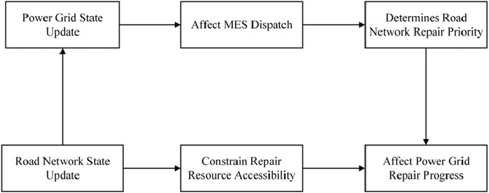
Figure 3. Flowchart of the dynamic interaction process between the power grid and the road network.

2.2 Joint restoration model for power supply based on coupled networks

2.2.1 Post-disaster power supply modes

2.2.1.1 MES power supply network

Available number of MES units and charging piles. At $N_1$ road nodes, there are a certain number of MES units, and at $N_2$ power grid nodes, there are a certain number of charging piles.

The initial number of MES units at each road network node is recorded in Equation 3:

${\mathrm{N}}_{\mathrm{r}-\text{mes}}={\left({\text{nn}}_i,{\mathrm{n}}_{\text{rmes}i}\right)}_{{\mathrm{N}}_1\times 1}i=1,2,\cdots ,N_1(3)$

where ${\text{nn}}_i$ is the road network node ID, ${\mathrm{n}}_{\text{rmesi}}$ is the number of MES units at node ${\text{nn}}_{\mathrm{i}}$.

During the restoration process, MES units can charge and discharge at connected network nodes. The number of MES units at each connected network node is recorded in Equation 4:

${\mathrm{N}}_{\text{rg}-\text{mes}}=\left({\text{nn}}_i,{\mathrm{n}}_{\text{rgmes}i}\right){\mathrm{N}}_2\times 2i=1,2,\cdots ,{\mathrm{N}}_2(4)$

where ${\text{nn}}_i$ is the connected network node ID, and ${\mathrm{n}}_{\text{rgmes}i}$ is the number of MES units connected at node ${\text{nn}}_i$.

During the restoration process, MES units can supply power to off-grid load nodes. The number of MES units at each off-grid load node is recorded in Equation 5:

${\mathrm{N}}_{\text{ro}-\text{mes}}={\left({\text{nn}}_i,{\mathrm{n}}_{\text{romes}i}\right)}_{\left({\mathrm{N}}_1-{\mathrm{N}}_2\right)\times 2}i=1,2,\cdots ,{\mathrm{N}}_1-{\mathrm{N}}_2(5)$

where ${\text{nn}}_i$ is the off-grid load node ID, and ${\mathrm{n}}_{\text{romesi}}$ is the number of MES units connected at node ${\text{nn}}_i$.

The adjacency matrix is determined by the actual geographical locations of the nodes and their connectivity sets. The location and charge/discharge state of MES units are determined according to the model’s evolution rules. MES units can charge/discharge at the load node of their current location and can also be moved to neighboring nodes to charge/discharge. Initially, if a load node is not connected to any other nodes, it is considered an isolated load node (or a load node with no neighbors). In this case, MES units within this node’s area can supply power to the load but cannot interact with the outside world, and the MES units cannot be recharged. When roads are restored, the node’s connectivity set is updated, the node can connect with other nodes, and the MES units regain their transfer capability.

2.2.1.2 Power grid supply mode

The power source is connected to load nodes via overhead lines/cables. By repairing transmission lines, load nodes are reconnected to the power source nodes, and users at these load nodes can have their power supply restored. The process of repairing transmission lines is a process of increasing the number of connected nodes and decreasing the number of off-grid nodes. According to the definition of node 1, the first row (or column) of the transmission line connectivity set CL represents the connectivity set for node 1, which is shown in Equation 6:

${\text{CL}}_1={\left({\mathit{cl}}_{1j}\right)}_{1\times \mathrm{N}}j=1,2,\cdots \mathrm{N}(6)$

The set of power grid nodes that can be supplied via transmission lines is shown in Equation 7:

${\mathrm{N}}_{\text{re}-\text{line}}=\left(n_j\right)n_j\in {\text{CL}}_1(7)$

2.2.2 Task allocation model

Assuming that the efficiency of repair crews is the same, and fault types are considered equivalent to a single type, there are g road repair crews to complete x road repair tasks, and h line repair crews to complete y line repair tasks. Under actual conditions, the number of repair crews in post-disaster fault scenarios is typically less than the number of repair tasks; therefore, this chapter only considers the cases where g < x and h < y.

1) The task allocation functions for road and transmission line repairs are shown in Equations 8, 9:

${\mathrm{R}}_{\mathrm{G}-\mathrm{X}}\left(i_1,j_1\right)=\left\{\begin{array}{l}1,\text{assign\hspace{0.17em}fault\hspace{0.17em}task\hspace{0.17em}}{x}_i\text{\hspace{0.17em}to\hspace{0.17em}repair\hspace{0.17em}crew\hspace{0.17em}}{\mathrm{G}}_j\\ 0,\text{else}\end{array}\right.\begin{array}{c}{i}_1=1,2,\cdots ,x\\ j_1=1,2,\cdots ,g\end{array}(8)$

${\mathrm{R}}_{\mathrm{H}-\mathrm{Y}}\left(i_2,j_2\right)=\left\{\begin{array}{l}1,\text{assign\hspace{0.17em}fault\hspace{0.17em}task\hspace{0.17em}}{y}_i\text{\hspace{0.17em}to\hspace{0.17em}repair\hspace{0.17em}crew\hspace{0.17em}}{\mathrm{H}}_j\\ 0,\text{else}\end{array}\right.\begin{array}{c}{i}_2=1,2,\cdots ,y\\ j_2=1,2,\cdots ,h\end{array}(9)$

2) The overall repair task allocation vector is shown in Equation 10:

$\mathrm{R}={\left[\begin{array}{cc}{\mathrm{R}}_{\mathrm{G}-\mathrm{X}}& 0\\ 0& {\mathrm{R}}_{\mathrm{H}-\mathrm{Y}}\end{array}\right]}_{\left(x+y,g+h\right)}(10)$

The overall repair process is divided into t₂ time periods. Then, the real-time task allocation vectors for road repair and transmission line repair in the k-th time period are RTG_k and RTH_k, as shown in Equations 11, 12:

${\text{RTG}}_K\left(i\right)=jk=1,2,\cdots ,t_2;i=1,2,\cdots ,g;j\in \left[1,x\right](11)$

${\text{RTG}}_K\left(m\right)=nk=1,2,\cdots ,t_2;m=1,2,\cdots ,h;j\in \left[1,y\right](12)$

The overall real-time task allocation vector is shown in Equation 13:

${\mathrm{R}}_t={\left[\begin{array}{cc}\text{RTG}& \text{RTH}\end{array}\right]}_{\left(g+h\right)}(13)$

2.3 Introduction to cellular automata

To address the dynamic balancing problem of power supply for isolated island loads using MES, a cellular automaton model can be adopted. The area where load nodes are located is considered as the cellular space. Each load node acts as a cell with a different load level and is equipped with DG and energy storage batteries matching the total load of the cell. The power supply state of a cell is closely related to the spatio-temporal distribution of MES units within the cellular space. A cellular automaton consists of numerous cells, and its overall behavior is an emergent property of the individual evolutionary behaviors of these cells. These cells hold equal status. The load nodes on Weizhou Island are numerous, discretely distributed, and have fixed locations, making them analogous to cellular units. The varying electricity demands of each load node represent different states of the cells.

Simultaneously, a model combining Agents with cellular automata is introduced. The autonomous learning and decision-making capabilities of Agents enable them to adjust their behavior according to environmental changes, aligning well with the discrete and distributed characteristics of cellular automata. The transferable nature of MES is similar to that of Agents, and their energy levels and charging/discharging states can serve as the basis for Agent state transitions. Cellular automata, through the setting of local rules and constraints, achieve self-organized decentralized control. This effectively handles the coupled relationships of complex spatio-temporal data and accelerates the power supply restoration of the distribution network after a disaster.

2.3.1 Cell indicators

2.3.1.1 Load energy demand

For ease of calculation, the discharge power of MES at the load is simplified. Assuming the average power of load node j from time t to t+∆t is $P_{lj}\left(t\right)$, then the energy demand of the load node during this time period $\Delta {\mathrm{E}}_{Lj}\left(t\right)$ which is shown in Equation 14:

$\Delta E_{Lj}\left(t\right)=P_{lj}\left(t\right)·\Delta t(14)$

2.3.1.2 Energy change due to transfer

The change in cell energy due to the movement of MES units (in and out) can be expressed as Equation 15:

$∆Q_j\left(t\right)={\displaystyle \sum _{k=1}^{N_j}}{\displaystyle \sum _{p=1}^{A_{jk}}}\left[E_{0P}{SOC}_p\left(t\right)-L_{jk}\right]-{\displaystyle \sum _{k=1}^{{\mathrm{N}}_{\mathrm{j}}}}{\displaystyle \sum _{p=1}^{A_{kj}}}\left[{\mathrm{E}}_{0p}{SOC}_q\left(t\right)\right](15)$

Where $A_{jk}$ represents the number of Agents moving from cell k to cell j in each time interval, ${\mathrm{N}}_{\mathrm{j}}$ represents the number of neighboring cells of cell j, $L_{jk}$ represents the energy loss during the movement of an Agent from cell k to cell j, $E_0$ is the battery capacity of the MES unit, p and q are the MES unit IDs, ${SOC}_p\left(t\right)$ represents the state of charge of MES p at time t, respectively.

2.3.1.3 Renewable energy output

Referring to Load Energy Demand, assuming the average output power of renewable energy in cell j from time t to t+∆t is $P_{gj}\left(t\right)$, then the renewable energy generation $∆E_{Gj}$ during this time period is as shown in Equation 16:

$∆E_{Gj}\left(t\right)=P_{gj}\left(t\right)·∆t(16)$

2.3.1.4 Cell energy

Cell energy is the available energy of a cell at the current time, including the available capacity of stationary energy storage (SES) and MES. Cell energy less than or equal to 0 means that the node has insufficient power at the current moment, and users experience a power outage. Therefore, cell energy can reflect the user’s outage situation, including outage duration and frequency.

As shown in Figure 4, the change in cell energy is mainly affected by three factors: ① decrease in cell energy due to load demand; ② energy change due to Agents moving in or out; ③ increase in cell energy due to renewable energy output. Therefore, the recursive formula for cell energy $E_j$ can be expressed as Equation 17 (taking cell j as an example, the same applies below):

$E_j\left(t+∆t\right)=E_j\left(t\right)+∆Q_j\left(t\right)+∆E_{Gj}\left(t\right)-∆E_{Lj}\left(t\right)(17)$

Figure 4

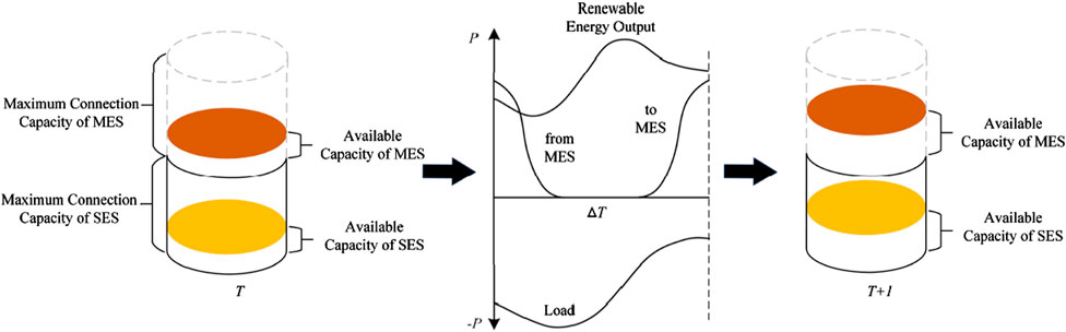
Figure 4. Process chart of cell energy change.

2.3.1.5 Cell activity

The actual physical meaning of cell activity is the power supply adequacy of the load node, characterized by the cell’s relative surplus energy. Cell surplus energy $E_r$ is the difference between the sum of the current energy storage capacity and the renewable energy output in the next time period, and the load energy demand, when the cell does not exchange energy with the outside world via MES, which is shown in Equation 18:

$E_{rj}\left(t\right)=E_j\left(t\right)+∆E_{Gj}\left(t\right)-∆E_{Lj}\left(t\right)(18)$

To improve the rationality of MES transfer decisions, referencing the concept of relative error, the cell relative surplus energy $\delta E_{rj}\left(t\right)$ is defined as the ratio of cell surplus energy to load energy demand, which is shown in Equation 19:

$\delta E_{rj}\left(t\right)=\frac{E_{rj}\left(t\right)}{∆E_{Lj}\left(t\right)}(19)$

2.3.2 MES dispatch method based on cellular automata

The state update time interval is taken as the maximum of the travel time and the load sampling time, as shown in Equation 20:

$∆t=\max \left\{\frac{{\mathrm{s}}_1}{\mathrm{v}},\frac{{\mathrm{s}}_2}{\mathrm{v}},\cdots ,\frac{{\mathrm{s}}_{\mathrm{i}}}{\mathrm{v}},15\min \right\}(20)$

where the route segment distance between adjacent cells is denoted as ${\mathrm{s}}_{\mathrm{i}}$, and there are a total of m routes; it is assumed that all Agents move at a fixed speed v.

The specific rules are as follows:

1) If an Agent’s remaining SOC does not exceed the reserved energy $E_{\text{stop}}$, it sends a charging request (or power intake request) to the control center and gradually withdraws from the power supply network within the next time interval.

2) If an Agent is in a charging state and has reached full charge, it sends a dispatch request (or power delivery request) to the control center and gradually withdraws from the power supply network within the next time interval.

3) If an Agent’s remaining SOC is higher than $E_{stop}$, and the energy level of the cell it is in satisfies $E\le \left(1+\delta \right)\overline{E}$ (where $E_{\text{stop}}$ represents the average energy level within the cell’s neighborhood, and $\delta$ represents the buffer threshold, tuned based on expert experience), then the Agent’s state remains unchanged.

4) If cell i, where an Agent is located, receives a transfer-out command from cell j, and its remaining SOC is the lowest among all Agents in cell i, then in the next time period, it withdraws from cell i and moves to connect to cell j.

Furthermore, when the activity of a cell in the network drops below a warning threshold, the control center dispatches a fully charged Agent to connect to that cell.

3 Objective function and constraints

3.1 Objective function

Considering the more rational utilization of the MES power supply network for emergency power supply and the impact of the importance of different load nodes on decision-making, this paper takes a weighted sum of unserved energy, related to the importance of each load node, as the optimization objective.

Loads within the network are classified into three levels based on importance (Liu, 2017):

Level 1 loads are defined as those for which power outages are absolutely not permissible, such as military bases, critical communication hubs, major transportation hubs, and administrative centers.

Level 2 loads are defined as those for which power outages would cause significant political and economic losses, such as industrial and commercial loads, communication hubs, transportation hubs, and important residential loads.

The remaining loads in the distribution network are defined as Level 3 loads.

Minimizing the sum of the products of the unserved energy at all load nodes and their respective importance weights allows the optimization results to be biased by node importance; the higher the importance of a load node, the more the model tends to yield a result with less unserved energy for that node (Lan, 2016). Accordingly, the objective function is designed as Equation 21:

$\min F={\int }_{i=1}^{{\mathrm{N}}_2-1}{\mathrm{u}}_i·{\mathrm{W}}_{\text{loss}-i}(21)$

where ${\mathrm{u}}_i$ represents the load priority weight of load node i; $W_{\text{loss}-i}$ is the actual unserved energy at load node i, equal to the difference between energy demand and actual energy supplied. The energy demand of a load node can be calculated from the total grid restoration time and the load node power. The actual energy supplied consists of energy supplied by the power grid and energy supplied by the MES network.

The total grid restoration time $T_f$ is equal to the total repair time of the scheme, i.e., the difference between the latest transmission line repair completion time and the earliest transmission line repair start time, as shown in Equation 22:

$T_f=\max \left\{{\text{TL}}_{\text{ref}i}\right\}-\min \left\{\mathrm{T}{\mathrm{L}}_{\text{res}j}\right\}i=1,2,\cdots ,l(22)$

The sum of electricity demand in each time period yields the total electricity demand $W_{\mathrm{F}-i}$ of load node i during the entire restoration process, as shown in Equation 23:

$W_{\mathrm{F}-i}={\displaystyle \sum _{j=1}^{t_2}}{\overline{P}}_{\mathrm{F}ij}{T}_j(23)$

where $T_j$ is the duration of time period j, and ${\overline{P}}_{\mathrm{F}ij}$ is the average load power of node i in time period j.

The number of grid-connected nodes changes dynamically during the restoration process. First, based on the set of grid nodes Nre-line supplied by transmission lines, the 0–1 time-period grid connectivity matrix LP is obtained, which determines whether a load node is connected to the grid, LP is shown in Equation 24:

$\begin{array}{l}\text{LP}={\left(\mathit{l}{\mathit{p}}_{ij}\right)}_{\left({\mathrm{N}}_2-1\right)\times t_2}\\ \mathit{l}{\mathit{p}}_{\mathrm{ij}}=\left\{\begin{array}{l}1\text{\hspace{1em}Load\hspace{0.17em}\hspace{0.17em}\hspace{0.17em}node\hspace{0.17em}\hspace{0.17em}\hspace{0.17em}}i\text{\hspace{0.17em}\hspace{0.17em}\hspace{0.17em}is\hspace{0.17em}\hspace{0.17em}\hspace{0.17em}grid}-\text{connected\hspace{0.17em}\hspace{0.17em}\hspace{0.17em}in\hspace{0.17em}\hspace{0.17em}\hspace{0.17em}period\hspace{0.17em}\hspace{0.17em}\hspace{0.17em}}ji=1,2,\cdots ,{\mathrm{N}}_2-1\\ 0\text{\hspace{1em}Load\hspace{0.17em}\hspace{0.17em}\hspace{0.17em}node\hspace{0.17em}\hspace{0.17em}\hspace{0.17em}}i\text{\hspace{0.17em}\hspace{0.17em}\hspace{0.17em}is\hspace{0.17em}\hspace{0.17em}\hspace{0.17em}off}-\text{grid\hspace{0.17em}\hspace{0.17em}\hspace{0.17em}in\hspace{0.17em}\hspace{0.17em}\hspace{0.17em}period\hspace{0.17em}\hspace{0.17em}\hspace{0.17em}}jj=1,2,\cdots ,t_2\end{array}\right.\end{array}(24)$

The time-period average grid supply power for load node i is ${\overline{P}}_{Gi}$, which in shown in Equation 25:

${\overline{P}}_{Gi}=\left[{\overline{P}}_{Gi1}{\overline{P}}_{Gi2}\cdots {\overline{P}}_{Gi{t}_2}\right](25)$

The time-period grid energy supplied to load node i is shown in Equation 26:

$\begin{array}{l}{\mathrm{W}}_{gi}={\left(\mathit{w}{\mathit{g}}_{ij}\right)}_{t_2}\\ {\mathit{wg}}_{ij}=l{p}_{ij}{\overline{P}}_{Gij}{T}_{j}i=1,2,\cdots ,N_2-1;j=1,2,\cdots ,t_2\end{array}(26)$

Then, summing the energy supplied over all time periods yields the total grid energy supplied to load node i, as shown in Equation 27:

$W_{\mathrm{G}-i}={\displaystyle \sum _{i=1}^{{\mathrm{N}}_2-1}}{\mathrm{u}}_i·W_{loss-i}(27)$

Similarly, the 0–1 time-period MES network supply matrix is determined, indicating whether load node i is supplied by MES (i represents the load node number), which is shown in Equation 28:

$\begin{array}{l}\text{LM}={\left(\mathit{l}{\mathit{m}}_{ij}\right)}_{\left({\mathrm{N}}_2-1\right)\times t_2}\\ \mathit{l}{\mathit{m}}_{ij}=\left\{\begin{array}{l}1,\text{Powered\hspace{0.17em}\hspace{0.17em}\hspace{0.17em}by\hspace{0.17em}\hspace{0.17em}\hspace{0.17em}MES\hspace{0.17em}\hspace{0.17em}\hspace{0.17em}in\hspace{0.17em}\hspace{0.17em}\hspace{0.17em}period\hspace{0.17em}\hspace{0.17em}\hspace{0.17em}}ji=1,2,\cdots ,{\mathrm{N}}_2-1\\ 0,\text{Not\hspace{0.17em}\hspace{0.17em}\hspace{0.17em}powered\hspace{0.17em}\hspace{0.17em}\hspace{0.17em}by\hspace{0.17em}\hspace{0.17em}\hspace{0.17em}MES\hspace{0.17em}\hspace{0.17em}\hspace{0.17em}in\hspace{0.17em}\hspace{0.17em}\hspace{0.17em}period\hspace{0.17em}\hspace{0.17em}\hspace{0.17em}}jj=1,2,\cdots ,t_2\end{array}\right.\end{array}(28)$

The time-period average MES network supply power for load node i is ${\overline{P}}_{Mi}$, which is shown in Equation 29:

${\overline{P}}_{Mi}=\left[\begin{array}{cccc}{\overline{P}}_{Mi1}& {\overline{P}}_{Mi2}& \cdots & {\overline{P}}_{Mi{t}_2}\end{array}\right](29)$

The time-period MES network energy supplied to load node i is shown in Equation 30:

$\begin{array}{l}{\mathrm{W}}_{mi}={\left(\mathit{w}{\mathit{m}}_{\mathit{ij}}\right)}_{t_2}\\ w{m}_{ij}=l{m}_{ij}{\overline{P}}_{Mij}{T}_j\mathrm{i}=1,2,\cdots {\mathrm{N}}_2-1;j=1,2,\cdots ,t_2\end{array}(30)$

Then, summing over all time periods yields the total MES energy supplied to load node i, as shown in Equation 31:

$W_{\mathrm{M}-i}={\displaystyle \sum _{j=1}^{t_2}}w{m}_{ij}(31)$

The actual unserved energy (or electricity shortage) for load node i is shown in Equation 32:

$W_{\text{loss}-i}=W_{\mathrm{F}-i}-\left(W_{\mathrm{G}-i}+W_{\mathrm{M}-i}\right)(32)$

3.2 Constraints

In the road network-power grid coupled network model, three aspects of constraints need to be considered: power grid constraints, road network constraints, and repair task logic constraints. Among these, power grid constraints include branch power flow constraints, node voltage constraints (Lu et al., 2011), and charging pile quantity constraints. Accessibility constraints include repair transportation accessibility constraints and repair crew capability constraints. Furthermore, during the operation of MES, its own constraints also need to be considered.

3.2.1 Power grid constraints

1) Branch power flow constraint. After line repair, the power transmitted by each transmission line should satisfy Equation 33:

$\left|P_i\right|\le {\mathrm{P}}_{imax}(33)$

Where $P_i$ is the power flowing through transmission line i, and ${\mathrm{P}}_{i\max }$ is the maximum power limit of transmission line i.

2) Node voltage constraint. After line repair, the voltage at each node should satisfy Equation 34:

${\mathrm{U}}_{\min }\le U\le {\mathrm{U}}_{\max }(34)$

Where ${\mathrm{U}}_{\max }$ and ${\mathrm{U}}_{\min }$ are the upper and lower limits of the node voltage, respectively.

3) Charging pile quantity constraint. Due to the varying number of charging piles at each node, the number of connected MES units is limited by the number of charging piles. In the N+1 transfer mode, the number of MES units connected at node nn should be at least one less than the number of charging piles, which is shown in Equation 35:

$n_{rgmes}\left(nn\right)\le n_{cpi}\left(nn\right)-1(35)$

3.2.2 Road network constraints

Since repair tools, materials, and personnel need to be transported by vehicles, the roads or transmission lines to be repaired must be connectable to the workstation via roads. Combining with the road connectivity set, the workstation is located at the node numbered ${\mathrm{N}}_{\text{WS}}$. Road nodes connected to node N_WS are accessible nodes for the repair crew, i.e., the N_WS-th row elements of the road connectivity set. Based on this, the repair accessibility matrix is defined as Equation 36:

$\mathrm{C}{\mathrm{R}}_{{\mathrm{N}}_{WS}j}={\left(c{r}_{{\mathrm{N}}_{WS}j}\right)}_{N_1}j=1,2,\cdots ,N_1(36)$

In the repair accessibility matrix, if an element is “1″, it means the node corresponding to that column is connected to the workstation and accessible to the repair crew; otherwise, it is not connected to the workstation, and the repair crew cannot reach it.

3.2.3 Repair task logic constraints

Some transmission lines are located on roads, or their repair materials and tools need to be transported to nearby roads. If these nearby roads are damaged, they must be repaired first before the transmission line repair work can begin. The repair logic matrix $\mathrm{L}{\mathrm{R}}_{\text{order}}\left(i,j\right)$ is defined as Equation 37:

$\mathrm{L}{\mathrm{R}}_{\text{order}}\left(i,j\right)=\left\{\begin{array}{l}1,\text{Line\hspace{0.17em}\hspace{0.17em}\hspace{0.17em}}i\text{\hspace{0.17em}\hspace{0.17em}\hspace{0.17em}can\hspace{0.17em}\hspace{0.17em}\hspace{0.17em}be\hspace{0.17em}\hspace{0.17em}\hspace{0.17em}repaired\hspace{0.17em}\hspace{0.17em}\hspace{0.17em}when\hspace{0.17em}\hspace{0.17em}\hspace{0.17em}road\hspace{0.17em}\hspace{0.17em}\hspace{0.17em}}j\text{\hspace{0.17em}\hspace{0.17em}\hspace{0.17em}is\hspace{0.17em}\hspace{0.17em}\hspace{0.17em}damaged\hspace{1em}}i=1,2,\cdots ,l\\ 0,\text{else\hspace{1em}}j=1,2,\cdots ,r\end{array}\right.(37)$

When an element in the repair logic matrix is “1″, the road repair corresponding to the column and the transmission line repair corresponding to the row do not interfere with each other. When an element is “0″, it indicates a logical dependency between the road and the transmission line, requiring the road to be repaired before the transmission line. Due to these constraints, unavoidable waiting times may occur during the repair process.

3.2.4 MES constraints

The SOC at the current time t, SOC(t), can be calculated by Equation 38 (Jeon et al., 2023):

${SOC}_i\left(t\right)=\left\{\begin{array}{c}{SOC}_i\left(t_0\right)+{\int }_t^{t_0}\frac{P_{\text{cha},i}{\eta }_{\text{cha},i}}{{\mathrm{E}}_{\text{bat},i}}\mathrm{d}t\\ {SOC}_i\left(t_0\right)+{\int }_t^{t_0}\frac{P_{\text{dis},i}{\mathrm{\eta }}_{\text{dis},i}}{{\mathrm{E}}_{\text{bat},i}}\mathrm{d}t\end{array}\right.(38)$

Where i is the MES unit number, $t_0$ is the time when the MES unit arrives at the charging/discharging location, $P_{\text{cha}}$ and $P_{\text{dis}}$ are the charging and discharging powers, respectively, ${\eta }_{\text{cha}}$ and ${\eta }_{\text{dis}}$ are the charging and discharging efficiencies, respectively, and ${\mathrm{E}}_{\text{bat}}$ is the nominal battery capacity.

The SOC at the initial stopping time $t_0$, $SOC\left(t_0\right)$, equals its SOC before travel minus the energy consumed during travel by the MES unit, and then minus the SOC change from previous charging/discharging actions, as shown in Equation 39:

${SOC}_i\left(t_0\right)=1-{\int }_t^{t_0}\frac{{\eta }_{\text{EV}}\overline{\mathrm{v}}}{{\mathrm{E}}_{\text{bat}}}dt-∆{SOC}_i(39)$

Where ${\eta }_{\text{EV}}$ represents the driving efficiency (i.e., energy consumption per kilometer), and $\overline{\mathrm{v}}$ is the average driving speed of MES.

Maximum power constraint of MES is shown in Equation 40:

$\left\{\begin{array}{c}{P}_{\text{cha},i}\left(t\right)\le P_{\text{cha},i,\max }\\ P_{\text{dis},i}\left(t\right)\le P_{\text{dis},i,\max }\end{array}\right.(40)$

Where $P_{\text{cha},i}\left(t\right)$ and $P_{\text{dis},i}\left(t\right)$ are the charging and discharging powers of MES unit i at time t, respectively; $P_{\text{cha},i,\max }$ and $P_{\text{dis},i,\max }$ are the maximum allowable charging and discharging powers of MES unit i, respectively.

Meanwhile, to avoid damage to the power battery’s cycle life due to overcharging or overdischarging, the SOC usually needs to be maintained within a certain range, which is shown in Equation 41:

${\text{SOC}}_{\text{down}}\le {SOC}_i\left(t\right)\le {\text{SOC}}_{\text{up}}(41)$

Where ${\text{SOC}}_{\text{up}}$ and ${\text{SOC}}_{\text{down}}$ are the highest and lowest SOC thresholds, respectively, that do not cause additional damage to the power battery’s service life.

Based on the power battery’s discharge lower limit, the available energy $E_i\left(t\right)$ of MES unit i at time t is defined in Equation 42:

$E_i\left(t\right)=\left[{SOC}_i\left(t\right)-{\text{SOC}}_{\text{down}}\right]E_{0i}(42)$

During the discharging process of the MES, the recursive formula for the SOC at each time step is shown in Equation 43:

$E_{0i}{SOC}_i\left(t+∆t\right)=E_{0i}{SOC}_i\left(t\right)P_{ei}\left(t\right)∆t(43)$

Where Δt is the dispatch time interval, $E_{0i}$ is the battery capacity of MES unit i, and $P_{ei}\left(t\right)$ is the discharging power of MES unit i at time t.

3.3 Solution process

Distribution networks are generally not large, and their grid structure is simple. Moreover, the repair problem studied in this chapter only considers the scenario of a single fault point on a single segment. Therefore, the optimization problem for the repair plan is not a complex non-convex problem and can be solved using an enumeration algorithm. However, during the repair process, due to the adoption of a hybrid power supply mode, the solution process, including network state updates, is relatively complex and needs to be elaborated upon. The solution process is shown in Figure 5, and the specific steps are as follows:

1) Initialize Network Parameters. This includes power grid parameters such as distribution network line numbers, power grid node numbers, transmission line power, and rated load power; road network parameters such as road network road numbers and road network node numbers; numbers of coupled nodes and common nodes; the number of MES units at each node; the number of charging piles at each node; the number of two types of repair crews, and the location of the workstation.

2) Initial Disaster Situation. Determine the damaged transmission line and road numbers; calculate the power supply status of each load node in the remaining network; calculate the number of available MES units at connected nodes.

3) Repair Task Confirmation. Based on the damage status of the power grid and road network, and the power supply status of load nodes, determine the transmission lines and roads that need repair. Assign the transmission lines and roads requiring repair as repair tasks, and evaluate the time required to complete each repair task.

4) Design Repair Plan. Initially set the repair task assignment vectors, including road repair task assignment vectors and transmission line repair task assignment vectors. Determine the piecewise function for repair time. According to the repair objectives and constraints, the repair plan should follow these principles:

① Prioritize the restoration of damaged roads that affect the transportation of repair materials and constrain line repair work.

② After the aforementioned roads are repaired, prioritize the restoration of roads required for the transfer of MES units.

③ Prioritize the restoration of damaged transmission lines that are closer to the power source node (referring to line distance, not spatial distance).

④ Since the work efficiency of repair crews is the same, different task assignments at the same time are equivalent; thus, only one such scheme is considered.

⑤ If it does not affect transmission line repair and MES movement, different road repair task assignments are equivalent; thus, only one such scheme is considered.

5) Network State Update. After each repair task is completed, the system is updated once. The updated data includes:

① Repair tasks completed in the current period and subsequent work tasks for the repair crews;

② Numbers of repaired transmission lines, connected node numbers, and numbers of repaired roads;

③ Changes in the quantity, location, and SOC of connected MES units; input/output power of MES units in the current period;

④ Average power supply and duration from the grid to each load node in the current period;

⑤ Node direct connection sets, connectivity sets, and cell neighbor matrix;

⑥ Combining the cell neighbor matrix and the proposed MES power supply network evolution rules, record the discharge power and duration of MES units at each load node.

6) When Network Update Ends, record the numbers of nodes experiencing outages in each stage; record the duration for which MES units supply power to each load node; record the duration for which the power grid supplies power to each load node.

7) After All Repair Tasks Are Completed, record the time required for full power restoration to the entire network.

8) Change the Repair Task Assignment Vector Based on the Enumeration Method. Return to step 5) until all possible assignment schemes have been enumerated.

9) Calculate the weighted sum of energy not supplied (ENS) for each scheme, and select the task assignment vector with the minimum weighted sum of ENS as the optimal repair plan.

Figure 5

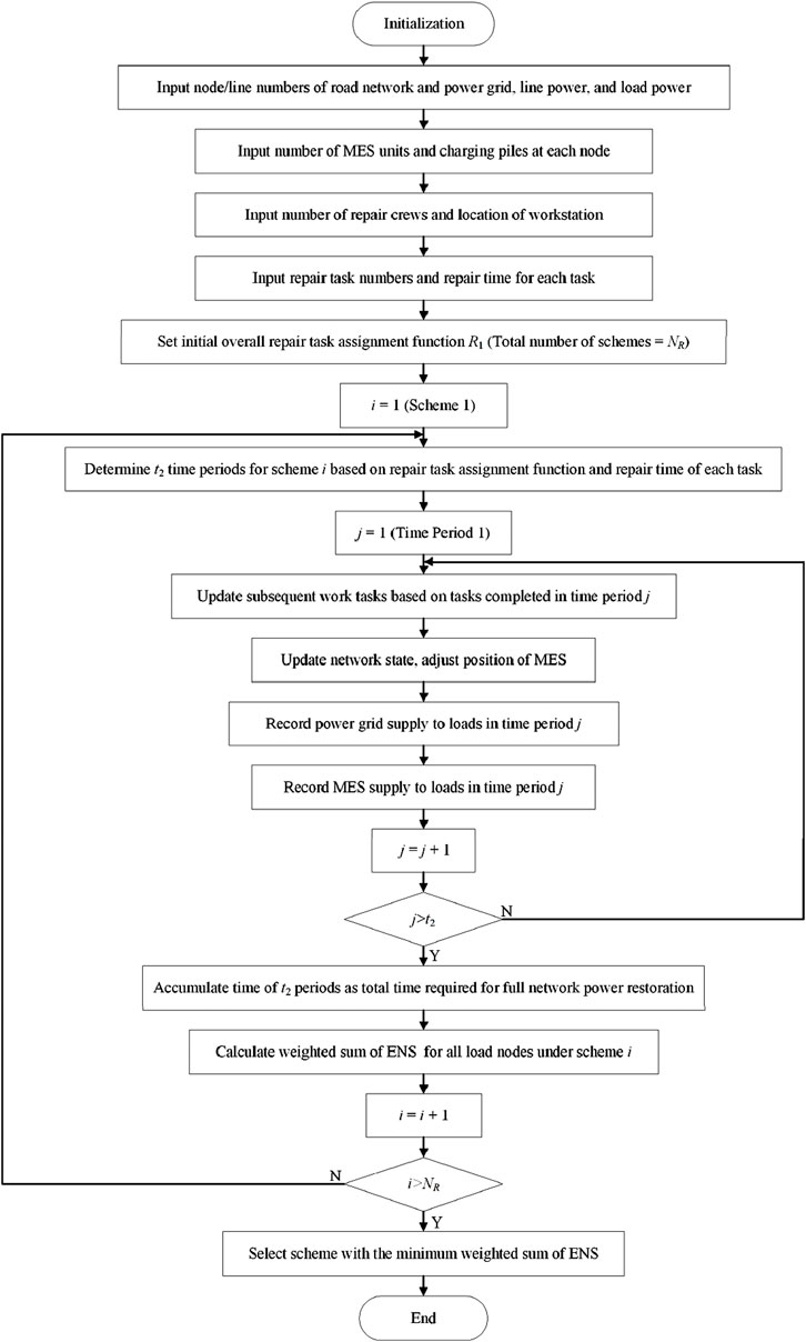
Figure 5. Solving process for emergency repair of ocean island microgrid based on hybrid power supply mode.

4 Case study analysis

4.1 Simulation scene

This paper takes the Weizhou Island road network-power grid scenario as an example to verify the effectiveness of the proposed repair strategy. The post-disaster coupled network topology is shown in Figure 6. Among them, the workstation is located at road node No. 1.

Figure 6

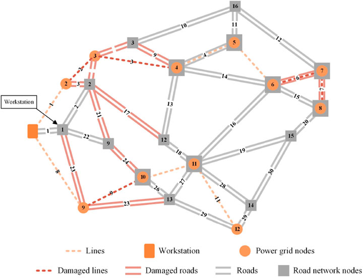
Figure 6. Topology map of post disaster coupling network in Weizhou Island.

Considering the particularity of the disaster scenario, to allocate electrical energy more systematically and scientifically, and to maximize the rational use of limited energy, this section assigns power to load nodes based on load type and population. The average power and weight coefficients of the load nodes are shown in Table 1. The diurnal load factor for different types of loads are shown in Figure 7.

Table 1

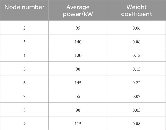
Table 1. Load node weight coefficient setting.

Figure 7

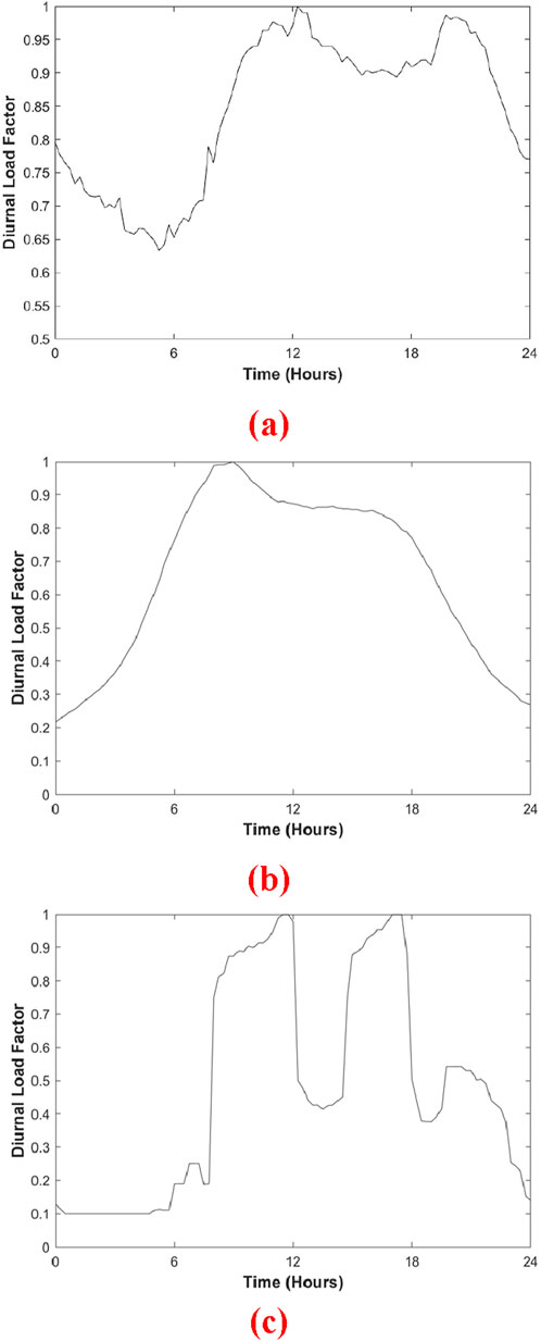
Figure 7. Daily load factor of different types of loads. (a) Load level 1. (b) Load level 2. (c) Load level 3.

Each node is equipped with distributed PV of a certain capacity. The weekly solar irradiance power density variation curve is shown in Figure 8. It can be seen that the solar irradiance power density is generally at its maximum around noon each day, and is typically zero at night (18:00–06:00 the next day).

Figure 8

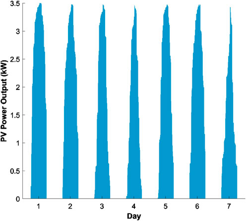
Figure 8. PV output curve.

4.2 Simulation parameter settings

Table 2 lists some parameter values for the coupled network, including: number of power grid nodes, number of lines, number of load nodes, and the numbers of power supply nodes and coupled nodes; number of road network nodes, and number of roads. Table 3 lists the number of available MES units at each load node. All MES units are of the same model, with an initial SOC of 0.5. Tables 4, 5 list the numbers of damaged roads and damaged lines, respectively, and the planned time quota for each repair task. The repair start date is Day 0, and the start time is 0:00. To simplify the case study, in the simulation, a uniform model is selected for both MES and SES. The specific technical parameters are shown in Table 6.

Table 2

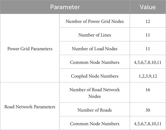
Table 2. Coupling network parameter settings.

Table 3

Table 3. The number of MES in each node area.

Table 4

Table 4. Time quota for rush rapiars.

Table 5

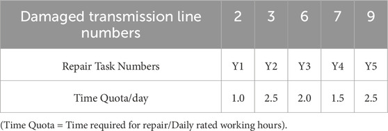
Table 5. Time quota for rush rapairs of transmission lines.

Table 6

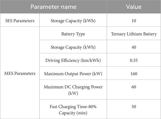
Table 6. Time quota for rush rapairs of transmission lines.

4.3 Simulation results analysis

4.3.1 Repair plan design

There are 2 road repair crews (G1, G2) and 2 line repair crews (H1, H2) on the island. According to the repair constraints and principles, a total of 7 task assignment schemes were designed. The task assignment for each scheme is shown in Table 7.

Table 7

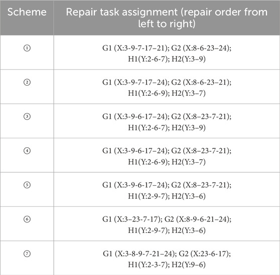
Table 7. Rush repair task allocation table.

Under each scheme, the construction time, waiting time, and total time for road repair and line repair are shown in Table 8. Among these, the total time for each repair crew includes the construction time for all repair tasks and the necessary waiting time between repairs due to repair task accessibility constraints and repair task logic constraints. Under different repair schemes, due to different repair sequences, the waiting times caused by repair constraints also differ; therefore, the total planned time for different schemes also varies. If all repair tasks proceed smoothly according to plan, the total time is the time required for full network power restoration. It should be noted that the unit “day” for repair time represents 12 h of working time. These 12 h can be divided into four periods: 6:00–9:00, 9:00–12:00, 13:00–16:00, and 16:00–19:00, with each period representing 0.25 days. However, when calculating supplied energy and energy not supplied, a day is still calculated as 24 h.

Table 8

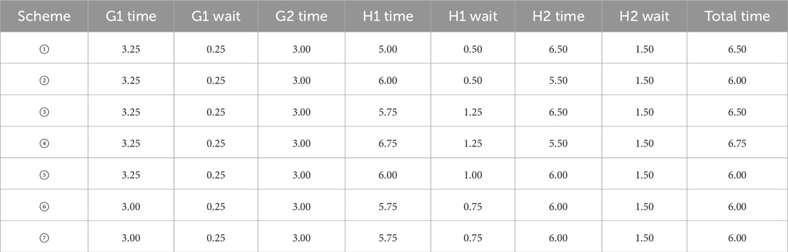
Table 8. Rush repair schedule.

Taking Scheme ① as an example, the start and completion times for each repair task are listed in Table 9. According to the end times of each task in the table, the entire repair process under this scheme is divided into 12 periods. 0 represents the start time, and the end times (in days) for each period are: 0.25, 0.50, 1.25, 1.50, 2.00, 2.75, 3.00, 3.25, 3.50, 4.00, 5.00, 6.50. The durations (in days) of the 12 periods are: 0.25, 0.25, 0.75, 0.25, 0.50, 0.75, 0.25, 0.25, 0.25, 0.50, 1.00, 1.50.

Table 9

Table 9. Timesharing of rush repair task.

The time-scaled activity-on-arrow network plan diagram for Scheme ① is shown in Figure 9. Nodes represent the start or end time of tasks, the horizontal projection length of solid arrow lines represents task duration, horizontal wavy lines represent waiting time, and dashed arrow lines represent logical relationships. As seen in the figure, the following logical relationships exist among the repair tasks: before repair task Y2 can begin, repair tasks X3 and X8 must be completed; before repair task Y6 can begin, repair task X6 must be completed; before repair task Y7 can begin, repair task X7 must be completed; before repair task Y9 can begin, repair task X23 must be completed.

Figure 9

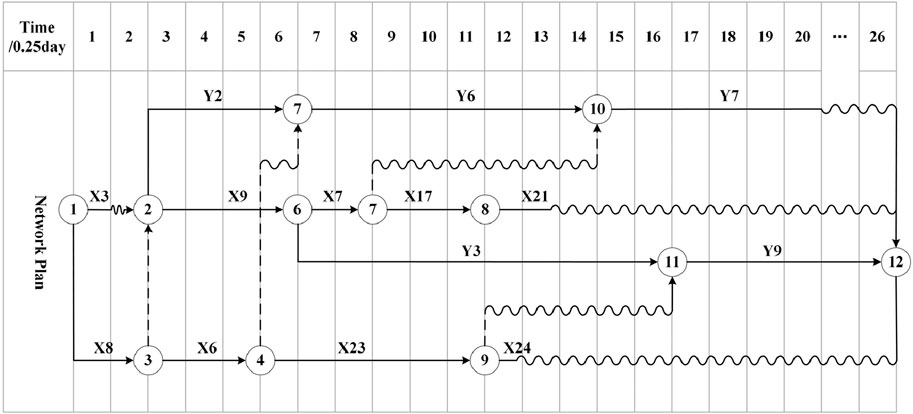
Figure 9. Network plan of double code time scale for rush repair task (plan ①).

4.3.2 Cell energy

Taking load node 9 as an example, when MES does not participate in the charging and discharging process of the load node, its energy curve is shown in Figure 10a; in the mobile energy storage power supply network, its energy curve is shown in Figure 9b.

Figure 10

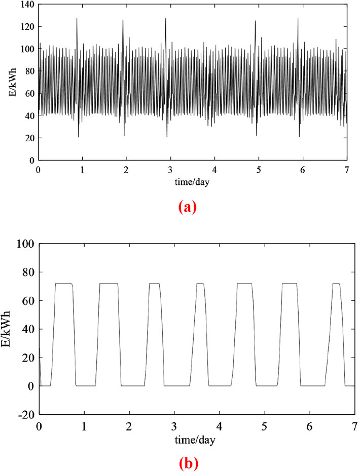
Figure 10. (a) Cell energy curve of load node 9 in the mobile energy storage power supply network. (b) Cell energy curve of load node 9 when MES does not participate in the load node charging and discharging process.

In the case shown in Figure 10a, the cell energy is equal to the available capacity of the SES. Since the influence of MES is not considered, the cell energy does not fluctuate frequently and exhibits a similar trend each day: during the daytime, PV power output is relatively large, and the available capacity of the SES continuously accumulates. However, due to the limitation of the SES capacity, when it accumulates to a certain point, the storage capacity remains at a fixed value, and the cell energy no longer increases. After the PV output drops to zero, users rely on the energy stored by the SES during the daytime for power supply; the cell energy continuously decreases until it drops to zero at a certain point, after which they remain in a power outage state. Examining the outage situation for all 11 load nodes, the average user outage time is 84.4 h, and the power supply reliability rate is only 49.1%. It can be seen that if the mobile energy storage power supply network is not adopted, user power supply reliability will be significantly reduced.

As seen in Figure 10b, the cell energy of each load node oscillates within a certain range. This is formed under the combined effects of MES transfer, output fluctuations, and load demand. Although the cell energy changes frequently, the cell energy of each load node remains greater than 0 throughout the entire process, and this conclusion holds for the other nodes as well. Therefore, in the current scenario, each load node never experiences a power outage, the average outage time is 0, and the power supply reliability rate of the MES network can reach 100%. It can be seen that when the quantity of MES is sufficient, the MES power supply network can effectively ensure the power supply reliability of isolated load nodes post-disaster.

4.3.3 Weighted sum of ENS

Combining the repair plan and power grid constraints, the grid supply time is calculated. Based on road network constraints, the operational status of MES units in the MES power supply network is simulated using Matlab. According to the output results, the time and output power for MES units supplying each load node are calculated. The weighted sum of ENS for all load nodes is calculated. Taking Scheme ① as an example, the grid-supplied energy, MES network-supplied energy, energy demand, and actual energy not supplied for each load node are shown in Figure 11. Figure 12 shows the weighted sum of ENS for each scheme.

Figure 11

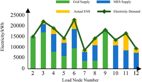
Figure 11. Power supply and power loss of each load node (example ①).

Figure 12

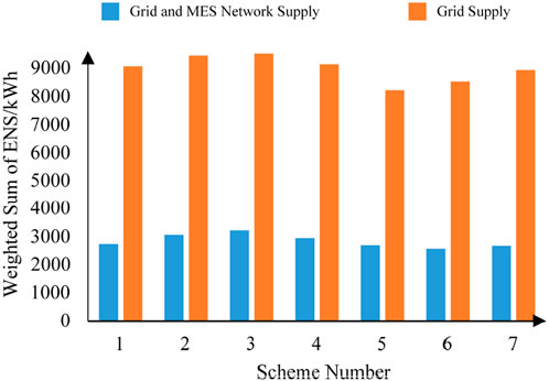
Figure 12. The power loss weight of each scheme.

As seen in Figure 11, load nodes 2 and 9 are powered by the grid throughout the entire repair process and do not require MES units. Therefore, the MES network-supplied energy at these nodes is 0, and the actual ENS is also 0. This is because the transmission lines between these nodes and the grid were not damaged and were connected to the power source node from the initial moment. The actual energy supplied to load nodes 3, 4, 5, 6, 7, and 8 consists of grid-supplied energy and MES network-supplied energy. During off-grid periods, these load nodes are powered by MES units, but due to limitations in the number of MES units and road accessibility constraints, not all load node demands can be fully met. After these load nodes are reconnected to the grid, they switch to grid power. Load nodes 10, 11, and 12 remain off-grid until full network power restoration, relying solely on MES units for power throughout the process. If the MES power supply network were not introduced, load nodes 10, 11, and 12 would remain in a state of power outage, and the ENS for load nodes 3, 4, 5, 6, 7, and 8 would also significantly increase. This demonstrates that introducing the MES power supply network can significantly improve the power supply situation for load nodes post-disaster.

As seen in Figure 12, under each scheme, the weighted sum of ENS when using both grid and MES network power supply modes is much smaller than relying solely on grid power. Therefore, introducing the MES power supply network plays an important role in load assurance. Scheme ⑥ is the optimal scheme. Without MES network power supply (relying only on the grid), the weighted sum of ENS is 8,513 kWh. When both modes are used, the weighted sum of ENS is only 2,551 kWh, a reduction of 70%. This shows that after using MES network auxiliary power supply, the weighted sum of ENS is significantly reduced, effectively alleviating power supply pressure during the repair period.

5 Conclusion

In summary, this paper, based on the MES model, the coupled network model, and the MES power supply network model, establishes model assumptions by considering actual post-disaster scenarios in distribution networks. After fully considering constraints related to the power grid, road network, and repair task logic, the paper proposes utilizing two power supply modes—the power grid and the MES power supply network—to provide power support for load nodes during the post-disaster repair period. Work plans for road repair and power system repair are then comprehensively arranged with the objective of minimizing the weighted sum of energy not supplied for all load nodes. The simulation results demonstrate that the proposed strategy can significantly improve the power supply situation for load nodes after a disaster and alleviate the challenge of power shortages during the repair period.

Data availability statement

The raw data supporting the conclusions of this article will be made available by the authors, without undue reservation.

Author contributions

SZ: Resources, Methodology, Writing – original draft, Writing – review and editing, Formal Analysis. YC: Writing – original draft, Resources, Project administration, Writing – review and editing, Funding acquisition. YL: Project administration, Writing – original draft, Writing – review and editing, Methodology. YH: Writing – review and editing, Conceptualization, Writing – original draft, Visualization. ZL: Writing – review and editing, Investigation, Writing – original draft, Supervision, Data curation, Validation, Project administration. RL: Conceptualization, Formal Analysis, Writing – review and editing, Software, Writing – original draft.

Funding

The author(s) declare that financial support was received for the research and/or publication of this article. This research was funded by the Science and Technology Research Program of Guangdong Power Grid Guangzhou Power Supply Bureau (No. 030108KK52222008).

Acknowledgments

The authors sincerely acknowledge the contribution of all individuals, reviewers, and editors for their contribution towards the production of this manuscript.

Conflict of interest

Authors SZ, YC, YL were employed by Guangdong Power Grid Guangzhou Power Supply Bureau.

The remaining authors declare that the research was conducted in the absence of any commercial or financial relationships that could be construed as a potential conflict of interest.

The authors declare that this study received funding from Guangdong Power Grid Guangzhou Power Supply Bureau. The funder had the following involvement in the study: design, collection, analysis, interpretation of data, the writing of this article, and the decision to submit it for publication.

Generative AI statement

The author(s) declare that no Generative AI was used in the creation of this manuscript.

Publisher’s note

All claims expressed in this article are solely those of the authors and do not necessarily represent those of their affiliated organizations, or those of the publisher, the editors and the reviewers. Any product that may be evaluated in this article, or claim that may be made by its manufacturer, is not guaranteed or endorsed by the publisher.

References

Abdeltawab, H. H., and Mohamed, Y. a. I. (2017). Mobile energy storage scheduling and operation in active distribution systems. IEEE Trans. Industrial Electron. 64 (9), 6828–6840. doi:10.1109/tie.2017.2682779

CrossRef Full Text | Google Scholar

Arif, A., Ma, S., Wang, Z., Wang, J., Ryan, S. M., and Chen, C. (2018). Optimizing service restoration in distribution systems with uncertain repair time and demand. IEEE Trans. Power Syst. 33 (6), 6828–6838. doi:10.1109/tpwrs.2018.2855102

CrossRef Full Text | Google Scholar

AuthorAnonymous (2014). Southern power grid corp held an Analysis report on super typhoon Rammasun. Power Saf. Technol. 16 (11), 19.

Google Scholar

Bian, Y., Bie, Z., and Li, G. (2020). Proactive repair crew deployment to improve transmission system resilience against hurricanes. IET Generation Transm. and Distribution 15 (5), 870–882. doi:10.1049/gtd2.12065

CrossRef Full Text | Google Scholar

Elmitwally, A., Elsaid, M., Elgamal, M., and Chen, Z. (2015). A Fuzzy-Multiagent service restoration scheme for distribution system with distributed generation. IEEE Trans. Sustain. Energy 6 (3), 810–821. doi:10.1109/tste.2015.2413872

CrossRef Full Text | Google Scholar

Erenoglu, A. K., Sancar, S., Terzi, I. S., Erdinc, O., Shafie-Khah, M., and Catalao, J. P. S. (2022). Resiliency-Driven Multi-Step critical load restoration Strategy integrating On-Call electric vehicle fleet management services. IEEE Trans. Smart Grid 13 (4), 3118–3132. doi:10.1109/tsg.2022.3155438

CrossRef Full Text | Google Scholar

Guo, X., Miao, G., Wang, X., Yuan, L., Ma, H., and Wang, B. (2023). Mobile energy storage system scheduling strategy for improving the resilience of distribution networks under ice disasters. Processes 11 (12), 3339. doi:10.3390/pr11123339

CrossRef Full Text | Google Scholar

Jeon, S., Nguyen, H. T., and Choi, D. (2023). Safety-Integrated online deep reinforcement learning for mobile energy storage system scheduling and Volt/VAR control in power distribution networks. IEEE Access 11, 34440–34455. doi:10.1109/access.2023.3264687

CrossRef Full Text | Google Scholar

Jorge, M. B., Héctor, V. O., Miguel, L. G., and Héctor, P. D. (2014). Multi-fault service restoration in distribution networks considering the operating mode of distributed generation. Electr. Power Syst. Res. 116, 67–76. doi:10.1016/j.epsr.2014.05.013

CrossRef Full Text | Google Scholar

Kaja, H., Paropkari, R. A., Beard, C., and Van De Liefvoort, A. (2021). Survivability and disaster recovery Modeling of cellular networks using matrix exponential distributions. IEEE Trans. Netw. Serv. Manag. 18 (3), 2812–2824. doi:10.1109/tnsm.2021.3090355

CrossRef Full Text | Google Scholar

Lan, T. (2016). Consumer reliability evalution of distributed network with distributed generation considering load Nodes’Equivalent loss for the quantity of electricity. Beijing: North China Electric Power University.

Google Scholar

Leite, J. B., and Mantovani, J. R. S. (2016). Development of a Self-Healing strategy with multiagent systems for distribution networks. IEEE Trans. Smart Grid 8 (5), 2198–2206. doi:10.1109/tsg.2016.2518128

CrossRef Full Text | Google Scholar

Liu, G. (2017). Importance and application of power load classification management for gudao power station. Electr. Eng. Abstr. (04), 72–73.

Google Scholar

Lu, Z., Sun, B., Liu, Z., and Yang, L. (2011). A rush strategy for distribution networks based on improved discrete multi-objective BBC algorithm after discretization. Automation Electr. Power Syst. 35 (11), 55–59.

Google Scholar

Momen, H., Abessi, A., Jadid, S., Shafie-Khah, M., and Catalão, J. P. (2021). Load restoration and energy management of a microgrid with distributed energy resources and electric vehicles participation under a two-stage stochastic framework. Int. J. Electr. Power and Energy Syst. 133, 107320. doi:10.1016/j.ijepes.2021.107320

CrossRef Full Text | Google Scholar

Qin, C., Lu, J., Zeng, Y., Liu, J., Wu, G., and Chen, H. (2024). Optimal two-stage dispatch method of distribution network emergency resources under extreme weather disasters. Sustain. Energy Grids Netw. 38, 101321. doi:10.1016/j.segan.2024.101321

CrossRef Full Text | Google Scholar

Sun, L., Huang, Z., Yi, K., Jin, X., and Ma, Y. (2024). Coordinated optimization of repair scheduling and service restoration for distribution network considering the damaged roads. IEEE Trans. Industry Appl. 60 (4), 5407–5422. doi:10.1109/tia.2024.3379309

CrossRef Full Text | Google Scholar

Sun, Q., Yu, X., and Wang, J. (2024). Discussion on challenges and countermeasures of double high power distribution system. Proc. CSEE 44 (18). doi:10.13334/j.0258-8013.pcsee.240077

CrossRef Full Text | Google Scholar

Tan, Y., Qiu, F., Das, A. K., Kirschen, D. S., Arabshahi, P., and Wang, J. (2019). Scheduling Post-Disaster repairs in electricity distribution networks. IEEE Trans. Power Syst. 34 (4), 2611–2621. doi:10.1109/tpwrs.2019.2898966

CrossRef Full Text | Google Scholar

Tian, M., Dong, Z., Gong, L., and Wang, X. (2022). Coordinated repair crew dispatch problem for Cyber–Physical distribution system. IEEE Trans. Smart Grid 14 (3), 2288–2300. doi:10.1109/tsg.2022.3209533

CrossRef Full Text | Google Scholar

Wang, F., Wang, J., Ding, Y., Zhang, X., and Qiu, Q. (2018). Vulnerability assessment of power grid baesd on rainstorm hazards. Bull. Sci. Technol. 34 (1), 79–83. doi:10.13774/j.cnki.kjtb.2018.01.015

CrossRef Full Text | Google Scholar

Zhang, J., Zhang, L., and Huang, X. (2008). A multi-fault rush repair strategy for distribution network based on genetic-topology algorithm. Automation Electr. Power Syst. 32 (22), 32–35.

Google Scholar

Zheng, Y., Du, Y., Su, Z., Ling, H., Zhang, M., and Chen, S. (2020). Evolutionary Human-UAV cooperation for transmission network restoration. IEEE Trans. Industrial Inf. 17 (3), 1648–1657. doi:10.1109/tii.2020.3003903

CrossRef Full Text | Google Scholar

Zhou, F., Zhou, P., Shi, T., Jing, J., Liang, G., Xu, S., et al. (2024). Resilience-oriented repair crew and network reconfiguration coordinated operational scheduling for post-event restoration. Front. Energy Res. 12. doi:10.3389/fenrg.2024.1369452

CrossRef Full Text | Google Scholar