Early fault diagnosis of transformer windings based on the improved MVMD-ELM

Aiming at the problems of weak early fault characteristics of transformer windings, large noise interference and insufficient accuracy of traditional diagnostic methods, this paper proposes an early fault diagnosis method for transformer windings based on improved multivariable mode decomposition and optimized Extreme Learning Machine (ELM). Firstly, taking the leakage magnetic field as the fault characteristic state quantity, the decomposition parameters are adaptively adjusted through Multivariate Variational Mode Decomposition (MVMD) combined with the Dream Optimization Algorithm (DOA), and the wavelet threshold method is combined to efficiently denoise the noisy signal and improve the signal quality. Secondly, multi-dimensional fault features such as correlation coefficient, asymmetry degree, distribution difference degree and Hausdorff distance are extracted to construct the DOA-ELM diagnostic model. The relevant parameters of ELM are optimized by using DOA to improve the classification performance of the model. The simulation and dynamic model experiment results show that the proposed method can effectively identify early faults such as axial compression deformation of windings and inter-turn short circuits. The diagnostic accuracy rates reach 98.33% and 96.67% respectively. Compared with the traditional Back Propagation Neural Network (BPNN) and Support Vector Machine (SVM) methods, it has effectively improved in classification accuracy and computational efficiency. This method provides an effective solution for the precise diagnosis of early faults in transformer windings and has high engineering application value.

1 Introduction

Transformers are core equipment in the power system, and their operating status directly affects the stability and economic benefits of the power system (Tao et al., 2020). However, transformers are prone to faults such as external short circuits and overloads during long-term operation, leading to their own damage. In particular, winding faults account for nearly 48% of all transformer faults (Athikessavan et al., 2019), with inter-turn short circuits being particularly common, accounting for about 50%–60% of winding faults (Chao et al., 2020). These faults often progress from minor to severe ones gradually. Early fault symptoms of transformers refer to subtle and potential abnormal states exhibited by the windings at the early stage of faults, which have not yet developed into significant functional failures. These mainly include: micrometer-scale axial/radial displacement of winding conductors due to electromagnetic forces, slight aging or damage of local insulation layers (without forming a short circuit but with decreased insulation resistance), and weak inter-turn or interlayer discharges (discharge energy <10 pC). These symptoms are characterized by weak features and slow dynamic changes, making traditional detection methods, such as differential protection (Xiangli et al., 2023a), low-voltage pulse method (Hongda et al., 2020), frequency response method (Zhongyong et al., 2019), and oil chromatography (Yan et al., 2023), often ineffective in identifying them at this stage due to insufficient sensitivity or delayed response. The leakage magnetic field, as a spatial magnetic field distribution generated by winding current, has a direct mapping relationship with the geometric structure (number of turns, spacing, position) and electrical state (current distribution, insulation condition) of the winding. When the winding undergoes early deformation, small changes in the spatial position of the wire can cause the symmetry of the leakage magnetic field to be disrupted; When insulation begins to deteriorate, local weak discharge can cause high-frequency pulsation of the leakage magnetic field; Even in the initial stage of a single turn short circuit, the circulating current at the short circuit point can cause a detectable increase in the strength of the surrounding leakage magnetic field (usually 5%–15% of the normal state). Therefore, by detecting the distribution characteristics of the leakage magnetic field with high precision, it is possible to capture the subtle electromagnetic changes caused by early faults in the winding (Yuanchao and Xue, 2017), providing direct physical basis for early fault diagnosis. This is also the key reason why the leakage magnetic field is selected as the core feature quantity in this article.

References (Xiangli et al., 2023b; Jianfeng et al., 2024; Xiangli et al., 2024a) conducted in-depth analysis on faults such as winding deformation, bulging, and inter turn short circuit by detecting leakage magnetic field signals, verifying the feasibility of leakage magnetic field detection in transformer fault diagnosis. Most of these studies are based on simulations or experiments under ideal conditions, without fully considering the noise interference issues present in actual signal measurements. However, in practical operation stage, the leakage magnetic signal is always susceptible to interference from transformer vibration, electromagnetic factors, and other factors (Xiangli et al., 2024b; Mao et al., 2024). These noises will significantly reduce the signal-to-noise ratio of the signal, affecting the accuracy of fault feature extraction and diagnosis. To ensure the reliability of the magnetic flux leakage detection results, it is necessary to denoise the actual obtained magnetic flux leakage signals. When using wavelet thresholding to process signals in reference (Ji et al., 2018), although it can remove noise and preserve useful characteristics, the problem of cumbersome threshold selection and boundary effects has not been solved; Reference (Jianfeng et al., 2023) used Variational Mode Decomposition (VMD) to denoise the leakage magnetic field signal, effectively separating noise and useful signal components. However, VMD is essentially a univariate decomposition method and is difficult to directly process multi-channel leakage magnetic field signals; Reference (Wei et al., 2024) further proposes the method of Multivariate Variational Mode Decomposition (MVMD), which extends VMD to the field of multivariate signals and solves the problem of collaborative decomposition of multi-channel signals. However, MVMD still faces the problem that the decomposition mode and the penalty factor are difficult to be adaptively optimized.

Common fault classification algorithms, such as Back Propagation Neural Network (BPNN), Support Vector Machine (SVM), etc., may involve excessive data processing scale, high computational complexity, low classification efficiency and speed, which means they are difficult to meet the needs of current applications (Jiang et al., 2018; Wenqing et al., 2020). In contrast, the ELM, as a single hidden layer feed forward neural network method, randomly initializes the weights and thresholds from the input layer to the hidden layer, and directly analyzes and calculates the output layer weights, avoiding tedious iterative processes and significantly improving training efficiency. It is particularly suitable for fault diagnosis under small sample conditions. However, ELM also has the problem that randomly initialized parameters may lead to unstable model performance.

Therefore, this article proposes an improved MVMD denoising method, which adaptively adjusts the MVMD parameters through the Dream Optimization Algorithm (DOA) and combines wavelet thresholding to perform secondary noise reduction on the noise, thereby achieving efficient denoising of noisy leakage magnetic signals. Then, the denoised transformer winding fault leakage magnetic field signal is input into the ELM model improved by DOA for training, obtaining a new fault diagnosis model to achieve early fault diagnosis of transformer windings.

2 Denoising method based on improved MVMD

2.1 Multivariate Variational Mode Decomposition

MVMD is a multi-extension version of VMD, which is used to process multi-channel signal data and extract the common oscillation mode in the magnetic leakage signal. The basic principle is to minimize the total bandwidth of all modes in the magnetic leakage signal by constructing a variational optimization problem, while ensuring that the magnetic leakage signals of all channels can be completely reconstructed (Rehman and Aftab, 2019).

Suppose that when an inter-turn short circuit or winding deformation occurs in the transformer winding, the leakage magnetic signal recorded by the C magnetic field sensors placed on the winding is g(t). The g(t) is calculated using Equation 1

$\mathit{g}\left(t\right)=\left[g_1\left(t\right),g_2\left(t\right),\dots g_C\left(t\right)\right](1)$

In the formula: g_C(t) is the leakage magnetic signal measured by the CTH sensor; t is time.

The objective of MVMD is to extract K multivariable modes u_k(t) from the multi-channel leakage magnetic field signal g(t), minimizing the total bandwidth of these modes and enabling the complete reconstruction of the original leakage magnetic field signal. The optimization problem can be expressed as Equation 2:

$\left\{\begin{array}{l}{\displaystyle \underset{\left\{u_{k,c}\right\},\left\{{\omega }_k\right\}}{\text{minimize}}}\left\{{\displaystyle \sum _{k=1}^K}{\displaystyle \sum _{c=1}^C}\Vert {\mathrm{\partial }}_t\left[u_{+}^{k,c}\left(t\right)e^{-j{\omega }_{k}t}\right]{\Vert }_2^2\right\}\\ {\displaystyle \sum _{k=1}^K}{u}_{k,c}\left(t\right)=g_c\left(t\right),c=1,2,\dots ,C\end{array}\right.(2)$

In the formula: $u_{+}^{k,c}\left(t\right)$ is the analytical signal of the CTH channel of the KTH mode; ω_k is the center frequency of the KTH mode; ∂_t represents the partial derivative with respect to time; ${‖·‖}_2^2$ Represents the L2 norm.

To solve the above-mentioned constrained optimization problem, the augmented Lagrange function is introduced as Equation 3:

$\begin{array}{l}L\left(\left\{u_{k,c}\right\},\left\{{\omega }_k\right\},{\lambda }_c\right)=\alpha {\displaystyle \sum _{k=1}^K}{\displaystyle \sum _{c=1}^C}{‖{\mathrm{\partial }}_t|\left[u_{+}^{k,c}|\left(t\right)|e^{-j{\omega }_{k}t}\right]‖}_2^2\\ +{\displaystyle \sum _{c=1}^C}‖g_c\left(t\right)-{\displaystyle \sum _{c=1}^C}{u_{k,c}\left(t\right)‖}_2^2\\ +{\displaystyle \sum _{c=1}^C}〈{\lambda }_c\left(t\right),x_c\left(t\right)-{\displaystyle \sum _{k=1}^K}{u}_{k,c}\left(t\right)〉\end{array}(3)$

In the formula: α is the regularization parameter, which is used to balance the accuracy of bandwidth minimization and signal reconstruction; λ_c(t) is a Lagrange multiplier used to ensure the satisfaction of the constraint conditions.

MVMD solves the above optimization problem by alternating direction multipliers (Dragomiretskiy and Zosso, 2014). In each iteration, the update formulas for the modes u_k,c(t) are:

$u_{k,c}^{n+1}\left(\omega \right)\frac{{\widehat{g}}_c\left(\omega \right)-{\sum }_{i\ne k}{\widehat{u}}_{i,c}\left(\omega \right)+\frac{{\widehat{\lambda }}_c\left(\omega \right)}{2}}{1+2\alpha {\left(\omega -{\omega }_k^n\right)}^2}(4)$

In the Equation 4: $u_{k_{,c}}^{n+1}\left(\omega \right)$ is the update of the Cth channel of the Kth mode in the frequency domain; ${\widehat{g}}_c\left(\omega \right)$ is the frequency-domain representation of the Cth channel; ${\widehat{\lambda }}_c\left(\omega \right)$ is the frequency-domain representation of Lagrange multipliers; ${\omega }_k^n$ is the current center frequency estimation of the kth mode.

The update formula of the center frequency ω_k is Equation 5:

${\omega }_k^{n+1}=\frac{{\displaystyle {\sum }_{c=1}^C}{\int }_0^{\infty }\omega {\left|{\widehat{u}}_{\mathrm{k},c}\left(\omega \right)\right|}^{2}d\omega }{{\displaystyle {\sum }_{c=1}^C}{\int }_0^{\infty }{\left|{\widehat{u}}_{\mathrm{k},c}\left(\omega \right)\right|}^{2}d\omega }(5)$

The update formula of the Lagrange multiplier λ_c(t) is Equation 6:

${\widehat{\lambda }}_c^{n+1}\left(\omega \right)={\widehat{\lambda }}_c^n\left(\omega \right)+\tau \left({\widehat{g}}_c\left(\omega \right)-{\displaystyle \sum _{k=1}^K}{\widehat{u}}_{k,c}^{n+1}\left(\omega \right)\right)(6)$

In the formula: τ is the step size parameter.

Until the following iteration stop conditions are met:

${\displaystyle \sum _{k=1}^K}{\displaystyle \sum _{c=1}^C}\frac{{‖u_{k,c}^{n+1}-u_{k,c}^n‖}_2^2}{{‖u_{k,c}^n‖}_2^2}<\epsilon (7)$

In the Equation 7: ε is the preset threshold.

2.2 Determination of MVMD parameters based on DOA

Although the MVMD method shows strong performance in signal processing and fault diagnosis, the selection of its decomposition mode number K and penalty factor α still significantly depends on the characteristics of the input signal. In order to optimize the decomposition effect and improve the adaptability of the algorithm, it is necessary to adopt the parameter optimization algorithm to adaptively adjust the key parameters. As a regularization parameter, the α is used to balance “minimizing modal bandwidth” and “signal reconstruction accuracy”. The larger α, the stronger the constraint on the modal bandwidth, and the better the frequency focusing of the modal, but it may over compress the useful signal; If the alpha is too small, the modal bandwidth will be wide, which can easily lead to mixing of different frequency components. Optimization is needed to ensure that the decomposed modal can effectively separate noise and useful signals, while accurately reconstructing the original signal. The k value is used to determine the number of modes extracted from multi-channel leakage magnetic signals. A low K value can lead to mode aliasing (incomplete separation of useful signals and noise), while a high K value introduces redundant modes (increasing the amount of ineffective computation). Optimization is needed to ensure that it can fully cover the key components in the signal.

DOA is a new type of meta-heuristic optimization algorithm, inspired by the characteristics of human dreams. By simulating the memory retention, forgetting and self-organization behaviors in human dreams, it designs an optimization algorithm with strong global search ability and local optimization ability (Lang and Gao, 2025).

The optimization process of DOA is divided into two stages: the exploration stage and the development stage. In the exploration stage, the algorithm conducts global search through grouping and forgetting strategies to help the algorithm escape the local optimum. During the development stage, the algorithm undergoes local optimization through memory strategies and self-organizing strategies to enhance the convergence of the algorithm.

DOA first initializes a set of random MVMD parameters as the initial population as the starting point of the algorithm:

$H_i=H_i+rand\times \left(H_u-H_i\right),i=1,2,\dots N(8)$

In the Equation 8: N is the population size; H_i is the position of the ith individual; H_i and H_u are respectively the lower bound and upper bound of the search space; rand is a random number.

During the exploration stage, DOA helps the algorithm break out of local optima and expand the search range by simulating partial forgetting and self-organizing behaviors in dreams.

$H_i^{t+1}=H_{bestq}^t(9)$

$\begin{array}{l}{h}_{i,j}^{t+1}=h_{bestq,j}^t+\left(h_{i,j}+rand\times \left(h_{u,j}-h_{i,j}\right)\right)\\ \times \frac{1}{2}\times \left(\cos \left(\pi \times \frac{t+T_{\max }-T_{\mathrm{d}}}{T_{\max }}\right)+1\right)\end{array}(10)$

In the Equation 9: $H_{bestq}^t$ is the best individual of Group q in the tth iteration; in the Equation 10 $h_i^{t+1}$ is the position of the ith individual at the t+1-st iteration; $h_{ij}^{t+1}$ represents the position of the ith individual in the jth dimension and the value when updated to the t+1-st iteration. H_u,j and h_i,j, where j represents the lower and upper bounds of the search space in the jth dimension; t is the number of iterations; T_max is the maximum number of iterations; T_d is the maximum number of iterations in the exploration stage.

During the development stage, DOA utilizes the memory strategy and global optimal information to fine-adjust the parameters and improve the accuracy of the solution.

$H_i^{t+1}=H_{best}^t(11)$

$\begin{array}{l}{h}_{i,j}^{t+1}=h_{best,j}^t+\left(h_{i,j}+rand\times \left(h_{u,j}-h_{i,j}\right)\right)\\ \times \frac{1}{2}\times \left(\cos \left(\pi \times \frac{t}{T_{\max }}\right)+1\right)\end{array}(12)$

In the Equations 11, 12 $H_{best}^t$ is the globally optimal individual.

Through the aforementioned optimization strategies, DOA can significantly enhance the efficiency and accuracy of MVMD parameter determination. The decomposition mode number K of MVMD is the core parameter that affects the signal decomposition effect: an excessively small K can lead to mode mixing (incomplete separation of useful signals and noise), while an excessively large K can introduce redundant modes (increasing the amount of invalid computation and potentially carrying noise). To verify the robustness of the model to K, based on the optimal value K = 6 obtained after DOA optimization, comparative experiments were conducted with K = 3, 4, 5, 6, 7, 8, and 9. Meanwhile, the penalty factor α = 946.3, DOA, and ELM parameters were kept unchanged, and the diagnostic accuracy of the constructed model was tested on 60 sets of data samples. When K = 5∼7, the accuracy of the model on the test set remains stable at 97.5%–98.33%, with a fluctuation range of only 0.83%; when K < 5 (insufficient modalities) or K > 7 (over-decomposition), the accuracy drops below 95%. This suggests the existence of a broad stable range around the optimal K value, with K = 6 after DOA optimization situated comfortably within this range. The model demonstrates insensitivity to minor fluctuations in the K value and possesses excellent robustness. Its unique exploration and exploitation mechanism not only effectively avoids the common local optimum problem in traditional optimization algorithms, but also adaptively adjusts parameters according to signal characteristics, thereby enhancing the adaptability and robustness of the MVMD method.

2.3 Combined wavelet threshold method

Although the decomposition mode number and penalty factor of MVMD optimized by DOA perform well in signal decomposition and feature extraction, there is still some residual noise in the decomposed signal. In order to further improve the noise reduction performance of MVMD, based on the optimization of MVMD parameters by DOA, this paper combines the wavelet threshold technology to perform noise reduction processing on the decomposed signal components. Through this joint noise reduction method, the noise components in the signal can be removed more effectively while retaining the key features of the signal, thereby achieving more efficient signal denoising.

The basic principle of wavelet threshold denoising is to decompose the signal into multiple frequency bands by using wavelet transform, then perform threshold processing on the wavelet coefficients of each frequency band to eliminate noise, and finally reconstruct the denoised signal through inverse wavelet transform. Common threshold functions include hard threshold and soft threshold. The hard threshold function directly retains coefficients greater than the threshold. For high-frequency jitter signals of the leakage magnetic field during faults, this hard threshold function can lead to “oscillation artifacts” in the reconstructed signal. On the other hand, the soft threshold function shrinks coefficients to make the reconstructed signal smoother and more aligned with the changing characteristics of the leakage magnetic field. Furthermore, early faults exhibit weak changes in the leakage magnetic field (such as a distortion rate of only 1%–5% in the initial stage of a single-turn short circuit), and the soft threshold function’s “shrinking rather than zeroing out” characteristic for small coefficients can avoid mistakenly deleting key weak features, thereby enhancing the sensitivity of subsequent fault identification.

So this paper selects the soft threshold function for processing, and its mathematical expression is as follows Equation 13:

$\eta \left(w,\lambda \right)=\left\{\begin{array}{l}\text{sign}\left(w\right)\left(\left|w\right|-\lambda \right),\\ 0,\end{array}\right.\begin{array}{l}\left|w\right|\ge \theta \\ \left|w\right|<\theta \end{array}(13)$

In the formula: $\eta \left(w,\lambda \right)$ represents the coefficient after soft threshold processing; w is the coefficient obtained after wavelet transform; in the Equation 14 λ is the threshold, which is used to distinguish the effective components of the signal from the noise. Sign is a symbolic function.

$\lambda =\sigma \sqrt{2\ln N}(14)$

$\sigma =\frac{median\left(\left|d_{j,k}\right|\right)}{0.6745}(15)$

In the Equation 15: σ is the standard deviation of the noise, indicating the intensity of the noise; N is the length of the leakage magnetic field signal; d_j,k are the kth high-frequency coefficients of the jth layer after wavelet decomposition. Median is a function of the median.

The DOA optimizes the relevant parameters of MVMD and combines the wavelet threshold method as shown in Figure 1.

Figure 1

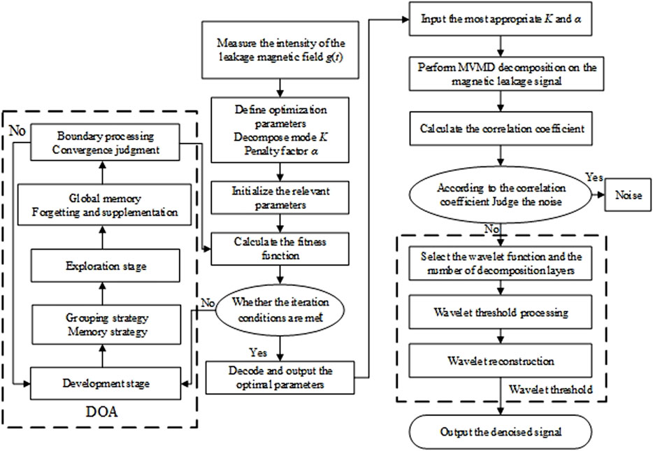
Figure 1. DOA optimizes MVMD parameters and combines wavelet threshold method.

3 Transformer fault diagnosis based on improved ELM

3.1 ELM algorithm

After denoising the measured leakage magnetic field signal by improving MVMD and combining with the wavelet threshold, the fault characteristic values of the signal are extracted, and the ELM algorithm is used for fault diagnosis. The ELM network adopts a single-hidden-layer feedforward neural network architecture. Its core feature lies in that the connection weights w_i from the network input layer to the hidden-layer and the bias parameters b_i of the hidden-layer nodes both adopt a random initialization strategy. Only the connection weights β_i from the hidden-layer nodes to the output layer need to be solved through matrix operations to complete the network training (Jian et al., 2025).

First is the training process. Suppose there is a labeled training sample set for early faults of transformers $\left(x_i,t_i\right)$, i = 1,2… N, where, $x_i={\left[x_{i1},x_{i2},\dots x_{in}\right]}^T\in R^n$ represents the sample characteristics; $t_i={\left[t_{i1},t_{i2},\dots t_{im}\right]}^T\in R^m$ Represent the label of sample i in Class m, $t_{ij}\in \left\{0,1\right\}$ j = 1,2… m, as shown in Formula 16, there are L hidden nodes (L ≤ N). The mathematical model is shown as follows:

$t_j={\displaystyle \sum _{i=1}^L}{\beta }_{i}g\left(w,b,x\right)={\displaystyle \sum _{i=1}^L}{\beta }_{i}h\left(x\right)(16)$

$g\left(w_i,b_i,x_i\right)$ represents the activation function of the ith node in the hidden layer and the way to connect to the output layer. Equation 16 can be simplified as follows Equation 17:

$H\beta =T(17)$

The output matrix of the hidden layer is as follows Equations 18, 19

$H={\left[\begin{array}{ccc}g\left(w_1,b_1,x_1\right)& \dots & g\left(w_L,b_L,x_1\right)\\ ⋮& \ddots & ⋮\\ g\left(w_1,b_1,x_N\right)& \dots & g\left(w_L,b_L,x_N\right)\end{array}\right]}_{N\times L}(18)$

$\beta ={\left[\begin{array}{l}{\beta }_1^T\\ ⋮\\ {\beta }_L^T\end{array}\right]}_{L\times m}T={\left[\begin{array}{l}{t}_1^T\\ ⋮\\ t_N^T\end{array}\right]}_{N\times m}(19)$

The parameters of Equation 17 can be converted into least squares solutions for calculation using Equation 20:

$\min ‖H\beta -T‖(20)$

The least squares solution obtained through calculation is:

$\beta =H^{+}T={\left(H^{T}H\right)}^{-1}{H}^{T}T(21)$

In the Equation 21: $H^{+}$ represents the M-P generalized inverse of the H matrix.

After the model training is completed, the output weight matrix β obtained through learning is used to predict the test set data to obtain the output result of the network. By comparing whether the index position corresponding to the maximum value in the output matrix matches the position of the true label of the sample, it can be determined whether the fault type identification of the test sample is correct.

3.2 ELM algorithm based on DOA optimization

Compared with the BP neural network, although the ELM has significant advantages in terms of training speed, generalization performance and global optimization ability, the input weights w_i and bias b_i of its hidden layer nodes adopt a random initialization strategy, resulting in the lack of tunability of neuron parameters. To this end, in this study, the DOA is introduced to optimize the key parameters of ELM, and the DOA-ELM hybrid model is constructed to improve the classification accuracy and robustness of the algorithm. Its process framework is shown in Figure 2. Firstly, feature extraction is carried out on the denoised magnetic leakage signal. Then, the sample data is divided into the training set and the test set and normalized preprocessing is conducted. Finally, the optimized DOA-ELM model is adopted to complete the fault classification task.

Figure 2

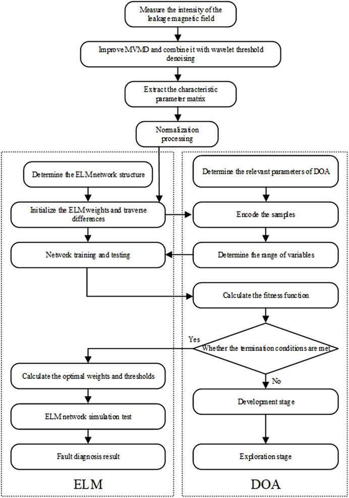
Figure 2. Transformer fault diagnosis flowchart based on DOA-ELM.

4 Analysis of leakage magnetic field characteristics in transformer winding faults

4.1 Simulation model construction

Based on the specific parameters of a certain actual three-phase three-column transformer, the corresponding finite element analysis model was constructed in this paper on the ANSYS Electronics Desktop simulation platform. This model is mainly used to study the influence of initial faults such as winding deformation and inter-turn short circuit on the electrical characteristics of transformers. The specific structural parameters and electrical parameters of the model are listed in Tables 1, 2 respectively.

Table 1

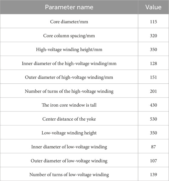
Table 1. Transformer structure parameters.

Table 2

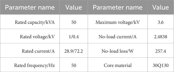
Table 2. Transformer electrical parameters.

When establishing the transformer simulation model, considering the complexity of the actual structure, this study adopts a reasonable simplification processing method. Based on the assumption of structural symmetry, the model mainly consists of key components such as the core, windings and yoke. Among them, the high and low voltage windings are idealized: It is assumed that the wires are uniformly and closely arranged, the current distribution remains uniform, and the block modeling method is adopted. Meanwhile, to simplify the calculation, the interference effects of secondary factors such as the interlayer structure of the winding, the oil tank and the supporting components on the leakage magnetic field are temporarily not considered in the model.

When the transformer windings undergo deformation or inter-turn short circuit faults, the spatial distribution characteristics of the leakage magnetic field will change significantly. Considering this characteristic, in this paper, the leakage magnetic field parameter is selected as the characteristic index characterizing the early fault state of the winding. During the finite element modeling process, A monitoring path was set around the A-phase winding on the high-voltage side to capture the dynamic changes of the leakage magnetic field during the fault development process. Considering that the installation position of the optical fiber magnetic field sensor in the actual experiment is fixed and cannot be adjusted, finally, five virtual measurement points at fixed positions were set along this path in the simulation model to obtain the magnetic induction intensity data at key positions. The three-dimensional finite element model of the transformer is shown in Figure 3. The measurement path of the transformer and the installation position of the virtual measurement points are shown in Figure 3.

Figure 3

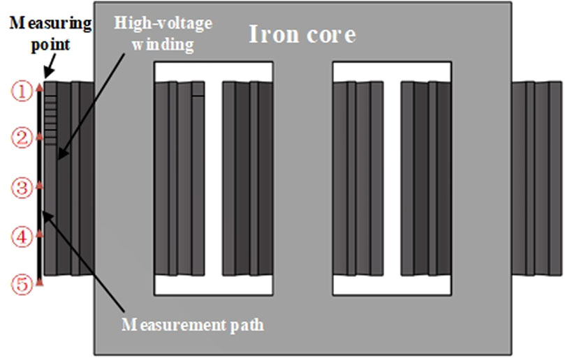
Figure 3. Transformer measurement path and virtual measurement point distribution.

4.2 Analysis of leakage magnetic field distribution characteristics in early faults of transformer windings

The finite element method is adopted to numerically solve the magnetic field distribution of the transformer. By introducing the magnetic vector position A as the calculation variable and using the iterative algorithm to discretize the solution area, the numerical solutions of the magnetic vector positions of each discrete node are finally obtained (Xiangli et al., 2023b).

$B=\nabla \times A(22)$

In the Equation 22: B respects magnetic induction intensity; A is the magnetic vector potential; ▽ is the curl operator.

From the formula, it can be solved that the corresponding B value at the corresponding position within the solution region is:

$B=\sqrt{{\left(\frac{\mathit{\partial }A}{\mathit{\partial }x}\right)}^2+{\left(\frac{\mathit{\partial }A}{\mathit{\partial }y}\right)}^2}(23)$

In the Equation 23 x: axial direction, i.e., taking partial derivative with respect to the axial direction; y: radial direction, i.e., taking partial derivative with respect to the radial direction.

4.2.1 Single-ended axial compression of the high-voltage side winding

The analysis of the mechanical characteristics of the transformer winding under the action of electromagnetic force shows that the radial magnetic field will cause an axial compressive force at the end of the winding, making it show an axial contraction trend. The axial magnetic field, on the other hand, generates radial expansion force, causing the winding to expand outward. Under actual operating conditions, when a short-circuit fault occurs, the huge short-circuit electromotive force will destroy the dynamic stability of the winding, resulting in permanent deformation. Given the complexity of the operating environment and the diversity of deformation modes, this paper only discusses the common single-mode winding deformation faults of transformers.

Taking the axial compression deformation of the A-phase high-voltage winding as an example, with deformation degree of 10%, the distribution of the transformer leakage magnetic field along different measurement paths in the axial and radial directions is shown in Figures 4, 5, under the condition of single-ended axial compression.

Figure 4

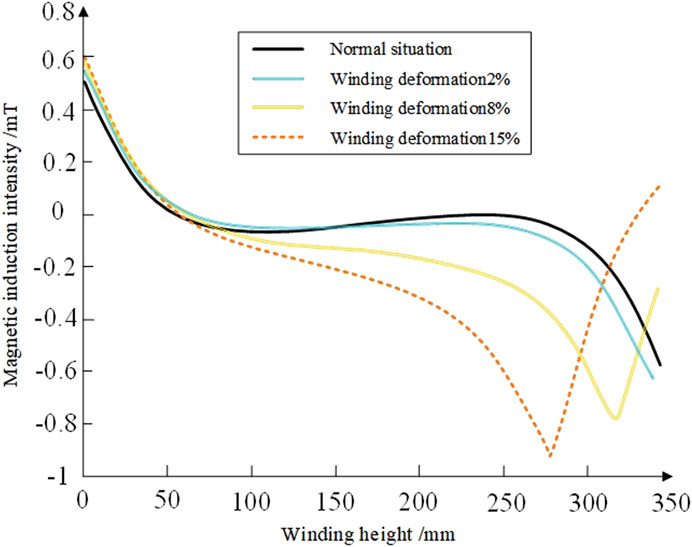
Figure 4. Radial magnetic induction intensity.

Figure 5

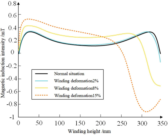
Figure 5. Axial magnetic induction intensity.

It can be known from Figure 4 that when the transformer winding is in a normal condition, that is, without deformation, the axial leakage magnetic field and the radial leakage magnetic field are symmetrical. Moreover, the axial magnetic induction intensity is the smallest at the first and last ends, reaches the maximum value in the middle of the winding, and the amplitude variation trend is obvious at the end of the winding. The radial magnetic induction intensity reaches its maximum value at the beginning and end of the winding and is in opposite directions. When it reaches the middle of the winding, it is nearly zero. Therefore, under normal circumstances, the leakage magnetic field intensity is mainly determined by the axial leakage magnetic field. When the winding undergoes single-ended axial compression, the symmetry of the leakage magnetic field distribution on the measurement path is disrupted. With the increase of the deformation degree, the distortion degree of the leakage magnetic field is also getting larger and larger. For the radial magnetic induction intensity, most of the radial magnetic induction intensity along the measurement path has changed. Only the area far from the deformation part has little change. The place with the greatest change in radial magnetic induction intensity occurs at the point where the deformation occurs. For the axial magnetic induction intensity, the axial magnetic induction intensity along the measurement path has all changed. The place where the axial magnetic induction intensity changes the most occurs is near the place where the deformation occurs.

4.2.2 Inter-turn short circuit of the high-voltage side winding

During the operation of the transformer winding, the inter-turn insulation may deteriorate due to insufficient short-circuit resistance, which in turn leads to inter-turn short-circuit faults. To study the influence of A slight inter-turn short circuit on the leakage magnetic field, a simplified simulation model is established in this paper: It is assumed that only the A-phase winding on the high-voltage side has a single-turn short circuit, while the other two phases maintain normal operation. The on-off state of the short-circuit circuit is controlled by applying pulse voltage signals with specific parameters, thereby simulating the inter-turn short-circuit condition.

The simulation results show that when inter-turn short circuits occur at different positions in the A-phase winding at 40 m, short-circuit currents dozens of times the rated value will be generated in the faulty turns, and significant leakage magnetic field distortion will be caused. Figures 6, 7 show the distribution of the leakage magnetic field corresponding to the moment when the short-circuit current reaches its peak, and obvious abnormalities in the magnetic field distribution can be observed.

Figure 6

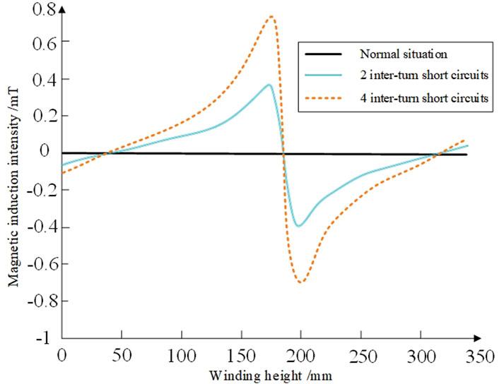
Figure 6. Radial magnetic induction intensity distribution of inter-turn short circuit.

Figure 7

Figure 7. Axial compression magnetic induction intensity distribution of single end.

When an inter-turn short circuit fault occurs in the transformer winding, its leakage magnetic field characteristics will change significantly, as shown in Figures 6, 7. Moreover, both the radial and axial magnetic induction intensities will show significant enhancement. This enhancement effect can be detected not only near the short-circuit point but also in the more distant areas. Furthermore, the degree of magnetic field distortion shows an obvious gradient feature, that is, the closer to the short-circuit point, the more significant the increase in magnetic field intensity. This phenomenon occurs because a low-impedance circuit is formed between the short-circuit turn and the normal winding, and the intensity of the circulating current generated in this circuit can reach dozens of times the normal operating current (Richang et al., 2021). As the degree of the fault intensifies, the circulating current effect will be further amplified, thereby causing the distortion degree.

4.3 Fault feature extraction

The above analysis indicates that when early faults occur in transformer windings, the distribution of leakage magnetic field will exhibit regular changes in spatial symmetry, waveform shape, amplitude differences, and positional correlation, which can accurately reflect the operating status of the windings. To comprehensively capture these features for accurate diagnosis, this study selected the leakage magnetic induction intensity at different positions of the upper, middle, and lower parts of the winding as the key feature parameter measurement points. The distribution difference, correlation coefficient, Hausdorff distance, and asymmetry can evaluate the different characteristics between waveforms. Therefore, monitoring the spatial distribution characteristics of the leakage magnetic field inside the transformer and evaluating the above indicators can effectively diagnose early faults in the winding.

Suppose there are two leakage magnetic field curves, $B_0=\left\{b_{01},b_{02},...,b_{0n}\right\}$, $B=\left\{b_1,b_2,...,b_n\right\}$, B₀ represents the magnetic induction intensity of the leakage magnetic field under normal conditions, B represents the magnetic induction intensity data of the leakage magnetic field during faults, and n represents the number of data points.

4.3.1 Distribution difference degree

By comparing and analyzing the magnetic field data of each measurement point, it was found that when the fault occurred in the upper area of the winding, the cumulative deviation values of the magnetic induction intensities collected at measurement points 4 and 5 from the normal state were significantly higher than those at measurement points 1 and 2. Conversely, when the fault is located at the lower part of the winding, the opposite distribution characteristics are presented. This regular change can be used as the basis for determining the asymmetric fault location of the winding, and its quantitative expression is as follows Equation 24:

$\left\{\begin{array}{l}{H}_1={\displaystyle \sum _n}\left|\Delta B\left(x_1\right)\right|-{\displaystyle \sum _n}\left|\Delta B\left(x_5\right)\right|\\ H_2={\displaystyle \sum _n}\left|\Delta B\left(x_2\right)\right|-{\displaystyle \sum _n}\left|\Delta B\left(x_4\right)\right|\end{array}\right.(24)$

In the formula: $\sum \left|\Delta B\left(x_i\right)\right|$ represents the sum of the absolute deviations of the fault data and the normal data at the ith measurement point at n sampling points. Based on the difference in magnetic field distribution between normal working conditions and symmetrical faults, a characteristic threshold interval is set for fault location: when the characteristic value exceeds the upper limit of the threshold, it is marked as 1, that is, the lower fault; When it is lower than the lower limit, it is marked as 0, that is, the upper part is faulty. If it is within the threshold range, it is marked as 0.05, that is, the middle fault. Furthermore, for the asymmetric winding structure, the asymmetry degree parameter and the distribution difference degree parameter need to be initialized to zero values for processing. This quantification method achieves the precise location of the winding fault area by establishing the mapping relationship between the eigenvalues and the fault location.

4.3.2 Correlation coefficient

The correlation coefficient (CC), as an effective waveform similarity measurement index, can accurately represent the morphological difference characteristics of the two curves. When analyzing asymmetric faults, the fault measurement points will not only show amplitude changes, but also produce obvious phase offset phenomena. This dual variation characteristic makes the correlation coefficient particularly suitable for identifying asymmetric faults with slight deformation. Its calculation formula is as follows Equation 25:

$C=\frac{{\displaystyle {\sum }_{i=1}^n}{B}_i{B}_{0i}}{\sqrt{{\displaystyle {\sum }_{i=1}^n}{\left[B_{0i}\right]}^2{\displaystyle {\sum }_{i=1}^n}{\left[B_i\right]}^2}}(25)$

Under the normal operating conditions of the transformer, the correlation coefficients of the two leakage magnetic field curves usually approach 1, indicating that their waveforms have a high degree of similarity. When faults such as winding deformation or inter-turn short circuit occur, the CC values at each measurement point will decrease to varying degrees. In particular, when the fault causes significant distortion of the waveform, the CC value may drop to the order of 0.01–0.001, reflecting severe waveform differences. Among them, n represents the number of sampling points and is an important parameter for calculating the correlation coefficient.

4.3.3 Hausdorff distance

The Hausdorff distance, as an effective curve similarity measurement index, can simultaneously reflect the comprehensive differences in waveform shape and amplitude size. Research shows that when a transformer malfunctions, the Hausdorff distance between the measured leakage magnetic field curve and the reference curve monotonically increases with the intensification of the fault degree. Its mathematical expression is as follows Equation 26:

$\left\{\begin{array}{l}H\left(B_0,B\right)=\max \left\{h\left(B_0,B\right),h\left(B,B_0\right)\right\}\\ h\left(B_0,B\right)=\underset{B_{0i}\in B_0}{\max }\left\{\underset{B_j\in B}{\min }‖B_{0i},B_j‖\right\}\\ h\left(B,B_0\right)=\underset{B_j\in B}{\max }\left\{\underset{B_{0i}\in B_0}{\min }‖B_{0i},B_j‖\right\}\end{array}\right.(26)$

4.3.4 Asymmetry

Under the normal operating state of the transformer, the spatial distribution of the leakage magnetic field shows obvious symmetrical characteristics. However, when asymmetric faults occur in the windings, this symmetrical distribution feature will change significantly, and the more severe the fault is, the more obvious the symmetry disruption of the magnetic field distribution will be. Based on this physical phenomenon, the asymmetry index is used to quantify the fault characteristics, and its mathematical expression is as follows Equation 27:

$\left\{\begin{array}{l}{\eta }_1=\frac{{\displaystyle {\sum }_n}\left|B\left(x_1\right)-B\left(x_5\right)\right|}{{\displaystyle {\sum }_n}\left|B\left(x_1\right)+B\left(x_5\right)\right|}\\ {\eta }_2=\frac{{\displaystyle {\sum }_n}\left|B\left(x_2\right)-B\left(x_4\right)\right|}{{\displaystyle {\sum }_n}\left|B\left(x_2\right)+B\left(x_4\right)\right|}\end{array}\right.(27)$

In the formula, B(x_i) represents the leakage magnetic field distribution data obtained from the ith monitoring point. When the transformer is operating normally, the asymmetry index remains at a relatively low level. When asymmetric faults occur, the value of this parameter will increase significantly. Although the asymmetry index cannot precisely locate the specific position where the fault occurs, as an auxiliary diagnostic parameter, it can effectively determine whether there is an asymmetry fault phenomenon in the winding.

5 Simulation and dynamic model experiment verification

5.1 Simulation verification of early fault diagnosis of transformers

After the noisy leakage magnetic field signal undergoes the above noise reduction processing, four characteristic values, namely, the correlation coefficient, asymmetry degree, distribution difference degree and Hausdorff distance, are extracted. Then, the DOA-ELM algorithm is used to realize the fault mode recognition.

In the section on building the simulation model in 4.1, it is mentioned that the main research focuses on two types of faults: winding deformation and inter-turn short circuit. Depending on the location of the fault in the winding, there are specifically six scenarios. This paper considers six common faults of transformer windings, including inter-turn short circuit in the upper part of the winding, inter-turn short circuit in the middle part of the winding, inter-turn short circuit in the lower part of the winding, compression deformation at the beginning of the winding, compression deformation at the end of the winding, and compression deformation at both ends of the winding. Magnetic field data of five monitoring points are collected under each fault condition. After feature extraction, a feature vector including the correlation coefficient, asymmetry degree, distribution difference degree and Hausdorff distance is formed. A total of 300 sample datasets were constructed for the simulation, including 150 sets of data each for inter-turn short circuit faults and winding deformation faults. After dividing these samples into the training set and the test set, normalization processing was carried out respectively. To ensure the training effect and improve the generalization ability of the model, hierarchical random sampling was adopted to construct the training set, including 240 groups of training data and 60 groups of test data, and standardized preprocessing was performed on all feature data.

Take the 240 groups of extracted training samples as one dataset, where i = 1,2… 240, bring it into the DOA-ELM classifier for training. Among them, the number of input layer nodes of the DOA-ELM network is 240; The number of nodes in the output layer is the same as the dimension of the sample labels. Set the number of nodes i in the hidden layer to 45 and the hidden layer activation function to “sigmoid”. Utilize the obtained output weight matrix to conduct testing on the test dataset, and perform comparative analysis between the DOA-ELM classification method and the BPNN, SVM, and CNN classification methods.

The number of hidden layer nodes in BPNN is an important factor affecting the classification performance. In order to compare the effects of DOA-ELM and BPNN, the number of hidden layer nodes is also set to 45, and then the training error is set to 1 × 10⁻⁶. With “newff” as the network creation function and “train” as the training function, “sim” is used as the test function. The kernel function of SVM is the radial basis. Among them, the penalty factor is 10 and the kernel parameter is 0.5. The CNN model adopts an architecture consisting of 3 convolutional layers (with kernel sizes of 3 × 3, 5 × 5, and 3 × 3 respectively) + 2 pooling layers (max pooling, with a stride of 2 × 2) + 1 fully connected layer. The learning rate is set to 0.001, and the number of iterations is 50 rounds.

The classification results of the DOA-ELM method are shown in Figures 8, 9. The operation results and comparisons of various methods are shown in Table 3.

Figure 8

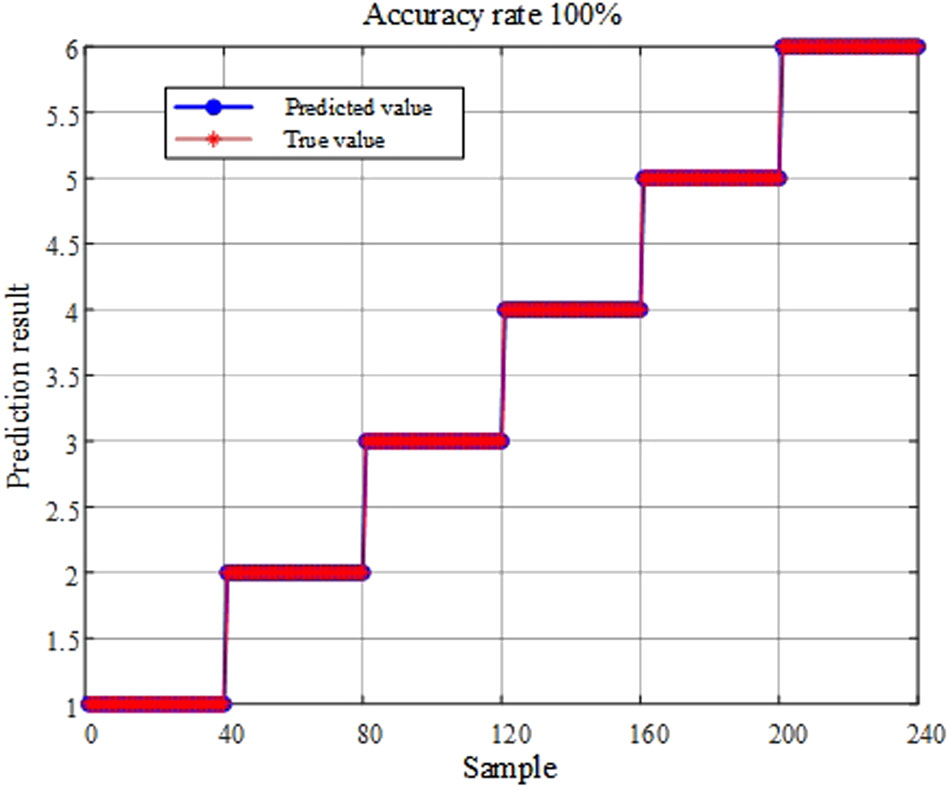
Figure 8. Accuracy rate of the training set.

Figure 9

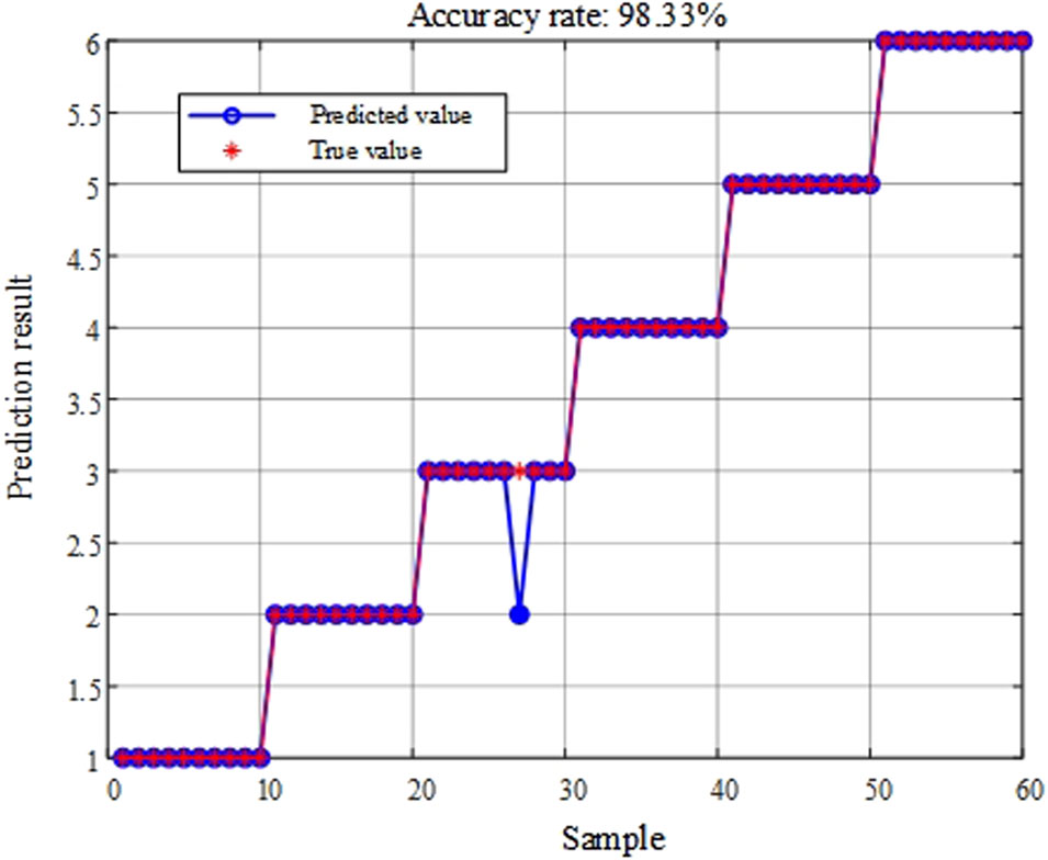
Figure 9. Accuracy rate of the test set.

Table 3

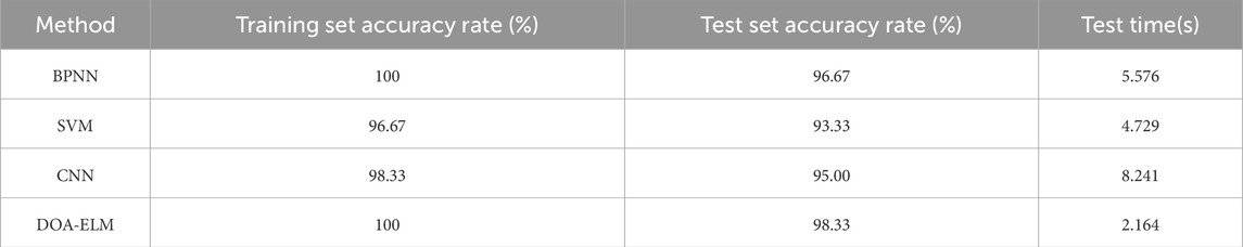
Table 3. Performance comparison of different classification methods.

As shown in Table 3, for the task of early fault classification of transformers, the DOA-ELM method proposed in this paper has the highest accuracy rate compared with BPNN and SVM, reaching the highest accuracy rate of 98.33%. In terms of computational efficiency, the testing time of BPNN, SVM, and CNN is longer than that of DOA-ELM, making them unsuitable for rapid classification. This indicates that the method proposed in this paper not only exhibits excellent generalization performance, but also utilizes feature quantities capable of characterizing the state features of early transformer faults.

5.2 Dynamic mold test verification

To test the reliability of the fault diagnosis method in this paper, fault verification is carried out through relevant experiments. The primary wiring diagram is shown in Figure 10. The three-phase transformer as shown in Figure 11 is adopted as the test object, and the optical fiber magnetic induction detection device as shown in Figure 12 is configured. The experimental parameters are detailed in Table 4.

Figure 10

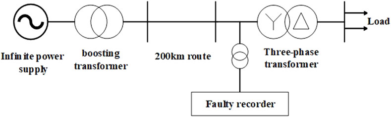
Figure 10. Dynamic mode transformer experimental primary wiring diagram.

Figure 11

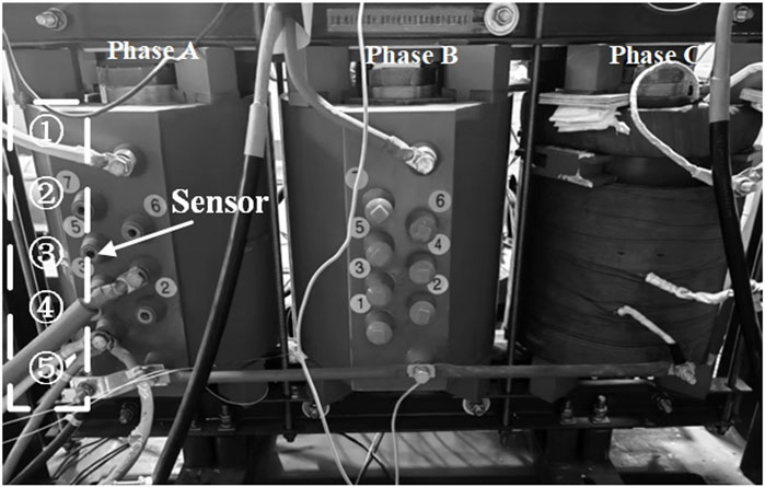
Figure 11. Experimental transformer.

Figure 12

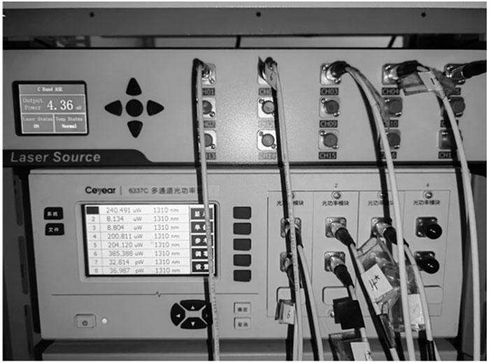
Figure 12. Optical fiber measurement system.

Table 4

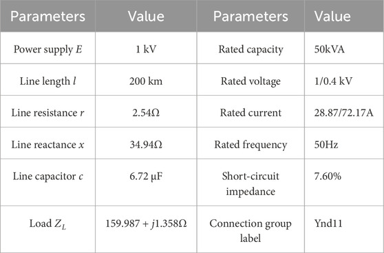
Table 4. Relevant parameters of dynamic simulation experiment system and transformer.

The experimental system is set up with a simulated voltage of 1 kV. The ideal power supply is simulated using a 50kVA transformer, and the 200 kM line is simulated using a π-type equivalent circuit. The test transformer is a specially made three-phase dry-type step-down transformer with a transformation ratio of 1/0.4 kV and a Y/△ wiring method. The neutral point of the transformer’s Y-side winding and the system neutral line are connected to the laboratory’s dedicated grounding grid through cables.

Turn-to-turn short circuit fault simulation: The winding to be tested for short circuit is connected to the short circuit controller through the tap terminal of the transformer winding, completing the turn-to-turn short circuit simulation experiment.

Winding deformation simulation: Through a precision mechanical device, axial pressure is applied to the winding ends to simulate the deformation caused by short-circuit electrodynamic forces. Spiral-type pressure mechanisms (including a stepper motor with a minimum adjustment of 0.01 mm) are installed at the top and bottom of the transformer’s high-voltage winding, accompanied by a laser displacement sensor (with an accuracy of 0.001 mm) to monitor the compression in real time, achieving varying degrees of winding deformation.

The dynamic simulation experiment not only realizes the physical process of early faults in transformer windings, but also ensures the reliability and repeatability of data through standardized operations. It also provides support for the transformation of this testing method from the laboratory to engineering applications.

5.2.1 Noise reduction of measured transformer leakage magnetic field signal

In order to verify the feasibility of the improved MVMD algorithm in practical applications, this paper takes the measured data of Sensor No. 1 and Sensor No. 2 of the transformer winding under the normal operating state as an example, and adopts the improved MVMD method to carry out noise reduction processing on them. Figure 13 shows the comparison between the original magnetic leakage signal and the signal after noise reduction using the method proposed in this paper. Figure 14 respectively show the modal diagrams after the decomposition of MVMD and their corresponding spectral diagrams.

Figure 13

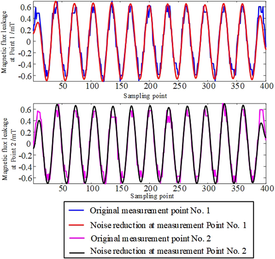
Figure 13. Comparison of denoising methods in this paper.

Figure 14

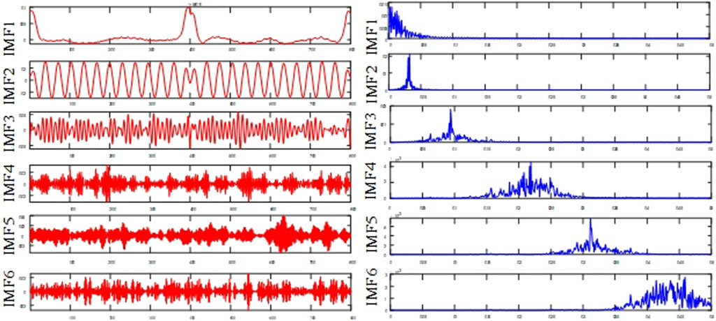
Figure 14. Modes and spectrograms after MVMD decomposition.

To further verify the superiority of the denoising method proposed in this paper, Table 5 compares the performance indicators of different denoising methods, including signal-to-noise ratio, mean square error and cross-correlation number.

Table 5

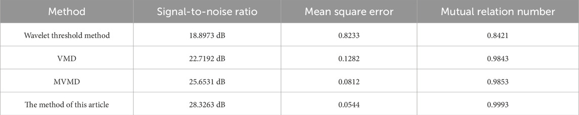
Table 5. Comparison of denoising methods.

It can be known from Table 5 that the signal-to-noise ratio of the traditional wavelet threshold method is relatively low, indicating that it has certain limitations when processing complex signals. In contrast, both the VMD and MVMD methods have significant improvements in signal-to-noise ratio, mean square error, and the number of cross-correlations, demonstrating better denoising effects. However, the method proposed in this paper is superior to VMD and MVMD in terms of signal-to-noise ratio, mean square error and cross-correlation number, indicating that it has significant advantages in suppressing noise interference, improving signal quality and maintaining the integrity of signal characteristics. This provides more reliable data support for the subsequent fault diagnosis of transformers.

5.2.2 Dynamic model verification of fault diagnosis model

After noise reduction processing of the collected magnetic field signals, the DOA-ELM algorithm was used to conduct fault diagnosis on the 90 groups of samples obtained from the experiment. Among the data of the 90 groups of samples, there were 60 groups of inter-turn short circuit faults and 30 groups of winding deformation faults. The classification results are shown in Figure 15. The experimental data indicate that the diagnostic model proposed in this paper can effectively distinguish different types of transformer faults and has a high recognition accuracy rate.

Figure 15

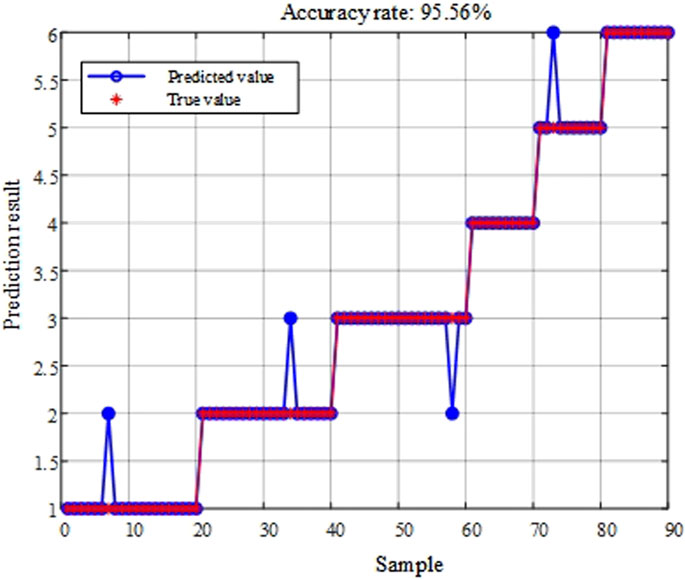
Figure 15. Dynamic mold verification.

5.3 Distribution of fault sample categories and analysis of data balance

5.3.1 Sample category distribution table

The classification distribution of simulation experiment samples and the classification distribution of dynamic simulation experiment samples are shown in Tables 6, 7.

Table 6

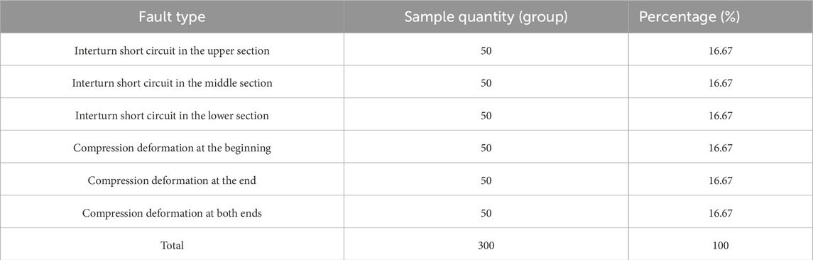
Table 6. Distribution of sample categories in simulation experiments.

Table 7

Table 7. Distribution of sample categories in dynamic simulation experiments.

5.3.2 Analysis of the impact of data imbalance on model performance

In the simulation experiment, the sample size of 6 types of faults was evenly distributed (all 50 groups), accounting for 16.67% of the total. This balanced distribution can avoid the model being biased towards the majority class due to differences in sample size, ensuring that each fault feature is fully learned during the training process. The experimental results show that the DOA-ELM model has a recognition accuracy of over 96% for all types of faults (with an average accuracy of 98.0% for inter turn short circuit faults and 97.5% for deformation faults), verifying the stability performance of the model under balanced data.

In the dynamic simulation experiment, there were 20 groups of inter turn short circuit faults (upper, middle, and lower sections) each (accounting for 22.22%), while there were 10 groups of deformation faults (head, end, and two ends) each (accounting for 11.11%), indicating a certain degree of imbalance (quantity ratio 2:1). The results showed that the accuracy of deformation type faults with a small sample size was slightly lower (a difference of 3.34%), but the overall accuracy remained at 95.56%. This indicates that the DOA-ELM model has strong generalization ability through DOA optimized parameters, and still has good recognition performance for small sample categories. The impact of data imbalance is within an acceptable range.

The balanced data from the simulation experiment validated the stable identification ability of the model for various types of faults; The slight imbalance in the dynamic simulation experiment resulted in a slight decrease in the accuracy of a few classes, but did not significantly affect the overall performance. Therefore, the proposed method has a certain adaptability to data distribution, and even with slight imbalances, it can still meet engineering requirements.

The balanced distribution data from the simulation experiment validated the stable identification ability of the model for various types of faults; The slight imbalance distribution data in the dynamic simulation experiment resulted in a slight decrease in the accuracy of a few classes, but did not significantly affect the overall performance. Therefore, the proposed method has a certain adaptability to data distribution, and even with slight imbalances, it can still meet engineering requirements.

6 Conclusion

This paper proposes an early fault diagnosis method for transformer windings based on improved MVMD denoising and optimized ELM. Firstly, a finite element model of the transformer was established using ANSYS. The distribution characteristics of the leakage magnetic field under fault conditions such as axial compression deformation of the winding and inter-turn short circuit were simulated and analyzed. Multi-dimensional fault features such as the correlation coefficient, asymmetry degree, distribution difference degree and Hausdorff distance were extracted as the diagnostic basis. Secondly, the correlation decomposition mode number K and penalty factor α of MVMD are adaptively adjusted through the DOA, and the secondary noise reduction processing of the noisy magnetic leakage signal is carried out in combination with the wavelet threshold method, which improves the signal-to-noise ratio and feature retention ability of the signal. Finally, an ELM fault diagnosis model based on DOA optimization was constructed. By adaptively adjusting the input weights and bias parameters of the network, the classification performance of the model was improved. Verified through simulation and dynamic model experiments, the results show that the proposed method has excellent performance in the early fault diagnosis of transformer windings. The accuracy rate of the simulation experiment reaches 98.33%, and the accuracy rate of the dynamic model experiment reaches 95.56%, which is superior to the traditional BPNN and SVM methods. This method has obvious advantages in signal processing and fault classification, providing an effective technical means for the precise diagnosis of early faults in transformer windings and having certain working value.

Data availability statement

The original contributions presented in the study are included in the article/supplementary material, further inquiries can be directed to the corresponding author.

Author contributions

QL: Writing – original draft, Conceptualization, Writing – review and editing, Data curation, Methodology. CW: Formal Analysis, Data curation, Writing – original draft, Investigation. LZ: Writing – original draft, Software, Investigation. FZ: Formal Analysis, Supervision, Writing – review and editing. ZZ: Supervision, Writing – original draft, Methodology. MW: Project administration, Writing – original draft. JL: Conceptualization, Writing – original draft, Supervision. CL: Methodology, Formal Analysis, Writing – review and editing.

Funding

The author(s) declare that no financial support was received for the research and/or publication of this article.

Conflict of interest

Authors QL, CW, LZ, FZ, ZZ, MW, JL, and CL were employed by Sanmen Nuclear Power Co., Ltd.

Generative AI statement

The author(s) declare that no Generative AI was used in the creation of this manuscript.

Any alternative text (alt text) provided alongside figures in this article has been generated by Frontiers with the support of artificial intelligence and reasonable efforts have been made to ensure accuracy, including review by the authors wherever possible. If you identify any issues, please contact us.

Publisher’s note

All claims expressed in this article are solely those of the authors and do not necessarily represent those of their affiliated organizations, or those of the publisher, the editors and the reviewers. Any product that may be evaluated in this article, or claim that may be made by its manufacturer, is not guaranteed or endorsed by the publisher.

References

Athikessavan, T. C., Jeyasankar, E., Manohar, S. S., and Panda, S. K. (2019). Inter-turn fault detection of dry-type transformers using core-leakage fluxes. IEEE Trans. Power Deliv. 34 (4), 1230–1241. doi:10.1109/tpwrd.2018.2878460

CrossRef Full Text | Google Scholar

Chao, P., Wenxin, S., and Tao, M. (2020). Study on electromagnetic characteristics of interturn short circuit ofSingle-phase transformer. High. Volt. Eng. 46 (05), 1839–1856.

Google Scholar

Dragomiretskiy, K., and Zosso, D. (2014). Variational mode decomposition. IEEE Trans. Signal Process. 62 (3), 531–544. doi:10.1109/tsp.2013.2288675

CrossRef Full Text | Google Scholar

Hongda, L. I., Dingkun, H., Bin, Z., et al. (2020). Research in detection of winding transformer variationbased on improved LVI method. J. Nanjing Univ. Sci. Technol. 44 (01), 15–20. doi:10.14177/j.cnki.32-1397n.2020.44.01.003

CrossRef Full Text | Google Scholar

Jian, Z., Beiping, X., Lei, N. I., et al. (2018). Research on adaptive wavelet packet threshold function denoising algorithm based on Shannon entropy. J. Vib. Shock 37 (16), 206–211.

Google Scholar

Jian, Z., Mi, Z., Yi, H., et al. (2025). Research on fault diagnosis method of pv array based on cld-coa-elm. Acta Energiae Solaris Sin. 46 (01), 632–640. doi:10.19912/j.0254-0096.tynxb.2023-1468

CrossRef Full Text | Google Scholar

Jianfeng, L., Mengqi, L., Qianwen, D., et al. (2023). Transformer early fault diagnosis based on improved VMD denoising andoptimized ELM method. J. Electr. Power Sci. Technol. 28 (06), 55–66. doi:10.19912/j.0254-0096.tynxb.2022-1986

CrossRef Full Text | Google Scholar

Jianfeng, L., Zhiyuan, L. I., and Yaru, Z. (2024). Transformer windings based on leakage field and ICOA-ResNet early fault diagnosis. Power Syst. Prot. Control 52 (09), 99–110. doi:10.19783/j.cnki.pspc.231278

CrossRef Full Text | Google Scholar

Jiang, C., Junxiang, T., Zhuoran, Z., et al. (2018). Fast fault classification method research of aircraft generator rotating rectifier based on extreme learning machine. Proc. CSEE 38 (8), 2458–2466. doi:10.16081/j.epae.201912021

CrossRef Full Text | Google Scholar

Lang, Y., and Gao, Y. (2025). Dream Optimization Algorithm (DOA): a novel metaheuristic optimization algorithm inspired by human dreams and its applications to real-world engineering problems. Comput. Methods Appl. Mech. Eng. 436, 117718. doi:10.1016/j.cma.2024.117718

CrossRef Full Text | Google Scholar

Mao, J. I., Bo, Q. I., Wei, Z., et al. (2024). Coding diagnosis method based on leakage distribution law under typical winding defects of transformers. Power Syst. Technol. 48 (05), 2133–2142. doi:10.13335/j.1000-3673.pst.2023.1694

CrossRef Full Text | Google Scholar

Rehman, N. U., and Aftab, H. (2019). Multivariate variational mode decomposition. IEEE Trans. Signal Process. 67 (99), 6039–6052. doi:10.1109/TSP.2019.2951223

CrossRef Full Text | Google Scholar

Richang, X., Bingqian, Z., Xinghua, L., et al. (2021). Application of finite element analysis to transient characteristics of interturn short circuit in power transformer windings. Electr. Mach. Control 25 (10), 130–138. doi:10.15938/j.emc.2021.10.014

CrossRef Full Text | Google Scholar

Tao, F., Ye, Q., Canjie, G., et al. (2020). Research on transformer fault diagnosis based on a beetle antennae search optimized support vector machine. Power Syst. Prot. Control 48 (20), 90–96. doi:10.19783/j.cnki.pspc.191534

CrossRef Full Text | Google Scholar

Wei, G., Shengbo, S., Peng, T., et al. (2024). Short-term photovoltaic power forecasting based on multivariate variational mode decomposition and hybrid deep neural network. Acta Energiae Solaris Sin. 45 (04), 489–499. doi:10.19912/j.0254-0096.tynxb.2022-1986

CrossRef Full Text | Google Scholar

Wenqing, Z., Hai, Y., Zhendong, Z., et al. (2020). Fault diagnosis of transformer based on residual BP neural network. Electr. Power Autom. Equip. 40 (2), 143–148. doi:10.16081/j.epae.201912021

CrossRef Full Text | Google Scholar

Xiangli, D., Yuelin, L., Hongye, Z., et al. (2023a). Early fault identification for a transformer based on current dynamic time warping difference of a digital twin model. Power Syst. Prot. Control 51 (12), 156–167. doi:10.19783/j.cnki.pspc.221634

CrossRef Full Text | Google Scholar

Xiangli, D., Kang, Y., Hongye, Z., et al. (2023b). Transformer winding early fault protection based on circuit-magnetic leakage field multi-state analytical model. Power Syst. Technol. 47 (09), 3808–3821. doi:10.13335/j.1000-3673.pst.2022.2015

CrossRef Full Text | Google Scholar

Xiangli, D., Qian, M. A., Zhixiang, T., et al. (2024a). Research on transformer incipient fault protection based on virtual leakage FieldWaveform of the digital twin model. Power Syst. Technol. 48 (11), 4806–4815. doi:10.13335/j.1000-3673.pst.2023.2067

CrossRef Full Text | Google Scholar

Xiangli, D., Hongye, Z., Kang, Y., et al. (2024b). Research on magnetic balance protection of transformers based on optical fiber leakage magnetic field measurement. Trans. China Electrotech. Soc. 39 (03), 628–642. doi:10.19595/j.cnki.1000-6753.tces.221959

CrossRef Full Text | Google Scholar

Yan, W., Wei, L. I., Hongshan, Z., et al. (2023). Transformer DGA fault diagnosis method based on DBN-SSAELM. Power Syst. Prot. Control 51 (04), 32–42. doi:10.19783/j.cnki.pspc.220662

CrossRef Full Text | Google Scholar

Yuanchao, Z., and Xue, W. (2017). The online monitoring method of transformer winding deformation based onmagnetic field measurement. Electr. Meas. and Instrum. 54 (17), 58–63+87.

Google Scholar

Zhongyong, Z., Chao, T., Chengxiang, L., et al. (2019). Diagnosis method of transformer winding deformation faults based on frequency response Binary image. High. Volt. Eng. 45 (05), 15261534. doi:10.13336/j.1003-6520.hve.20181121010

CrossRef Full Text | Google Scholar