Abstract
This paper investigates the causal relationship between water pollution, industrial agglomeration, and economic growth in 11 Chinese provinces in China. Using a bootstrap autoregressive distributed lag (ARDL) analysis, we examine the estimated models’ stability and investigate the Granger causality relationships between system variables. The results indicate that our estimation provides evidence of a long-run relationship between water pollution, industrial agglomeration, and economic growth in China. The bidirectional running from other water pollution variables is confirmed from the casualty tests in Shanghai and Yunnan. Specifically, the unidirectional causality relationship running from industrial agglomeration and economic growth to water pollution provide statistical evidence of the important role that industrial agglomeration and economic growth play in increasing water pollution.
Introduction
After 40 years of reform and opening-up, China’s economy has an annual average gross domestic product (GDP) growth rate of more than 9%, which is far higher than the world economy’s average annual growth rate of less than 3%. However, with the rapid growth of China’s economy, the phenomenon of increasing environmental pollution has begun to appear along with it. Among the current series of ecological and environmental problems facing China, water pollution in river basins involves a wide area, affects large populations, and causes great harm (Mei and Feng 1993).
In China, the large and long Yangtze River covers 11 Chinese provinces, linking regional economic development in a vast area called the Yangtze River Economic Belt (YREB), as shown in Figure 1. The YREB contributes to over 40% of China’s economic growth. Thus, in September 2014, the State Council promulgated “The State Council guidance on the golden waterway to promote the development of the Yangtze River Economic Zone.” However, according to 2017 Report on the State of the Ecology and Environment in China, the Yangtze River basin and the 510 water quality sections monitored and classified as national standard IV ∼ V was 13.3% (the inferior class V accounted for 2.2%). Industrial wastewater and domestic wastewater discharge are currently the main sources of environmental water pollutants, and economic development is one of the leading factors impacting environmental water quality (Chen et al., 2019). Economic activities have heavily impacted the environmental and ecological conditions of the YREB. The Chinese government has focused on the economy and environment to create water conservation and sustainable utilization (Fang et al., 2006).
FIGURE 1
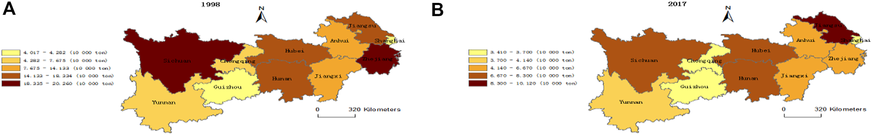
Water pollution of the YREZ. Light yellow represents the area with the least water pollution, as the color deepens, the degree of pollution becomes more serious, and dark red is the area with the most serious water pollution.
China attaches great importance to ecological and environmental issues and efforts to prevent environmental pollution. China has promoted ecological and environmental protection and reduced pollution emissions, but the ecological damage and environmental pollution caused by long-term, extensive economic development remains significant. According to data published in the “China Green National Accounting Study Report 2004,” the environmental degradation cost caused by water pollution was 286.28 billion yuan, accounting for 55.9% of the total environmental degradation cost, which was 1.71% of GDP in that year. Additionally, serious water pollution endangered the lives and health of residents. In 2004, the damage to the health of rural residents caused by water pollution amounted to 17.86 billion yuan. Figure 1 indicates the change in water pollution between 1998 and 2017. We found that water pollution in the Yangtze River’s upper and lower reaches saw large declines, but there was no significant change in its middle stretches.
This paper presents the impacts of industrial and economic factors on environmental water pollution in the YREB. GDP and industrial agglomeration play important roles in evaluating water pollution. Many studies believe that industrial agglomeration can increase productivity, thereby improving resource utilization efficiency and reducing pollutant emissions. Industrial agglomeration impacts environmental pollution in three ways: economies of scale, technology spillovers, and structural effects (Marshal 1920; Newman and Kenworthy 1989; Vukina et al., 1999). However, the increase in industrial agglomeration is the main reason for a series of ecological and environmental problems, such as water shortages, land occupation, soil degradation, air pollution, and a reduction in biodiversity in urban agglomerations (de Leeuw et al., 2001). As show in Figure 2, when the level of agglomeration is low, factor sharing among enterprises and intra-industry division of labor and complementarity have not yet formed, resulting in inefficient factor utilization and difficulty in realizing the knowledge spillover effect of clean technology (Ingstrup and Damgaard 2013). On the contrary, the rapid increase of resource consumption and pollutant discharge caused by inefficient agglomeration is likely to cause deterioration of environmental quality. With the improvement of the level of industrial agglomeration, a network of specialized division of labor and cooperation among enterprises that are interdependent and supportive is gradually formed, and knowledge spillover effects are generated through the exchange of technologies, thereby reducing the cost of technological innovation and motivating enterprises to increase R&D investment. Ultimately, the improvement of environmental quality will be promoted through the improvement of factor utilization efficiency and the innovation of clean technology.
FIGURE 2
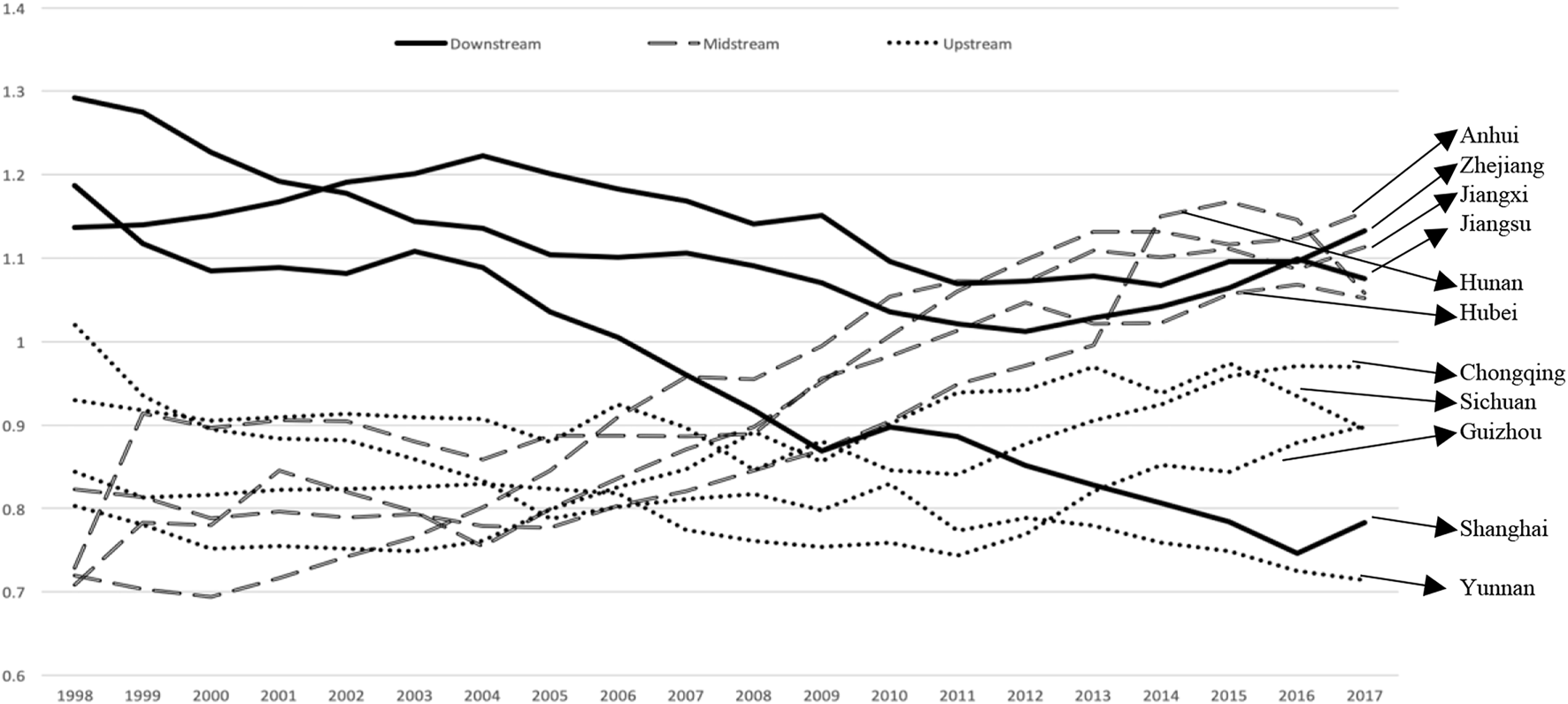
Industrial agglomeration of the YREZ.
The new economic geography theory holds that industrial agglomeration affects economic growth through three effects: economies of scale, knowledge spillovers and structural optimization. Marshall (2009) first proposed that the economies of scale of industrial agglomeration can reduce production and transaction costs and improve labor productivity (Glaeser et al., 1992) (Marshall 2009). However, according to the cluster life cycle theory, industrial agglomeration at a certain stage will also cause traditional industries to move out of the region, leading to the phenomenon of industrial diffusion, which in turn has a negative effect on economic growth (Glaeser et al., 1992).
The impact of environmental pollution on economic growth mainly depends on residents’ preference for environmental quality, which directly determines the impact of environmental pollution on economic growth. When the environmental quality-income elasticity is high, the negative effect of environmental pollution on economic growth is more significant. When the environmental quality-income elasticity is low, the effect of environmental pollution on economic growth will be restricted.
In the initial stage of economic growth, the reduction of production costs promotes the spatial agglomeration of labor-intensive industries. In the advanced stage of economic growth, the increase in R&D investment, the industrial transmission effect and the innovation environment effect absorb more high-tech industrial elements and promote the spatial agglomeration of high-tech industries.
There is also a feedback relationship between environmental pollution and industrial agglomeration. The “environmental production factor theory” believes that environmental pollution is actually the overuse of the environment as a production factor, and its impact on industrial agglomeration is positive and negative. When the cost of environmental factors is lower than other production factors, enterprises will use environmental factors to replace other factors such as technology and high-level labor. The low environmental cost further encourages enterprises to use funds to expand the scale of production. In this way, the pollution caused by environmental costs Dividends promote the formation of agglomeration of polluting enterprises in space (Tahvonen and Kuuluvainen 1993), that is, the impact of environmental pollution on industrial agglomeration is a positive effect. When the environmental cost is higher than other production factors, for example, the government raises the pollutant discharge tax of enterprises or raises the environmental protection standard, some polluting enterprises will migrate to the surrounding areas due to the increase of pollution cost and investment risk, and the health risks caused by pollution will also make Residents re-select their place of residence, which leads to the spread of production and population to the surrounding area, that is, environmental pollution has a negative effect (Lopez 2017).
The effect of industrial agglomeration on environmental pollution in the YREB needs to be tested. Industrial agglomeration in the middle reaches of the Yangtze River has greatly improved, and the industrial agglomeration in the downstream economically developed areas has shown a downward trend. This finding indicates that the Yangtze River industries have moved to inland China but have not yet moved to the river’s upper reaches because the industrial agglomeration in the upstream areas has not significantly improved.
The important contribution of this paper is that the three variables of economic growth, industrial agglomeration and water pollution are included in the same analysis framework, and the literature on the internal relationship between the three is relatively rare, and most of them use the panel econometric model and the traditional ARDL method. Panel data estimation cannot compare and discuss the differences between different provinces, and under the condition of non-stationary time series, using the classical regression equation to estimate the model will lead to the phenomenon of “pseudo-regression” (Coondoo and Dinda 2002). Although the traditional ARDL test can avoid serial correlation or random trend in time series, it is not suitable for small sample research. The Bootstrap ARDL method is improved based on traditional ARDL, which can not only greatly increase the estimated sample size, but also greatly reduce the probability of incorrectly accepting the null hypothesis, and solve the problem of estimation bias caused by small samples. Based on the above considerations, this paper selects 11 provinces in the YREB as research objects. This study comprehensively examines the dynamic evolution characteristics of the region’s economic growth, industrial agglomeration, and water pollution. This paper’s main contributions are outlined as follows: First, the bootstrap autoregressive distributed lag model (ARDL) is a cointegration test method that empirically tests the interaction effects of the above three variables and avoids serial correlation or random trends in the time series. The main advantage of the Bootstrap ARDL test is that it addresses the assumption that the traditional ARDL Bounds test has no feedback from the dependent variable to the independent variable. Furthermore, the Bootstrap ARDL test was shown to have better power and size properties than the ARDL Bounds test. More importantly, the traditional ARDL Bounds test only tests the existing F-test and t-test but McNown et al. (2018) added another F-test to complement the existing ARDL Bounds test. It is important to consider the cointegration relationship so that the long-term relationship between water pollution, industrial agglomeration, and economic development can be accurately estimated. Second, a horizontal comparison of the relationship between economic growth, industrial agglomeration, and the water environment in the YREB with different economic development models and at different stages of development of the industrial cluster is performed to analyze the pollution paths in different regions to provide economic support for the YREB. This comparison is also used to determine whether the impact of economic growth on water pollution will vary due to industrial agglomeration differences and whether the interaction between economic growth, industrial agglomeration, and water pollution in different regions will be significant. Third, according to the conclusions of empirical research, the countermeasures and suggestions for improving the ecological environment of the YREB, particularly its water, provide a reference basis for the formulation of coordinated development policies with the environment.
The structure of this article includes four parts. The first part involves examining the existing literature. The second part describes the theoretical method of the bootstrap autoregressive lag model’s cointegration test, establishes the theoretical model of related variables, and analyzes data sources and metrics selected and explained. The third part uses the above methods to conduct an empirical analysis of the environmental water pollution in the YREB and discuss the results. The fourth part summarizes the research conclusions and proposes countermeasures and suggestions.
Literature
Studies on the relationship between economic growth and environmental pollution have been revisited many times in recent decades, and related studies depend on the environmental Kuznets curve hypothesis. The environmental Kuznets curve concept is derived from the Kuznets curve proposed by Kuznets (Kuznets 1955). The Kuznets curve describes the inverse U-shaped relationship between the income gap and economic growth. The article “The Limits of Growth,” published by Meadows et al., in 1972, argues that the limited nature of resources makes it impossible for economic growth to continue indefinitely and that the rate of economic growth should be reduced to protect the environment (Meadows et al., 1972). When Grossman and Krueger studied the relationship between air quality and economic growth in 42 countries, they found an inverted U-shaped curve (Grossman and Krueger 1995). For the first time, they described the relationship between economic growth and environmental pollution as the environmental Kuznets curve. The environmental Kuznets curve in the initial stage of economic development will deteriorate rapidly with economic growth. As income levels increase, the environmental quality will improve at specific economic levels. Since then, many researchers have verified the existence of inverted U-shaped curve relationships from different results (Panayotou 1993; Selden and Song 1994; Shafik, 1994; Stern and Common 2001; Lindmark 2002; Day and Grafton 2003; Fodha and Zaghdoud 2010; Fosten et al., 2012; Apergis 2016; Sugiawan and Managi 2016; Atasoy 2017).
On the other hand, some studies have tried to analyze the relationship between the environment of water quality and economic growth conforming to an inverted U-shaped curve. Biological oxygen demand (BOD), dissolved oxygen, nitrate, and phosphorus all had inverted U-shaped relationships with per capita income (Cole 2004). Choi et al. found that in South Korea’s four principal rivers, the relationship between the water quality indicators and GDP supports the environmental Kuznets curve’s hypothesis (Choi et al., 2015). Cointegration tests were used to find an environmental Kuznets curve relationship between water pollution as an indicator of environmental degradation and per capita GDP in SEMC and the EU (Trabelsi 2012). Using both semiparametric and parametric models estimating the environmental Kuznets curve on water pollution for the state of Louisiana, the results found that the EKC exists in water pollution (Paudel et al., 2005). A study on Shenzhen found that river water quality has an inverted U-shaped curve (Liu et al., 2007). However, researchers believe that the environmental Kuznets curve does not exist in some countries or regions. The results show regional differences in the relationship between biological oxygen demand (BOD) and economic growth; the United States and Europe have inverted U-shaped EKC relationships, while Africa, Asia, and Oceania do not have inverted U-shaped EKC relationships (Lee et al., 2010). The EKC estimates for 16 states in India indicate a significant relationship between water pollution and per capita income in 12 states, of which 4 states have an inverted U-shaped curve, but eight states present an N-shaped curve or a U-shaped curve (Barua and Hubacek 2008). Yang’s research in different regions of China reported that EKC curves for industrial water pollution emissions and economic growth are different. Some regions are inverted U-shaped EKCs, while others are N-shaped (Yang et al., 2010). Researchers who question the environmental Kuznets curve believe that the results of studies using cross-sectional data and panel data that assumes pollution paths are the same are unconvincing (Borghesi 1999; Egli 2002). Liu et al. (2016) found a typical inverted U-shaped relationship between the discharge amount of industrial wastewater and per capita GDP. However, both chemical oxygen demand (COD) and ammonia nitrogen (NH3-N) invert the binding curve of the left side of the U curve and the left side of the U-shaped curve (Liu et al., 2016). The environmental Kuznets curve (EKC), per capita biological oxygen demand (BOD) emissions and the per capita total phosphorus (TP) emissions corresponded to an inverted U-shaped curve relationship, while per capita total nitrogen (TN) emissions decreased linearly with GDP growth (Tsuzuki 2009).
Industrial agglomeration is the main variable used to analyze the EKC hypothesis in the model. Therefore, after Marshall put forward the theory of industrial agglomeration in 1890, the impact of industrial agglomeration on productivity and environmental pollution has attracted widespread attention from scholars, especially with the acceleration of industrialization and urbanization in developing countries and the emergence of ecological and environmental issues. The relationship between industrial agglomeration and environmental pollution has aroused widespread attention in academic circles. Marshall first proposed that the economies of scale of industrial agglomeration can reduce production and transaction costs and increase labor productivity (Marshal 1920). Many recent empirical studies have shown the positive impact of industrial agglomeration on productivity (Rosenthal and Strange 2008; Melo et al., 2013; Combes and Gobillon 2015; Wetwitoo and Kato 2017). Industrial agglomeration has improved energy efficiency by increasing productivity (Newman and Kenworthy 1989; Bento et al., 2005; Brownstone and Golob 2009; Karathodorou et al., 2010), which helps protect the ecological environment. The technology spillover effect of industrial agglomeration emphasizes that enterprises and skilled workers in the agglomeration area can disseminate knowledge and technology innovations through learning and exchange. Technological innovations are an important factor in improving environmental quality (Grossman and Krueger 1991; Shafik, 1994). Chen et al. (2016) showed that the industrial structure’s adjustments significantly impact industrial wastewater discharge (Chen et al., 2016). Chen et al. (2017) research results show that the optimization and upgrading of industrial structures are conducive to improving urban environmental efficiency in the YREB (Chen et al., 2017).
However, the increase in industrial agglomeration is the main reason for a series of ecological and environmental problems, such as water shortages, land occupation, soil degradation, air pollution, and reduced biodiversity in urban agglomerations. After the agglomeration scale has reached a certain level, the relative scarcity of resource elements has become increasingly apparent, and the cost of resource elements such as land and energy has risen. Excessive population concentrations will also increase pollution emissions and congestion effects (Henderson 1986). The congestion effect is negatively related to the degree of agglomeration, leading to a downward trend in the level of economic activity and increases in wastewater pollutant emissions (Brülhart and Mathys 2008). Industrial agglomeration in southern Finland is an important factor leading to water pollution (Virkanen 1998). Researchers validated the positive correlation between the expansion of agglomeration areas and industrial land and the rapid decline in water quality with data from Shanghai spanning 1947–1996 (Ren et al., 2003). Industrial agglomeration has shown that the expansion of industrial land has led to the deterioration of local water quality (Postma et al., 2007; Pandey and Seto 2015). The area of industrial agglomeration is mostly the area where FDI inflows are concentrated and according to the “pollution refuge” theory and the “race to the bottom line of environmental standards” hypothesis, a large inflow of FDI will bring negative environmental externalities to industrial agglomeration (Verhoef and Nijkamp 2008). However, the industrial agglomeration has aggravated the pollution level in China (Cheng 2016). Summarizing the existing research literature, we can find that economic pollution will accompany the emergence of environmental pollution. Simultaneously, factors, such as industrial agglomeration, may become important explanatory variables for reducing the degree of environmental pollution. At present, most studies use urbanization or industrial land expansion indicators to analyze their impacts on environmental water quality, and location quotients, which reflect the degree of industrial specialization, are used to study the impact on environmental water quality. The industrial agglomeration of the YREB is more inclined to improve or worsen the water environment’s quality, whether there is a reverse relationship between environmental water quality and economic growth and industrial agglomeration, and whether there are regional differences in the interaction between the three variables.
Data and econometric methodology
Data
The YREB covers an area of 2.05 million square kilometers, covering nine provinces of Jiangsu, Zhejiang, Anhui, Hubei, Jiangxi, Hunan, Sichuan, Guizhou and Yunnan, and two municipalities directly under the Central Government of Shanghai and Chongqing (Figure 1). The region accounts for over 40% of China’s total population and GDP and includes population-intensive and industrial carrying areas important to the country.
This article uses sample data from a total of 11 regions in nine provinces and two cities of the YREB. The variables used are the three indicators of regional economic level, industrial concentration, and water pollution. The time span of this article uses the annual data from 1998 to 2017. The sample of the data on real GDP is GDP per capita measured in constant 1998 CNY to dollars. Water pollution (WP) is defined as ten thousand metric tons of ammonia and nitrogen emissions in rivers. Agglomeration (IND) is defined as industrial agglomeration and reflects where the industry is concentrated and its specialization degree. The level of industrial concentration is calculated using the location quotient (LQ) index, which is used to measure the concentration of certain activities in the area (Mattila and Thompson 1955). Then, the location quotient for regional i may be expressed as follows:
where represents the gross industrial output value in the Chinese region , and represents the gross domestic product in the Chinese region . Where are the Chinese regions; . A location quotient equal to one indicates that industrial activity has the same degree of concentration in our study as in the reference regions. A location quotient less than one indicates that the degree of industrial concentration in the studied region is low. A value greater than one indicates that the degree of industrial concentration in the studied region is higher. All the data were collected from the China Statistical Yearbook. Table 1 summarizes the three variables. Summary statistics of the variable series used in the cointegration analysis are presented. The variable series demonstrated a considerable range of standard deviations. It was found that water pollution and industrial agglomeration had positive skewness and Jarque-Bera statistics, indicating that the two variables were nonnormally distributed and economic growth was also nonnormally distributed with negative skewness. Finally, all variables except agglomeration are in natural logarithms. Table 2 shows the correlation of the three variables.
TABLE 1
| Country | Variables | Mean | Max | Min | Std.Dev | Skew | Kurt | J-B |
|---|---|---|---|---|---|---|---|---|
| Shanghai | GDP | 10.220 | 10.336 | 10.079 | 0.075 | -0.199 | 1.853 | 1.228 |
| IND | 0.952 | 1.186 | 0.747 | 0.135 | 0.039 | 1.625 | 1.581 | |
| WP | 1.277 | 1.617 | 1.012 | 0.187 | 0.273 | 1.882 | 1.289 | |
| Jiangsu | GDP | 9.416 | 9.641 | 9.186 | 0.173 | -0.137 | 1.406 | 2.180 |
| IND | 1.138 | 1.223 | 1.068 | 0.049 | 0.003 | 1.822 | 1.157 | |
| WP | 2.288 | 2.872 | 1.841 | 0.349 | 0.255 | 1.526 | 2.026 | |
| Zhejiang | GDP | 9.548 | 9.733 | 9.319 | 0.153 | -0.205 | 1.510 | 1.989 |
| IND | 1.115 | 1.292 | 1.012 | 0.082 | 0.808 | 2.724 | 2.242 | |
| WP | 2.066 | 3.006 | 1.379 | 0.436 | 0.327 | 2.453 | 0.606 | |
| Anhui | GDP | 8.538 | 8.751 | 8.317 | 0.172 | 0.031 | 1.344 | 2.287 |
| IND | 0.933 | 1.155 | 0.708 | 0.153 | 0.208 | 1.463 | 2.112 | |
| WP | 1.923 | 2.649 | 1.488 | 0.375 | 0.504 | 1.667 | 2.327 | |
| Hubei | GDP | 8.799 | 9.049 | 8.535 | 0.206 | -0.023 | 1.351 | 2.269 |
| IND | 0.943 | 1.069 | 0.729 | 0.088 | -0.343 | 2.822 | 0.419 | |
| WP | 2.212 | 2.909 | 1.815 | 0.322 | 0.615 | 2.042 | 2.027 | |
| Jiangxi | GDP | 8.585 | 8.817 | 8.323 | 0.201 | -0.168 | 1.386 | 2.265 |
| IND | 0.926 | 1.113 | 0.695 | 0.162 | -0.222 | 1.421 | 2.242 | |
| WP | 1.625 | 2.361 | 1.057 | 0.473 | 0.237 | 1.376 | 2.384 | |
| Hunan | GDP | 8.711 | 8.947 | 8.429 | 0.208 | -0.141 | 1.373 | 2.271 |
| IND | 0.902 | 1.167 | 0.777 | 0.135 | 0.911 | 2.393 | 3.073 | |
| WP | 2.372 | 2.831 | 1.787 | 0.312 | 0.137 | 1.857 | 1.151 | |
| Chongqing | GDP | 8.794 | 8.971 | 8.584 | 0.148 | -0.126 | 1.442 | 2.074 |
| IND | 0.906 | 0.971 | 0.841 | 0.037 | -0.038 | 2.565 | 0.163 | |
| WP | 1.261 | 1.888 | 0.850 | 0.348 | 0.364 | 1.539 | 2.217 | |
| Sichuan | GDP | 8.546 | 8.755 | 8.342 | 0.162 | -0.087 | 1.326 | 2.361 |
| IND | 0.853 | 0.974 | 0.749 | 0.081 | 0.042 | 1.509 | 1.859 | |
| WP | 2.201 | 3.009 | 1.783 | 0.402 | 0.519 | 1.724 | 2.253 | |
| Guizhou | GDP | 8.164 | 8.596 | 7.768 | 0.307 | -0.040 | 1.448 | 2.013 |
| IND | 0.814 | 0.899 | 0.744 | 0.042 | 0.017 | 2.430 | 0.272 | |
| WP | 0.894 | 1.391 | 0.431 | 0.381 | 0.157 | 1.229 | 2.693 | |
| Yunnan | GDP | 8.558 | 8.766 | 8.338 | 0.167 | -0.045 | 1.378 | 2.200 |
| IND | 0.822 | 1.019 | 0.714 | 0.074 | 0.923 | 3.739 | 3.297 | |
| WP | 1.164 | 2.038 | 0.571 | 0.542 | 0.180 | 1.278 | 2.579 |
Summary statistics.
*** denotes significance at the 1% level.
TABLE 2
| Country | Variables | GDP | IND | WP | Country | Variables | GDP. | IND. | WP |
|---|---|---|---|---|---|---|---|---|---|
| Shanghai | GDP | 1.00 | Hunan | GDP | 1.00 | ||||
| IND | –0.930 | 1.00 | IND | 0.829 | 1.00 | ||||
| WP | 0.560 | -0.439 | 1.00 | WP | 0.230 | 0.319 | 1.00 | ||
| Variables | GDP | IND | WP | Variables | GDP. | IND. | WP | ||
| Jiangsu | GDP | 1.00 | Chongqing | GDP | 1.00 | ||||
| IND | -0.745 | 1.00 | IND | 0.016 | 1.00 | ||||
| WP | 0.299 | -0.651 | 1.00 | WP | 0.293 | 0.227 | 1.00 | ||
| Variables | GDP | IND | WP | Variables | GDP. | IND. | WP | ||
| Zhejiang | GDP | 1.00 | Sichuan | GDP | 1.00 | ||||
| IND | –0.902 | 1.00 | IND | 0.958 | 1.00 | ||||
| WP | –0.203 | 0.426 | 1.00 | WP | 0.156 | 0.322 | 1.00 | ||
| Variables | GDP | IND | WP | Variables | GDP. | IND. | WP | ||
| Anhui | GDP | 1.00 | Guizhou | GDP | 1.00 | ||||
| IND | 0.956 | 1.00 | IND | 0.055 | 1.00 | ||||
| WP | 0.208 | 0.202 | 1.00 | WP | 0.484 | 0.287 | 1.00 | ||
| Variables | GDP | IND | WP | Variables | GDP. | IND. | WP | ||
| Hubei | GDP | 1.00 | Yunnan | GDP | 1.00 | ||||
| IND | 0.843 | 1.00 | IND | –0.795 | 1.00 | ||||
| WP | 0.002 | –0.059 | 1.00 | WP | 0.461 | -0.010 | 1.00 | ||
| Variables | GDP | IND | WP | – | |||||
| Jiangxi | GDP | 1.00 | - | ||||||
| IND | 0.992 | 1.00 | |||||||
| WP | 0.425 | 0.378 | 1.00 |
Correlation.
The ARDL approach
In order to analyze the long-run and short-run relationships all the three variables, the Bootstrap for cointegration within the ARDL modeling approach was introduced by McNown et al. (2018) (McNown et al., 2018). However, this Bootstrap model was developed the issue of weak size and power properties solved in the conventional ARDL approach developed by Pesaran et al. (2001) and can be applied the series used are I (0) or I (1) process (Pesaran et al., 2001).
The test method for ARDL bound cointegration is that developed by Pesaran et al. (2001). Pesaran et al. (2001) proposed a critical bound, an upper and lower bound test that cointegration exists if the coefficients of the lagged explanatory variables are significant. But there is no bound test or critical bound that applies to cases where cointegration exists if the error correction term is statistically significant. McNown et al. (2018) can address this issue with new test statistics, as their Monte Carlo simulations show that bootstrap thresholds have larger size and power characteristics.
We rewrite the ARDL modeling approach to estimate the following error correction models:In Equation (1) and (2) and (3), is the difference operator, is water pollution, is real gross domestic product, and is industrial agglomeration. Where are the index of lags; ; ; denotes the time periods ; is a dummy variable; , and are coefficients on the lags of the variables
According to Bootstrap ARDL model approach, the two F-test and
t-test are employed for testing to determine the existence of long-run relationships.
McNown et al. (2018)indicated that cointegration
,
and
requires rejection of all three of the null hypotheses:
1) against are different from 0, F-test on all error correction term (define as )
2), t-test on lagged dependent variable (define as )
3) against are different from 0, F-test on lagged independent variables (define as )
In traditional ARDL provided critical values only for and ignores for the test on the lagged independent variable. However, McNown et al. added the test to provide the crucial values in Bootstrap ARDL approach. McNown et al. defined two special cases: Case one indicates the and tests are significant, but the test on the lagged independent variable is not significant. Case two indicates the and tests are significant, but the t test on the lagged dependent variable is not significant. The Bootstrap ARDL test uses the resampling procedure to provide a better insight on the cointegration of the time series in the traditional ARDL model.
The short-run relationships were determined by Granger-causality tests to present the cause relationship amongst water pollution, economic growth, and industrial agglomeration. When is the dependent variable, we can test and for => and => should only include the lagged difference on and if cointegration is not found among , and . However, when there is cointegration among the variables, we should include the lagged difference of and and the lagged level of and to test and . As a result, they are also exists when or is a dependent variable in Equation 1 or (2).
Empirical results and discussion
Bootstrap ARDL test with cointegration
We pointed out the results of unit roots in the first step for each time series, and the results for unit roots are indicated level in the first difference intercept. After ensuring the three variables’ integration order, we could apply bootstrap ARDL testing with the structural breaks approach to examine the presence of cointegration between the three variables. Bai and Perron (2003) used the multiple breakpoint test to determine the structural breaks for an equation of different regions, and we also use the test to examine structural breaks. The bootstrap ARDL model is then applied to the dummy variables to enforce breakpoints. The bootstrap ARDL test is better than the ARDL bound test for the F-test on all lagged level variables, the other t-test for the lagged level of the dependent variable, and the other F-test for the lagged level of the independent variables. The Akaike information criterion (AIC) was used in lag selection, and the optimal number of lag periods was set to one or two because of the length of the sample in our database.
In Table 3, the bootstrap ARDL was applied to test equations (1)–(3) and report the estimates. From Table 1, there is a long-run relationship in the model to reject the hypotheses of the test, test, and test. When water pollution served as the dependent variable, and economic growth and industrial agglomeration served as the independent variables, there was cointegration evidence in Shanghai. Shanghai is the region with the best economic development in the Yangtze River Basin. Economic growth and industrial agglomeration have a significant impact on environmental water pollution, although Shanghai has a high economic level and a wide range of technological applications. Moreover, some three-high enterprises in Shanghai are gradually moving to the mainland to reduce the local industrial level agglomeration area, and there may be a rebound effect in the locally reserved industries (Dong et al., 2020). This is because technological progress leads to greater energy consumption and pollution emissions, thereby promoting pollution agglomeration. In addition, with the expansion of industrial scale and foreign trade volume, corporate consumption increases energy and increases pollution emissions.
TABLE 3
| Variable | Dummy | Fx | Fx* | Fy | Fy* | T | T* | Result | |
|---|---|---|---|---|---|---|---|---|---|
| Shanghai | GDP = f (IND, WP) | 2004、2008、2011 | 1.479 | 4.225 | –1.483 | –2.390 | 2.189 | 4.204 | NO |
| IND = f (GDP, WP) | 2007、2013 | 0.677 | 4.206 | –0.678 | –2.177 | 0.965 | 4.352 | NO | |
| WP = f (GDP, IND) | 2011 | 6.491 | 3.230 | -3.540 | –1.587 | 7.107 | 3.460 | Cointegration | |
| GDP = f (IND, WP) | 2004、2007、2011 | 3.219 | 3.684 | 2.303 | –2.147 | 4.824 | 4.079 | NO | |
| Jiangsu | IND = f (GDP, WP) | 2010 | 0.547 | 4.066 | –1.276 | -2.524 | 0.570 | 4.911 | NO |
| WP = f (GDP, IND) | 2001、2011 | 0.802 | 3.331 | –1.301 | -2.151 | 1.107 | 3.557 | NO | |
| GDP = f (IND, WP) | 2003、2007、2010 | 3.275 | 4.964 | –1.389 | –2.522 | 4.370 | 5.233 | NO | |
| Zhejiang | IND = f (GDP, WP) | 2001、2009 | 5.379 | 5.725 | -3.293 | –3.311 | 3.787 | 6.918 | NO |
| WP = f (GDP, IND) | 2001、2011 | 1.400 | 2.945 | 0.053 | –1.647 | 1.521 | 3.288 | NO | |
| GDP = f (IND, WP) | 2004、2008、2011 | 2.762 | 3.169 | 1.013 | –1.508 | 3.933 | 3.394 | NO | |
| Anhui | IND = f (GDP, WP) | 2007、2010 | 1.822 | 5.151 | -2.105 | –3.139 | 2.688 | 6.227 | NO |
| WP = f (GDP, IND) | 2001、2011 | 0.381 | 3.335 | -0.998 | –2.123 | 0.051 | 3.621 | NO | |
| GDP = f (IND, WP) | 2004、2008、2011 | 3.000 | 3.824 | 0.824 | –2.364 | 4.046 | 4.205 | NO | |
| Hubei | IND = f (GDP, WP) | 2009 | 0.510 | 4.790 | -0.818 | –3.077 | 0.564 | 5.981 | NO |
| WP = f (GDP, IND) | 2001、2011、2015 | 0.659 | 3.765 | -0.526 | –2.399 | 0.797 | 3.959 | NO | |
| GDP = f (IND, WP) | 2004、2007、2011 | 0.621 | 4.413 | -0.675 | –2.637 | 0.670 | 5.361 | NO | |
| Jiangxi | IND = f (GDP, WP) | 2003、2006、2010 | 2.009 | 5.518 | -1.223 | –1.569 | 0.659 | 5.344 | NO |
| WP = f (GDP, IND) | 2001、2011 | 3.106 | 3.258 | -2.949 | –1.895 | 2.455 | 3.525 | NO | |
| GDP = f (IND, WP) | 2004、2007、2011 | 0.723 | 3.094 | 0.988 | –1.750 | 1.058 | 3.291 | NO | |
| Hunan | IND = f (GDP, WP) | 2008、2011、2014 | 7.821 | 3.494 | –4.436 | –2.060 | 4.655 | 3.559 | Cointegration |
| WP = f (GDP, IND) | 1.401 | 4.772 | –1.806 | -3.117 | 0.311 | 5.634 | NO | ||
| GDP = f (IND, WP) | 2004、2008、2011 | 17.341 | 2.952 | -3.494 | -1.529 | 6.137 | 3.141 | Cointegration | |
| Chongqing | IND = f (GDP, WP) | 2008、2012、2015 | 1.566 | 4.354 | –0.547 | -2.305 | 2.215 | 4.087 | NO |
| WP = f (GDP, IND) | 2001、2011 | 4.452 | 5.494 | –2.231 | -3.267 | 5.642 | 6.465 | NO | |
| GDP = f (IND, WP) | 2004、2007、2011 | 1.283 | 3.169 | 0.049 | –1.286 | 1.924 | 3.448 | NO | |
| Sichuan | IND = f (GDP, WP) | 2008 | 9.967 | 4.891 | –4.793 | –2.919 | 13.344 | 5.312 | Cointegration |
| WP = f (GDP, IND) | 1.792 | 3.421 | -0.621 | –2.360 | 1.692 | 4.118 | NO | ||
| GDP = f (IND, WP) | 2004、20,087、2012 | 0.345 | 3.695 | -0.219 | –1.937 | 0.269 | 4.163 | NO | |
| Guizhou | IND = f (GDP, WP) | 2007、2014 | 2.057 | 4.267 | -0.738 | –2.643 | 3.066 | 4.137 | NO |
| WP = f (GDP, IND) | 2001、2011 | 3.523 | 3.120 | –2.963 | –1.672 | 0.306 | 3.467 | Case two | |
| GDP = f (IND, WP) | 2004、2007、2011 | 1.044 | 3.343 | –0.872 | -1.872 | 0.968 | 3.605 | NO | |
| Yunnan | IND = f (GDP, WP) | 2004 | 1.321 | 5.938 | –1.373 | -3.539 | 1.466 | 6.704 | NO |
| WP = f (GDP, IND) | 2001、2011 | 2.444 | 2.933 | –1.525 | -1.727 | 1.123 | 3.063 | NO |
Bootstrap ARDL model cointegration test results
[.] is optimal lag by AIC. 2004 means a dummy variable for the year 2004; other years are 0. F is the F-statistics for the coefficients of and ; t_dep is the t-statistics for the dependent variable, and t_indep is the t-statistics for the independent variable. F*x, F*y, and T*_indep are the critical value at the 10% significance level, generated from the bootstrap program.
When industrial agglomeration served as the dependent variable, there was cointegration evidence in Hunan. The increase of industrial output value in Hunan has a direct dependence on economic growth and environmental pollution. Since 1998, Hunan’s total industrial output value has increased from 30% to 36%. On the one hand, Hunan has achieved rapid industrial economic growth by undertaking industrial transfer from downstream areas, but on the other hand, the increase in industrial output value is more dependent on resources and environmental factors. Investment, relatively extensive production methods and weak environmental regulation make the region pay more attention to the economic effects of industrial agglomeration, thus ignoring the negative environmental externalities that agglomeration may bring (Huang et al., 2021).
When GDP served as the dependent variable, there was cointegration evidence in Chongqing. When industrial agglomeration served as the dependent variable, there was cointegration evidence in Sichuan. Chongqing and Sichuan are regions with industry as the main development, and industries such as mining, electric power, chemical industry, metallurgy and other industries have developed rapidly, and the proportion of secondary industry has always been high. The implementation of the heavy industrialization strategy and the rapid economic growth relying on the input of environmental factors have not only resulted in excessive consumption of resources and serious environmental pollution, but also led to the dependence of economic growth on traditional production methods, which has increased the difficulty of industrial transformation and upgrading (Shen and Peng 2021). Although Chongqing and Sichuan continue to increase investment in pollution control, the development mode based on quantitative expansion and the dependence on non-clean technologies still lead to serious water pollution problems, which are reflected in the economic growth, industrial agglomeration and water pollution in these two regions (Zhang et al., 2021).
As reported in Table 1, , , and were significant for all three test statistics. However, there were also examples of two degenerate cases in Guizhou in which cointegration did not exist in the bootstrap ARDL model. In other words, for the and tests there was not sufficient evidence to establish the existence of a long-run relationship for rejection of the hypotheses.
Short-run relationship
Table 4 reports the short-run results based on the bootstrap ARDL. The GDP equation results in a short-run relationship from IND to GDP for Shanghai, Jiangsu, and Hunan. We also suggest that WP contributes to GDP for Guizhou in the short run. Similarly, we show the short-run relationship between GDP to IND for Hunan and Sichuan and the short-run relationship from WP to IND for Shanghai, Jiangxi, Hunan, Sichuan, and Yunnan in the IND equation. Similarly, in the WP equation, the short-run Granger causality tests from GDP to WP for Jiangsu and Hubei. The short-run Granger causality tests indicate that IND Granger causes WP in Shanghai, Jiangsu, Hubei, and Yunnan, indicating strong industrial agglomeration leads to high water pollution.
TABLE 4
| Independent variable | GDP = f (IND, WP): F-statistics (p-value) (sign) | IND = f (GDP, WP): F-statistics (p-value) (sign) | WP=(GDP, WP): F-statistics (p-value) (sign) | |
|---|---|---|---|---|
| Shanghai | GDP | – | 2.259 (0.200) (+) | 0.908 (0.452) (+) |
| IND | -3.819(0.005)***(-) | - | 10.635(0.010)**(+) | |
| WP | 1.060 (0.3200) (+) | 3226.871(0.000)***(+) | - | |
| GDP | - | -1.489 (0.167) (-) | 2.029(0.073)*(+) | |
| Jiangsu | IND | 2.596(0.032)**(+) | - | 2.649(0.026)**(+) |
| WP | 0.083 (0.936) (+) | 0.521 (0.613) (+) | - | |
| GDP | - | 0.745 (0.475) (+) | 1.520 (0.163) (+) | |
| Zhejiang | IND | 3.698 (0.123) (-) | - | 1.396 (0.196) (+) |
| WP | 0.065 (0.938) (+) | 1.758 (0.113) (+) | - | |
| GDP | - | 1.136 (0.285) (+) | 1.559 (0.153) (+) | |
| Anhui | IND | –1.433 (0.189) (-) | - | -1.597 (0.145) (-) |
| WP | 0.556 (0.593) (+) | -1.268 (0.237) (-) | - | |
| GDP | – | 0.654 (0.528) (+) | 3.167(0.013)**(+) | |
| Hubei | IND | -0.528 (0.659) (-) | - | -2.837(0.021)**(-) |
| WP | -0.069 (0.946) (-) | -0.565 (0.584) (-) | - | |
| GDP | - | 1.931 (0.259) (+) | 0.165 (0.873) (+) | |
| Jiangxi | IND | 1.771 (0.115) (+) | - | 0.437 (0.672) (+) |
| WP | -0.357 (0.730) (-) | 20.466(0.007)***(-) | - | |
| GDP | - | 4.436(0.050)**(+) | 0.044 (0.965) (+) | |
| Hunan | IND | –4.175(0.003)***(-) | - | 0.493 (0.632) (+) |
| WP | 1.731 (0.122) (+) | 7.005(0.017)**(+) | - | |
| GDP | - | -0.358 (0.729) (-) | -0.179 (0.861) (-) | |
| Chongqing | IND | 1.937 (0.206) (+) | - | -0.614 (0.555) (-) |
| WP | 2.783 (0.121) (+) | -0.225 (0.828) (-) | - | |
| GDP | - | 3.215(0.084)*(+) | 0.318 (0.757) (+) | |
| Sichuan | IND | 0.369 (0.722) (+) | - | 1.031 (0.325) (+) |
| WP | –1.481 (0.177) (-) | 3.047(0.093)*(+) | - | |
| GDP | - | -0.072 (0.944) (-) | 0.216 (0.834) (+) | |
| Guizhou | IND | 1.658 (0.136) (+) | - | -0.116 (0.910) (-) |
| WP | 2.452(0.039)**(+) | 1.500 (0.168) (+) | - | |
| GDP | - | -0.690 (0.506) (-) | -0.264 (0.798) (-) | |
| Yunnan | IND | –0.993 (0.350) (-) | - | 2.015(0.075)*(+) |
| WP | 0.679 (0.516) (+) | 2.227(0.050)**(+) | - |
Granger causality test result.
The asterisks *** and ** denote the significance at the 1% and 5%levels, respectively. Additionally, (.) are p-value and sign for the coefficients. The case of non-cointegration and its causality test involved only lagged differenced variables.
Notably, a feedback relationship existed between industrial agglomeration and water pollution in Shanghai and Yunnan over a short run. In Shanghai, the most prosperous region in China (located in the Yangtze River’s lower reaches), water pollution and industrial agglomeration have significant positive interactions. Such a relationship also appears in Yunnan in the upper reaches of the Yangtze River. Between economic growth and industrial agglomeration were feedback relationships in Hunan. In Hunan Province (in the YREB’s central region), we find that economic growth and industrial agglomeration have a causal relationship. Economic development drives regional industrial output value, but the increase in industrial output value is inefficient for Hunan’s economic growth.
Industrial agglomeration and economic growth had a one-way relationship with water pollution in Jiangsu and Hubei. In these two regions, we find that economic growth has significantly increased water pollution in the region, but water pollution caused by industrial agglomeration is not the same. Jiangsu’s industrial agglomeration has also polluted the water environment of the region. In contrast, the rapid improvement of Hubei’s industry has significantly reduced environmental water pollution. There are differences in industrial types and regional differences between industrial development and environmental water protection. Maintenance is related. There was only a one-way Granger causality relationship between industrial agglomeration and water pollution from water pollution to industrial agglomeration in Jiangxi, Hunan, and Sichuan. The results indicate that due to the Jiangxi government’s stricter control of water pollution governance, the increase in Hunan and Sichuan’s water pollution will increase regional industrial agglomeration. It is observed that looser environmental regulations will exacerbate negative environmental externalities. A one-way Granger causality relationship was found between economic growth and industrial agglomeration in Sichuan. In Sichuan Province, in the upper reaches of the YREB, we find a one-way causal relationship between economic growth and industrial agglomeration. Economic development will promote Sichuan’s industrial output value and focus more on industrial development. Furthermore, a Granger causality relationship was found between industrial agglomeration and economic growth in Jiangsu, as well as between water pollution to Guizhou’s economic growth. We show a one-way causal relationship between industrial agglomeration and water pollution to economic growth, indicating strong industrial agglomeration and water pollution lead to high economic growth.
Conclusion and policy implications
The research aim was to empirically test the long-run relationships and directions of Granger causality relationships between water pollution, industrial agglomeration, and economic growth for nine provinces and two cities of the YREB using a newly developed bootstrap ARDL model for the period 1998–2017. The bootstrap techniques proposed by McNown et al. (2018) were used to test the three variables’ cointegration. In the final part, we applied the bootstrapping ARDL Granger causality of the analysis and examined the causal relationship among the variables.
There were several main findings and conclusions. First, a long-run equilibrium relationship (Bootstrap ARDL test for cointegration) existed in the model when water pollution served as the dependent variable in Shanghai. This long-run relationship exists because industrial agglomeration and economic growth were the dependent variables in Hunan, Chongqing, and Sichuan. However, when we examine the long-run relationship in Jiangsu, Zhejiang, Anhui, Hubei, Jiangxi, Guizhou, and Yunnan, we find no cointegration among economic growth, industrial agglomeration, and water pollution. The interaction between these three variables may require consideration of other control variables in other provinces to estimate long-term relationships effectively.
The Granger causality test based on the bootstrap ARDL model found a feedback relationship between water pollution and industrial agglomeration. However, only a one-way Granger causality relationship was detected for economic growth to water pollution. By considering the signs of the independent variables’ coefficients, it was concluded that industrial agglomeration and economic growth were very important factors for promoting water pollution in the YREB.
In the context of policy implications, we observe that industrial transformation in regions with relatively high economic development in the lower reaches of the Yangtze River can reduce regional water pollution. In particular, in Shanghai, the increase in industrial agglomeration will not lead to economic growth, and the increase in Jiangsu’s economic development will bring high water pollution. Therefore, the transition from industry to the service industry in the lower Yangtze River is an important industrial trend. Industry in the lower reaches of the Yangtze River moved to the middle reaches. In Hubei, we know that industrial agglomeration drives resource utilization efficiency and reduces environmental water pollution. However, poor environmental pollution prevention and control in the middle reaches has reduced human capital and labor productivity. It also makes it easier for areas with higher pollution to produce the scale effect of industrial agglomeration. In the Yangtze River’s upper reaches, we also found that areas with higher pollution levels due to weak environmental pollution prevention are more likely to produce industrial agglomeration scale effects. In Yunnan, water pollution was found to be caused by the inefficiency of industrial agglomeration. Although water pollution was found to drive economic growth in Guizhou, the sustainable development of the economy and the environment must be measured on the premise that the nationally protected areas meet water resource needs.
The above conclusions have very important policy implications. First, adopt financial support policies for the upper and middle reaches of the Yangtze River and increase investment in green technology innovation. Adopt stricter environmental regulation policies, implement a strict access mechanism for enterprises, formulate water pollution discharge standards, and increase pollution taxes to reduce waste water discharge. Second, the upper and middle reaches of the Yangtze River should speed up the transformation of economic growth patterns, actively promote the transformation and upgrading of traditional industries, gradually eliminate high-polluting, high-consumption, and low-efficiency production-oriented enterprises, and maximize the use efficiency of production factors. Third, the lower reaches of the Yangtze River should avoid the crowding effect of industrial agglomeration and prevent the loss of overall efficiency of the region caused by the overcapacity of a single industry while giving full play to the local capital and talent advantages and industrial scale effect. Fourth, give full play to the strategic role of the “Yangtze River Economic Belt” urban agglomeration, accelerate the construction of bridges for knowledge spillover and technology transfer between central cities and urban agglomerations in the upper and lower reaches of the Yangtze River, and strive to improve the quality of industrial agglomeration by improving the industrial structure and promoting specialized division of labor. to play the positive effect of industrial agglomeration.
Statements
Data availability statement
The raw data supporting the conclusion of this article will be made available by the authors, without undue reservation.
Author contributions
C-MW, analysed the results, collected the data, and wrote the paper. CH, wrote the paper, and analysed the results.
Funding
This research was financially supported by the National Natural Science Foundation of China (Grant No. 42107504). And the Humanities and Social Science Foundation of Ministry of Education, China (Grant No. 21YJC790052).
Conflict of interest
The authors declare that the research was conducted in the absence of any commercial or financial relationships that could be construed as a potential conflict of interest.
Publisher’s note
All claims expressed in this article are solely those of the authors and do not necessarily represent those of their affiliated organizations, or those of the publisher, the editors and the reviewers. Any product that may be evaluated in this article, or claim that may be made by its manufacturer, is not guaranteed or endorsed by the publisher.
References
1
Apergis N. (2016). Environmental Kuznets curves: New evidence on both panel and country-level CO2 emissions. Energy Econ.54, 263–271. 10.1016/j.eneco.2015.12.007
2
Atasoy B. S. (2017). Testing the environmental Kuznets curve hypothesis across the US: Evidence from panel mean group estimators. Renew. Sustain. Energy Rev.77, 731–747. 10.1016/j.rser.2017.04.050
3
Barua A. Hubacek K. (2008). Water pollution and economic growth: An Environmental Kuznets Curve analysis at the watershed and state level. Int. J. Ecol. Econ. Statistics10, 63–78.
4
Bento A. M. Cropper M. L. Mobarak A. M. Vinha K. (2005). The effects of urban spatial structure on travel demand in the United States. Rev. Econ. Stat.87, 466–478. 10.1162/0034653054638292
5
Borghesi S. (1999) The environmental Kuznets curve: A survey of the literature.
6
Brownstone D. Golob T. F. (2009). The impact of residential density on vehicle usage and energy consumption. J. urban Econ.65, 91–98. 10.1016/j.jue.2008.09.002
7
Brülhart M. Mathys N. A. (2008). Sectoral agglomeration economies in a panel of European regions. Regional Sci. Urban Econ.38, 348–362. 10.1016/j.regsciurbeco.2008.03.003
8
Chen K. Guo Y. Liu X. Jin G. Zhang Z. (2019). Spatial-temporal pattern evolution of wastewater discharge in Yangtze River Economic zone from 2002 to 2015. Phys. Chem. Earth, Parts A/B/C110, 125–132. 10.1016/j.pce.2019.01.005
9
Chen K. Liu X. Ding L. Huang G. Li Z. (2016). Spatial characteristics and driving factors of provincial wastewater discharge in China. Int. J. Environ. Res. Public Health13, 1221. 10.3390/ijerph13121221
10
Chen N. Xu L. Chen Z. (2017). Environmental efficiency analysis of the Yangtze River Economic Zone using super efficiency data envelopment analysis (SEDEA) and tobit models. Energy134, 659–671. 10.1016/j.energy.2017.06.076
11
Cheng Z. (2016). The spatial correlation and interaction between manufacturing agglomeration and environmental pollution. Ecol. Indic.61, 1024–1032. 10.1016/j.ecolind.2015.10.060
12
Choi J. Hearne R. Lee K. Roberts D. (2015). The relation between water pollution and economic growth using the environmental Kuznets curve: A case study in South Korea. Water Int.40, 499–512. 10.1080/02508060.2015.1036387
13
Cole M. A. (2004). Trade, the pollution haven hypothesis and the environmental Kuznets curve: Examining the linkages. Ecol. Econ.48, 71–81. 10.1016/j.ecolecon.2003.09.007
14
Combes P-P. Gobillon L. (2015). “The empirics of agglomeration economies,” in Handbook of regional and urban economics (Amsterdam, Netherlands: Elsevier), 247–348.
15
Coondoo D. Dinda S. (2002). Causality between income and emission: A country group-specific econometric analysis. Ecol. Econ.40, 351–367. 10.1016/s0921-8009(01)00280-4
16
Day K. M. Grafton R. Q. (2003). Growth and the environment in Canada: An empirical analysis. Can. J. Agric. Econ.51, 197–216. 10.1111/j.1744-7976.2003.tb00173.x
17
de Leeuw F. A. Moussiopoulos N. Sahm P. Bartonova A. (2001). Urban air quality in larger conurbations in the European Union. Environ. Model. Softw.16, 399–414. 10.1016/s1364-8152(01)00007-x
18
Dong F. Wang Y. Zheng L. Li J. Xie S. (2020). Can industrial agglomeration promote pollution agglomeration? Evidence from China. J. Clean. Prod.246, 118960. 10.1016/j.jclepro.2019.118960
19
Egli H. (2002). Are cross-country studies of the environmental Kuznets curve misleading? New evidence from time series data for Germany. SSRN Electron. J.. 10.2139/ssrn.294359
20
Fang J. Wang Z. Zhao S. Li Y. Tang Z. Yu D. et al (2006). Biodiversity changes in the lakes of the central Yangtze. Front. Ecol. Environ.4, 369–377. 10.1890/1540-9295(2006)004[0369:bcitlo]2.0.co;2
21
Fodha M. Zaghdoud O. (2010). Economic growth and pollutant emissions in Tunisia: An empirical analysis of the environmental Kuznets curve. Energy Policy38, 1150–1156. 10.1016/j.enpol.2009.11.002
22
Fosten J. Morley B. Taylor T. (2012). Dynamic misspecification in the environmental Kuznets curve: Evidence from CO2 and SO2 emissions in the United Kingdom. Ecol. Econ.76, 25–33. 10.1016/j.ecolecon.2012.01.023
23
Glaeser E. L. Kallal H. D. Scheinkman J. A. Shleifer A. (1992). Growth in cities. J. political Econ.100, 1126–1152. 10.1086/261856
24
Grossman G. M. Krueger A. B. (1995). Economic growth and the environment. Q. J. Econ.110, 353–377. 10.2307/2118443
25
Grossman G. M. Krueger A. B. (1991). Environmental impacts of a North American free trade agreement. Massachusetts, United States: National Bureau of Economic Research.
26
Henderson J. V. (1986). Efficiency of resource usage and city size. J. Urban Econ.19, 47–70. 10.1016/0094-1190(86)90030-6
27
Huang C. Li X-F. You Z. (2021). The impacts of urban manufacturing agglomeration on the quality of water ecological environment downstream of the three gorges dam. Front. Ecol. Evol.8, 612883. 10.3389/fevo.2020.612883
28
Ingstrup M. B. Damgaard T. (2013). Cluster facilitation from a cluster life cycle perspective. Eur. Plan. Stud.21, 556–574. 10.1080/09654313.2012.722953
29
Karathodorou N. Graham D. J. Noland R. B. (2010). Estimating the effect of urban density on fuel demand. Energy Econ.32, 86–92. 10.1016/j.eneco.2009.05.005
30
Kuznets S. (1955). Economic growth and income inequality. Am. Econ. Rev.45, 1–28.
31
Lee C-C. Chiu Y-B. Sun C-H. (2010). The environmental Kuznets curve hypothesis for water pollution: Do regions matter?Energy policy38, 12–23. 10.1016/j.enpol.2009.05.004
32
Lindmark M. (2002). An EKC-pattern in historical perspective: Carbon dioxide emissions, technology, fuel prices and growth in Sweden 1870–1997. Ecol. Econ.42, 333–347. 10.1016/s0921-8009(02)00108-8
33
Liu X. Heilig G. K. Chen J. Heino M. (2007). Interactions between economic growth and environmental quality in Shenzhen, China’s first special economic zone. Ecol. Econ.62, 559–570. 10.1016/j.ecolecon.2006.07.020
34
Liu X. Wang W. Lu S. Wang Y. f. Ren Z. (2016). Analysis of the relationship between economic growth and industrial pollution in zaozhuang, China—Based on the hypothesis of the environmental Kuznets curve. Environ. Sci. Pollut. Res.23, 16349–16358. 10.1007/s11356-016-6803-1
35
Lopez R. (2017). “The environment as a factor of production: The effects of economic growth and trade liberalization 1,” in International trade and the environment (Oxfordshire: Routledge), 239–260.
36
Marshal A. (1920). Principles of economics. London: Mcmillan.
37
Marshall A. (2009). Principles of economics: Unabridged. eighth edition. New York: Cosimo, Inc.
38
Mattila J. M. Thompson W. R. (1955). The measurement of the economic base of the metropolitan area. Land Econ.31, 215–228. 10.2307/3159415
39
McNown R. Sam C. Y. Goh S. K. (2018). Bootstrapping the autoregressive distributed lag test for cointegration. Appl. Econ.50, 1509–1521. 10.1080/00036846.2017.1366643
40
Meadows D. H. Meadows D. L. Randers J. Behrens W. W. (1972). The limits to growthNew York: Potomac Assoc. Books, 207. 102.
41
Mei Y. Feng S. (1993). Water pollution in China: Current status, future trends and countermeasures. Chin. Geogr. Sci.3, 22–33. 10.1007/bf02664590
42
Melo P. C. Graham D. J. Brage-Ardao R. (2013). The productivity of transport infrastructure investment: A meta-analysis of empirical evidence. Regional Sci. Urban Econ.43, 695–706. 10.1016/j.regsciurbeco.2013.05.002
43
Newman P. G. Kenworthy J. R. (1989) Cities and automobile dependence: An international sourcebook.
44
Panayotou T. (1993). Empirical tests and policy analysis of environmental degradation at different stages of economic development. Geneva, Switzerland: International Labour Organization.
45
Pandey B. Seto K. C. (2015). Urbanization and agricultural land loss in India: Comparing satellite estimates with census data. J. Environ. Manag.148, 53–66. 10.1016/j.jenvman.2014.05.014
46
Paudel K. P. Zapata H. Susanto D. (2005). An empirical test of environmental Kuznets curve for water pollution. Environ. Resour. Econ. (Dordr).31, 325–348. 10.1007/s10640-005-1544-5
47
Pesaran M. H. Shin Y. Smith R. J. (2001). Bounds testing approaches to the analysis of level relationships. J. Appl. Econ. Chichester. Engl.16, 289–326. 10.1002/jae.616
48
Postma D. Larsen F. Hue N. T. M. Duc M. T. Viet P. H. Nhan P. Q. et al (2007). Arsenic in groundwater of the red river floodplain, vietnam: Controlling geochemical processes and reactive transport modeling. Geochimica Cosmochimica Acta71, 5054–5071. 10.1016/j.gca.2007.08.020
49
Ren W. Zhong Y. Meligrana J. Anderson B. Watt W. Chen J. et al (2003). Urbanization, land use, and water quality in Shanghai: 1947–1996. Environ. Int.29, 649–659. 10.1016/s0160-4120(03)00051-5
50
Rosenthal S. S. Strange W. C. (2008). Agglomeration and hours worked. Rev. Econ. Stat.90, 105–118. 10.1162/rest.90.1.105
51
Selden T. M. Song D. (1994). Environmental quality and development: Is there a Kuznets curve for air pollution emissions?J. Environ. Econ. Manag.27, 147–162. 10.1006/jeem.1994.1031
52
Shafik N. (1994). Economic development and environmental quality: An econometric analysis. Oxf. Econ. Pap.46, 757–773. 10.1093/oep/46.Supplement_1.757
53
Shen N. Peng H. (2021). Can industrial agglomeration achieve the emission-reduction effect?Socio-Economic Plan. Sci.75, 100867. 10.1016/j.seps.2020.100867
54
Stern D. I. Common M. S. (2001). Is there an environmental Kuznets curve for sulfur?J. Environ. Econ. Manag.41, 162–178. 10.1006/jeem.2000.1132
55
Sugiawan Y. Managi S. (2016). The environmental Kuznets curve in Indonesia: Exploring the potential of renewable energy. Energy Policy98, 187–198. 10.1016/j.enpol.2016.08.029
56
Tahvonen O. Kuuluvainen J. (1993). Economic growth, pollution, and renewable resources. J. Environ. Econ. Manag.24, 101–118. 10.1006/jeem.1993.1007
57
Trabelsi I. (2012). Is there an EKC relevant to the industrial emission of water pollution for SEMC and EU countries?Environ. Manag. Sustain. Dev.1, 31. 10.5296/emsd.v1i1.1535
58
Tsuzuki Y. (2009). Comparison of pollutant discharge per capita (PDC) and its relationships with economic development: An indicator for ambient water quality improvement as well as the Millennium Development Goals (MDGs) sanitation indicator. Ecol. Indic.9, 971–981. 10.1016/j.ecolind.2008.11.006
59
Verhoef E. Nijkamp P. (2008). Urban environmental externalities, agglomeration forces, and the technological ‘deus ex machina. Environ. Plan. A40, 928–947. 10.1068/a38434
60
Virkanen J. (1998). Effect of urbanization on metal deposition in the bay of Töölönlahti, Southern Finland. Mar. Pollut. Bull.36, 729–738. 10.1016/s0025-326x(98)00053-8
61
Vukina T. Beghin J. C. Solakoglu E. G. (1999). Transition to markets and the environment: Effects of the change in the composition of manufacturing output. Environ. Dev. Econ.4, 582–598. 10.1017/s1355770x99000340
62
Wetwitoo J. Kato H. (2017). Inter-regional transportation and economic productivity: A case study of regional agglomeration economies in Japan. Ann. Reg. Sci.59, 321–344. 10.1007/s00168-017-0833-6
63
Yang H. Zhou Y. Abbaspour K. C. (2010). An analysis of economic growth and industrial wastewater pollution relations in China. Consilience4, 60–79. 10.7916/consilience.v0i4.4537
64
Zhang Y. Sun M. Yang R. Li X. Zhang L. Li M. (2021). Decoupling water environment pressures from economic growth in the Yangtze River Economic Belt, China. Ecol. Indic.122, 107314. 10.1016/j.ecolind.2020.107314
Summary
Keywords
China, the bootstrap ARDL, water pollution, industrial agglomeration, economic growth
Citation
Huang C and Wang C-M (2022) Water pollution, industrial agglomeration and economic growth: Evidence from China. Front. Environ. Sci. 10:1071849. doi: 10.3389/fenvs.2022.1071849
Received
17 October 2022
Accepted
16 November 2022
Published
25 November 2022
Volume
10 - 2022
Edited by
Ahmed El Nemr, National Institute of Oceanography and Fisheries (NIOF), Egypt
Reviewed by
Xiaojing Cai, Okayama University, Japan
Suisui Chen, Ocean University of China, China
Updates
Copyright
© 2022 Huang and Wang.
This is an open-access article distributed under the terms of the Creative Commons Attribution License (CC BY). The use, distribution or reproduction in other forums is permitted, provided the original author(s) and the copyright owner(s) are credited and that the original publication in this journal is cited, in accordance with accepted academic practice. No use, distribution or reproduction is permitted which does not comply with these terms.
*Correspondence: Chien-Ming Wang, cmwang@mail.mcu.edu.tw
This article was submitted to Water and Wastewater Management, a section of the journal Frontiers in Environmental Science
Disclaimer
All claims expressed in this article are solely those of the authors and do not necessarily represent those of their affiliated organizations, or those of the publisher, the editors and the reviewers. Any product that may be evaluated in this article or claim that may be made by its manufacturer is not guaranteed or endorsed by the publisher.