 Xinyu Wu
 Xueting Mei
- School of Finance, Anhui University of Finance and Economics, Bengbu, China
There is increasing evidence that European Union allowance (EUA) futures return distributions exhibit features of time-varying higher moments (skewness and kurtosis), which plays an important role in modeling and forecasting EUA futures volatility. Moreover, a number of studies have shown that time-varying risk aversion (RA) contains useful information for forecasting EUA futures volatility. In light of this, this paper proposes the GARCH-MIDAS with skewness and kurtosis (hereafter GARCH-MIDAS-SK) to empirically investigate the impact and predictive role of RA on EUA futures volatility. Our empirical results show that RA has a significantly negative impact on the long-term volatility of EUA futures. The EUA futures return distributions exhibit obvious features of time-varying higher moments. Incorporating RA and time-varying higher moments improves the in-sample fitting of the model. Furthermore, out-of-sample results suggest that incorporating RA and time-varying higher moments leads to significantly more accurate volatility forecasts. This finding is robust to alternative out-of-sample forecasting windows.
1 Introduction
Carbon derivatives have been traded since European Union Emissions Trading Scheme (EU ETS) was launched in 2005. European Union allowance (EUA) futures trading is the main component of EU ETS among the carbon derivatives. EUA futures not only provide more effective risk management tools for enterprises to control emissions, but also provide investors with opportunities to participate in specific arbitrage activities. What’s more, EUA futures transaction is a kind of activity or trading process (Table 1), and the EUA futures trading has the functions of hedging, preventing excessive market fluctuations, saving circulation costs and promoting fair competition. Moreover, the EUA futures contract specs are as follow, including contract unit, exchange, settlement method, etc. In fact, EUA futures trading can not only provide investors with investment opportunities, but also provide effective tools for enterprise risk management.
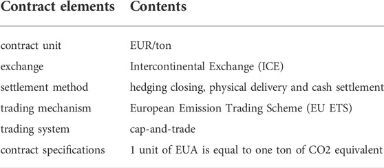
TABLE 1. EUA futures contract
However, due to the short implementation time of carbon trading system, the risk aversion mechanism is relatively scarce. In order to effectively capture the futures market risk, this paper plans to model and predict the volatility of EUA futures, so as to optimize the market risk management mechanism. In addition, when carbon emissions continue to increase, the climate often changes, leading to the continuous adjustment of subsequent policies. At this time, investors will pay more attention to the price fluctuation of carbon futures. Therefore, the price fluctuation of EUA futures in global climate is of great significance to market participants and political decision makers.
Byun and Cho (2013) find that the EUA futures price volatility will be affected by climate change and the adjustment of policy uncertainty. In fact, climate change and policy adjustments will exacerbate the volatility of carbon futures prices. First, from the perspective of demand, when the climate changes, residents’ demand for carbon products will increase. The increased consumption demand of carbon products will promote the production increase of enterprises, and the sales volume of carbon emission products will increase until the carbon emission reaches the upper limit, so as to speed up the development of the carbon market (Bertini et al., 2020). Secondly, from the perspective of supply, when the climate changes extremely, raw materials cannot be supplied in time, which leads to the rise of carbon emission costs. In order to reduce the cost of purchasing raw materials, enterprises will reduce carbon emissions. Finally, from the perspective of society, when climate change, supply and demand will be unbalanced, and the government will maintain the balance of carbon prices for society (van et al., 2019).
Moreover, in recent years, due to the uncertain changes of economic policies and the continuous emergence of the black swan event, various uncertain factors have been brought to the enterprises and decision makers among the actual traders. In this case, enterprises and decision makers tend to hold a conservative attitude and show risk aversion, which affects the price fluctuation of EUA futures (Chevallier, 2009, 2011; Zhu and Chevallier, 2017). In order to further explore the fluctuation of EUA futures, it is vital to accurately model and forecast the volatility of EUA futures.
In the past decades, many volatility methods have been proposed to model and forecast carbon price. Ren et al. (2022a) find the following conclusions after many studies. First, the yield of carbon futures will be affected by the Brent spot price, the closing price of United Kingdom crude oil and the growth of United Kingdom natural gas production under extreme conditions. Then, both Bitcoin and gold perform as weak hedges for oil portfolios. Final, the effects of the carbon futures in the medium to long term is positive and in the short term is instable. Wen et al. (2022) study the impulse response of gold, Bitcoin, oil and stock markets before and after the COVID-19, the results show that gold is a safe haven for oil and stock markets during the COVID-19 pandemic. What’s more, due to the simple structure and easy implementation, the generalized autoregressive conditional heteroscedasticity (GARCH) model proposed by Bollerslev (1986) becomes the most popular volatility model. As a consequence, many authors apply the GARCH model to predict EUA futures volatility, see, e.g., Byun and Cho (2013), Zeitlberger and Brauneis (2016), Wang et al. (2019), Naik et al. (2020), Huang et al. (2021). Later, some scholars expand GARCH model and construct TGARCH, GJR-GARCH, ARMAX-GARCH, STR-GARCH models to predict the volatility of carbon futures price (Arouri et al., 2012; Byun and Cho, 2013; Rannou and Barneto, 2016; Sheng et al., 2021). Despite the empirical success of GARCH-type models, they still only use the daily return information for forecasting EUA futures volatility, which ignores other information such as investor sentiment.
Actually, investor sentiment has broadly researched in financial markets like stock markets (Wen et al., 2019), FX markets (Han et al., 2018), commodity markets (Kou et al., 2018) and exchange rate markets (Perez-Liston et al., 2018) and has proved to be an influential pricing factor in these markets. Later, some authors study the impact of investor sentiment on the volatility of EUA futures. Benz et al. (2021) show that different types of investors have different preference for carbon intensive investments. Zhang et al. (2021) show that investor sentiment contains excellent explanatory information for forecasting carbon price. In general, the existing research shows that companies and investors will largely affect price fluctuations. On the one hand, investors are negatively correlated with carbon emissions (Riedl and Smeets, 2017; Benz et al., 2020; Bolton and Kacperczyk, 2021). On the other hand, investors are closely related to the company’s carbon risk management (Dyck et al., 2019). Since investor sentiment is closely related to risk appetite (Bams et al., 2017), it is reasonable to conjecture that risk aversion will have an important impact on the volatility of EUA futures. However, as far as we know, few studies have investigated the impact of risk aversion on the volatility of EUA futures. The main reason may be the lack of effective measurement of risk aversion.
Recently, Bekaert et al. (2022), under the dynamic non arbitrage asset pricing model, propose a time-varying risk aversion (RA) index based on six financial instruments, including the term spread, credit spread, a detrended earnings yields, realized and risk-neutral equity return variances, and the realized corporate bond return variances. Several studies have shown that the RA index contains information useful for predicting financial volatility. For example, Demirer et al. (2019) adopt the heterogeneous autoregressive realized volatility (HAR-RV) model to study the impact of RA index on the gold market volatility, and find that incorporating RA index can significantly improve forecasting accuracy for gold volatility. Dai and Chang (2021) use the linear regression method to investigate the predictive value of RA index over the volatility of the United States stock market. They find that RA index has a significant impact on the volatility of the United States stock market and can improve the prediction of out-of-sample volatility. However, there are few studies on studying the relation between time-varying risk aversion and EUA futures volatility. At the same time, whether time-varying risk aversion can predict EUA futures volatility has not been explored. In light of this, this paper studies the relation between time-varying risk aversion and EUA futures volatility, and explores the predictive value of time-varying risk aversion for the EUA futures volatility.
The standard GARCH model can not incorporate exogenous explanatory variables to describe the dynamics of energy volatility, and thus it can not adequately capture and predict the EUA futures volatility. Moreover, the frequency of exogenous explanatory variables are usually inconsistent with that of financial market data. To address the issue of mixed-frequency data, Ghysels et al. (2007) first introduce the mixed data sampling (MIDAS) model. Further, Engle et al. (2013) incorporate the MIDAS method into the GARCH model and propose the GARCH-MIDAS model. The most prominent feature of the GARCH-MIDAS model is that it decomposes the volatility into a short-term and a long-term components, where the short-term component follows the standard GARCH(1,1) process, while the long-term component is modeled by the MIDAS method with low-frequency variables.
Zhao et al. (2018) propose combination-MIDAS models to predict the weekly EUA futures price, the empirical results show that the combination-MIDAS models provide accurate forecasting performance and the coal contains more accurate information for EUA futures forecasting. Liu et al. (2021) use the GARCH-MIDAS model with economic policy uncertainty (EPU) to forecast the EUA futures volatility, and find that the GARCH-MIDAS model exhibit superior out-of-sample predictive ability. Dai et al. (2022) construct the GARCH-MIDAS-EUEPU and GARCH-MIDAS-GEPU models for investigating the impact of European and global economic policy uncertainty on the EUA futures volatility, they find that both European and global economic policy uncertainty will exacerbate the EUA futures return. Wu et al. (2022) forecast the EUA futures volatility using EGARCH-MIDAS model, and show that the EUA futures volatility exhibits a leverage effect and the proposed EGARCH-MIDAS model outperforms the traditional competing models. Guo et al. (2022) propose the GARCH-MIDAS-JUMP and GARCH-MIDAS-JUMP-LJ models for forecasting volatility of EUA futures, they find that both long-term and short-term asymmetries, extreme observations, and jump information have substantially effect on the EUA volatility.
Although GARCH-MIDAS model has achieved success in experience, it still has some shortcomings. For example, it still unable to capture the characteristics of time-varying higher moments (skewness and kurtosis) in the conditional distribution of financial returns. A large number of studies have shown that the return of EUA futures presents a skewed and heavy tailed distribution. Moreover, the skewness and kurtosis of EUA futures return change over time. That is, the distribution of EUA futures return presents the characteristics of time-varying higher moments (see, e.g., Amaya et al., 2015; De Luca and Loperfido, 2015; Fry-McKibbin and Hsiao, 2018; Yun et al., 2020). Recently, studies on EUA futures volatility modelling and forecasting emphasizes the importance of skewness and kurtosis. For example, Da Fonseca and Xu (2017) analyze the predictability of crude oil market excess returns by decomposed variance and skew risk premiums, and they find that the decomposed high moment risk premiums contain much more predictive information. Ioannidis et al. (2021) propose a periodic GARCH-M model with conditional skewness and kurtosis components, and apply it for electricity price data, the empirical results show that seasonality affects the time varying moments of the distribution. Zhang et al. (2022) investigate the asymmetric relations between returns and changes in implied moments (i.e., volatility, skewness, and kurtosis) in the crude oil market, the results show that preference higher moments theory and prospect theory provide relevant explanations of the contemporaneous return higher moments relation, and the return higher moments relation is asymmetric. Bouri et al. (2021) find that considering the spillover effect of higher moments and jumps has an impact on portfolio and risk management in many markets (such as United States stock, crude oil and gold markets). In addition, Mensi et al. (2022) represent to understand the asymmetric connectedness, spillovers in realized volatility as well as higher moments (realized skewness, kurtosis, etc. of the asset prices) between six popular currencies and crude oil markets, they find that these markets are strongly interconnected and the vast majority of the spillover of realized skewness in the seven currencies assets originate within their own markets. In fact, most of the current studies on EUA futures volatility do not consider the time-varying higher moments characteristics of EUA futures return distribution.
Motivated by the above insights, this paper extends the GARCH-MIDAS model to the GARCH-MIDAS with skewness and kurtosis (hereafter GARCH-MIDAS-SK model). The GARCH-MIDAS-SK model has the capacity to accommodate time-varying higher moments of financial return distribution. We apply the GARCH-MIDAS-SK model to monthly RA index and daily EUA futures data. The empirical results show that the GARCH-MIDAS-SK-RA model outperforms a variety of competing models, including the GARCH, GARCH-MIDAS, GARCH-MIDAS-RA and GARCH-MIDAS-SK models, in terms of out-of-sample EUA futures volatility forecasting for forecasting horizons of 1 day up to 22 days (1 month). Moreover, robustness analysis based on alternative out-of-sample forecasting windows confirms the superior predictive power of the GARCH-MIDAS-SK-RA model. The findings highlight the value of incorporating time-varying higher moments and RA for forecasting EUA futures volatility.
To sum up, this paper has the following innovation and contribution: First, the GARCH-MIDAS-SK framework that incorporates time-varying higher moments is proposed. Second, the relation between RA and the EUA futures volatility is investigated. Third, RA has a significantly negative impact on EUA futures volatility. Fourth, the EUA futures return distributions exhibit obvious features of time-varying higher moments. Fifth, both RA and time-varying higher moments capture predictive information over EUA futures volatility.
The remainder of the paper is organized as follows. In Section 2, we introduce the GARCH-MIDAS-SK model. In Section 3, we describe the method for evaluating volatility forecast accuracy. Section 4 presents the empirical results, while Section 5 concludes.
2 The model
2.1 GARCH mdoel
Bollerslev (1986) proposes the popular GARCH model to describe the dynamics of financial asset returns. The standard GARCH model is given by
where rt is the log return, μ is the conditional mean of the return,
2.2 GARCH-MIDAS model
The GARCH model only uses historical return information to model and forecast volatility, and ignores macroeconomic information. Generally, the sampling frequency of macroeconomic variables are different from the daily return (lower). The GARCH model cannot combine data sampled at different frequencies. To overcome this problem, Engle et al. (2013) propose the GARCH-MIDAS model, which can easily introduce macroeconomic variables (data sampled at a frequency different from the daily rate of return). The GARCH-MIDAS model is as follows
where ri,t is the log return on day i in period t (month).
It can be seen from Eq. 6 that conditional variance
where α + β < 1, which ensures the stationarity of short-term component gi,t.
The long-term component τt is specified by smoothing realized volatility (RV) using the MIDAS regression approach
where K is the number of MIDAS lags, φk (⋅) is a non-negative weighting function and RVt is the monthly RV, which is defined as
where Nt is the number of trading days in month t. Following Engle et al. (2013), Asgharian et al. (2016), Yu et al. (2018) and Li et al. (2020), we choose single-parameter Beta polynomial for the weighting function φk (⋅), which is given by
2.3 GARCH-MIDAS-SK model
It has been well documented in the literature that the distribution of financial returns usually shows the characteristics of time-varying higher moments (skewness and kurtosis) (see, e.g., Johnson, 2002; Carr and Wu, 2007; Bakshi et al., 2008). In order to capture this empirical feature of the financial returns data, we extend the GARCH-MIDAS model to incorporate time-varying skewness and kurtosis and propose the GARCH-MIDAS-SK model. To be specific, we assume that the return innovation ɛi,t follows the Gram-Charlier distribution with zero mean, unit variance, time-varying skewness si,t and kurtosis ki,t, that is,
where
We assume that the skewness si,t and kurtosis ki,t follow a GARCH (1,1) process, which conditionally depend on the historical return innovation ɛi−1,t. Therefore, the GARCH-MIDAS-SK model is given as follows
It is clear that the GARCH-MIDAS-SK model is a general and flexible model. In fact, it includes the GARCH-MIDAS model with the Gaussian innovation as a special case when si,t = 0 (γ0 = γ1 = γ2 = 0) and ki,t = 3 (δ0 = 3, δ1 = δ2 = 0).
2.4 Incorporating RA
The GARCH-MIDAS-SK model is flexible and can be easily extended to incorporate RA. This can be done by incorporating RA into the long-term component process
Equation 23 emphasizes the importance of RA in modelling the long-term volatility. We refer to the extended model as the GARCH-MIDAS-SK-RA model.
2.5 The maximum likelihood estimation
The parameters of the GARCH-MIDAS-SK model can be easily estimated by employing the classical maximum likelihood method. Specifically, the log likelihood function of the model can be written as
where
3 Evaluation of volatility forecasts
3.1 k-day-ahead forecast
On day i in month t, the k-day-ahead forecast λi+k,t|i based on the GARCH-MIDAS-SK model can be obtained as
where
It is worth pointing out here that the prediction of long-term component τt based on information set
3.2 Loss functions
Since the true volatility is unobservable, a proxy for the true volatility needs to be choosed when evaluating and comparing the volatility forecasting models. In the paper, the squared return
where pi,t is the EUA futures price on day i in month t.
In the paper, five loss functions, including the mean square error (MSE), mean absolute error (MAE), heteroscedasticity adjusted MSE (HMSE), heteroscedasticity adjusted MAE (HMAE) and quasi-likelihood (QLIKE), are employed to evaluate the accuracy of volatility forecasts. Among them, the MSE and QLIKE are robust loss functions (Patton, 2011). The five evaluation criteria are defined as
where L is the number of out-of-sample volatility forecasts,
3.3 MCS test
Further, the model confidence set (MCS) test proposed by Hansen et al. (2011) is employed to examine whether the differences in forecast accuracy among competing models are significant. To be specific, the MCS procedure relies on an equivalence test
where duv,i,t is the loss difference between model u and v. Hansen et al. (2011) propose the following MCS t-statistics to test the null hypothesis
where
3.4 DM test
The size of the loss function can be used as a standard to measure the prediction ability of the model, but it is impossible to determine whether the result is statistically significant. To solve this problem, Diebold and Mariano (1995) proposed DM statistics, which is suitable for the comparison between the two models. Specifically, first assume that the true value is {yt}, the predicted values of the two models are
The loss function is a function of the prediction error, expressed as
where, Lossi,t represents the loss function of Volatility Prediction of the ith model.
If the original assumption is that the two models have the same prediction ability, then the unconditional expectation of the loss function of the predicted values of the two models is 0, that is
where, dt = Loss1t − Loss2t represents the loss difference between models 1 and 2. Then, the corresponding alternative assumption: the prediction ability of model 1 is worse than that of model 2, that is
where,
where,
4 Empirical analysis
4.1 Data
For our empirical analysis, we use the data on the daily EUA futures returns and monthly RA index. Since EU ETS was established, EU ETS has been divided into four phases (phase I: from 3 January 2005 to 31 December 2007; phase II: from 2 January 2008 to 31 December 2012; phase III: from 2 January 2013 to 31 December 2020; phase IV, from 4 January 2021 to 31 December 2030). Due to the phase I is a trial stage, EU ETS was restricted in bank loan and resulted in the EUA futures price tends to be zero at the end of phase I (Tian et al., 2016). In view of this, the sample period for the EUA futures return data is from 2 January 2008 to 31 December 2021 (phase II to phase IV), resulting in 3,605 daily observations. The data are obtained from Wind database of China.
For the time-varying risk aversion, we use the time-varying risk aversion (RA) index proposed by Bekaert et al. (2022). The RA index can be obtained from the website https://www.nancyxu.net/risk-aversion-index. In order to be consistent with the sample period of the EUA futures returns, we choose the RA sample period from January 2008 to December 2021, resulting in a total of 168 monthly observations.
Figure 1 presents the time series plots of the daily EUA futures returns and the monthly RA index. It can be seen from the figure that the well-known behaviors of volatility clustering in the EUA futures are apparent. It is also worth noting that the EUA futures experienced significant fluctuations, particularly in recent years. As can be seen from the time series plot of RA, during the period of global financial crisis in 2008, the RA index increased significantly. Moreover, during the periods of 2011 U.S. debt crisis and the COVID-19 in 2020, the RA index also increases significantly. On the whole, the change of RA index is closely related to the overall international economic operation.
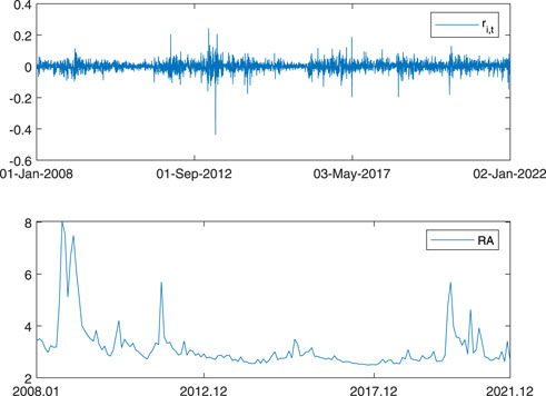
FIGURE 1. Time series plots of daily EUA futures returns and monthly RA index.
Table 2 reports the descriptive statistics of daily EUA futures returns (ri,t) and monthly RA index (RAt). As can be seen from the table, the daily EUA futures return series show the distribution of negative skewness (skewness smaller than 0) while the monthly RA index series show the distribution of positive skewness (skewness greater than 0) and both series show excess kurtosis (kurtosis greater than 3). Jarque-Bera statistics suggest that the series deviate from the normal distribution.

TABLE 2. Descriptive statistics.
4.2 Parameter estimation results
In order to implement the MIDAS models, we need to determine the lag length of MIDAS component, K. According to Conrad and Kleen (2020), as long as K is chosen large enough, the estimation results are robust to the choice of MIDAS lags K, since the Beta weighting function used in the paper is flexible and the data will identify the optimal weights. In view of this, we choose K = 36, i.e., three MIDAS lag years for the monthly explanatory variables. It is a common choice in the literature, which allows us to capture reasonable dynamics of long-term component (see, e.g., Engle et al., 2013; Asgharian et al., 2016; Conrad and Kleen, 2020). Using the maximum likelihood estimation method, the parameters of the GARCH, GARCH-MIDAS, GARCH-MIDAS-RA, GARCH-MIDAS-SK and GARCH-MIDAS-SK-RA models are estimated. The estimation results along with the standard errors, log-likelihood and Akaike information criterion (AIC) are presented in Table 3.
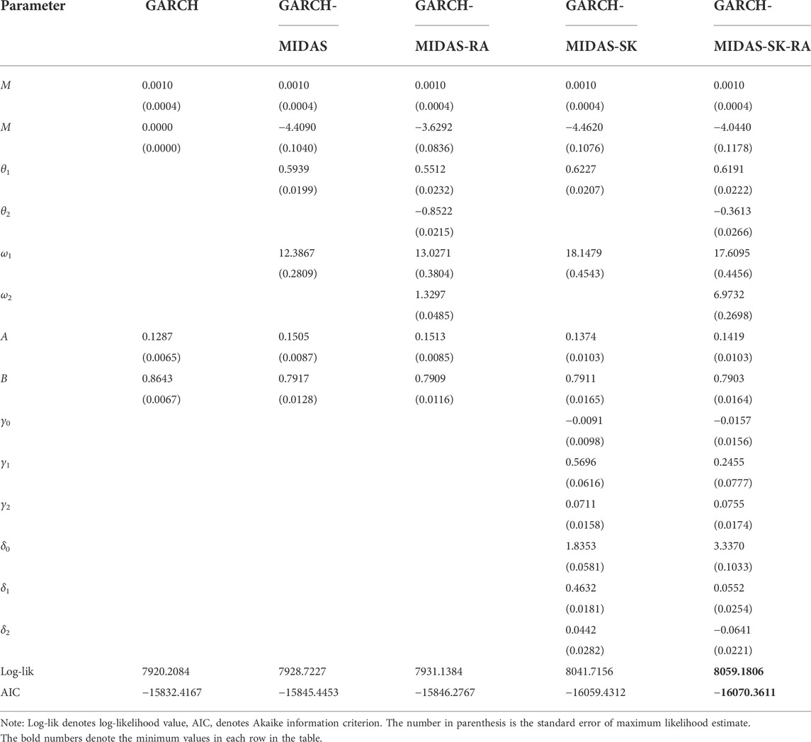
TABLE 3. Parameter estimation results.
As can be seen from Table 3, the persistence coefficient of GARCH model, α + β, is estimated to be very close to 1, indicating that the EUA futures return has high volatility persistence. In contrast, in the GARCH-MIDAS, GARCH-MIDAS-RA, GARCH-MIDAS-SK and GARCH-MIDAS-SK-RA models, the estimates of the persistence coefficient of short-term component, α + β, which are significantly lower than that in the GARCH model, indicating that the MIDAS structure is capable of capturing the long-term trend (long memory property) of the EUA futures volatility.
It is interesting to note that the estimates of the coefficient θ1 are all significantly positive, indicating that the monthly realized volatility (RV) has a significantly positive impact on the long-term volatility of EUA futures, that is, the monthly RV increases, the long-term volatility of EUA futures is expected to increase. While in the two MIDAS models incorporated RA (GARCH-MIDAS-RA model and GARCH-MIDAS-SK-RA model), the estimates of the coefficient θ2 are significantly negative, indicating that RA has a significantly negative impact on the long-term volatility of EUA futures, that is, an increase in RA level predicts higher level of long-term volatility of EUA futures. A possible explanation is that the dynamic determination of EUA futures can be expressed as the subjective belief of market participants in the future trend of EUA futures. When the carbon emission market is affected by emergencies, the risk aversion level of investors and regulatory authorities will be improved. In order to avoid the impact of special events and unexpected changes in the external environment, investors prefer sustainable mutual funds to stabilize the volatility of EUA futures despite low returns and high management fees. Therefore, a high level of risk aversion will reduce the long-term level of EUA futures volatility (Riedl and Smeets, 2017). Figure 2 shows the long-term component of the EUA futures volatility derived from the GARCH-MIDAS-SK-RA model. As can be seen from the figure, the long-term component is smooth and captures the long-term trend of the EUA futures volatility.
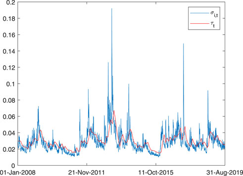
FIGURE 2. Long-term component of EUA futures volatility.
The GARCH-MIDAS-SK and GARCH-MIDAS-SK-RA models are able to capture the time-varying higher moments of return distribution. Turning to the skewness equation in the models, we find the evidence of the presence of time-varying skewness for the EUA futures returns, with the persistence coefficient (γ1) and shock coefficient (γ2) of skewness being significant. Regarding to the kurtosis equation, significant presence of time-varying kurtosis is also found for the EUA futures returns, with at least one of the persistence coefficient (δ1) and shock coefficient (δ2) being significant. Figure 3 plots the time-varying skewness and kurtosis of the EUA futures return estimated from the GARCH-MIDAS-SK-RA model. It can be seen intuitively from the figure that the conditional skewness and kurtosis series of EUA futures return have time-varying characteristics. Hence, it is necessary to prevent and avoid EUA futures risk from a dynamic perspective.
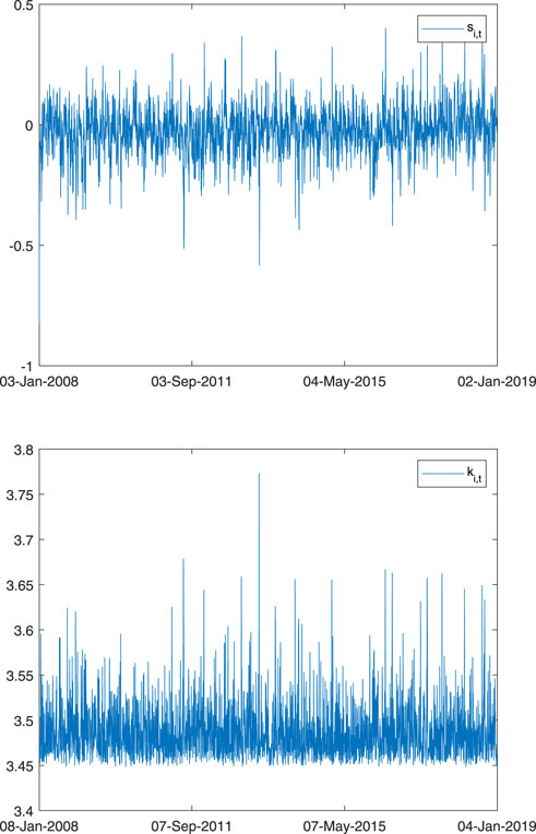
FIGURE 3. Time-varying skewness and kurtosis of EUA futures return.
Moreover, we can observe from Table 3 that the GARCH-MIDAS model outperforms the GARCH model in terms of the log-likelihood and AIC values. In particular, the GARCH-MIDAS-SK (GARCH-MIDAS-SK-RA) model outperforms the original GARCH-MIDAS (GARCH-MIDAS-RA) model, indicating that incorporating time-varying higher moments improves the empirical fit of the model. Overall, the GARCH-MIDAS-SK-RA model outperforms all other models.
4.3 Out-of-sample forecasting results
In order to investigate the predictive value of time-varying higher moments and RA for EUA futures volatility, we conduct an out-of-sample analysis by using the GARCH-MIDAS-SK-RA model. We compare the out-of-sample performance of the GARCH-MIDAS-SK-RA model with that of the GARCH, GARCH-MIDAS, GARCH-MIDAS-RA and GARCH-MIDAS-SK models. The rolling-window approach is employed to perform the out-of-sample forecast. To be specific, the full sample is splitted into two sub-samples: an in-sample period (2008.1.2–2018.12.28) and an out-of-sample period (2019.1.2–2021.12.31), in which the in-sample data (2,829 observations) are used to estimate the model parameters and the out-of-sample data (776 observations) are used to evaluate the out-of-sample forecasting performance. We first estimate the models using the first 2,829 observations to make k-day-ahead forecast. Then we roll the estimation sample forward daily (with a fixed window size of 2,829), and re-estimate the models and make new k-day-ahead forecast. The procedure is conducted repeatedly until the end of the sample. We compare the out-of-sample performance of different volatility models for forecasting horizons k = 1, 5, 10 and 22, i.e., 1-day, 5-days, 10-days and 22-days ahead forecasts.
Table 4 presents the out-of-sample forecasting results of the five models for forecasting the EUA futures volatility. It can be seen from Table 4 that the models with MIDAS structure (GARCH-MIDAS, GARCH-MIDAS-RA, GARCH-MIDAS-SK and GARCH-MIDAS-SK-RA models) produce more accurate volatility forecasts compared to the GARCH model in terms of the MSE, MAE, HMSE, HMAE and QLIKE criteria, indicating that incorporating long-term component (MIDAS structure) plays an important role in EUA futures volatility forecasting. In addition, both the GARCH-MIDAS-RA and GARCH-MIDAS-SK models generally outperform the original GARCH-MIDAS model. This result suggests that the incorporation of RA and time-varying higher moments can improve the forecasting accuracy of EUA futures volatility. In particular, we observe that the loss function values for the GARCH-MIDAS-SK model are lower than that of the GARCH-MIDAS-RA model, which suggests that incorporating time-varying higher moments is more important than incorporating RA for forecasting EUA futures volatility. Last but not least, the GARCH-MIDAS-SK-RA model that incorporates time-varying higher moments and RA offers the lowest loss values in all cases. This result highlights the value of introducing time-varying higher moments and RA in modeling and forecasting EUA futures volatility.
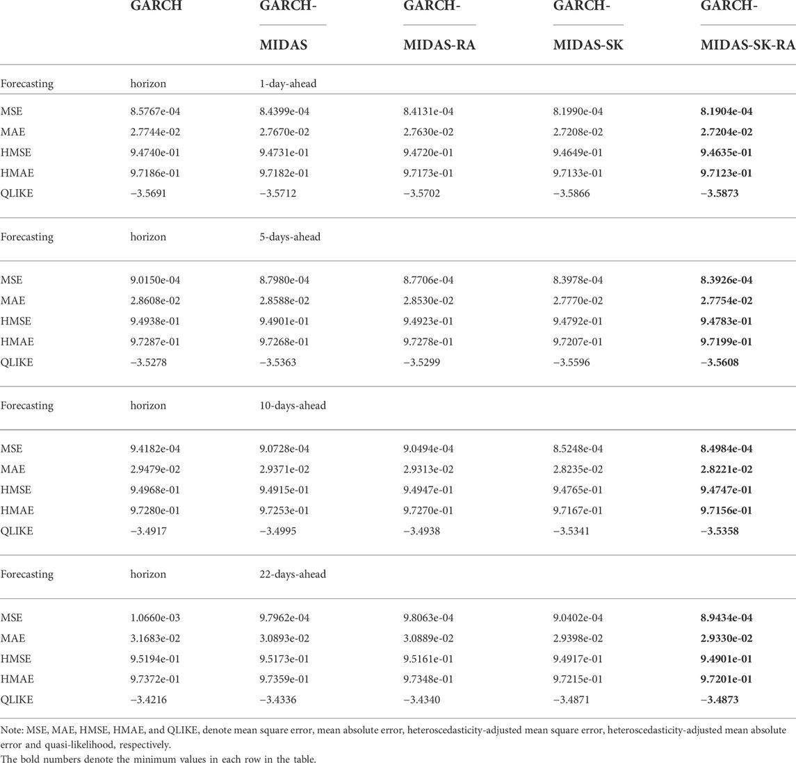
TABLE 4. Out-of-sample forecasting results.
Table 5 presents the MCS test results for the five models. As can be seen from Table 5, the GARCH, GARCH-MIDAS, GARCH-MIDAS-RA models are kicked out of the MCS in all cases (MCS p value is less than 0.1), while the GARCH-MIDAS-SK and the GARCH-MIDAS-SK-RA model is always included in the MCS. In particular, the GARCH-MIDAS-SK-RA model offers the highest MCS p value (p = 1) in all cases, suggesting that the GARCH-MIDAS-SK-RA model significantly outperforms all other models for forecasting the EUA futures volatility.
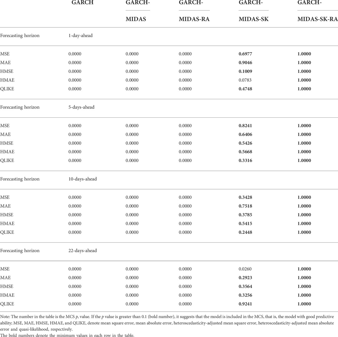
TABLE 5. MCS test results.
For the sake of further investigate whether the prediction ability of GARCH-MIDAS-SK-RA model changes in different periods, we first simply divide the sample into crisis period and non crisis period. We define the systemic crisis period as 2008–2009, and the data of all remaining years are classified as non-crisis. For the divided samples, we conduct MCS test again for crisis period and non-crisis period respectively, the results are shown on Tables 6 and 7. From the tables, we can also find that the GARCH-MIDAS-SK-RA model significantly outperforms all other models for forecasting the EUA futures volatility whether in crisis period or non-crisis period.
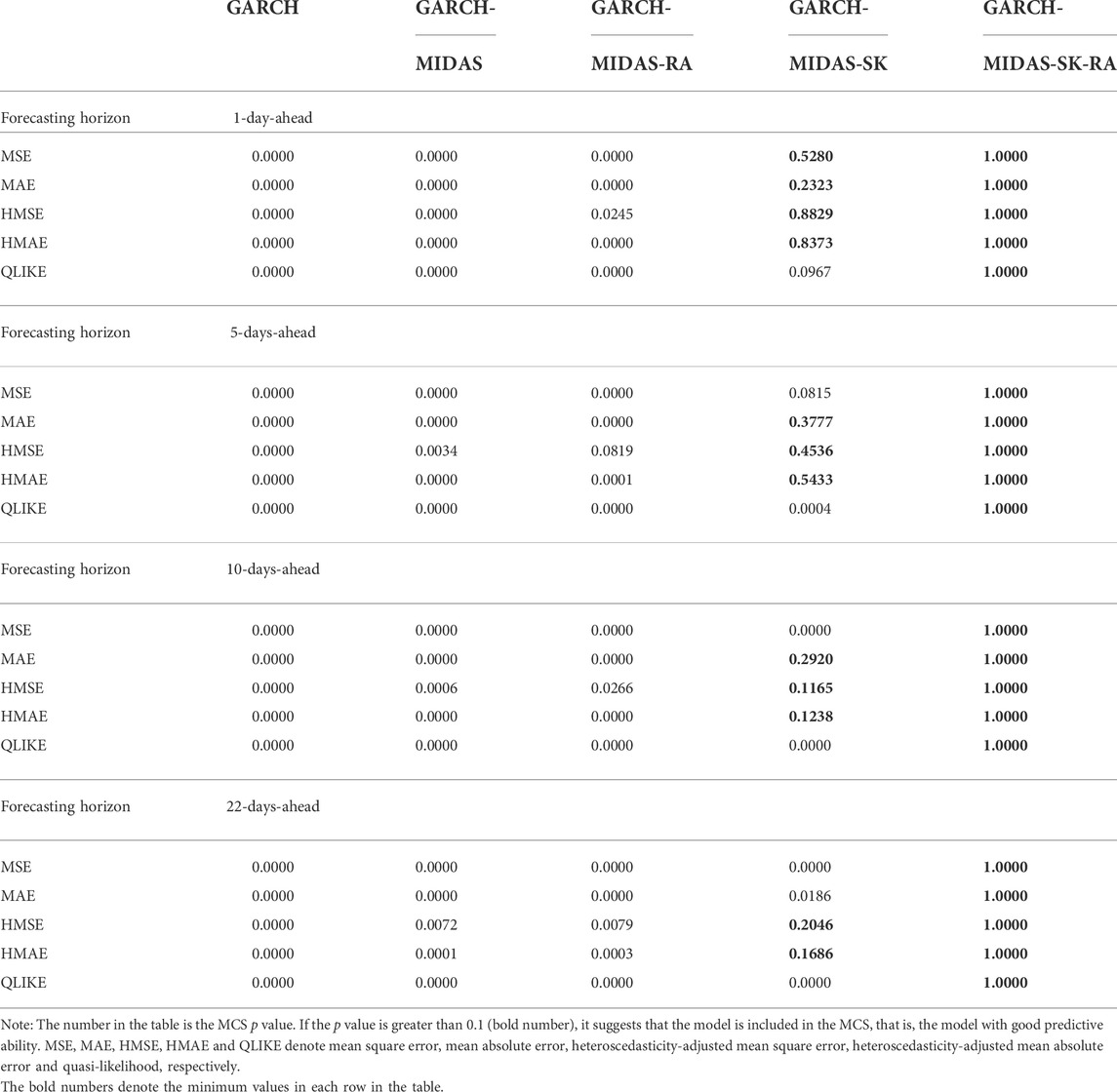
TABLE 6. MCS test results (in crisis period).
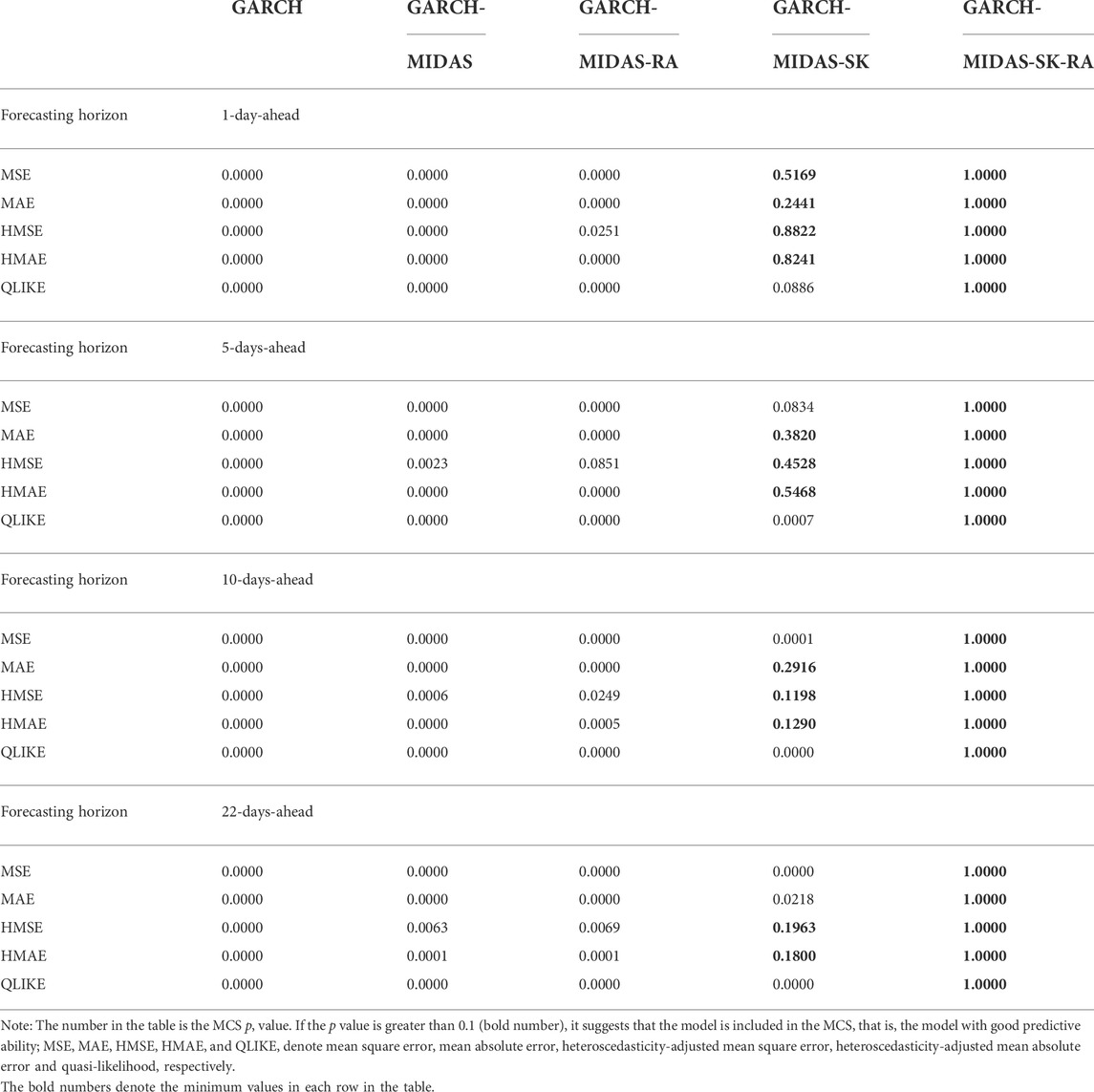
TABLE 7. MCS test results (in non-crisis period).
4.4 Robustness checks
In order to test the robustness of the out-of-sample results, we further consider alternative forecasting windows (out-of-sample periods) of 500 and 1,000. The out-of-sample results are presented in Tables 8 and 9.
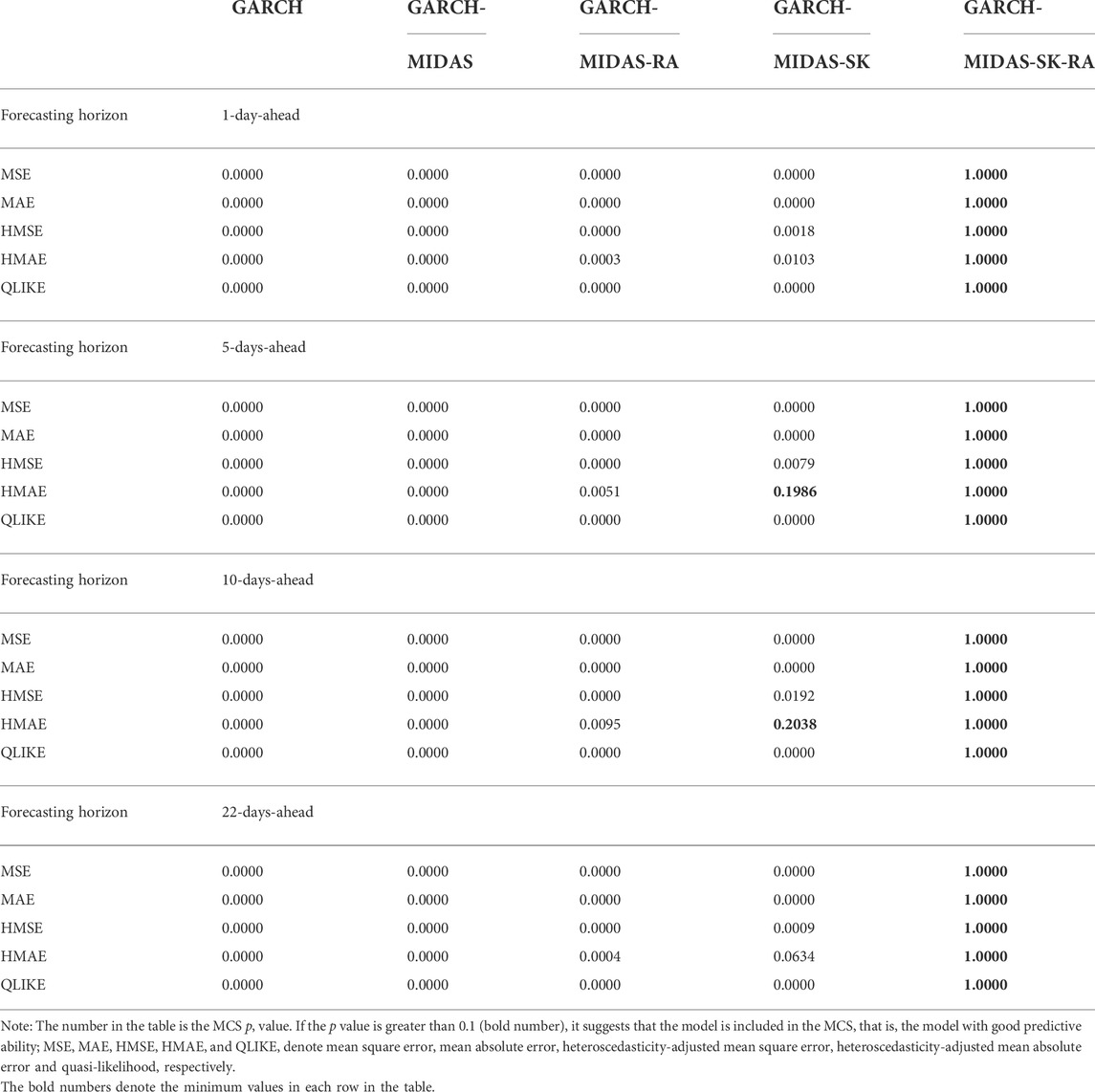
TABLE 8. MCS test results (alternative forecasting window of 500).
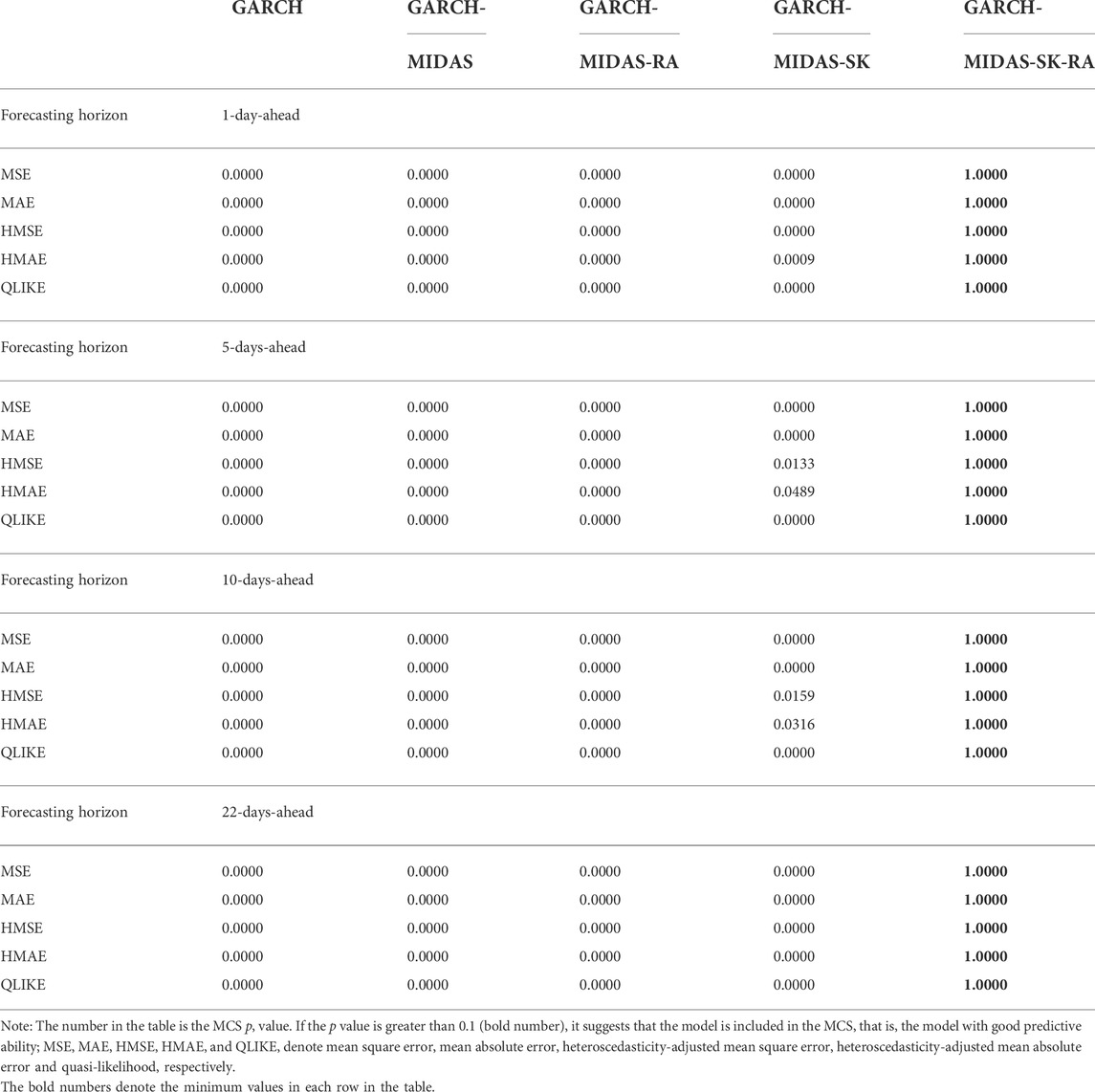
TABLE 9. MCS test results (alternative forecasting window of 1,000).
It can be seen from Tables 8 and 9 that the GARCH-MIDAS-SK-RA model that incorporates time-varying higher moments and RA significantly outperforms all other models in forecasting the volatility of EUA futures, which is consistent with the results reported in Table 5. The results suggest that the superior predictive power of the GARCH-MIDAS-SK-RA model is robust to alternative forecasting windows.
For the sake of enhancing the robustness of the test, DM test is carried out in this paper, and the test results are shown in Table 10. Compared with other models, the DM test results of GARCH-MIDAS-SK-RA model are significant, indicating that GARCH-MIDAS-SK-RA model is significantly better than the other four models in terms of prediction, this is consistent with the conclusions in Tables 5–10.
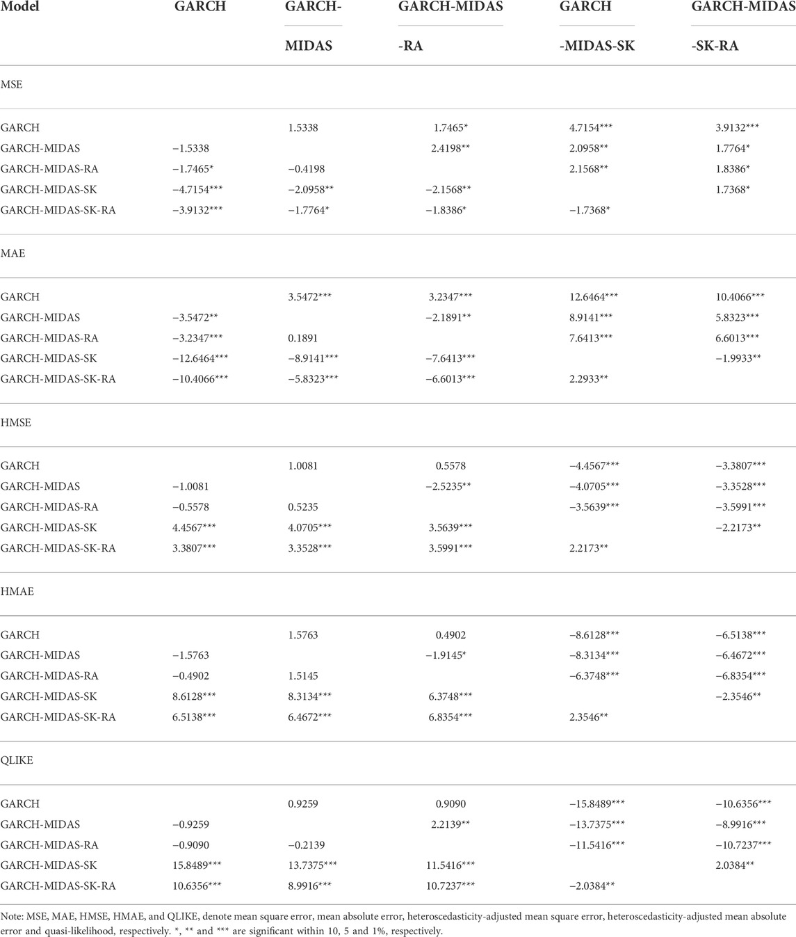
TABLE 10. DM test results.
5 Conclusion
In this paper, we investigate the predictive value of the time-varying higher moments and RA for the EUA futures volatility. We extend the GARCH-MIDAS model to incorporate time-varying skewness and kurtosis and propose the GARCH-MIDAS-SK model to model and forecast the EUA futures volatility. An empirical application to monthly RA index and daily EUA futures returns shows that the EUA futures volatility exhibits the characteristics of time-varying higher moments and RA has a significantly negative impact on the long-term volatility of EUA futures. Moreover, the GARCH-MIDAS-SK-RA model outperforms many competing models, including the GARCH, GARCH-MIDAS, GARCH-MIDAS-RA and GARCH-MIDAS-SK models in terms of out-of-sample forecast performance for forecast horizons of 1 day up to 1 month (22 days). In addition, the superior predictive power of the GARCH-MIDAS-SK-RA model is robust to alternative out-of-sample forecasting windows. The findings highlight the value of incorporating time-varying higher moments and RA for forecasting EUA futures volatility.
According to the research conclusion, we put forward the following suggestions: First, the state should formulate a reasonable trading mechanism and carbon quota agreement, improve the fluctuation of EUA futures trading price by changing the supply of carbon emission trading market, and improve the activity of carbon market while safeguarding the rights and interests of investors. Second, the government should strengthen the supervision of the market, carry out risk control and price adjustment intervention on the market by financial means, constantly adjust the market structure, standardize the trading system, and provide a way for investors to avoid risks, so as to prevent excessive fluctuations in EUA futures trading prices and affect the stability of the EUA futures trading market. Third, relevant departments should do a good job in the connection and transition between various regions and the national carbon emission market, expand the market scale and industry access scope, and promote the steady construction of the national EUA futures trading market.
The study provides a promising approach for modeling and forecasting EUA futures volatility, which is of great importance for both academic researchers and practical practitioners. It is worth pointing out that the research work can be extended. For example, the leverage effect could be incorporated into the GARCH-MIDAS-SK framework, which has been proved to be useful for improving the accuracy of volatility forecasts.
Data availability statement
The original contributions presented in the study are included in the article/Supplementary Material, further inquiries can be directed to the corresponding author.
Author contributions
XW: Conceptualization, Methodology, Formal analysis, Supervision. XM: Data curation, Software, Validation, Writing -review; editing. ZD: Writing -original draft, Funding acquisition.
Funding
This work was supported by the National Natural Science Foundation of China under Grant No. 71971001; Anhui University Collaborative Innovation Project under Grant No. GXXT-2021-078; Innovative Research Project for Graduates of Anhui University of Finance and Economics under Grant No. ACYC2020185; University Research Project for Graduates of Anhui Province under Grant No. YJS20210420.
Conflict of interest
The authors declare that the research was conducted in the absence of any commercial or financial relationships that could be construed as a potential conflict of interest.
Publisher’s note
All claims expressed in this article are solely those of the authors and do not necessarily represent those of their affiliated organizations, or those of the publisher, the editors and the reviewers. Any product that may be evaluated in this article, or claim that may be made by its manufacturer, is not guaranteed or endorsed by the publisher.
References
Amaya, D., Christoffersen, P., Jacobs, K., and Vasquez, A. (2015). Does realized skewness predict the cross-section of equity returns? J. Financial Econ. 118 (1), 135–167. doi:10.1016/j.jfineco.2015.02.009
Arouri, M. E. H., Jawadi, F., and Nguyen, D. K. (2012). Nonlinearities in carbon spot-futures price relationships during Phase II of the EU ETS. Econ. Model. 29 (3), 884–892. doi:10.1016/j.econmod.2011.11.003
Asgharian, H., Christiansen, C., and Hou, A. J. (2016). Macro-finance determinants of the long-run stock-bond correlation: The DCC-MIDAS specification. J. Financial Econ. 14 (3), 617–642. doi:10.1093/jjfinec/nbv025
Bakshi, G., Carr, P., and Wu, L. (2008). Stochastic risk premiums, stochastic skewness in currency options, and stochastic discount factors in international economies. J. Financial Econ. 87 (1), 132–156. doi:10.1016/j.jfineco.2006.12.001
Bams, D., Honarvar, I., and Lehnert, T., 2017. Risk aversion, sentiment and the cross-section of stock returns. Working Paper Limburg Institute of Financial Economics (LIFE).
Bekaert, G., Engstrom, E. C., and Xu, N. R. (2022). The time variation in risk appetite and uncertainty. Manag. Sci. 68, 3975–4004. doi:10.1287/mnsc.2021.4068
Benz, L., Jacob, A., Paulus, S., and Wilkens, M. (2020). Herds on green meadows: The decarbonization of institutional portfolios. J. Asset Manag. 21 (1), 13–31. doi:10.1057/s41260-019-00147-z
Benz, L., Paulus, S., Scherer, J., Syryca, J., and Truck, S. (2021). Investors’ carbon risk exposure and their potential for shareholder engagement. Bus. Strategy Environ. 30 (1), 282–301. doi:10.1002/bse.2621
Bertini, M., Buehler, S., Halbheer, D., and Lehmann, D. R. (2020). Carbon Foot printing and pricing under climate concerns. J. Mark. 86, 186–201. doi:10.1177/0022242920932930
Bollerslev, T. (1986). Generalized autoregressive conditional heteroskedasticity. J. Econ. 31 (3), 307–327. doi:10.1016/0304-4076(86)90063-1
Bolton, P., and Kacperczyk, M. (2021). Do investors care about carbon risk? J. Financial Econ. 142 (2), 517–549. doi:10.1016/j.jfineco.2021.05.008
Bouri, E., Lei, X., Jalkh, N., Xu, Y., and Zhang, H. (2021). Spillovers in higher moments and jumps across US stock and strategic commodity markets. Resour. Policy 72, 102060. doi:10.1016/j.resourpol.2021.102060
Byun, S. J., and Cho, H. (2013). Forecasting carbon futures volatility using GARCH models with energy volatilities. Energy Econ. 40, 207–221. doi:10.1016/j.eneco.2013.06.017
Carr, P., and Wu, L. (2007). Stochastic skew in currency options. J. Financial Econ. 86 (1), 213–247. doi:10.1016/j.jfineco.2006.03.010
Chevallier, J. (2011). A model of carbon price interactions with macroeconomic and energy dynamics. Energy Econ. 33 (6), 1295–1312. doi:10.1016/j.eneco.2011.07.012
Chevallier, J. (2009). Carbon futures and macroeconomic risk factors: A view from the EU ETS. Energy Econ. 31 (4), 614–625. doi:10.1016/j.eneco.2009.02.008
Conrad, C., and Kleen, O. (2020). Two are better than one: Volatility forecasting using multiplicative component GARCH-MIDAS models. J. Appl. Econ. Chichester. Engl. 35 (1), 19–45. doi:10.1002/jae.2742
Da Fonseca, J., and Xu, Y. (2017). Higher moment risk premiums for the crude oil market: A downside and upside conditional decomposition. Energy Econ. 67, 410–422. doi:10.1016/j.eneco.2017.08.024
Dai, P. F., Xiong, X., Duc Huynh, T. L., and Wang, J. (2022). The impact of economic policy uncertainties on the volatility of European carbon market. J. Commod. Mark. 26, 100208. doi:10.1016/j.jcomm.2021.100208
Dai, Z., and Chang, X. (2021). Forecasting stock market volatility: Can the risk aversion measure exert an important role? North Am. J. Econ. Finance 58, 101510. doi:10.1016/j.najef.2021.101510
De Luca, G., and Loperfido, N. (2015). Modelling multivariate skewness in financial returns: A SGARCH approach. Eur. J. Finance 21 (13-14), 1113–1131. doi:10.1080/1351847x.2011.640342
Demirer, R., Gkillas, K., Gupta, R., and Pierdzioch, C. (2019). Time-varying risk aversion and realized gold volatility. North Am. J. Econ. Finance 50, 101048. doi:10.1016/j.najef.2019.101048
Diebold, F. X., and Mariano, R. S. (1995). Comparing predictive accuracy. J. Bus. Econ. Stat. 13 (3), 253–263. doi:10.1080/07350015.1995.10524599
Dominicy, Y., and Vander Elst, H., 2015. Macro-driven VaR forecasts: From very high to very low-frequency data. Available at SSRN 2701256.
Dyck, A., Lins, K. V., Roth, L., and Wagner, H. F. (2019). Do institutional investors drive corporate social responsibility? International evidence. J. Financial Econ. 131 (3), 693–714. doi:10.1016/j.jfineco.2018.08.013
Engle, R. F., Ghysels, E., and Sohn, B. (2013). Stock market volatility and macroeconomic fundamentals. Rev. Econ. Statistics 95 (3), 776–797. doi:10.1162/rest_a_00300
Fry-McKibbin, R., and Hsiao, C. Y. L. (2018). Extremal dependence tests for contagion. Econ. Rev. 37 (6), 626–649. doi:10.1080/07474938.2015.1122270
Ghysels, E., Sinko, A., and Valkanov, R. (2007). MIDAS regressions: Further results and new directions. Econ. Rev. 26 (1), 53–90. doi:10.1080/07474930600972467
Guo, X., Huang, Y., Liang, C., and Umar, M. (2022). Forecasting volatility of EUA futures: New evidence. Energy Econ. 110, 106021. doi:10.1016/j.eneco.2022.106021
Han, L., Xu, Y., and Yin, L. (2018). Does investor attention matter? The attention-return relationships in FX markets. Econ. Model. 68, 644–660. doi:10.1016/j.econmod.2017.06.015
Hansen, P. R., Lunde, A., and Nason, J. M. (2011). The model confidence set. Econometrica 79 (2), 453–497.
Huang, Y., Dai, X., Wang, Q., and Zhou, D. (2021). A hybrid model for carbon price forecasting using GARCH and long short-term memory network. Appl. Energy 285, 116485. doi:10.1016/j.apenergy.2021.116485
Ioannidis, F., Kosmidou, K., Savva, C., and Theodossiou, P. (2021). Electricity pricing using a periodic GARCH model with conditional skewness and kurtosis components. Energy Econ. 95, 105110. doi:10.1016/j.eneco.2021.105110
Johnson, T. C. (2002). Volatility, momentum, and time-varying skewness in foreign exchange returns. J. Bus. Econ. Statistics 20 (3), 390–411. doi:10.1198/073500102288618522
Kou, Y., Ye, Q., Zhao, F., and Wang, X. (2018). Effects of investor attention on commodity futures markets. Finance Res. Lett. 25, 190–195. doi:10.1016/j.frl.2017.10.014
Li, T., Ma, F., Zhang, X., and Zhang, Y. (2020). Economic policy uncertainty and the Chinese stock market volatility: Novel evidence. Econ. Model. 87, 24–33. doi:10.1016/j.econmod.2019.07.002
Liu, J., Zhang, Z., Yan, L., and Wen, F. (2021). Forecasting the volatility of EUA futures with economic policy uncertainty using the GARCH-MIDAS model. Financ. Innov. 7 (1), 76–19. doi:10.1186/s40854-021-00292-8
Mensi, W., Shafiullah, M., Vo, X., V., and Kang, S. H. (2022). Asymmetric spillovers and connectedness between crude oil and currency markets using high-frequency data. Resour. Policy 77, 102678. doi:10.1016/j.resourpol.2022.102678
Naik, N., Mohan, B. R., and Jha, R. A. (2020). GARCH-model identification based on performance of information criteria. Procedia Comput. Sci. 171, 1935–1942. doi:10.1016/j.procs.2020.04.207
OToole, C., and Slaymaker, R. (2021). Repayment capacity, debt service ratios and mortgage default: An exploration in crisis and non-crisis periods. J. Bank. Finance 133, 106271. doi:10.1016/j.jbankfin.2021.106271
Patton, A. (2011). Volatility forecast comparison using imperfect volatility proxies. J. Econ. 160 (1), 246–256. doi:10.1016/j.jeconom.2010.03.034
Perez-Liston, D., Huerta-Sanchez, D., and Gutierrez, J. (2018). Do domestic sentiment and the spillover of US investor sentiment impact Mexican stock market returns. J. Emerg. Mark. Finance 17 (2), S185–S212. doi:10.1177/0972652718777062
Rannou, Y., and Barneto, P. (2016). Futures trading with information asymmetry and OTC predominance: Another look at the volume/volatility relations in the European carbon markets. Energy Econ. 53, 159–174. doi:10.1016/j.eneco.2014.10.010
Ren, X., Duan, K., Tao, L., Shi, Y., and Yan, C. (2022a). Carbon prices forecasting in quantiles. Energy Econ. 108, 105862. doi:10.1016/j.eneco.2022.105862
Ren, X., Li, Y., Wen, F., and Lu, Z. (2022c). The interrelationship between the carbon market and the green bonds market: Evidence from wavelet quantile-on-quantile method. Technol. Forecast. Soc. Change 179, 121611. doi:10.1016/j.techfore.2022.121611
Ren, X., Wang, R., Duan, K., and Chen, J. (2022b). Dynamics of the sheltering role of Bitcoin against crude oil market crash with varying severity of the COVID-19: A comparison with gold. Res. Int. Bus. Finance 62, 101672. doi:10.1016/j.ribaf.2022.101672
Riedl, A., and Smeets, P. (2017). Why do investors hold socially responsible mutual funds. J. Finance 72 (6), 2505–2550. doi:10.1111/jofi.12547
Sheng, C., Zhang, D., Wang, G., and Huang, Y. (2021). Research on risk mechanism of Chinas carbon financial market development from the perspective of ecological civilization. J. Comput. Appl. Math. 381, 112990. doi:10.1016/j.cam.2020.112990
Tian, Y., Akimov, A., Roca, E., and Wong, V. (2016). Does the carbon market help or hurt the stock price of electricity companies? Further evidence from the European context. J. Clean. Prod. 112, 1619–1626. doi:10.1016/j.jclepro.2015.07.028
van, D., Ploeg, F., and de Zeeuw, A. (2019). Pricing carbon and adjusting capital to fend off climate catastrophes. Environ. Resour. Econ. (Dordr). 72, 29–50. doi:10.1007/s10640-018-0231-2
Wang, L., Tang, L., Qiu, X. M., Zhang, X. X., and Ma, R. H. (2019). The risk measurement of chinas carbon financial market: Based on GARCH and VaR model. Appl. Ecol. Environ. Res. 17 (4), 9301–9315. doi:10.15666/aeer/1704_93019315
Wen, F., Tong, X., and Ren, X. (2022). Gold or Bitcoin, which is the safe haven during the COVID-19 pandemic. Int. Rev. Financial Analysis 81, 102121. doi:10.1016/j.irfa.2022.102121
Wen, F., Xu, L., Ouyang, G., and Kou, G. (2019). Retail investor attention and stock price crash risk: Evidence from China. Int. Rev. Financial Analysis 65, 101376. doi:10.1016/j.irfa.2019.101376
Wu, X., Yin, X., and Mei, X. (2022). Forecasting the volatility of European Union allowance futures with climate policy uncertainty using the EGARCH-MIDAS Model. Sustainability 14 (7), 4306. doi:10.3390/su14074306
Yu, H., Fang, L., and Sun, W. (2018). Forecasting performance of global economic policy uncertainty for volatility of Chinese stock market. Phys. A Stat. Mech. its Appl. 505, 931–940. doi:10.1016/j.physa.2018.03.083
Yun, P., Zhang, C., Wu, Y., Yang, X., and Wagan, Z. A. (2020). A novel extended higher-order moment multi-factor framework for forecasting the carbon price: Testing on the multilayer long short-term memory network. Sustainability 12 (5), 1869. doi:10.3390/su12051869
Zeitlberger, A., and Brauneis, A. (2016). Modeling carbon spot and futures price returns with GARCH and Markov switching GARCH models. Cent. Eur. J. Oper. Res. 24 (1), 149–176. doi:10.1007/s10100-014-0340-0
Zhang, X., Bouri, E., Xu, Y., and Zhang, G. (2022). The asymmetric relationship between returns and implied higher moments: Evidence from the crude oil market. Energy Econ. 109, 105950. doi:10.1016/j.eneco.2022.105950
Zhang, Y., Chen, Y., Wu, Y., and Panpan, Z. (2021). Investor attention and carbon return: Evidence from the EU-ETS. Econ. Research-Ekonomska Istraivanja 2021, 1–19.
Zhao, X., Han, M., Ding, L., and Kang, W. (2018). Usefulness of economic and energy data at different frequencies for carbon price forecasting in the EU ETS. Appl. Energy 216, 132–141. doi:10.1016/j.apenergy.2018.02.003
Keywords: European Union allowance futures, time-varying higher moments, time-varying risk aversion, GARCH-MIDAS-SK model, forecasting
Citation: Wu X, Mei X and Ding Z (2022) Forecasting the volatility of European Union allowance futures with time-varying higher moments and time-varying risk aversion. Front. Environ. Sci. 10:973438. doi: 10.3389/fenvs.2022.973438
Received: 20 June 2022; Accepted: 18 July 2022;
Published: 11 August 2022.
Edited by:
Elie Bouri, Lebanese American University, LebanonReviewed by:
Xiaohang Ren, Central South University, ChinaYahua Xu, Central University of Finance and Economics, China
Copyright © 2022 Wu, Mei and Ding. This is an open-access article distributed under the terms of the Creative Commons Attribution License (CC BY). The use, distribution or reproduction in other forums is permitted, provided the original author(s) and the copyright owner(s) are credited and that the original publication in this journal is cited, in accordance with accepted academic practice. No use, distribution or reproduction is permitted which does not comply with these terms.
*Correspondence: Xueting Mei, bV94dWV0aW5nQDE2My5jb20=