 M. van den Berg
 S. J. H. Rikkert1
- 1Coastal Engineering Section, Hydraulic Engineering Department, Delft University of Technology, Delft, Netherlands
- 2Environmental Fluid Mechanics Section, Hydraulic Engineering Department, Delft University of Technology, Delft, Netherlands
Coastal flood risk is expected to increase due to climate change and population growth. Much of our coastlines is protected by “grey” infrastructure such as a dike. Dike maintenance and strengthening requires ever increasing capital and space, putting their economic viability in question. To combat this trend, more sustainable alternatives are explored, also known as Nature based Solutions. A promising option has shown to be tidal marshes. Tidal marshes are coastal wetlands with high ecological and economic value. Also, they protect dikes through wave attenuation and in case of a dike breach reduce its development. However, the effectiveness of a tidal marsh on reducing dike breach development rates highly depends on the stability of the tidal marsh itself. Not much is known about the stability of a tidal marsh under dike breach conditions, which are accompanied with flow velocities that can reach 4–5 m s−1. In this study we tested the vegetation response and erodibility of a mature tidal marsh, in-situ, under high flow velocities (
1 Introduction
A Low Elevation Coastal Zones (LECZ) is defined by McGranahan et al. (2007) as “contiguous area along the coast that is
Meanwhile, LECZs experience increased flood risk due to climate change induced sea level rise, increased storm intensity associated storm surges and ongoing land subsidence. Sea level rise causes the frequency of extreme water levels to double in the Tropics by 2030 (Vitousek et al., 2017), and doubles the odds of exceeding 50-year extreme water levels every 5 years along the U.S. coast (Taherkhani et al., 2020). Global extreme sea level projections show current 100-year extreme sea levels to be annual in the tropics by 2100 (Vousdoukas et al., 2018). At the same time, land subsidence compounds to flood risk as more area is susceptible to flooding (Shirzaei et al., 2020; Johnston et al., 2021; Nicholls et al., 2021; Fang et al., 2022; Tay et al., 2022). Besides, global coastal overtopping has already occurred 50% more often between 1993 and 2015 and is expected to accelerate faster throughout the 21st century (Almar et al., 2021). Kirezci et al. (2020) estimate that without coastal defences or adaptation measures an estimated 2.5%–4.1% of the global population will be at risk of flooding by a 100-year returning periodic event by 2100 under RCP8.5, which is 50% more than present day. Moreover, they mention that for most of the world, a 1 in a 100-year flood event could occur as frequently as once in 10 years by 2100. Although coastal defences are already built in many places and by 2100 coastal protection measures are likely widespread, this does highlight the scale and necessity of adapting current coastal protection strategies for such scenarios.
Much of the (urban) coastlines in LECZs is protected by hard “grey” flood defence structures such as dams, dikes, seawalls and storm surge barriers. A good example is the Netherlands which in 2000 had a total of 12 million people living in a LECZ (74% of its total population) ranking it third in the world (McGranahan et al., 2007). In the Netherlands a total of 3400 km of dunes, dams and dikes protect 60% of the country’s land which would otherwise be (regularly) flooded by sea, rivers and lakes. Apart from dunes, which is not a “grey” structure, this highlights the reliance of population in some LECZs on “grey” flood defences. Furthermore, continuous maintenance of these conventional flood defences is increasingly costly and typical strengthening of dikes (heightening and widening) becomes spatially or financially unfeasible. Much of the land side of dikes is already in use (urban, rural and industrial land use), while expansion at the water side is not always possible due to the presence of shipping channels, protected nature, or construction limits. Where space is available, instead of conventional strengthening more sustainable methods for flood protection are explored where nature is given more emphasis. These solutions are referred to as Nature based Solutions (NbS). Nature based Solutions aim to first understand the biophysical, socioeconomic and governmental aspects of systems. This leads to more balanced and resilient solutions (Temmerman et al., 2013).
One of the most promising NbS to flood protection is a tidal marsh. Tidal marshes are a type of coastal wetland (amongst intertidal flats, seagrass meadows and mangrove forests) characterised by their elevation (around mean high water) and frequent tidal flooding. Globally, an estimated 50% of the coastal wetland area has been lost since 1900 and 87% since 1700 (Davidson, 2014; Scott et al., 2014). Anthropogenic impacts such as land reclamation, sediment supply deprivation (fluvial dams) and accelerated sea level rise have been identified as main contributors to this loss (Scott et al., 2014). Also, decades of coastal squeeze (Pontee, 2013) by flood defence infrastructure has led to drowning of coastal wetlands. Most of the area loss occurred while the value of coastal wetlands (tidal marshes in particular) to ecosystems was largely unknown (Gedan et al., 2009). Barbier et al. (2011) identified seven ecosystem services by tidal marshes: biodiversity, erosion control, water purification, maintenance of fisheries, carbon sequestration, coastal protection and tourism, recreation, education and research. Moreover, salt marshes have the ability to grow with sea level rise via sediment accretion (Stralberg et al., 2011; Morris et al., 2016; Mitchell et al., 2017; Horton et al., 2018; Saintilan et al., 2022). The same studies also show that tidal marshes are vulnerable when sea level rise rates exceed the maximum accretion rate. However, Kirwan et al. (2016) argue that this vulnerability is often overestimated as the used process-based models do not capture biophysical feedback processes and inland migration. Different rehabilitation techniques exist to stimulate tidal marsh development. These typically focus either on vegetation (planting pioneer vegetation and invasive species control), modifying local hydrodynamics (tidal exchange and wave climate), creating land (using dredges materials or enhancing sediment accumulation) or a combination (managed realignment) (Billah et al., 2022). The success of such techniques highly depends on identifying causes, opportunities and proper evaluation (Waltham et al., 2021; Billah et al., 2022). Also, some strategies like managed realignment, where a dike is relocated land-inward, may encounter heavy resistance from local communities (Bax et al., 2023).
The flood protection property of tidal marshes is mainly attributed to their ability to attenuate waves. The incoming wave energy on a tidal marsh is dissipated through depth-induced wave breaking, increased bottom friction and flow drag by vegetation (Möller et al., 1999), sometimes even under storm surge conditions (Möller et al., 2014; Temmerman et al., 2023). As a result, wave loads on flood defences such as dikes are reduced, lowering dike failure probability (Vuik et al., 2016). The second flood protection property is a reduction of flood impact in case of a dike breach (Zhu et al., 2020; van den Hoven et al., 2023). Zhu et al. (2020) studied historic dike breaches in the Netherlands and found that breaches where a tidal marsh was present were significantly smaller. The primary underlying mechanism is a water depth limitation in front of the breach by the high elevation of the tidal marsh. This limitation results in lower flow velocities through the breach (as compared to the situation without a tidal marsh), reducing dike erosion rates and breach discharge. Consequently, the inundation rate of the hinterland is reduced, reducing damages and increasing evacuation time. A secondary mechanism is the tidal marsh acting as a sill in front of the breach. When the storm surge level drops below the tidal marsh elevation, the tidal marsh separates the outside water from the inundated land. Under normal conditions the hinterland is then protected by the tidal marsh. The separation by the tidal marsh temporarily protects the hinterland allowing emergency response and breach repair. Thus, tidal marshes play a large role in mitigating flood risk and can be said to be twofold: 1) reduce flood probability and 2) reduce flood damage.
However, quantification of the effect of tidal marshes on flood damage is yet unknown. The quantitative effect of tidal marshes on flood damage is directly related to the reduction in breach growth. Dike breaches are modelled in various ways, from parametric models to detailed physics-based models, where each model has its advantages and disadvantages (Peeters et al., 2011). However, to the best of the authors knowledge, no dike breach model explicitly takes foreshores (land in front of the dike), like a tidal marsh, into account. This leads to an ill representation of dike breach hydrodynamics when foreshores are present. The stability of the foreshore affects the hydrodynamics and thus breach erosion processes. An easily eroded foreshore is less effective than a hardly eroding foreshore in reducing breach growth. Likewise, breach growth determines the foreshore area affected by the breach. Tidal marsh soil stability studies focus mainly on normal conditions (tidal cycles, river discharge and wind waves) with flow velocities typically up to 0.5 m s−1 (Bouma et al., 2005), while up to 4–5 m s−1 is possible during a dike breach (Liu et al., 2023). Thus, to better understand the coupled foreshore-dike system, knowledge of foreshore (here: tidal marsh) erosion under dike breach conditions is necessary.
A simple approach to represent a tidal marsh in dike breach modelling is to define a relatively high constant bed level at the water side of the dike. Such an approach can be valid if no tidal marsh erosion occurs under dike breach conditions. So far, little attention is given to the erosion processes of tidal marshes in case of a dike breach. This study aims to test the assumption of a constant bed level via an in-situ experiment with a tidal marsh. Flow flumes were created in the field to achieve flow velocities exceeding 0.5 m s−1. During the experiment, the vegetation response to flow and its effect on the flow were observed. Jet Erosion Tests were done to obtain tidal marsh soil parameters typically used to estimate the amount of erosion. Bed level changes were measured to test the assumption of a constant tidal marsh bed level under dike breach conditions.
2 Materials and methods
2.1 Experimental site
The tidal marsh considered in this study was located along the Western Scheldt, next to the Hedwigepolder, the Netherlands (Figures 1A–C). The Hedwigepolder is part of a managed realignment project at the Dutch-Belgium border for which part of the Dutch tidal marsh was excavated. Prior to excavation, the tidal marsh was available for in-situ experiments. The experiment took place between 27 November and 6 December 2020, meaning the tidal marsh was in winter condition (and comparable to) when a dike breach is most likely to occur. Next to the tidal marsh, a 6 m high dike (relative to the tidal marsh level) protected the Hedwigepolder (Figure 2). The dike outer slope (water side) was 1:4 with a 7 m wide 1:14 berm section. A grass cover protected the upper part of the slope, while the lower 9 m of the outer slope was protected by a concrete column revetment. The flow flumes were constructed from the dike crest, along the outer slope to the dike toe and on the tidal marsh.
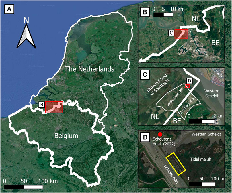
Figure 1. Overview of the location of the field experiment. (A) Area at the Dutch-Belgium border (B) Zoomed in on Western Scheldt at the Dutch-Belgium border, with Antwerp in the bottom right. (C) Zoomed in on the Hedwige-Prosperpolder, with the Western Scheldt in the top right and Drowned land of Saeftinghe in the top left (D) Zoomed in on the project site, with the yellow rectangle indicating the experimental site.
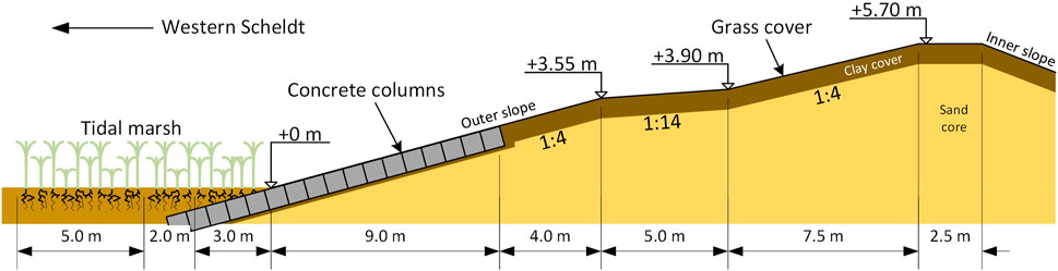
Figure 2. Dike cross-section with tidal marsh at the experimental site.
Schoutens et al. (2022) measured soil and vegetation characteristics at the tidal marsh 50 m North of the experimental site at end of January 2021 (Figure 1D). In this study we adopt their results, based on the assumption that in the proximity of this location, soil and vegetation conditions are also representative of our site. We confirmed this via visual observations of the vegetation density and state, and soil composition. Schoutens et al. (2022) measured large silt and clay fractions (72% and 17%, respectively), typical for tidal marshes. Organic matter content was measured at 20% and dry bulk density at 0.64 g cm−3. Shear strength at the surface was 13.01 kPa and at 10 cm depth was 31.75 kPa, which is likely affected by the many roots and rhizomes in the top layers. However, shear strength at the surface and at depth were determined with different devices. Brooks et al. (2023) show that comparing results between such devices should be done with caution.
The tidal marsh was homogeneously covered with Phragmites australis (common reed). Basal shoot diameter and shoot length were on average 0.46 and 204 cm, respectively. Flexural stiffness (resistance to bending) was 0.19 N m−2 and Young’s modulus (tensile strength) 6.7 × 10⁹ N m−2. The low flexural stiffness indicates that little force is required to significantly bend the reed stem. The high Young’s modulus (comparable to aluminium) indicates that the reed stems are able to withstand high strain loads (which increase as the bending angle increases) before breaking.
2.2 Flow flumes
The flow flumes were created using the Overflow Generator (OG), designed by Flanders Hydraulics for the Polder2C’s project (Vercruysse et al., 2023). The OG is designed to simulate continuous overflow of dike inner slopes over a 2 m wide section, for which it is placed on the outer slope facing the dike crest. For this study, the OG was placed on the dike inner slope instead, but also facing the crest (Figure 3). This way, the outflow water accelerated along the outer slope to the tidal marsh. Water was supplied to the OG using a pump installed at a nearby water source (here: the polder) and connected to the OG dissipation box using steel pipes. The pump used for the experiment had a maximum discharge capacity of 0.4 m3 s−1. The dissipation box spreads pump discharge equally over the width of the OG and dissipates most of the turbulence. A bridge element was used to cross the dike crest and link the OG with the flumes on the outer slope. Leakage was prevented as much as possible using EPDM (ethylene propylene diene monomer) sheets. From the bridge element to the dike toe, the flumes were constructed from concrete plywood planks supported by wooden piles (Supplementary Figures S1–S3). First, an approximately 10 cm deep incision was made in the grass cover in which the concrete plywood plank was placed. Then, the piles were hammered into the grass cover next to the planks and fixed with screws. At the concrete revetment, wooden supports (upside down T-shape) made from said piles were used and fixed with concrete screws (Supplementary Figure S4). The inside of these flumes (bottom and sides) was covered with blue plastic sheets to prevent grass cover erosion and minimise leakage. Sometimes, flumes were extended over the tidal marsh, see Section 2.3. Approximately 3 m behind the end of these flumes, a large trench was dug (1.5 × 1.5 m, cross-section) to drain the water exiting the flumes to the Western Scheldt.
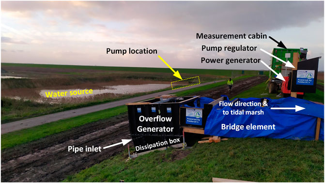
Figure 3. Overview of the Overflow Generator. Note: pump and pipes not yet installed.
2.3 Setup and monitoring
Three sections were tested in proximity of each other, see Figure 4. Close proximity prevents the need to move the OG, and minimises construction time and costs of the flumes. Also, it reduces the variation in soil and vegetation characteristics between the sections. The first two sections were tested for tidal marsh vegetation response and surface erodibility and the third for erodibility of deeper sediment layers. Section 1 was used to initially test the setup and then test the tidal marsh. Lessons learned from Section 1 were applied to Section 2. For Section 1 and Section 2 the flow flumes were extended 10–11 m onto the tidal marsh (Supplementary Figures S5, S6). The first 5 m of tidal marsh was mowed, of which the first 3 m covered with the blue plastic sheets to prevent erosion at the dike toe transition. Bed level measurements were done over a 5 m stretch, starting from 1 m after the end of the plastic sheet, see also Section 2.5. For Section 3, an approximately 1 m deep, 0.5 m wide trench was dug with an excavator (Supplementary Figure S7). All vegetation was mowed for easy access and because they were not of interest in this section. At the dike toe the tidal marsh was excavated to meet the bottom of the trench. The flume was narrowed to 0.5 m to achieve larger flow depths and consequently more soil area to erode. A scaled schematic of the setup is shown in Figure 4. The trench of Section 3 was directly connected to the drainage trench. Vegetation between flume exit and drainage trench was mowed to let the flow freely exit the flume.
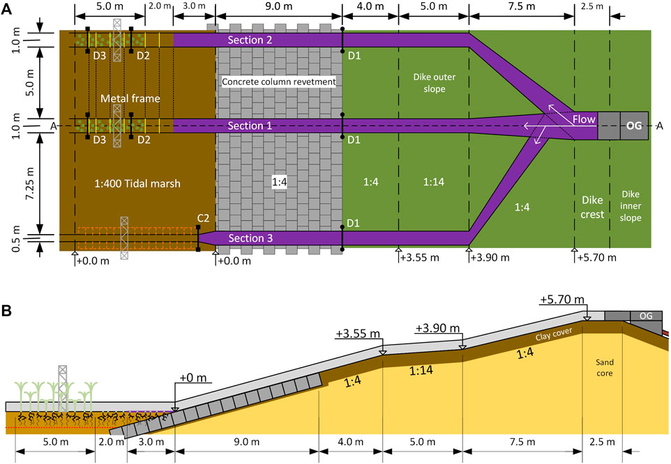
Figure 4. (A) Scaled schematic top view of the experiment setup. The Overflow Generator (OG) is indicated by the dark grey rectangles, the plastic sheets in purple and vegetation by the green circles (excl. vegetation outside of sections). The junction at the exit of the OG was not present during the experiment campaign, instead the flume panels were adjusted to connect with a section downstream directly. (B) Flumes are indicated by the light grey polygon. The red dotted line represents the bottom of the trench from Section 3. The tidal marsh has overgrown the concrete column revetment, which now extents below the tidal marsh to the dike outer toe.
Pump discharge was set by adjusting the pump frequency through a voltage regulator. An acoustic sensor on the inflow pipe measured the inflow discharge. On a local computer, the discharge was monitored and logged. Flow depth was measured manually with gauges at locations D1, D2, and D3 (Figure 4A). Secondly, pressure sensors were installed close to the bed at locations D2 and D3. A third pressure sensor at D2 was installed as barometer. Visual monitoring was done using a Go Pro Hero 7 Black at D2 and an Olympus TG-4 looking vertically downward from the metal frame.
2.4 Test series
The full experiment duration was 7 days, including (de) construction of the test setup and sections. The number of runs and the duration were limited by daylight and equipment availability. Therefore, each section was tested during a single day. Tests consisted of two to four runs of at least 30 min, see Table 1 for an overview. With each run, the discharge was increased until the maximum practical discharge is reached (0.34 m3 s−1 due to friction and head losses, which only occurred once for Section 2). For Section 1, the first two runs were done with a relatively low discharge to test the setup, investigate the initial response of the vegetation and capture the moment the tidal marsh erodes, if any. Based on the observations and results from Section 1, a higher initial discharge was chosen for Section 2. For Section 3, only two runs were possible with an effective maximum discharge of 0.24 m3 s−1, as above this discharge large volumes of water escaped the flume at the trench entry by overflowing trench edges due to the width constriction. From this point, discharge Q refers to the specific discharge used for a run.
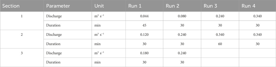
Table 1. Summary of test series.
The flow depth (d) is obtained from both manual measurements (depth gauges and probes) and the pressure sensors. Pressure sensor measurements are post-processed with the barometer measurements to account for atmospheric pressure fluctuations. Depth-averaged flow velocities (U) are calculated by dividing the effective discharge (Q) by the wetted area: U = Q/(W ⋅ d), where W = 1 m is the flume width. Froude number is calculated as: Fr = U/(g ⋅ d)0.5, where g = 9.81 m s−2 is the gravitational acceleration.
2.5 Bed level measurements
Bed levels are measured before and after each run using a probe with 0.5 cm accuracy. Bed level changes are calculated as the difference between subsequent corresponding measurements. Measurements for Section 1, Section 2 were taken in a 5 × 11 rectangular grid (Figure 5A) using slats with markings every 10 cm placed across the flume. For Section 3, the depth across the trench is measured every 0.5 m from the end of the protective plastic sheet (orange markings, Figure 5A) at three locations (left, centre and right, Figure 5B). The same technique as for Sections 1 and 2 is used. The width of the trench is obtained at the start from the distance between the left and right measurement.
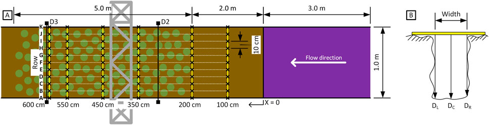
Figure 5. (A) Top view of the bed level measurement grid for Section 1 and Section 2. Each black cross represents one measurement point. The grey rectangle is the metal frame placed over the test section to mount a downwards facing camera. (B) Cross section example of the trench in Section 3 showing bed level and trench width measurement methods.
To determine if vegetation has a significant effect on the measured erosion, an one-factor ANalysis Of VAriance (ANOVA) test (Ståhle and Wold, 1989) is done for Section 1, Section 2. The bed level changes along the measured 5 m of a section are split into two groups: mowed (x = 1–3 m) and vegetated (x = 3–6 m). An ANOVA test compares the variance between and within the two groups to determine if the chosen independent variable (here: presence of vegetation) is a source of significant difference. The result of an ANOVA test is the F-value. Significance is accepted if F > Fcrit, where Fcrit is determined from the F-distribution, given a significance level (α, here: α = 0.05). Similarly, significance is accepted when the computed probability (p) that F > Fcrit is less than the given significance level.
2.6 Jet Erosion tests
Soil erosion resistance and erodibility are obtained from laboratory Jet Erosion Tests (Hanson and Cook, 2004) using the scour depth approach (Daly et al., 2013). A total of seven sample cores were collected 8 April 2021 using 15 cm high steel canisters with a 10 cm diameter. All cores were sampled from the tidal marsh surface layer except for SD-1, which was sampled from the bottom of the drainage trench (1.5 m below surface level), see Figure 6. First, a suitable undisturbed location within vegetation was found near the experimental site. Then, the canister with a metal cap was placed at the desired spot and pushed vertically into the soil (Figure 7A). Using a metal sledgehammer the canister was further hammered into the soil until the cap was mostly flat with the surface. The soil around the canister was removed to free it (Figure 7B). If roots were present at the underside of the canister, they were cut using a sharp toothed knife. The canister was then lifted free, the cap removed and excess material from the top 1–2 cm cut off (Figures 7C,D). For transport, canisters were closed on both sides with a cap, marked and sealed air-tight using tape. Prior to testing, sample immersion time was extended to 1 hour instead of the standard 10 min to simulate tidal flooding of the tidal marsh (as had happened the week prior to the experiment). Furthermore, a jet diameter of 12 mm was used because the size of the roots (rhizomes) present in the sample cores were of the same order as the standard jet diameter (6.35 mm). The initial hydraulic applied stress was set to 250 Pa to represent in-situ estimated stresses. Only the wet bulk density could be measured from the samples. Assuming soil properties are comparable to those in Schoutens et al. (2022), we can use their bulk dry density measurements to estimate the water content.
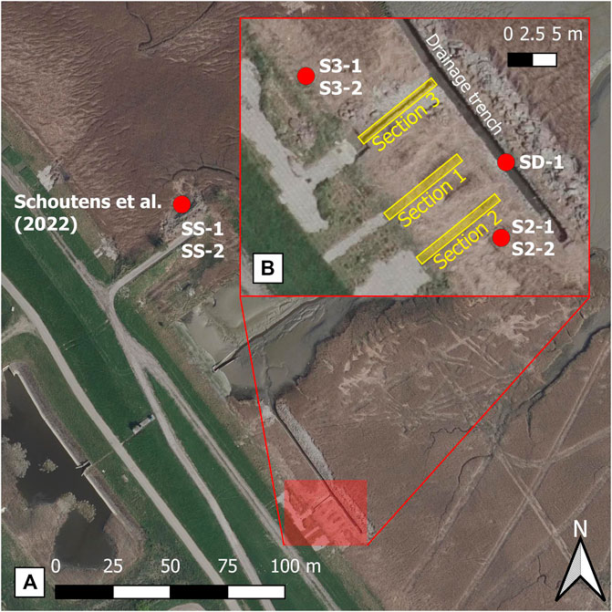
Figure 6. (A) Overview of soil and vegetation measurements by Schoutens et al. (2022) and JET soil sample locations (SS-1 and SS-2, taken at tidal marsh surface level). (B) Zoom in of JET sample locations around the experimental site. Samples S2-x, S3-x and SS-x were taken at tidal marsh surface level, while sample SD-1 was taken at the bottom of the trench (approximately 1.5 m below surface level).
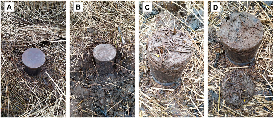
Figure 7. Sampling method for Jet Erosion Tests (A) Place canister at desired location (B) Hammer canister into ground and excavate around it (C) Extract sample and remove cap (D) Cut off top (1–2 cm) of the sample.
3 Results
3.1 Hydrodynamics
Outflow released from the OG accelerated down the slope of the dike, reaching supercritical flow conditions before the dike toe transition to the tidal marsh. For all runs, the abrupt change in slopes (steep to flat) resulted in hydraulic jumps, causing large energy losses. A hydraulic jump is the sudden transition of a flow from supercritical to subcritical conditions and is accompanied with much air entrainment and high shear stresses. For low discharges (0.044 and 0.080 m3 s−1) the jump occurred before the end of the plastic sheet protected area. For the higher discharges the jump either occurred on the mowed tidal marsh, or where the vegetation started. All hydraulic jumps for sections 1 and 2 were of the oscillating type (Fr = 2.4–4.5), or steady type (Fr = 4.5–9.0). For Section 3 all jumps occurred at the start of the section, where the flume width narrows to 0.5 m. Due to stem density differences and leaf litter, differences in flow patterns were visually observed. Where stem density was lower or where stems bent significantly, higher surface flow velocities were observed.
The measured flow depths and calculated depth-averaged flow velocities and Froude numbers are presented in Table 2. For Section 1 and Section 2 depth-averaged flow velocities ranged from 0.23 to 1.33 m s−1, and consequently Froude numbers varied between 0.23 and 0.84. Near-critical conditions (Fr ≈ 1) were not achieved in the test area of the flume, but only occurred at the flume exit where the reed behind the flume was mowed. Unexpectedly, measured flow depths generally decreased slightly for discharges exceeding 0.080 m3 s−1 while, commonly, flow depths will increase with increasing discharge (provided the bed roughness remains unchanged). Simultaneously, vegetation bent more at higher discharges (see Section 3.2). Therefore, it appears that an increased discharge (flow velocity) is accompanied with a reduction in vegetation induced drag, resulting in a decreased flow depth at higher discharges. This is discussed further in Section 4.1.
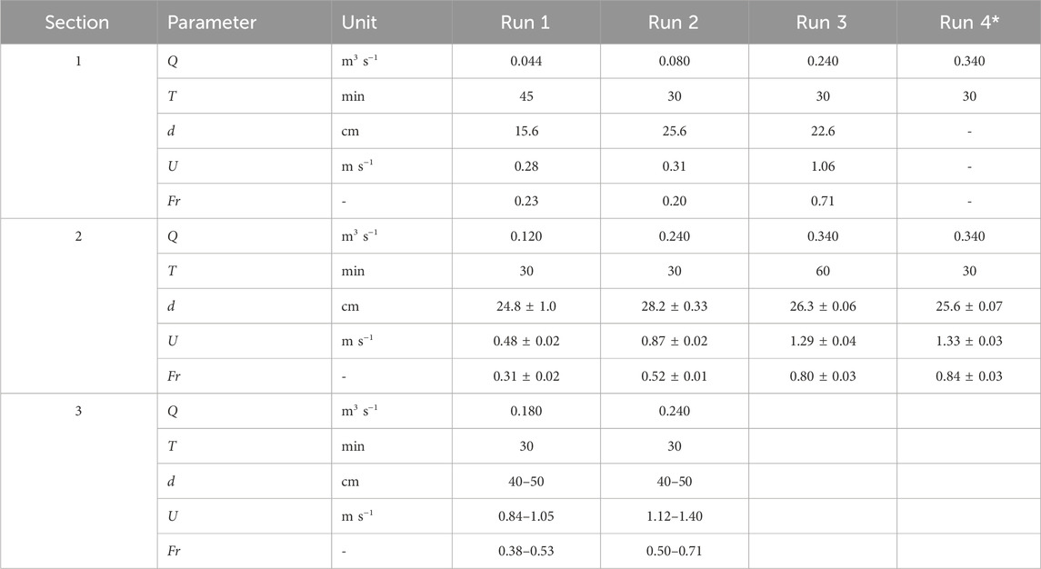
Table 2. Measured hydrodynamic parameters for each section and run, where Q is discharge, T is run duration, d is flow depth, U is depth-averaged flow velocity and Fr the Froude number. (*) Flow depth for Section 1 run 4 could not be accurately measured and thus omitted.
3.2 Vegetation response
Prior to testing Section 1 and Section 2, reed at the front of the section was already bent somewhat by wind or mowing. The rest of the reed stood (largely) upright, bended slightly by the wind. During the test runs the flow caused the reed to bend further, increasingly as the discharge increased. At low discharges (0.044 and 0.080 m3 s−1) bending was negligible, while at maximum discharge (0.34 m3 s−1) the reed bent as far as beneath the water surface. Stem response was not uniformly distributed along and across the flume. For Section 1, the reed at the right side (rows F-K) bent earlier, where also the stem density was visibly lower than at the left side (rows A-E). Even at the highest discharge, the tops of the stems (incl. foliage) remained visible (i.e., above the water surface). For Section 2, two stem patches near the end of the flume were visible during the first run, one at the right side (roughly x = 400–500 cm, rows H-K) and one somewhat further at the left side (at the lateral boundary of the test area and beyond). From run 2 onward, all vegetation in Section 2 bent to such an extent that the stems were entirely submerged. Once the discharge was stopped, stems were observed to recover quickly, with little to no broken stems. Within a few hours to a day the stems (almost) returned to their original position. The recovery ability of reed stems has also been observed (and measured) by Schoutens et al. (2022).
Leaf litter, accumulated in the sections between runs, built up in front of the shoots at low discharges. At higher discharges much of the leaf litter, though not all, would be transported and exit the flume. Even at maximum discharge some leaf litter would remain in the flume, captured between the stems. Where leaf litter remained, and between stems, eroded clumps of clay from the tidal marsh bed were found. These originated from within the test section or upstream from the test section (x = 0–100 cm). The presence of clay clumps indicate areas of low flow velocity.
3.3 Bed level changes
Measured bed level changes are shown in Figures 8, 9, and were of the order of centimetres. The eroded clumps of clay that were found between the stems and near the leaf litter deposits in Section 1 and Section 2 show up as sedimentation in the measurements. In Section 1 a maximum erosion of 5 cm was measured (after run 2). Erosion was generally larger at the right side of the flume (rows G-K), where also the highest flow velocities were observed (see Section 3.2). On the left side (rows A-D) mainly sedimentation occurred, where also vegetation appeared denser and showed less bending than on the right side. In Section 2 erosion was much more prominent, especially in the mowed region (x = 100–200 cm), although the observed maximum erosion was also 5 cm. A clear cause for the generally larger erosion in Section 2 was not found. We hypothesize that higher Froude numbers in this section lead to hydraulic jumps that generated higher bed shear stresses than in Section 1. Further down the flume (x = 300–600 cm) most erosion occurred in the centre (rows E-G), with only little erosion at the left side (rows A-D) and some sedimentation at the right side (rows H-K), again corresponding to locations where vegetation bent less or more. The observed erosion and sedimentation patterns suggest that vegetation might play an important role in determining the magnitude of erosion. However, ANOVA results for Section 1 and Section 2 respectively (F3.883 = 0.112, p = 0.73 and F3.877 = 3.613, p = 0.06), suggest that the presence of vegetation makes no significant difference. This discrepancy is discussed in Section 4.2.
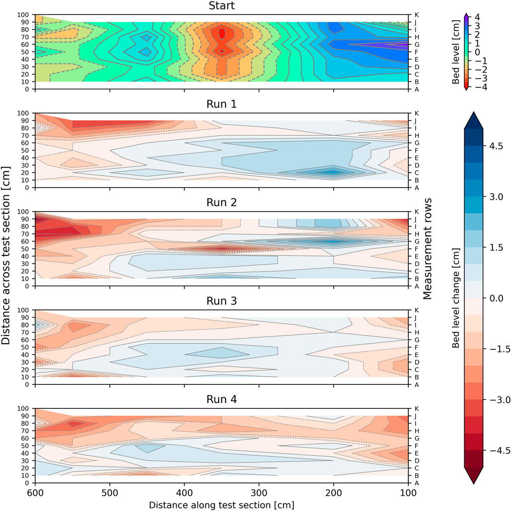
Figure 8. Plot of bed level changes for Section 1. Top figure shows the initial bed level relative to the mean. Subsequent plots down show the bed level changes for each run, with respect to the top figure. Positive means sedimentation, negative means erosion. Flow is from right to left.
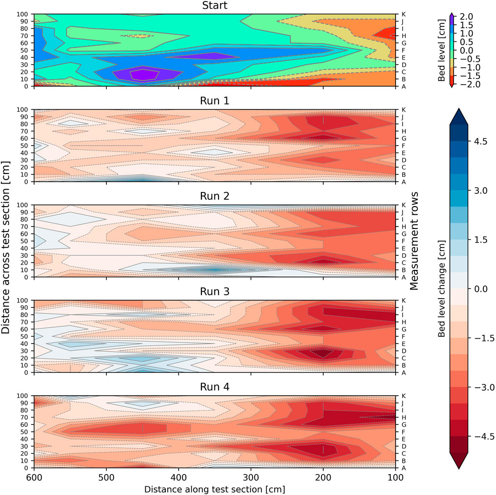
Figure 9. Plot of bed level changes for Section 2. Top figure shows the initial bed level relative to the mean. Subsequent plots down show the bed level changes for each run, with respect to the top figure. Positive means sedimentation, negative means erosion. Flow is from right to left.
Despite some sedimentation, the mean bed level in both Section 1 and Section 2 lowered with 0.71 and 1.81 cm, respectively (Figure 10). For both sections a period of initial erosion is observed for run 1 (in Section 1 for run 2 as well), after which subsequent runs did not increase the mean erosion. It is likely that mostly loose material and weak soil around vegetation stems erodes first. Afterwards, the mean bed level increased occasionally (Section 1, run 3; Section 2, run 2), or decreased marginally when either the discharge (section 1, run 4) or the run time (Section 2, run 4) were increased.
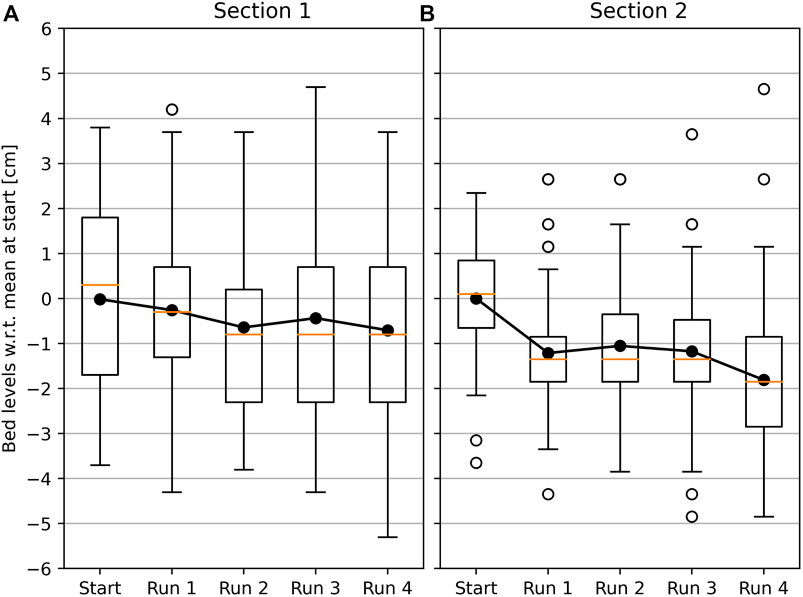
Figure 10. Boxplots of the measured bed levels for (A) Section 1 and (B) Section 2. The zero bed level is set to the mean bed level measured at the start. Mean bed level for each run is indicated by the connected black markers. Boxplots are presented with a median (orange line), an IQR (inter-quartile range) box, whiskers extending ±1.5 IQR and fliers as open dots.
Regarding Section 3, the part upstream of x = 4 m is excluded from the analysis due to measurement errors (x = 0–2 m) and lack of data (x = 2–4 m). In the remaining part of this section a maximum erosion of 4.5 cm was observed (Figure 11). The soil strength at 1.5 m depth is similar to the strength at the surface (based on the JET results, see Section 3.4) which explains the similar magnitude of the erosion in Section 3 when compared to Section 1 and Section 2. However, although not measured, trench walls eroded significantly and more of the root network got exposed (Supplementary Figure S8).
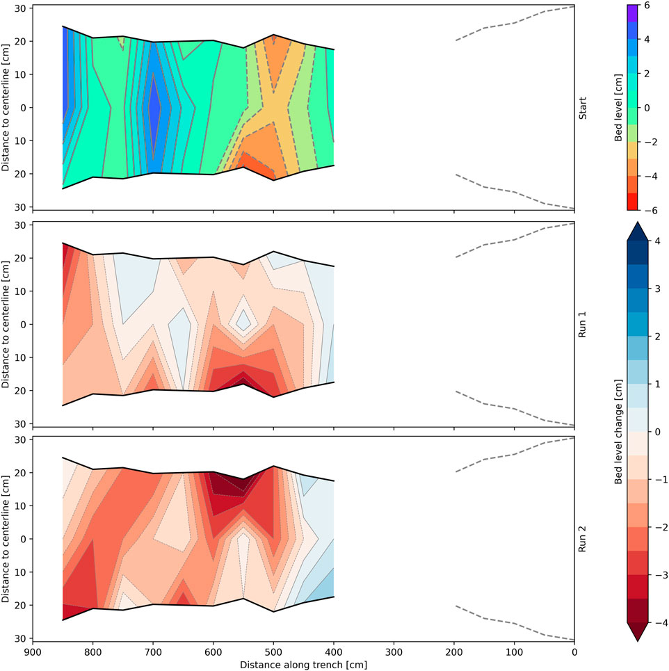
Figure 11. Plot of bed level changes for Section 3. Top figure shows the initial bed level relative to the mean. Subsequent plots down show the bed level changes for each run, with respect to the top figure. Positive means sedimentation, negative means erosion. Flow is from right to left.
3.4 Soil characteristics
The soil characteristics from the JET analysis (critical shear stress τc, erodibility kd, wet bulk density WD, estimated water content WC), and other JET parameters are given in Table 3. Out of the seven samples, two results (S2-1 and S3-1) are discarded due to questionable results and one sample (SS-2) could not be tested. Overall, from the remaining four results, the soil has a high resistance to erosion (τc = 85–140 Pa) and, unexpectedly, a high erodibility (kd = 27–45 cm3 N−1 s−1). For one sample (S2-2) a significantly lower erodibility of 6.5 cm3 N−1 s−1 was measured, which is attributed to the presence of a vertical rhizome in the sample at the location of the impinging jet. The rhizome dissipates most of the jet energy, reducing the energy available to erode the sediment. No clear cause for the high erodibility was found. More research is necessary as JET for rooted soils is scarce and its applicability for testing rooted soil may be questionable, as is discussed in Section 4.3.
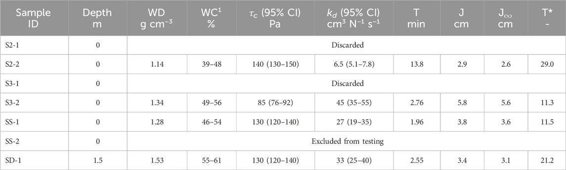
Table 3. Jet Erosion Test results: Wet bulk Density (WD), Water Content (WC), critical shear stress (τc), erodibility (kd), Confidence Interval (CI), test time (T), scour depth (J), theoretical scour depth at equilibrium (J∞) and dimensionless time (T*). 1The water content is estimated from the mean dry bulk density ± standard deviation measured by Schoutens et al. (2022).
Sample SD-1, taken at a depth of 1.5 m below the soil surface, has a slightly higher estimated water content (55%–61%) and wet bulk density (1.53 g cm−3) than the other samples, which were taken near the surface. Recall that immersion time was extended to 1 h for all samples, which could have affected the water content differences between the surface sample and sample SD-1.
All executed tests exceed the dimensionless time requirement (T* ≥10) defined by Stein et al. (1993). The dimensionless time T* is defined as the test duration (T) divided by a reference time Tr = J∞/(kdτc). When T* ≥10, Stein et al. (1993) found this warrants that the achieved scour depth in the test is within 95% of the equilibrium scour depth. Consequently, the obtained value for τc from our JET analysis is sufficiently reliable in that the actual value is unlikely to be lower than the measured one (see also Section 4.3).
4 Discussion
4.1 Vegetation effects on hydrodynamics
During the tests of Section 1 and Section 2, the tidal marsh vegetation bent more with increasing flow velocity. This behaviour is typical of flexible vegetation and is referred to as reconfiguration (Vogel, 1984). As the flexible vegetation bends more, the shape changes to become more streamlined with the flow. The cross-sectional flow area reduces, ultimately balancing the drag force with the restoring force (vegetation stiffness). In Vogel (1984) it was found that as the flow velocity increases, reconfiguration tends to a more linear relation between the drag force (FD) and the flow velocity (U), rather than the usual quadratic relation. To account for this effect, Vogel (1984) proposes to compute the drag force as FD ∝ U2+E, where E is a correction term referred to as Vogel’s exponent. Equations of this type also make use of a drag coefficient CD which, as studies have shown, varies significantly with stem density, stem Reynolds number and vegetation flexibility (Tanino and Nepf, 2008; Cheng, 2013; Chapman et al., 2015). However, most of such studies are done with (emergent) rigid bodies under steady uniform flows. Zhang et al. (2020) investigated the drag coefficient for immersed flexible artificial vegetation under steady non-uniform flow. They showed that flow entering dense vegetation first experiences an increase in drag, due to the blockage effect of the stems, and subsequently a decrease in drag due to their sheltering effect. The blockage effect relates to the stagnation and subsequent acceleration of the flow around a body causing, respectively, a pressure increment and a decrease of the wake pressure, together resulting in flow drag (Zdravkovich, 2003). The sheltering effect occurs when a body is located in the wake of an upstream body which causes a reduction in incident flow velocity and, consequently, a lower drag force (Raupach, 1992). In our experiments, all these effects were observed simultaneously. Firstly, higher discharges resulted in larger bending angles but no increase in flow depth. Thus, reconfiguration of the vegetation as flow velocity increased reduced its drag coefficient. Secondly, transversal stem density differences directed the flow to the lower density areas (blockage effect). Finally, stems downstream of densely vegetated patches bent less because of the reduced incident flow velocity (sheltering effect). For very large bending angles, when vegetation was fully immersed, reconfiguration appeared to be the dominant mechanism over blockage and sheltering. During a dike breach vegetation is expected to be permanently submerged, as opposed to this experiment, and the relative contributions of reconfiguration, blocking and sheltering on the hydrodynamics will be different. In this situation the increased submergence enhances the reconfiguration effect which, involving less exposure of the vegetation to the flow, reduces the blockage and sheltering effect.
For submerged vegetation, typically referred to as a meadow or canopy, the corresponding drag depends mainly on the depth of submergence, stem density and bending angle (Nepf, 2011; 2012a; b). If this drag dominates the bed induced drag, a shear layer will develop near the top of the canopy. This implies an inflection point near the canopy where the Reynolds stresses are largest (Zhang et al., 2023), separating the velocity profiles for the vegetation layer and free flow layer, respectively (Wang et al., 2015; 2023). The velocity profile in the free flow layer is logarithmic, while in the vegetation layer turbulence and dispersion effects associated with the stems result in a different velocity distribution. Consequently, flow velocities in the free flow layer can be significantly larger than in the layer covered by vegetation and thus convey a larger fraction of the total discharge, which also reduces the shear stress acting directly on the soil particles. In this study, the vegetation was emerged for low discharges but eventually submerged for high discharges. Although not investigated in detail, the observations confirmed that in submerged cases two flow layers were present. However, the corresponding velocity profiles and bed shear stresses that actually cause the pick-up of bed material were not measured. Assessing the soil stability for near-critical flow conditions and high flow velocities would also require the soil and vegetation properties. More experiments with high-velocity conditions, also considering different combinations of soil composition and vegetation type, are therefore needed to derive generic process based erosion models.
4.2 Interpretation of erosion results
The observed erosion in this study was minimal (order centimetres, maximum 5 cm), for all sections, after a maximum of 2–2.5 h of cumulative exposure to a step-by-step increased hydrodynamic forcing (increased flow velocity). Moreover, the bulk of the erosion was measured where vegetation was either mowed or had relatively low stem density, highlighting the importance of vegetation for soil stability under these conditions. However, these results are difficult to extrapolate to other tidal marshes as soil composition and vegetation type can significantly vary within a marsh and between tidal marshes. Studies of tidal marsh erosion at high flow velocities (
Stoorvogel et al. (2024) measured erosion of a restored and a natural tidal marsh (mowed/clipped) at Lippenbroek (Belgium) under flow velocities up to 4.3 ms−1 for 3 hours. Erosion of both the restored and natural tidal marsh was measured to be of the order of centimetres, again a similar magnitude as in our study. Marin-Diaz et al. (2022) measured up to 2 cm of erosion after 3 h of exposure to flow velocities of 2.3 m−1 for different silty tidal marshes. Based on the combined outcome of Marin-Diaz et al. (2022), Schoutens et al. (2022), Stoorvogel et al. (2024) and our study, we argue that vegetated tidal marshes are very stable, at least for the type of marshes considered in these studies. This confirms the important benefits of tidal marshes in case of a dike breach, where the effectiveness of a tidal marsh is highly dependent on the soil stability.
Tidal marshes develop over many years or even decades. As they grow, the early sediment layers consolidate due to the load of the layers above, which increases the bulk density. When vegetation grows, a rooted layer is formed at the top. In tidal marsh soil columns at least two main layers can therefore be distinguished: a rooted top layer and a deeper layer. Both the consolidation of the deeper layer and the vegetation at the top layer enhance the soil stability (Ford et al., 2016; Bernik et al., 2018; Chen et al., 2019). The stabilizing effect of vegetation is more prominent in coarser (sand) soils than in fine (silt/clay) soils (Lo et al., 2017). The latter would explain why in the JET results for our silty marsh no clear difference was found between the erosion resistance and erodibility at the surface (many roots) and at 1.5 m depth (few roots). Moreover, the bulk density at 1.5 m depth was only slightly higher than at the surface, indicating that the degree of consolidation hardly varies over the depth for this tidal marsh. There was one exception though (surface sample S2-2) where the erodibility was much lower, likely due to a protruding rhizome. The size of the jet and rhizome were similar, meaning the jet impacted the rhizome predominantly instead of the soil. Thus, these roots can significantly reduce erodibility of a tidal marsh. However, a bigger jet may overcome this issue. Nonetheless, it is conjectured that for silty tidal marshes the roots affect the erodibility more than the erosion resistance under JET-like hydrodynamic forcing. As this is based on only a very small sample size, further research is needed to confirm this.
The linear excess stress equation is often used to estimate the erosion of soils, and is formulated as E = kd (τb − τc), where E is the erosion rate in m s−1 and τb bed shear stress in Pa. The erosion measurements in this study (JET and in-situ) reveal that such an equation must be used with care, considering all of its input parameters. As example, the bed shear stress can be estimated as τb = gC−2ρU2, where ρ is the water density and C is the Chézy parameter which in this case - based on methods by Baptist et al. (2007) and Luhar and Nepf (2013) and using parameter values from Van Velzen et al. (2003) and Schoutens et al. (2022)—has a value between 5 and 11 m1/2 s−1. For cases where U < 0.5 m−1 (Section 1, runs 1–2; Section 2, run 1) this results in a bed shear stress (τb) that is smaller than the lowest measured critical bed shear stress (τc < 85 Pa, see Table 2). Consequently, no erosion should occur which appears true for Section 1 (if it is assumed that bed level changes are only due to transport of leaf litter and loose material), but not so for Section 2 where much erosion was measured after run 1. For cases where U > 0.5 m s−1, the estimated τb can exceed the measured τc (85, 130, and 140 Pa) by up to two orders of magnitude. Using the linear excess stress equation then leads to erosion estimates that are up to two orders of magnitude larger than the measured (maximum) erosion. This discrepancy is explained by the fact that the estimated Chézy-values model the vegetation drag experienced by the flow, rather than the shear stress experienced by the soil particles, ignoring the typical velocity profile and turbulence characteristics in the canopy that affect the latter (Section 4.1). Using this approach, the effective bed shear stress is likely overestimated and so is the predicted erosion, in particular for high flow velocities when sheltering by vegetation is more pronounced. Furthermore, methods to determine kd and τc, such as JET analysis, should also account for these in-situ hydrodynamics. This is discussed in more detail in Section 4.3. In conclusion, proper use of the linear excess stress equation for tidal marshes requires input parameter values that take both above- and below ground biomass into account to avoid overestimation of tidal marsh erosion rates.
4.3 Validity of JET for measuring soil erosion resistance and erodibility
Estimating the soil erosion resistance and erodibility from general soil characteristics remains difficult, especially for cohesive soils, and no universally accepted methodology exists today (Knapen et al., 2007). The best practice still is to acquire these properties from laboratory or in-situ tests. One of these methods is the Jet Erosion Test, which is used in this study. This method relies on the assumptions that the impinging jet is unconfined, that the jet acts on a smooth, flat bed and that erosion is linearly proportional to the excess shear stress. These starting points bear some limitations, however. Firstly, assuming an unconfined jet leads to underestimation of the maximum applied shear stress by a factor of 2.4 or more (Ghaneeizad et al., 2015). Secondly, during the scour process a hole develops which alters the flow regime (Mercier et al., 2012), thereby changing the shear stress magnitude and - distribution along the jet centre line, as compared to a flat bed. Thirdly, the maximum shear stress on a rough bed can be 2.5–5 times larger than on a smooth bed (Rajaratnam and Mazurek, 2005). Lastly, in Zhu et al. (2001) it is shown that power law stress equations generally provide better fits to JET test data than linear equations. Nevertheless, they recommend using the latter in case of high shear stresses and longer slopes (referring to the slope length in their experiment). These findings are not yet implemented in the JET standard, however, and the interpretation of its results should therefore consider the implications of the aforementioned assumptions.
Comparing our in-situ observations with the results from the JET analysis indicates that τc is underestimated while kd is overestimated, as the predicted erosion rates (based on JET) generally exceed those observed in the field. Furthermore, none of the JET results is consistent with τc − kd relationships found in literature, see for instance Karamigolbaghi et al. (2017). The relatively low τc that is obtained from JET directly relates to the shortcomings mentioned before. Regarding kd, a lower erodibility from flume tests as compared to JET tests has also been reported by McNichol et al. (2017), but this was not statistically validated. We hypothesise two main causes for overestimating the value of kd when using JET. Firstly, the impinging flow in JET is perpendicular to the sample while the in-situ flow velocity is mainly parallel to the bed. This difference is avoided using HET (Hole Erosion Test, Wan and Fell (2004)), where a hole is drilled through a sample which is then exposed to flow, in a way similar to piping erosion. HET analysis consistently produces lower kd and higher τc values (Regazzoni et al., 2008; Wahl, 2010; Regazzoni and Marot, 2013). Secondly, in flume tests the presence of aboveground biomass reduces the transport capacity of the flow due to sheltering by the vegetation canopy, an effect that is not accounted for in JET nor in HET.
Concluding, although JET remains the most popular method due to its applicability to a wide range of soils and generally accepted use, it appears to overestimate the erodibility and underestimate the erosion resistance of tidal marshes. Other methods (such as HET) might be more suited for this specific situation. In any case, the valid use of these erosion parameters in (linear) excess stress equations relies on tests accounting for the effect of aboveground biomass.
4.4 Tidal marshes under dike breach conditions
In this study we tested an in-situ tidal marsh under dike breach conditions (i.e., high flow velocities). With the experimental setup we achieved flow depths of 0.2–0.25 m, and a maximum flow velocity of 1.3 ms−1, while the tidal marsh was exposed to a cumulative 2–2.5 h of hydrodynamic forcing. During a storm surge water depths on a tidal marsh can amount up to 2.0–2.5 m, which then results in flow velocities of up to 4–5 m s−1 during a dike breach, an event that can typically last up to 4 h during peak storm surges. Therefore, in our experiment, the overall exposure of the tidal marsh to hydrodynamic forcing was comparatively mild, both in terms of flow velocities and duration.
Nonetheless, the experiment revealed that higher flow velocities do not always lead to increased erosion which, being of the order of centimetres only, remained limited under these conditions. Other studies (Marin-Diaz et al., 2022; Schoutens et al., 2022; Stoorvogel et al., 2024) tested tidal marshes for a duration of 3–12 h and measured similar erosion rates, of the order of millimetres to centimetres. These results indicate that, under dike breach conditions, only limited erosion of a tidal marsh will take place. The precise rate and magnitude of this erosion remains difficult to predict for these conditions, however.
This study re-emphasises that mature silty tidal marshes are strong and likely to survive a dike breach, considering that erosion is of the order of only centimetres while tidal marshes can be 1–2 m thick. If tidal marsh levels hardly change during a breach, erosion of the dike will result in a vertical or near-vertical drop in the local bed elevation, referred to as head-cut (Zhu et al., 2008). For dike breach modelling, a constant tidal marsh level is therefore a viable assumption, provided that the high erosion resistance and low erodibility of the tidal marsh are confirmed, leaving head-cut failure as the primary erosion mechanism.
5 Conclusion
In order to warrant flood defences future proof, in the light of climate change, researchers and engineers have an increased interest in Nature based Solutions (NbS). As such, tidal marshes have an intrinsic ecological value while they also reduce the failure probability and breach erosion rates of adjacent dikes. The latter highly depends on the stability of the tidal marsh during dike breach conditions, requiring insight in its erosion resistance and erodibility. This study is one of the first that specifically aims at a better understanding of these properties under high flow velocities,
Data availability statement
The datasets presented in this study can be found in online repositories. The names of the repository/repositories and accession number(s) can be found below: 10.4121/8dfca93b-ffff-4e1d-b2e3-fe980716c658.
Author contributions
MvB: Conceptualization, Data curation, Formal Analysis, Investigation, Methodology, Validation, Visualization, Writing–original draft, Writing–review and editing. SR: Conceptualization, Methodology, Writing–review and editing. SA: Conceptualization, Funding acquisition, Writing–review and editing. RL: Writing–review and editing.
Funding
The author(s) declare financial support was received for the research, authorship, and/or publication of this article. This study is part of the project: The Hedwige-Prosper Polder as a future-oriented experiment in managed realignment: integrating saltmarshes in water safety (Project number: 17589) of the research programme Living Labs in the Dutch Delta which is (partly) financed by the Dutch Research Council (NWO).
Acknowledgments
We would like to thank Patrik Peeters and the on-site team from Flanders Hydraulics for helping with logistics, materials, equipment and building the setup. A special thanks to Jord Smid, who accompanied me for the entire week. We also thank the members of Waterlab at Delft University of Technology for helping with the design of the flumes, and preparation and installation of the equipment. Thank you Geert Vanwesenbeeck from Jan de Nul N.V. for providing machinery and its logistics. A thank you to Ken Schoutens, Marte Stoorvogel and Kim van den Hoven for their insights. Gratitude goes to Maxime Boucher from GeophyConsult for supplying JET equipment, advice on test procedure, performing the tests and assisting in interpretation. Lastly, a big thank you to Peter Herman for bringing a plethora of ecological and biological perspectives. Peter is now retired but was an active member of the research team that initiated and conducted this study.
Conflict of interest
The authors declare that the research was conducted in the absence of any commercial or financial relationships that could be construed as a potential conflict of interest.
Publisher’s note
All claims expressed in this article are solely those of the authors and do not necessarily represent those of their affiliated organizations, or those of the publisher, the editors and the reviewers. Any product that may be evaluated in this article, or claim that may be made by its manufacturer, is not guaranteed or endorsed by the publisher.
Supplementary material
The Supplementary Material for this article can be found online at: https://www.frontiersin.org/articles/10.3389/fenvs.2024.1385610/full#supplementary-material
References
Almar, R., Ranasinghe, R., Bergsma, E. W. J., Diaz, H., Melet, A., Papa, F., et al. (2021). A global analysis of extreme coastal water levels with implications for potential coastal overtopping. Nat. Commun. 12, 3775. doi:10.1038/s41467-021-24008-9
Baptist, M., Babovic, V., Rodríguez Uthurburu, J., Keijzer, M., Uittenbogaard, R., Mynett, A., et al. (2007). On inducing equations for vegetation resistance. J. Hydraulic Res. 45, 435–450. doi:10.1080/00221686.2007.9521778
Barbier, E. B., Hacker, S. D., Kennedy, C., Koch, E. W., Stier, A. C., and Silliman, B. R. (2011). The value of estuarine and coastal ecosystem services. Ecol. Monogr. 81, 169–193. doi:10.1890/10-1510.1
Bax, V., van de Lageweg, W. I., Terpstra, T., Buijs, J.-M., de Reus, K., de Groot, F., et al. (2023). The impact of coastal realignment on the availability of ecosystem services: gains, losses and trade-offs from a local community perspective. J. Environ. Manag. 345, 118675. doi:10.1016/j.jenvman.2023.118675
Bernik, B., Pardue, J., and Blum, M. (2018). Soil erodibility differs according to heritable trait variation and nutrient-induced plasticity in the salt marsh engineer Spartina alterniflora. Mar. Ecol. Prog. Ser. 601, 1–14. doi:10.3354/meps12689
Billah, M. M., Bhuiyan, M. K. A., Islam, M. A., Das, J., and Hoque, A. R. (2022). Salt marsh restoration: an overview of techniques and success indicators. Environ. Sci. Pollut. Res. 29, 15347–15363. doi:10.1007/s11356-021-18305-5
Bouma, T. J., Vries, M. B. D., Low, E., Kusters, L., Herman, P. M. J., Tánczos, I. C., et al. (2005). Flow hydrodynamics on a mudflat and in salt marsh vegetation: identifying general relationships for habitat characterisations. Hydrobiologia 540, 259–274. doi:10.1007/s10750-004-7149-0
Brooks, H., Moeller, I., Spencer, T., and Royse, K. (2023). Shear strength and erosion resistance of salt marsh substrates: which method to use? Estuar. Coast. Shelf Sci. 292, 108452. doi:10.1016/j.ecss.2023.108452
Chapman, J. A., Wilson, B. N., and Gulliver, J. S. (2015). Drag force parameters of rigid and flexible vegetal elements. Water Resour. Res. 51, 3292–3302. doi:10.1002/2014WR015436
Chen, Y., Thompson, C., and Collins, M. (2019). Controls on creek margin stability by the root systems of saltmarsh vegetation, Beaulieu Estuary, Southern England. Anthr. Coasts 2, 21–38. doi:10.1139/anc-2018-0005
Cheng, N.-S. (2013). Calculation of drag coefficient for arrays of emergent circular cylinders with pseudofluid model. J. Hydraulic Eng. 139, 602–611. doi:10.1061/(ASCE)HY.1943-7900.0000722
Daly, E. R., Fox, G. A., Miller, R. B., and Al-Madhhachi, A.-S. T. (2013). A scour depth approach for deriving erodibility parameters from jet erosion tests. Trans. ASABE, 1343–1351. doi:10.13031/trans.56.10350
Davidson, N. C. (2014). How much wetland has the world lost? Long-term and recent trends in global wetland area. Mar. Freshw. Res. 65, 934. doi:10.1071/MF14173
De Battisti, D., Fowler, M. S., Jenkins, S. R., Skov, M. W., Rossi, M., Bouma, T. J., et al. (2019). Intraspecific root trait variability along environmental gradients affects salt marsh resistance to lateral erosion. Front. Ecol. Evol. 7. doi:10.3389/fevo.2019.00150
Fang, J., Nicholls, R. J., Brown, S., Lincke, D., Hinkel, J., Vafeidis, A. T., et al. (2022). Benefits of subsidence control for coastal flooding in China. Nat. Commun. 13, 6946. doi:10.1038/s41467-022-34525-w
Ford, H., Garbutt, A., Ladd, C., Malarkey, J., and Skov, M. W. (2016). Soil stabilization linked to plant diversity and environmental context in coastal wetlands. J. Veg. Sci. 27, 259–268. doi:10.1111/jvs.12367
Gedan, K. B., Silliman, B., and Bertness, M. (2009). Centuries of human-driven change in salt marsh ecosystems. Annu. Rev. Mar. Sci. 1, 117–141. doi:10.1146/annurev.marine.010908.163930
Ghaneeizad, S. M., Karamigolbaghi, M., Atkinson, J. F., and Bennett, S. J. (2015). “Hydrodynamics of confined impinging jets and the assessment of soil erodibility,” in World environmental and water resources congress 2015 (Reston, VA: American Society of Civil Engineers), 1742–1751. doi:10.1061/9780784479162.170
Hanson, G. J., and Cook, K. (2004). Apparatus, test procedures, and analytical methods to measure soil erodibility in situ. Appl. Eng. Agric. 20. doi:10.13031/2013.16492
Horton, B. P., Shennan, I., Bradley, S. L., Cahill, N., Kirwan, M., Kopp, R. E., et al. (2018). Predicting marsh vulnerability to sea-level rise using Holocene relative sea-level data. Nat. Commun. 9, 2687. doi:10.1038/s41467-018-05080-0
Johnston, J., Cassalho, F., Miesse, T., and Ferreira, C. M. (2021). Projecting the effects of land subsidence and sea level rise on storm surge flooding in Coastal North Carolina. Sci. Rep. 11, 21679. doi:10.1038/s41598-021-01096-7
Karamigolbaghi, M., Ghaneeizad, S. M., Atkinson, J. F., Bennett, S. J., and Wells, R. R. (2017). Critical assessment of jet erosion test methodologies for cohesive soil and sediment. Geomorphology 295, 529–536. doi:10.1016/j.geomorph.2017.08.005
Kirezci, E., Young, I. R., Ranasinghe, R., Muis, S., Nicholls, R. J., Lincke, D., et al. (2020). Projections of global-scale extreme sea levels and resulting episodic coastal flooding over the 21st Century. Sci. Rep. 10, 11629. doi:10.1038/s41598-020-67736-6
Kirwan, M. L., Temmerman, S., Skeehan, E. E., Guntenspergen, G. R., and Fagherazzi, S. (2016). Overestimation of marsh vulnerability to sea level rise. Nat. Clim. Change 6, 253–260. doi:10.1038/nclimate2909
Knapen, A., Poesen, J., Govers, G., Gyssels, G., and Nachtergaele, J. (2007). Resistance of soils to concentrated flow erosion: a review. Earth-Science Rev. 80, 75–109. doi:10.1016/j.earscirev.2006.08.001
Liu, M., Luo, Y., Qiao, C., Wang, Z., Ma, H., and Sun, D. (2023). The hydraulic and boundary characteristics of a dike breach based on cluster analysis. Water 15, 2908. doi:10.3390/w15162908
Lo, V., Bouma, T., van Belzen, J., Van Colen, C., and Airoldi, L. (2017). Interactive effects of vegetation and sediment properties on erosion of salt marshes in the Northern Adriatic Sea. Mar. Environ. Res. 131, 32–42. doi:10.1016/j.marenvres.2017.09.006
Luhar, M., and Nepf, H. M. (2013). From the blade scale to the reach scale: a characterization of aquatic vegetative drag. Adv. Water Resour. 51, 305–316. doi:10.1016/j.advwatres.2012.02.002
MacManus, K., Balk, D., Engin, H., McGranahan, G., and Inman, R. (2021). Estimating population and urban areas at risk of coastal hazards, 1990–2015: how data choices matter. Earth Syst. Sci. Data 13, 5747–5801. doi:10.5194/essd-13-5747-2021
Marin-Diaz, B., Govers, L. L., van der Wal, D., Olff, H., and Bouma, T. J. (2022). The importance of marshes providing soil stabilization to resist fast-flow erosion in case of a dike breach. Ecol. Appl. 32, e2622. doi:10.1002/eap.2622
McGranahan, G., Balk, D., and Anderson, B. (2007). The rising tide: assessing the risks of climate change and human settlements in low elevation coastal zones. Environ. Urbanization 19, 17–37. doi:10.1177/0956247807076960
McNichol, B., Kassa, K., Fox, G., Miller, R., and Guertault, L. (2017). Erodibility parameters derived from jet and flume erosion tests on root-permeated soils. J. Contemp. Water Res. Educ. 160, 119–131. doi:10.1111/j.1936-704X.2017.03244.x
Mercier, F., Bonelli, S., Anselmet, F., Pinettes, P., Courivaud, J. R., and Fry, J. J. (2012). On the numerical modelling of the jet erosion test. in 6th international conference on scour and erosion (France: Paris), 600–608.
Mitchell, M., Herman, J., Bilkovic, D. M., and Hershner, C. (2017). Marsh persistence under sea-level rise is controlled by multiple, geologically variable stressors. Ecosyst. Health Sustain. 3. doi:10.1080/20964129.2017.1396009
Möller, I., Kudella, M., Rupprecht, F., Spencer, T., Paul, M., van Wesenbeeck, B. K., et al. (2014). Wave attenuation over coastal salt marshes under storm surge conditions. Nat. Geosci. 7, 727–731. doi:10.1038/ngeo2251
Möller, I., Spencer, T., French, J., Leggett, D., and Dixon, M. (1999). Wave transformation over salt marshes: a field and numerical modelling study from North norfolk, england. Estuar. Coast. Shelf Sci. 49, 411–426. doi:10.1006/ecss.1999.0509
Morris, J. T., Barber, D. C., Callaway, J. C., Chambers, R., Hagen, S. C., Hopkinson, C. S., et al. (2016). Contributions of organic and inorganic matter to sediment volume and accretion in tidal wetlands at steady state. Earth’s Future 4, 110–121. doi:10.1002/2015EF000334
Nepf, H. (2011). “Flow over and through biota,” in Treatise on estuarine and coastal science (Elsevier), 267–288. doi:10.1016/B978-0-12-374711-2.00213-8
Nepf, H. M. (2012a). Flow and transport in regions with aquatic vegetation. Annu. Rev. Fluid Mech. 44, 123–142. doi:10.1146/annurev-fluid-120710-101048
Nepf, H. M. (2012b). Hydrodynamics of vegetated channels. J. Hydraulic Res. 50, 262–279. doi:10.1080/00221686.2012.696559
Neumann, B., Vafeidis, A. T., Zimmermann, J., and Nicholls, R. J. (2015). Future coastal population growth and exposure to sea-level rise and coastal flooding - a global assessment. PLOS ONE 10, e0118571. doi:10.1371/journal.pone.0118571
Nicholls, R. J., Lincke, D., Hinkel, J., Brown, S., Vafeidis, A. T., Meyssignac, B., et al. (2021). A global analysis of subsidence, relative sea-level change and coastal flood exposure. Nat. Clim. Change 11, 338–342. doi:10.1038/s41558-021-00993-z
Peeters, P., Van Hoestenberghe, T., Vincke, L., and Visser, P. (2011). “SWOT analysis of breach models for common dike failure mechanisms,” in Proceedings of the 34th IAHR world congress (Brisbane: Oikos), 3936–3943.
Pontee, N. (2013). Defining coastal squeeze: a discussion. Ocean Coast. Manag. 84, 204–207. doi:10.1016/j.ocecoaman.2013.07.010
Rajaratnam, N., and Mazurek, K. (2005). Impingement of circular turbulent jets on rough boundaries. J. Hydraulic Res. 43, 689–695. doi:10.1080/00221680509500388
Raupach, M. R. (1992). Drag and drag partition on rough surfaces. Boundary-Layer Meteorol. 60, 375–395. doi:10.1007/BF00155203
Regazzoni, P., Marot, D., Courivaud, J., Hanson, G., and Wahl, T. (2008). “Soil erodibility: a comparison between the jet erosion test and the hole erosion test,” in Inaugural international Conference of the engineering mechanics institute (Minneapolis, USA: ASCE).
Regazzoni, P.-L., and Marot, D. (2013). A comparative analysis of interface erosion tests. Nat. Hazards 67, 937–950. doi:10.1007/s11069-013-0620-3
Saintilan, N., Kovalenko, K. E., Guntenspergen, G., Rogers, K., Lynch, J. C., Cahoon, D. R., et al. (2022). Constraints on the adjustment of tidal marshes to accelerating sea level rise. Science 377, 523–527. doi:10.1126/science.abo7872
Schoutens, K., Stoorvogel, M., van den Berg, M., van den Hoven, K., Bouma, T. J., Aarninkhof, S., et al. (2022). Stability of a tidal marsh under very high flow velocities and implications for nature-based flood defense. Front. Mar. Sci. 9. doi:10.3389/fmars.2022.920480
Scott, D. B., Frail-Gauthier, J., and Mudie, P. J. (2014) Coastal wetlands of the world. Cambridge University Press. doi:10.1017/CBO9781107296916
Shirzaei, M., Freymueller, J., Törnqvist, T. E., Galloway, D. L., Dura, T., and Minderhoud, P. S. J. (2020). Measuring, modelling and projecting coastal land subsidence. Nat. Rev. Earth Environ. 2, 40–58. doi:10.1038/s43017-020-00115-x
Ståhle, L., and Wold, S. (1989). Analysis of variance (ANOVA). Chemom. Intelligent Laboratory Syst. 6, 259–272. doi:10.1016/0169-7439(89)80095-4
Stein, O. R., Julien, P. Y., and Alonso, C. V. (1993). Mechanics of jet scour downstream of a headcut. J. Hydraulic Res. 31, 723–738. doi:10.1080/00221689309498814
Stoorvogel, M., Temmerman, S., Oosterlee, L., Schoutens, K., Maris, T., Van de Koppel, J., et al. (2024) Nature-based shoreline protection in newly formed tidal marshes is controlled by tidal inundation and sedimentation rate.
Stralberg, D., Brennan, M., Callaway, J. C., Wood, J. K., Schile, L. M., Jongsomjit, D., et al. (2011). Evaluating tidal marsh sustainability in the face of sea-level rise: a hybrid modeling approach applied to San Francisco bay. PLoS ONE 6, e27388. doi:10.1371/journal.pone.0027388
Taherkhani, M., Vitousek, S., Barnard, P. L., Frazer, N., Anderson, T. R., and Fletcher, C. H. (2020). Sea-level rise exponentially increases coastal flood frequency. Sci. Rep. 10, 6466. doi:10.1038/s41598-020-62188-4
Tanino, Y., and Nepf, H. M. (2008). Laboratory investigation of mean drag in a random array of rigid, emergent cylinders. J. Hydraulic Eng. 134, 34–41. doi:10.1061/(ASCE)0733-9429(2008)134:1(34)
Tay, C., Lindsey, E. O., Chin, S. T., McCaughey, J. W., Bekaert, D., Nguyen, M., et al. (2022). Sea-level rise from land subsidence in major coastal cities. Nat. Sustain. 5, 1049–1057. doi:10.1038/s41893-022-00947-z
Temmerman, S., Horstman, E. M., Krauss, K. W., Mullarney, J. C., Pelckmans, I., and Schoutens, K. (2023). Marshes and mangroves as nature-based coastal storm buffers. Annu. Rev. Mar. Sci. 15, 95–118. doi:10.1146/annurev-marine-040422-092951
Temmerman, S., Meire, P., Bouma, T. J., Herman, P. M. J., Ysebaert, T., and De Vriend, H. J. (2013). Ecosystem-based coastal defence in the face of global change. Nature 504, 79–83. doi:10.1038/nature12859
van den Hoven, K., van Belzen, J., Kleinhans, M. G., Schot, D. M., Merry, J., van Loon-Steensma, J. M., et al. (2023). How natural foreshores offer flood protection during dike breaches: an explorative flume study. Estuar. Coast. Shelf Sci. 294, 108560. doi:10.1016/j.ecss.2023.108560
Van Velzen, E., Jesse, P., Cornelissen, P., and Coops, H. (2003). Stromingsweerstand vegetatie in uiterwaarden. Ministerie van Verkeer en Waterstaat, Arnhem: Arnhem. Tech. rep.
Vercruysse, J., Depreieter, D., López Castaño, S., Verelst, K., and Peeters, P. (2023) Design and application of an overflow generator. Antwerp: Flanders Hydraulics. Tech. rep.
Vitousek, S., Barnard, P. L., Fletcher, C. H., Frazer, N., Erikson, L., and Storlazzi, C. D. (2017). Doubling of coastal flooding frequency within decades due to sea-level rise. Sci. Rep. 7, 1399. doi:10.1038/s41598-017-01362-7
Vogel, S. (1984). Drag and flexibility in sessile organisms. Am. Zoologist 24, 37–44. doi:10.1093/icb/24.1.37
Vousdoukas, M. I., Mentaschi, L., Voukouvalas, E., Verlaan, M., Jevrejeva, S., Jackson, L. P., et al. (2018). Global probabilistic projections of extreme sea levels show intensification of coastal flood hazard. Nat. Commun. 9, 2360. doi:10.1038/s41467-018-04692-w
Vuik, V., Jonkman, S. N., Borsje, B. W., and Suzuki, T. (2016). Nature-based flood protection: the efficiency of vegetated foreshores for reducing wave loads on coastal dikes. Coast. Eng. 116, 42–56. doi:10.1016/j.coastaleng.2016.06.001
Wahl, T. (2010). “A comparison of the hole erosion test and jet erosion test,” in Joint federal interagency conference on sedimentation and hydrologic modelling (Las Vegas, NV, USA: Semantic Scholar).
Waltham, N. J., Alcott, C., Barbeau, M. A., Cebrian, J., Connolly, R. M., Deegan, L. A., et al. (2021). Tidal marsh restoration optimism in a changing climate and urbanizing seascape. Estuaries Coasts 44, 1681–1690. doi:10.1007/s12237-020-00875-1
Wan, C. F., and Fell, R. (2004). Investigation of rate of erosion of soils in embankment dams. J. Geotechnical Geoenvironmental Eng. 130, 373–380. doi:10.1061/(ASCE)1090-0241(2004)130:4(373)
Wang, W.-j., Huai, W.-x., Zeng, Y.-h., and Zhou, J.-f. (2015). Analytical solution of velocity distribution for flow through submerged large deflection flexible vegetation. Appl. Math. Mech. 36, 107–120. doi:10.1007/s10483-015-1897-9
Wang, W.-J., Zhao, Y.-F., Ren, S., Liu, X.-B., Dong, F., Li, J.-J., et al. (2023). Analytical solutions of flow velocity profile based on the morphological response of flexible vegetation. J. Hydrology 624, 129839. doi:10.1016/j.jhydrol.2023.129839
Zdravkovich, M. (2003) Flow around circular cylinders. Vol. 2: applications. 1. Oxford: Oxford University Press.
Zhang, P.-p., Gong, Y.-q., Chua, K. V., Dai, J., and Mao, J.-q. (2023). Numerical study of submerged bending vegetation under unidirectional flow. Water Sci. Eng. 17, 92–100. doi:10.1016/j.wse.2023.06.001
Zhang, Y., Wang, P., Cheng, J., Wang, W., Zeng, L., and Wang, B. (2020). Drag coefficient of emergent flexible vegetation in steady nonuniform flow. Water Resour. Res. 56. doi:10.1029/2020WR027613
Zhu, J., Gantzer, C., Anderson, S., Peyton, R., and Alberts, E. (2001). Comparison of concentrated-flow detachment equations for low shear stress. Soil Tillage Res. 61, 203–212. doi:10.1016/S0167-1987(01)00207-0
Zhu, Y.-H., Visser, P. J., and Vrijling, J. K. (2008). “Chapter 10 Soil headcut erosion: process and mathematical modeling,” in Sediment and ecohydraulics. Editors T. Kusuda, H. Yamanishi, J. Spearman, and J. Gailani (Elsevier), 9, 125–136. chap. 10. doi:10.1016/S1568-2692(08)80012-5
Keywords: tidal marsh, erodibility, flow, in-situ, dike breach, flood risk, coastal adaptation
Citation: van den Berg M, Rikkert SJH, Aarninkhof SGJ and Labeur RJ (2024) Assessment of in-situ tidal marsh erodibility under high flow velocities. Front. Environ. Sci. 12:1385610. doi: 10.3389/fenvs.2024.1385610
Received: 13 February 2024; Accepted: 13 May 2024;
Published: 07 June 2024.
Edited by:
Andrea Ghermandi, University of Haifa, IsraelReviewed by:
Davide De Battisti, University of Padua, ItalyHelena Granja, University of Minho, Portugal
Copyright © 2024 van den Berg, Rikkert, Aarninkhof and Labeur. This is an open-access article distributed under the terms of the Creative Commons Attribution License (CC BY). The use, distribution or reproduction in other forums is permitted, provided the original author(s) and the copyright owner(s) are credited and that the original publication in this journal is cited, in accordance with accepted academic practice. No use, distribution or reproduction is permitted which does not comply with these terms.
*Correspondence: M. van den Berg , bS52YW5kZW5iZXJnLTRAdHVkZWxmdC5ubA==