 Biyu Wang1,2
 Haofang Yan1,3*Hexiang Zheng2Jiabin Wu2Delong Tian2Chuan Zhang4Xingye Zhu1
 Guoqing Wang3
 Imran Ali Lakhiar1Youwei Liu1
- 1Research Center of Fluid Machinery Engineering and Technology, Jiangsu University, Zhenjiang, China
- 2Institute of Pastoral Hydraulic Research, China Institute of Water Resources and Hydropower Research, Hohhot, China
- 3State Key Laboratory of Hydrology-Water Resources and Hydraulic Engineering, Nanjing Hydraulic Research Institute, Nanjing, China
- 4Institute of Agricultural Engineering, Jiangsu University, Zhenjiang, China
Estimating the latent heat flux (λET) accurately is important for water-saving irrigation in arid regions of Northwest China. The Penman-Monteith model is a commonly used method for estimating λET, but the parameterization of canopy resistance in the model has been a difficulty in research. In this study, continuous observation of λET during the growing period of maize and grassland in Northwest China was conducted based on the Bowen ratio energy balance (BREB) method and the Eddy covariance system (ECS). Two methods, Katerji-Perrier (K-P) and Garcıá-Santos (G-A), were used to determine the canopy resistance in the Penman-Monteith model and the estimation errors and causes of the two sub-models were explored. The results indicated that both models underestimated the λET of grassland and maize. The K-P model performed relatively well (R2 > 0.94), with the root mean square errors (RMSE) equaled 37.3 and 28.1 W/m2 for grass and maize, respectively. The accuracy of the G-A model was slightly lower than that of the K-P model, with the determination coefficient (R2) equaled 0.90 and 0.92, and the RMSE equaled 46.2 W/m2 (grass) and 42.1 W/m2 (maize). The vapor pressure deficit (VPD) was the main factor affecting the accuracy of K-P and G-A sub-models. The error of two models increased with the increasing in VPD for both crops.
1 Introduction
As the inefficient utilization of water resources have become key constraints to eco-logically sustainable development, the development of reasonable irrigation systems is essential. Accurate determination of λET can provide a scientific basis for the development of a rational irrigation regime (Zhang et al., 2015; Niu et al., 2016; Yu, 2022). The λET is a important part of the energy balance and the water balance, which is closely related to the physiological activity of the crop and the harvested yield (Yan et al., 2023; Zheng et al., 2023). Substantial progress has been made by previous researchers on the actual measurement and simulation of λET (Yan et al., 2022b). Among them, the Penman-Monteith (P-M) model is one of the most commonly used methods to simulate λET. The P-M model takes into account the effects of the canopy resistance (rc) and the aerodynamic resistance (ra) at the same time, and it can clearly reflect the process of evapotranspiration, which is the main model for the estimation of λET in a wide range of applications at the present time (Rana et al., 1997b; Yan et al., 2015). However, some of the parameters in the P-M model usually have uncertainties under different subsurface conditions, so the model parameters need to be corrected (Xu et al., 2020). The determination of rc, which has a large impact on the estimation accuracy of the model, has been a difficult issue in research as well as in application. Many approaches have been developed to obtain the rc, such as the Katerji-Perrier (K-P), Garcıá-Santos (G-A), Todorovic (T-D), Jarvis and Leuning models (Katerji et al., 1983b; Todorovic, 1999; Li et al., 2014; Haofang et al., 2019; Guo et al., 2022). Accurately calculating rc as a function of external factors is typically challenging. Katerji et al. (1983a) therefore propose a semi-empirical approach, where rc depends on aerodynamic resistance and climate variables and its parameters need to be calibrated in situ (K-P model). The K-P model contains only 2 empirical coefficients and a large number of practices have found that the K-P model can be well applied to maize, grassland, soybean, sorghum, sunflower and other crops (Rana et al., 1994; Rana et al., 1997a; Todorovic, 1999; Rana et al., 2001; Lecina et al., 2003; Yan et al., 2022a). Todorovic (1999) created a mechanistic model for calculating λET that does not require in situ calibration, and the rc is also dependent on aerodynamic resistance and climate variables (T-D model). According to Monteith (1965), the rc can be calculated by dividing the minimal stomatal resistance by the leaf area that is participating in the energy exchange. The Jarvis model was developed by Jarvis (1976) and was widely used to explain how environmental conditions affect stomatal behavior. García-Santos et al. (2009) proposed a simplified rc model (G-A model) by retaining only net radiation (Rn) and water vapor pressure difference (VPD) in the Jarvis-Stewart model, and the G-A model better simulated λET for trees, but it has not yet been applied in the estimation of λET for grassland and maize. García-Santos et al. (2009) indicated that the G-A model has better performance in arid regions. The G-A model is similar in complexity to the K-P model in that it contains 2 model parameters (Guo et al., 2022).
Liu et al. (2012) studied the performance of deriving time series of λET data for the crop of maize and canola in the lower part of the Murrumbidgee River Catchment in southeastern Australia and pointed out that the K-P method performed well, with the R2 and RMSE equaled 0.80–65.15 W/m2, respectively. Gharsallah et al. (2013) conducted a preliminary study on the λET models for a surface irrigated maize agro-ecosystem in Italy, pointing out that the K-P model provides a good accuracy, with the R2 and NSE equaled 0.73–0.76, respectively. Li (2019) used 10 canopy resistance sub-models such as K-P and G-A as the basis, and assessed the λET of maize in Baiyin City, Gansu Province through the P-M model, and the results showed that the K-P model gave more reliable results, and the G-A model had an overall error of 45.76% in 2 years, which made the simulation effect poorer. Yan et al. (2022a) conducted field observation experiments on summer maize and winter wheat in Southern Jiangsu Province, China, and found that both the K-P and T-D models could estimate the λET well, but the K-P model was more superior and the simulation results were more accurate compared to the T-D model for both crops. Lecina et al. (2003)experimented with the resistance for reference evapotranspiration estimation in the Zaragoza and Co´rdoba, pointed out that the K-P model gave more reliable results. Li et al. (2015) conducted a preliminary study on the crop λET over the entire growing season in Wuwei City, Gansu Province of northwest China, pointing out that the G-A canopy resistance model after calibration has better accuracy in dense canopy phase. Guo et al. (2022) assessed the λET of winter wheat in northern China using six different models and observed significant improvements in the simulation results of the corrected G-A model compared to those prior to correction; after calibration, the models’ effectiveness in estimating λET varied from excellent to good, ranked as follows: K-P, G-A, T-D, P-M, CO, and Jarvis. Among them, although the K-P and G-A models has been shown its good performance, the obtained model parameters in previous studies are not identical. Moreover, comparative studies of these two models in the same region as well as an analysis of the causes of errors in both models have rarely seen. Hence, experimental calibrations for the parameters for these models are needed based on more observation data from different fields, and a comparative study to evaluate the performance of the G-A and K-P methods is required in order to identify an appropriate approach for the specific field.
Water scarcity was a major problem in arid and semi-arid regions, constraining local agricultural and economic development. The Inner Mongolia Autonomous Region in northwestern China was a prime example of the urgent need to develop water-saving agri-cultural technologies. Northwest China, as an important agricultural reserve and strategic base for grain production (Deng, 2018), has a scarce precipitation (<500 mm of annual rainfall), and is characterized by arid, continental arid, semi-arid, and alpine climates (Guo et al., 2018). Irrigation water in the region is primarily derived from groundwater. Reductions in water diversions have made the task of determining accurate water consumption in the region even more urgent. Therefore, it is particularly important to determine precise irrigation regimes to minimize water wastage by accurately estimating the water consumption of major crops in the region. Despite many studies have conducted on the parameterization and validation of the P-M and canopy resistance models, the generalizability of the parameterization results and model accuracy still varies widely. Hence, the primary objective of this study is to assess the performance of λET simulated using the P-M model, by integrating the rc sub-models (the K-P and G-A models), for two different vegetated covers (grass and maize) in the northwest area of China. The estimated λET were compared to the corresponding measured values using the Bowen ratio energy balance (BREB) and Eddy covariance system (ECS) methods. The causes of the discrepancies between the estimated and measured λET were analyzed. The optimal approach to estimate λET at the grassland and maize fields was recommended for establishing a more accurate irrigation scheduling. Analyzing the causes of estimation errors of the two models (the K-P and G-A models) in order to provide a scientific basis for predicting crop λET in arid regions.
2 Material and method
2.1 Experimental site
The experiments were conducted in a grassland and a maize field in 2020 and 2022, respectively. The grassland was located in Yinshanbeilu Grassland Eco-hydrology National Observation and Research Station (N41°35′25″, E111°20′80″). The maize field was located in Chagan Sanshe, Suburga Township, Yijinholo Banner, respectively (N39°53′51″, E109°60′15″) (Figure 1).
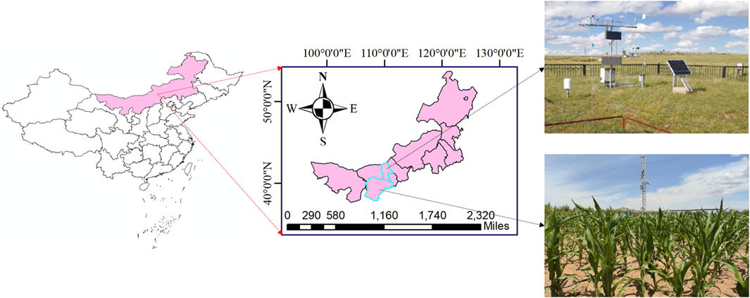
Figure 1. Location of the study area.
The Yinshanbeilu Grassland Eco-hydrology National Observation and Research Station is located in the Damao Banner, Baotou City, Inner Mongolia. The total area of the research station is about 1.3 km2, the altitude is 1,600 m, the annual mean temperature (Ta) of the location is 3.8°C, the annual mean wind speed is 5.3 m/s, the annual mean precipitation is 246 mm, the annual mean evaporation from the water surface is 2,200 mm, and the annual mean frost-free period is 110 days. The soils in the experimental site are chestnut soil. Due to differences in topography, parent material, water conditions, saline-alkali soil, and aeolian sand soil are formed in some areas. The overall amounts of potassium, phosphorus, and nitrogen in the soil were 2.5%, 0.08%–0.15%, and 0.1%–0.15%, respectively. Also, the pH of the soil ranged from 8 to 8.5. Grazing was the predominant land use, moderate-to-severe degradation had been widely distributed, and grassland overload in grazing regions was a major concern (Han et al., 2023).
The altitude of Suburga Township, Yijinholo Banner, Ordos City, is 1,456 m above sea level, the annual mean temperature (Ta) is 7.6°C, the average annual wind speed is 2.8 m/s, the average annual precipitation is 260 mm, the average annual evaporation from the water surface is 2,501 mm, and the average annual frost-free period is 160 days. The main crop grown in the area was maize. The climate type of the two areas is a mid-temperate and semi-arid continental monsoon climate and the soil texture is sandy loam.
2.2 Experimental details
The Krylov Needlegrass was the typical grassland group species in the Yinshanbeilu area, and the common species used were Artemisia frigida Willd, Leymus chinensis (Trin.) Tzvel., and Agropyron cristatum (L.) Gaertn (Han et al., 2022). The average height and coverage of vegetation was 40 cm and 35%, respectively (Miao et al., 2022). The growth periods of the grass in this study were divided into early (May 13–June 15), middle (June 15–August 15), and late stage (August 15–October 12).
Air temperature (Ta), relative humidity (RH), net radiation (Rn) and surface temperature (Ts) during grass growing season were measured by an ENVIS meteorological system (IMKO, Germany) at the Yinshanbeilu Grassland Eco-hydrology National Observation and Research Station. The meteorological observation instrument was installed at a height of 3.5 m. Air temperature and humidity sensors (HMP45C, Vasisla, Helsinki, Finland) were included, which were used to observe Ta and RH. In addition, Rn was observed by four-channel net radiation sensors (Kipp and Zonen, the Netherlands). The Ts was observed by an infrared radiometer (SI-111, Campbell Scientific, Inc., United States). The soil water content (SWC) at depths of 0–10 cm was measured. A tipping bucket rain gauge (TE525WS, Campbell Scientific Inc., United States) was used to measure precipitation (P) and stored after calculating the average value for 30 min. The Eddy covariance system (ECS) used in this study was manufactured by Licor Corporation, United States. The system mainly consisted of a three-dimensional ultrasonic anemometer (CSAT-3, Campbell Scientific, Logan, UT, United States), an infrared gas analyzer (LI-7500, Li-CORInc, United States), integrate, short and longwave radiation in one sensor (NR-LITE, Campbell Scientific), two soil heat flux plates, which were buried about 10 cm below the ground surface (HFP01, Campbell Scientific). The data acquisition (CR3000, Campbell Scientific) was at a frequency of 10 Hz with a measurement step of 30 min (8:00–18:00).
Maize (Fengtian 1,631) in Yijinholo Banner was planted in 1 May 2022 and harvested in 30 September 2022 with a planting density of 5,600 plants/acre. The experiment was conducted using a single-wing labyrinth drip irrigation laterals with 0.3 m emitter spacing, emitter flow rate of 3.6 L/h and wall thickness of 0.4 mm. The drip irrigation pipes were buried at 3–5 cm under the soil surface.
An automated weather station was installed in the middle of the maize field. Net radiation (Rn) was measured by a CNR-4 sensor (Kipp and Zonen, the Netherlands) at 3 m above ground. Air temperature and relative humidity were recorded with psychrometers HMP155A (Vaisala, Finland) at a height of 3 and 4 m above ground. The infrared thermometer (SI-111, Apogee, United States) was adjusted to the height of the crop canopy during the experiment and continuously measured the crop canopy temperature. Wind speed and direction were measured by a three cups anemometer A100L2 (MetOne, United States) at 3 m above ground. Soil heat flux was measured with a soil heat flux plate HFP01-L10 (Campbell Scientific, United States). All the sensors were connected to a data logger CR3000 (Campbell Scientific, United States) and all the data were sampled every 10 s, averaged every 10 min. The accuracy of all the sensors was validated before the installation. The maize field was surrounded by other similar crops and the installation height of the probes used to observe the air temperature and relative humidity was low (50–100 cm above the canopy), so, adequate fetch length can be met.
2.3 Methods
The energy balance equation could be expressed as Eq. 1 (Shi et al., 2021):
where, Rn is net radiation (W/m2), G is soil heat flux (W/m2), λET is latent heat flux (W/m2), H is sensible heat flux (W/m2).
Hourly latent heat flux of maize was obtained by the Bowen ratio energy balance (BREB) method (Yan et al., 2021) given by Eq. 2:
where, β is the Bowen ratio and can be expressed as Eq. 3:
where, ∆T is the air temperature gradient, ∆e is the actual vapor pressure gradient and λ is the psychrometric constant (kPa/°C).
Hourly λET of grassland was obtained by the Eddy covariance system (ECS).
The latent heat flux (λET) was calculated from the covariance between the vertical wind speed and the water vapor concentration, as shown in Eq. 4:
where, λET represents the latent heat flux (W/m2), ρ represents the air density (kg/m3), Cp is the specific heat of air (J/(kg·°C)), and
Energy balance closure analysis of the ECS is one of the main methods for analyzing the reliability of flux data, the energy balance ratio (EBR) was determined using Eq. 5:
where, EBR denotes the energy closure (%),G denotes the soil heat flux (W/m2), H denotes the sensible heat flux (W/m2), and Rn denotes the net radiation (W/m2).
The EBR during the observation period (May- October 2020) was approximately 85% (Figure 2). Li et al. (2018) analyzed the site energy closure of the Chinese flux network with R2 ranging from 0.51 to 0.93 and regression slopes from 0.54 to 0.88. The energy closure of this site is in a reasonable range compared to data from other sites.
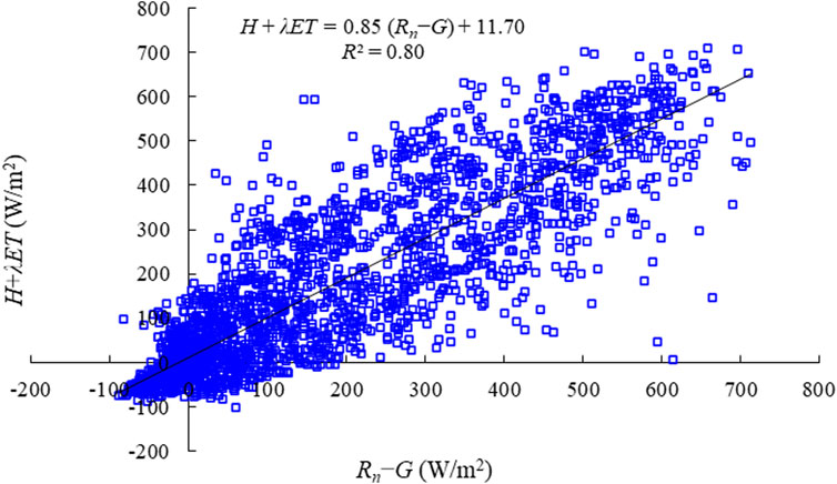
Figure 2. The energy balance ratio in May–October 2020.
2.4 Model description
2.4.1 Penman-Monteith model
The λET were calculated by the Penman-Monteith (P-M) model (Monteith, 1965) as Eq. 6:
where, VPD is the water vapor pressure difference (kPa), ρa is the density of air at atmospheric pressure (kg/m3), Cp is the specific heat of air [J/(kg·°C)], Δ is the slope of the curve relating saturated water vapor pressure and temperature (kPa/°C), rc is the canopy resistance parameter (s/m), ra is the aerodynamic resistance (s/m).
The ra was calculated by applying the logarithmic function of the wind speed. The equation (Perrier, 1975) are Eqs 7–9:
where, K is the von Karman constant (=0.41), z is the height of wind measurements (m), d is the zero plane displacement height (m), uz is the wind speed at height z (m/s), hc is the mean height of the crop (m).
2.4.2 Katerji-Perrier model
Katerji et al. (1983b) developed a linear relationship between the ratios rc/ra and r*/ra with the following relation (K-P model), as shown in Eq. 10:
where, a and b are empirical coefficients, r* is climatic resistance (s/m) and defined as Eq. 11:
While the K-P method and the P-M equation share similar hypotheses, the K-P method makes the assumption that the ae rodynamic resistance originates from the top of the canopy and that the “big leaf” is situated there. Thus, the following is a suggested aerodynamic resistance (Rana et al., 2005), as shown in Eq. 12.
where, hc is the reference crop height in this paper, z0 is the roughness length estimated as z0 = 0.1hc, d is the zero plane displacement estimated as d = 0.67hc, z is the height of measurements (m), uz is the wind speed at the height of z (m/s).
2.4.3 Garcıá-Santos model
The Garcıá-Santos (G-A) model is based on the Jarvis-Stewart model that calculates hourly canopy conductance. Only the Rn and VPD were considered in the model. The G-A canopy resistance model is expressed as follows (García-Santos et al., 2009):
where, gsm (mm/s), e1 (W/m2) and e2 (g/kg) are empirical coefficients which need experimental determination, VPD is the vapor pressure deficit (kPa).
2.5 Statistical evaluation
The statistical indices include the determination coefficient (R2), mean absolute error (MAE), Nash-Sutcliffe Efficiency (NSE) and root mean square error (RMSE), defined as shown in Eqs 14–16:
where, Ei represent the estimated values, Oi represent the observed values, O is the mean of observed values, n is the total number of semple.
3 Results
3.1 Meteorological data
The observed meteorological data during the growing periods of grass and maize plants are shown in Figure 3. The air temperature (Ta) and vapor pressure deficit (VPD) during grass growing season in 2020 (from 13 May 2020 to 5 October 2020) ranged from −4.49°C to 23.60°C and 0.04–2.29 kPa, with average values equaled 14.74°C and 0.78 kPa, respectively. Daily Rn ranged from 19.2 to 200.4 W/m2, with mean value of 116.1 W/m2. The daily wind speed (u) varied from 0.12 to 4.87 m/s, with the highest value of 4.87 m/s in the summer season.
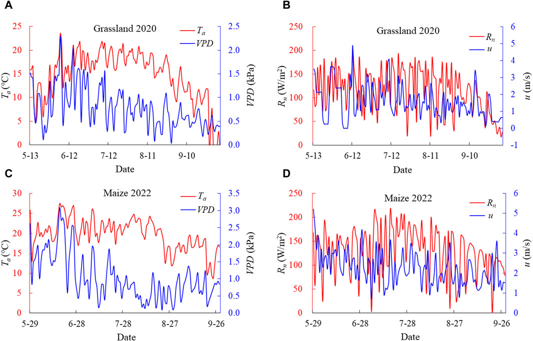
Figure 3. The variations of meteorological data during grass and maize growing season in 2020 and 2022, respectively. (A) Ta and VPD for grassland, (B) Rn and u for grassland, (C) Ta and VPD for maize, (D) Rn and u for maize.
The Ta and VPD ranged from 8.71°C to 27.53°C and 0.09–3.08 kPa, with average values equaled 19.79°C and 1.03 kPa during maize growing season in 2022 (from 29 May 2022 to 28 September 2022). Daily Rn ranged from 0.17 to 216.31 W/m2, with mean value of 129.95 W/m2. The value of u varied from 0.69 to 5.20 m/s, with mean value of 2.24 m/s.
3.2 Estimation of latent heat flux
3.2.1 Calibration of the Katerji-Perrier model
The K-P model was calibrated based on the data from grassland and maize fields individually. The model coefficients a and b were yielded from the linear regression between rc/ra and r*/ra for each site. In this study, the K-P model was calibrated using hourly data during ten typical clear days, which were randomly chosen from the experimental periods at the grassland and maize fields. The rc was computed by inverting the Eq. 6 with the measured λET. The Figure 4, Eqs 17, 18 represent the results of the linear regression between the rc/ra and r*/ra for the grassland and maize. The regression coefficients a and b of the K-P model were 0.67 and −1.74 for grassland and 0.74 and 4.8 for maize, respectively. The determination coefficients (R2) were 0.91 and 0.88 for grassland and maize, respectively. Moreover, the results of some previous studies for the calibration results of the K-P model are summarized as shown in Table 1.
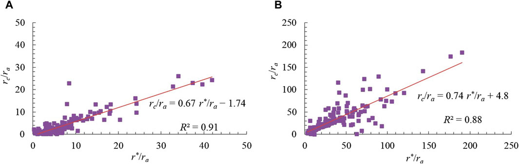
Figure 4. Calibration plots for K-P model parameters in grassland and maize field. (A) Grassland, (B) Maize.
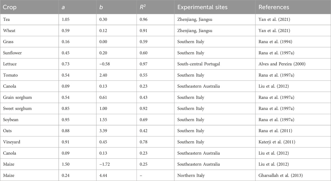
Table 1. Summary of the calibration coefficients a and b of the K-P model for different study areas or crops conducted by previous studies.
3.2.2 Calibration of the Garcıá-Santos model
The parameters of G-A model were calibrated using the least squares method through hourly scale data from ten typical clear days. The basic principle of the least squares method is to estimate the model parameters on the criterion of minimizing the sum of squares of the errors. Data for the days used to calibrate the model were not used for the validation of modeled rc and λET. The rc was computed by inverting the Eq. 6 with the measured λET. The optimized parameters gsm (mm/s), e1 (W/m2) and e2 (g/kg) as well as the degree of variance explained (%) by the model for grasslands and maize are listed in Table 2.

Table 2. Optimized values of parameters (gsm, e1, e2) in the G-A model and the variance explained by the model for grassland and maize.
The results of some previous studies for the calibration results of the G-A model are summarized as shown in Table 3.

Table 3. Summary of calibration coefficients gsm, e1 and e2 of the G-A model for different crops of previous studies.
3.3 Evaluation of the canopy resistance model
For the K-P model, the slope of the linear relationships between estimated and measured λET values was 0.95 for grassland and 0.97 for maize during the whole growing period (Figures 5A, B). Thus, the K-P model underestimated λET slightly both in the cases of grassland and maize. The intercepts were 0.52 and 3.75, with RMSE of 37.3 and 28.1 W/m2 for grassland and maize, respectively.
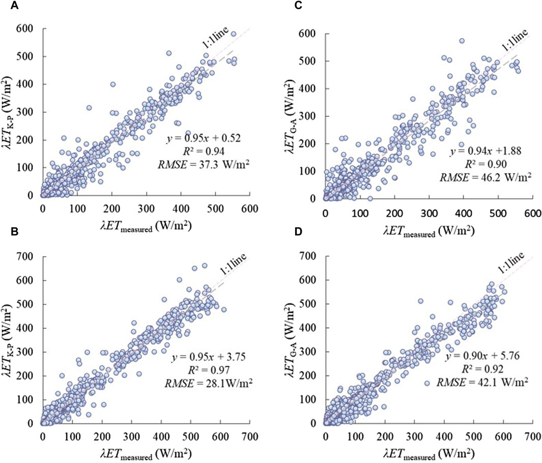
Figure 5. Comparison between the λET of estimated values by two canopy resistance parameter sub-models and the measured values by Bowen ratio balance method and Eddy covariance system for grassland and maize. (A) K-P for grassland, (B) K-P for maize, (C) G-A for grassland, (D) G-A for maize.
For the G-A model, the slope of the linear relationships between estimated and measured λET was 0.94 for the grassland (Figure 5C) with RMSE of 46.2 W/m2 and NSE of 0.88, indicating that the G-A model underestimated the λET significantly, while the slope was 0.92 for the maize (Figure 5D) with RMSE of 42.1 W/m2 and NSE of 0.90.
According to the statistics presented in Table 4, the best NSE value (=0.96) was obtained with the K-P model for maize. The worst NSE value (=0.88) was obtained with the G-A model for grassland, despite the G-A model giving an excellent NSE value of 0.90 for maize. The best MAE, acquired on maize for K-P method, was equal to 19.3 W/m2.
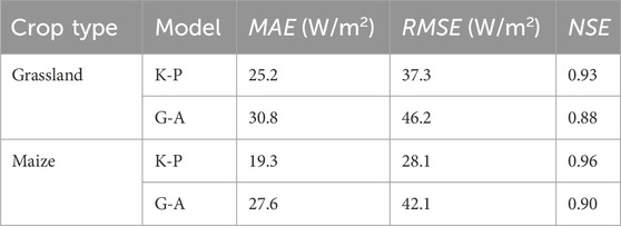
Table 4. Statistical indices between estimated and measured λET of grassland and maize field.
4 Discussion
In this study, the K-P and G-A models were used to simulate the λET based on the P-M model during the growing periods of grass and maize in the arid region of Northwest China. The estimated λET values of the K-P and G-A model (λETK-P and λETG-A) were smaller than the measured λET for grassland. The possible reason might due to the effects of changes in soil moisture and crop LAI on canopy resistance during the growing periods were not taken into account. Li et al. (2015) conducted experimental studies on maize and grape in the northern region of China based on twelve rc models, and the results showed that the K-P model simulation results were more superior. Simulations of λET in olive trees by Margonis et al. (2018) showed that the K-P model underestimated λET by about 9.8%. The results of all the above studies were consistent with the results of the present study.
The relationships between meteorological factors and absolute value of error of the K-P and G-A models in estimating λET were analyzed, it was found that VPD was the main factor affecting the model errors (Figure 6), while other factors have little influence. For the grassland, when the VPD value exceeds 1 kPa, the error increased with the increasing in VPD for both models. Shi et al. (2008) experimented with the broad-leaved Korean pine forest in the Changbai Mountains in the south-east of Jilin Province, China, pointed out that when the value of VPD was more than 1.5 kPa, the accuracy of estimation tended to below.
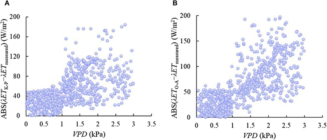
Figure 6. The influence of VPD on the absolute value of error of the K-P and G-A models in estimation of λET of grassland. λETK-P represents the estimated latent heat flux by the K-P model. λETG-A represents the estimated latent heat flux by the G-A model. (A) K-P for grassland, (B) G-A for grassland.
For the maize field, when the VPD exceeded 1.5 kPa, the absolute value of error increased with the increasing in VPD (Figure 7). Results similar to this study were reported by Katerji et al. (2011) on the effect of VPD in the values of evapotranspiration which stated that when the value of VPD was more than 2 kPa, the values of the estimated evapotranspiration were larger than the measured evapotranspiration. The greater abundance of water vapor in July and August in maize field may be another reason for the underestimation of λET by the K-P model. Most of the λETG-A were smaller than the λETmeasured during the growing period of maize especially when the λETmeasured was high. Srivastava et al. (2018) conducted a preliminary study on the effect of VPD in the value of evapotranspiration in the West Bengal, India, pointing out that when the value of VPD was in the range of 1.23–3.0 kPa, the accuracy of estimation tended to below. The more abundant water vapor in the maize field in July and August may also contributed to the large errors in the simulation results of the G-A model simulation results.
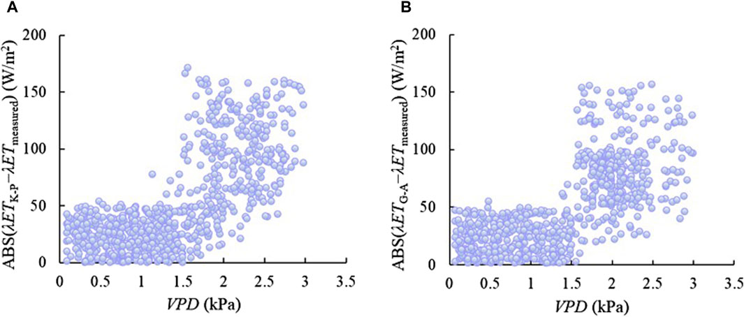
Figure 7. The influence of VPD on the absolute value of error of the K-P and G-A models in estimation of λET of maize. λETG-A represents the estimated latent heat flux by the G-A model. (A) K-P for maize, (B) G-A for maize.
Generally, the K-P model were more accurate in simulating the λET of grassland and maize field in Northwest China.
5 Conclusion
In this study, two rc models (K-P and G-A) were applied and compared for the λET estimation. Based on the analysis of statistical indices, the following conclusions were made.
The K-P model was the superior method for predicting hourly λET of grassland and maize. The G-A model was a good alternative approach for estimating λET of grassland and maize. For the K-P model, the RMSE were equal 37.3–28.1 W/m2 for grassland and maize, respectively. For the G-A model, the RMSE values was 46.2 W/m2 for grassland and 42.1 W/m2 for maize during the whole growing period. The results showed that the R2 of the simulation results of the two rc models (K-P and G-A) were above 0.8, but the K-P model simulation was better. Both the K-P and G-A models underestimated the λET of grassland and maize.
The absolute error of the two models increased with the increasing in VPD. For the K-P model, the effect of LAI changes on crop canopy resistance during crop growth was not considered, which would have made the model performance slightly worse in the early part of the growing season. For the G-A model, due to the limitations of the modeling theory, only the effects of mete-orological factors such as Rn and VPD were taken into account, while the effect of soil on evapotranspiration was not considered, which would have made the model performance slightly worse (Li et al., 2015). Matheny et al. (2014)conducted a preliminary study on the prediction of evapotranspiration in the North Ameri-can, pointing out that most rc models under water stress conditions have difficulty in re-solving the dynamics of λET due to errors in calculating surface resistance.
Data availability statement
The original contributions presented in the study are included in the article/supplementary material, further inquiries can be directed to the corresponding author.
Author contributions
BW: Writing–original draft. HY: Writing–review and editing. HZ: Funding acquisition, Writing–review and editing. JW: Writing–review and editing. DT: Writing–review and editing. CZ: Writing–review and editing. XZ: Writing–review and editing. GW: Writing–review and editing. IL: Writing–review and editing. YL: Writing–review and editing.
Funding
The author(s) declare that financial support was received for the research, authorship, and/or publication of this article. This study was financially supported by the Science and Technology Xingmeng Action Key Special Project (2021EEDSCXSFQZD010); the National Key R&D Program (2021YFC3201103); the Natural Science Foundation of China (52121006, U2243228, 1509107, 42177065); the Key R&D Project of Jiangsu Province (BE2022351); Yinshanbeilu Grassland Eco-hydrology National Observation and Research Station, Institute of Water Resources and Hydropower Research, Beijing 100038, China (YSS2022011).
Conflict of interest
The authors declare that the research was conducted in the absence of any commercial or financial relationships that could be construed as a potential conflict of interest.
Publisher’s note
All claims expressed in this article are solely those of the authors and do not necessarily represent those of their affiliated organizations, or those of the publisher, the editors and the reviewers. Any product that may be evaluated in this article, or claim that may be made by its manufacturer, is not guaranteed or endorsed by the publisher.
References
Alves, I., and Pereira, L. S. (2000). Modelling surface resistance from climatic variables? Agric. Water Manag. 42 (3), 371–385. doi:10.1016/s0378-3774(99)00041-4
Deng, M. (2018). "Three Water Lines" strategy: its spatial patterns and effects on water resources allocation in northwest China.
García-Santos, G., Bruijnzeel, L. A., and Dolman, A. J. (2009). Modelling canopy conductance under wet and dry conditions in a subtropical cloud forest. Agric. For. Meteorology 149 (10), 1565–1572. doi:10.1016/j.agrformet.2009.03.008
Gharsallah, O., Facchi, A., and Gandolfi, C. (2013). Comparison of six evapotranspiration models for a surface irrigated maize agro-ecosystem in Northern Italy. Agric. Water Manag. 130, 119–130. doi:10.1016/j.agwat.2013.08.009
Guo, B., Kong, W. H., and Jiang, L. (2018). Dynamic monitoring of vulnerability and quantitative analysis of driving factors in northwest arid desert ecosystem. Nat. Resour. 33, 412–424. doi:10.11849/zrzyxb.20170068
Guo, Z., Wu, Y., Li, Q., Gu, F., Liu, X., Li, Y., et al. (2022). Application of six canopy resistance models for estimating winter wheat evapotranspiration. Trans. Chin. Soc. Agric. Eng. 38 (12), 109–117. doi:10.11975/j.issn.1002-6819.2022.12.013
Han, X., Zhang, B. Z., Liu, T. J., Wang, J., Zhou, Q. Y., and Che, Z. (2023). The effect of time scales on the distribution of evapotranspiration and driving factors in desert grasslands. Agric. Water Manag. 284, 108348. doi:10.1016/j.agwat.2023.108348
Han, X., Zhou, Q. Y., Zhang, B. Z., Che, Z., Wei, Z., Qiu, R. J., et al. (2022). Real-time methods for short and medium-term evapotranspiration forecasting using dynamic crop coefficient and historical threshold. J. Hydrology 606, 127414. doi:10.1016/j.jhydrol.2021.127414
Haofang, Y., Baoshan, Z., Chuan, Z., Song, H., Hanwen, F., Jianjun, Y., et al. (2019). Estimating cucumber plants transpiration by Penman-Monteith model in Venlo-type greenhouse. Trans. Chin. Soc. Agric. Eng. doi:10.11975/j.issn.1002-6819.2019.08.018
Jarvis, P. (1976). The interpretation of the variations in leaf water potential and stomatal conductance found in canopies in the field. Philosophical Trans. R. Soc. Lond. B, Biol. Sci. 273 (927), 593–610. doi:10.1098/rstb.1976.0035
Katerji, N., Perrier, A., and Oulid-Aïssa, A. K. (1983a). Exploration au champ et interprétation de la variation horizontale et verticale de la résistance stomatique: cas d'une culture de luzerne (Medicago sativa L.). Agronomie 3 (9), 847–856. doi:10.1051/agro:19830904
Katerji, N., Perrier, A., Renard, D., and Aissa, A. K. O. (1983b). Modélisation de l'évapotranspiration réelle ETR d'une parcelle de luzerne: rôle d'un coefficient cultural. Agronomie 3 (6), 513–521. doi:10.1051/agro:19830603
Katerji, N., Rana, G., and Fahed, S. (2011). Parameterizing canopy resistance using mechanistic and semi-empirical estimates of hourly evapotranspiration: critical evaluation for irrigated crops in the Mediterranean. Hydrol. Process. 25 (1), 117–129. doi:10.1002/hyp.7829
Lecina, S., Martínez-Cob, A., Pérez, P. J., Villalobos, F. J., and Baselga, J. J. (2003). Fixed versus variable bulk canopy resistance for reference evapotranspiration estimation using the Penman-Monteith equation under semiarid conditions. Agric. Water Manag. 60 (3), 181–198. doi:10.1016/s0378-3774(02)00174-9
Li, L. (2019). Application of different canopy resistance models to evapotranspiration in maize ecosystems in semi-arid areas. Lanzhou University.
Li, S. E., Hao, X. M., Du, T. S., Tong, L., Zhang, J. H., and Kang, S. Z. (2014). A coupled surface resistance model to estimate crop evapotranspiration in arid region of northwest China. Hydrol. Process. 28 (4), 2312–2323. doi:10.1002/hyp.9768
Li, S. E., Zhang, L., Kang, S. Z., Tong, L., Du, T. S., Hao, X. M., et al. (2015). Comparison of several surface resistance models for estimating crop evapotranspiration over the entire growing season in arid regions. Agric. For. Meteorology 208, 1–15. doi:10.1016/j.agrformet.2015.04.002
Li, Z., Yu, G., and Wen, X. (2018). Evaluation of the energy balance closure status of the China flux observation network (ChinaFLUX). Sci. China Series D Earth Sci. 2004 (S2), 46–56.
Liu, G. S., Liu, Y., Hafeez, M., Xu, D., and Vote, C. (2012). Comparison of two methods to derive time series of actual evapotranspiration using eddy covariance measurements in the southeastern Australia. J. Hydrology 454, 1–6. doi:10.1016/j.jhydrol.2012.05.011
Margonis, A., Papaioannou, G., Kerkides, P., Kitsara, G., and Bourazanis, G. (2018). Canopy resistance and actual evapotranspiration over an olive orchard. Water Resour. Manag. 32 (15), 5007–5026. doi:10.1007/s11269-018-2119-x
Matheny, A. M., Bohrer, G., Stoy, P. C., Baker, I. T., Black, A. T., Desai, A. R., et al. (2014). Characterizing the diurnal patterns of errors in the prediction of evapotranspiration by several land-surface models: an NACP analysis. J. Geophys. Research-Biogeosciences 119 (7), 1458–1473. doi:10.1002/2014jg002623
Miao, H. L., Wang, A. T., Zhang, R. Q., Li, J. R., and Gao, T. M. (2022). Characteristics of wind regime and drift potential of the desert steppe in northern slope of Yinshan Mountains. Inner Mongolia. J. Arid Land Resour. Environ 36, 102–110. doi:10.13448/j.cnki.jalre.2022.098
Niu, G., Li, Y. P., Huang, G. H., Liu, J., and Fan, Y. R. (2016). Crop planning and water resource allocation for sustainable development of an irrigation region in China under multiple uncertainties. Agric. Water Manag. 166, 53–69. doi:10.1016/j.agwat.2015.12.011
Perrier, A. (1975). Etude physique de l'évapotranspiration dans les conditions naturelles. III. Evapotranspiration réelle et potentielle des couverts végétaux.
Rana, G., Katerji, N., and de Lorenzi, F. (2005). Measurement and modelling of evapotranspiration of irrigated citrus orchard under Mediterranean conditions. Agric. For. Meteorology 128 (3-4), 199–209. doi:10.1016/j.agrformet.2004.11.001
Rana, G., Katerji, N., Ferrara, R. M., and Martinelli, N. (2011). An operational model to estimate hourly and daily crop evapotranspiration in hilly terrain: validation on wheat and oat crops. Theor. Appl. Climatol. 103 (3-4), 413–426. doi:10.1007/s00704-010-0308-5
Rana, G., Katerji, N., Mastrorilli, M., and Moujabber, M. (1997a). A model for predicting actual evapotranspiration under soil water stress in a Mediterranean region. Theor. Appl. Climatol. 56 (1-2), 45–55. doi:10.1007/bf00863782
Rana, G., Katerji, N., Mastrorilli, M., and Moujabber, M. E. (1994). Evapotranspiration and canopy resistance of grass in a Mediterranean region. Theor. Appl. Climatol. 50 (1), 61–71. doi:10.1007/bf00864903
Rana, G., Katerji, N., Mastrorilli, M., Moujabber, M. E., and Brisson, N. (1997b). Validation of a model of actual evapotranspiration for water stressed soybeans. Agric. For. Meteorology 86 (3-4), 215–224. doi:10.1016/s0168-1923(97)00009-9
Rana, G., Katerji, N., and Perniola, M. (2001). Evapotranspiration of sweet sorghum: a general model and multilocal validity in semiarid environmental conditions. Water Resour. Res. 37 (12), 3237–3246. doi:10.1029/2001wr000476
Shi, T. T., Guan, D. X., Wang, A. Z., Wu, J. B., Jin, C. J., and Han, S. J. (2008). Comparison of three models to estimate evapotranspiration for a temperate mixed forest. Hydrol. Process. 22 (17), 3431–3443. doi:10.1002/hyp.6922
Shi, Y., Shi, H., Cui, Y., Hong, D., and Zhu, H. (2021). Variation of water use efficiency in a paddy field in the middle and lower reaches of the Yangtze River using eddy covariance method. Trans. Chin. Soc. Agric. Eng. 37 (4), 130–139. doi:10.11975/j.issn.1002-6819.2021.04.016
Srivastava, R. K., Panda, R. K., Chakraborty, A., and Halder, D. (2018). Comparison of actual evapotranspiration of irrigated maize in a sub-humid region using four different canopy resistance based approaches. Agric. Water Manag. 202, 156–165. doi:10.1016/j.agwat.2018.02.021
Todorovic, M. (1999). Single-layer evapotranspiration model with variable canopy resistance. J. Irrigation Drainage Eng. 125 (5), 235–245. doi:10.1061/(asce)0733-9437(1999)125:5(235)
Xu, L., Xiao, K., and Wei, R. (2020). Irrigation models for the tomatoes cultivated in organic substrate based on greenhouse environment and crop growth. Trans. Chin. Soc. Agric. Eng. 36 (10), 189–196. doi:10.11975/j.issn.1002-6819.2020.10.023
Yan, H., Zhou, Y., Zhang, J., Wang, G., Zhang, C., Yu, J., et al. (2022a). Parametrization of canopy resistance and simulation of latent heat fluxes for typical crops in southern Jiangsu Province. Trans. Chin. Soc. Agric. Eng. 38 (9), 101–107. doi:10.11975/j.issn.1002-6819.2022.09.011
Yan, H. F., Deng, S. S., Zhang, C., Wang, G. Q., Zhao, S., Li, M., et al. (2023). Determination of energy partition of a cucumber grown Venlo-type greenhouse in southeast China. Agric. Water Manag. 276, 108047. doi:10.1016/j.agwat.2022.108047
Yan, H. F., Huang, S., Zhang, J. Y., Zhang, C., Wang, G. Q., Li, L. L., et al. (2022b). Comparison of shuttleworth-wallace and dual crop coefficient method for estimating evapotranspiration of a tea field in southeast China. Agriculture-Basel 12 (9), 1392. doi:10.3390/agriculture12091392
Yan, H. F., Shi, H. B., Hiroki, O., Zhang, C., Xue, Z., Cai, B., et al. (2015). Modeling bulk canopy resistance from climatic variables for predicting hourly evapotranspiration of maize and buckwheat. Meteorology Atmos. Phys. 127 (3), 305–312. doi:10.1007/s00703-015-0369-1
Yan, H. F., Yu, J. J., Zhang, C., Wang, G. Q., Huang, S., and Ma, J. M. (2021). Comparison of two canopy resistance models to estimate evapotranspiration for tea and wheat in southeast China. Agric. Water Manag. 245, 106581. doi:10.1016/j.agwat.2020.106581
Yu, J. (2022). Characterization and simulation of water-heat flux changes in typical farmland in the southern Jiangsu region. Jiangsu University. doi:10.27170/d.cnki.gjsuu.2021.000315
Zhang, B., Xu, D., Liu, Y., and Chen, H. (2015). Review of multi-scale evapotranspiration estimation and spatio-temporal scale expansion. Trans. Chin. Soc. Agric. Eng. 31 (6), 8–16. doi:10.3969/j.issn.1002-6819.2015.06.002
Keywords: grassland, maize, heat flux, Northwest region, Penman-Monteith model
Citation: Wang B, Yan H, Zheng H, Wu J, Tian D, Zhang C, Zhu X, Wang G, Lakhiar IA and Liu Y (2024) Estimation of latent heat flux of pasture and maize in arid region of Northwest China based on canopy resistance modeling. Front. Environ. Sci. 12:1397704. doi: 10.3389/fenvs.2024.1397704
Received: 10 April 2024; Accepted: 22 July 2024;
Published: 01 August 2024.
Edited by:
Heping Liu, Washington State University, United StatesReviewed by:
Umar Farooq, Foundation Euro-Mediterranean Center on Climate Change (CMCC), ItalyPeishi Jiang, Pacific Northwest National Laboratory (DOE), United States
Copyright © 2024 Wang, Yan, Zheng, Wu, Tian, Zhang, Zhu, Wang, Lakhiar and Liu. This is an open-access article distributed under the terms of the Creative Commons Attribution License (CC BY). The use, distribution or reproduction in other forums is permitted, provided the original author(s) and the copyright owner(s) are credited and that the original publication in this journal is cited, in accordance with accepted academic practice. No use, distribution or reproduction is permitted which does not comply with these terms.
*Correspondence: Haofang Yan, eWFuaGFvZmFuZ3loZkAxNjMuY29t