High-precision prediction of microalgae biofuel production efficiency: employing ELG ensemble method

Microalgae biofuels are considered a significant source of future renewable energy due to their efficient photosynthesis and rapid growth rates. However, practical applications face numerous challenges such as variations in environmental conditions, high cultivation costs, and energy losses during production. In this study, we propose an ensemble model called ELG, integrating Empirical Mode Decomposition (EMD), Long Short-Term Memory (LSTM), and Gradient Boosting Machine (GBM), to enhance prediction accuracy. The model is tested on two primary datasets: the EIA (U.S. Energy Information Administration) dataset and the NREL (National Renewable Energy Laboratory) dataset, both of which provide extensive data on biofuel production and environmental conditions. Experimental results demonstrate the superior performance of the ELG model, achieving an RMSE of 0.089 and MAPE of 2.02% on the EIA dataset, and an RMSE of 0.1 and MAPE of 2.21% on the NREL dataset. These metrics indicate that the ELG model outperforms existing models in predicting the efficiency of microalgae biofuel production. The integration of EMD for preprocessing, LSTM for capturing temporal dependencies, and GBM for optimizing prediction outputs significantly improves the model’s predictive accuracy and robustness. This research, through high-precision prediction of microalgae biofuel production efficiency, optimizes resource allocation and enhances economic feasibility. It advances technological capabilities and scientific understanding in the field of microalgae biofuels and provides a robust framework for other renewable energy applications.

1 Introduction

The accurate prediction of microalgae biofuel production efficiency is essential for optimizing sustainable biofuel technologies and addressing challenges in large-scale applications. Microalgae, as a sustainable biological resource, are considered a significant source of future biofuels due to their efficient photosynthesis and rapid growth rate Sathya et al. (2023). The efficiency of microalgae biofuel production refers to the efficiency of converting photosynthesis into biofuels under specific conditions, including the growth rate of biomass and the proportion converted into fuel Huang et al. (2023). Despite the potential of microalgae for efficient CO2 conversion, practical applications face numerous challenges such as variations in environmental conditions, high cultivation costs, and energy losses during production. Additionally, the instability and difficulty in predicting production efficiency are major obstacles in the microalgae biofuel industry Subhash et al. (2022); Sun et al. (2023). To address these challenges, accurate prediction models are crucial. In recent years, deep learning technologies have shown great potential in improving the prediction accuracy of microalgae biofuel production efficiency due to their powerful data processing and pattern recognition capabilities. Deep learning models such as Convolutional Neural Networks (CNNs) and Recurrent Neural Networks (RNNs) have been successfully applied to monitor the growth status of microalgae, predict biomass production, and optimize operating parameters of bioreactors Chong et al. (2024). These studies not only improve production efficiency but also reduce the production costs of biofuels. Time series forecasting plays a crucial role in the study of microalgae biofuel production efficiency. The growth of microalgae biomass is closely related to environmental factors such as light, temperature, and nutrient supply, which vary over time, forming typical time series data Sultana et al. (2022); Dong et al. (2024). Through accurate time series analysis and forecasting models, researchers can predict the growth trends of microalgae under specific environmental conditions, thereby adjusting cultivation strategies in advance, optimizing resource allocation, and ensuring the sustainable and efficient production of biofuels. Furthermore, time series forecasting also facilitates real-time monitoring and feedback on the production process, enhancing production management automation.

Recent advancements in research have demonstrated the widespread applicability of deep learning and machine learning models in predicting microalgae biofuel production efficiency. One study utilized a Convolutional Neural Network (CNN) model to analyze image data of microalgae biomass production Syed et al. (2024). By employing automated image processing techniques, the study captured key visual features during microalgae growth to predict biomass accumulation. While this method excelled in image recognition and feature extraction, it failed to adequately consider the time-series impact of environmental parameters, limiting its applicability in dynamic prediction scenarios. Another study utilized Long Short-Term Memory (LSTM) networks to model time-series data of microalgae biomass, focusing particularly on environmental factors such as light and temperature’s influence on biomass production Liu et al. (2022). This model effectively addressed temporal dependency issues, improving prediction accuracy. However, the computational demands of LSTM models for handling nonlinear and highly complex data resulted in lower efficiency in processing large-scale data. A third study employed the Random Forest (RF) algorithm to forecast microalgae biomass output Ma et al. (2023). Leveraging historical production data to predict future yields, the model demonstrated high accuracy and good interpretability. Despite Random Forest’s strong performance in multi-parameter environments, it tends to overfit when dealing with very large datasets and exhibits high sensitivity to outliers, potentially affecting the stability of prediction results. Lastly, a study explored a prediction model based on Support Vector Machine (SVM), focusing on predicting microalgae biofuel production from biochemical parameters Sonmez et al. (2022). SVM, chosen for its excellent performance on small sample data, effectively identified yield differences under different biochemical conditions. However, SVM’s scalability and flexibility are limited when facing large-scale or high-dimensional datasets, which could be a limiting factor in practical applications. Each of these studies has its strengths but also limitations, especially in handling large-scale, complex, and dynamic datasets. These challenges underscore the need for further integration and optimization of existing technologies to more comprehensively address the prediction of microalgae biofuel production efficiency.

Building upon the identified shortcomings of the aforementioned approaches, we propose an ensemble model called ELG(EMD-LSTM-GBM), integrating Empirical Mode Decomposition (EMD), Long Short-Term Memory (LSTM), and Gradient Boosting Machine (GBM). The EMD component preprocesses the data, extracting crucial trends and periodic features to prepare for subsequent deep learning analysis. LSTM captures the temporal dependencies of the processed data, effectively predicting biofuel production efficiency. Finally, GBM optimizes the output of LSTM, further enhancing prediction accuracy and model generalization. Compared to the existing models, our ELG model demonstrates superior performance in handling large-scale, complex datasets, effectively addressing the limitations identified in CNN, LSTM, RF, and SVM models. Integrating these three techniques not only enables more precise prediction of microalgae biofuel production efficiency but also enhances adaptability and robustness, especially in dynamic and multi-dimensional data environments. The model’s design allows us to leverage the multi-layered characteristics of time series data and effectively handle nonlinear and complex patterns within the data. Through this integrated approach, we anticipate significant improvements in prediction accuracy, providing scientific basis and technical support for the regulation and optimization of microalgae biofuel production.

In this study, we address the application of time series analysis in predicting microalgae biofuel production efficiency and propose a novel integrated model, demonstrating its significant contributions. Specifically, our main contributions encompass three aspects:

$•$ We introduce a novel integrated model that combines Empirical Mode Decomposition (EMD), Long Short-Term Memory (LSTM), and Gradient Boosting Machine (GBM). This integration enables us to leverage the strengths of each component: EMD for preprocessing data and extracting key features, LSTM for capturing temporal dependencies, and GBM for optimizing prediction outputs. By combining these techniques, our model offers improved prediction accuracy and robustness.

$•$ Through extensive experimentation and validation, we showcase the superior predictive performance of our integrated model compared to existing approaches. By effectively capturing the complex dynamics of microalgae biofuel production, our model achieves higher accuracy in forecasting production efficiency, thereby providing valuable insights for optimization strategies.

$•$ Our study contributes to advancing both scientific understanding and technological capabilities in the field of microalgae biofuel production. By demonstrating the efficacy of integrating time series analysis techniques, deep learning, and machine learning algorithms, we pave the way for more sophisticated and effective approaches to predicting and optimizing biofuel production processes.

The remainder of this paper is organized as follows. Section 2 reviews related work, discussing the role of ensemble learning in energy forecasting and the application of traditional predictive models in biofuel production. Section 3 details the methodology of our proposed ELG model, including the integration of Empirical Mode Decomposition (EMD), Long Short-Term Memory (LSTM) networks, and Gradient Boosting Machine (GBM). Section 4 describes the datasets and experimental setup, followed by a presentation of the experimental results and their analysis. Finally, Section 5 concludes the paper, summarizing our findings and suggesting directions for future research.

2 Related work

2.1 The role of ensemble learning in energy forecasting

Integrated learning, as a powerful data analysis tool, has been extensively researched in the field of energy prediction, especially in forecasting the generation of renewable energies such as wind and solar power Dong et al. (2019). For instance, in a study on wind energy prediction, researchers utilized ensemble methods such as Random Forest and Gradient Boosting Machine to enhance prediction accuracy under complex weather conditions Dubey et al. (2022); Wang et al. (2024). This research extensively analyzed the performance of various models such as Support Vector Machine (SVM), Artificial Neural Networks (ANN), and Decision Trees (DT) when used individually compared to when integrated, showing that ensemble models generally provided lower prediction errors and higher reliability Yao and Liu (2024). In the domain of solar power generation forecasting, another study employed a Stacked Regression model combined with multiple base prediction models such as Linear Regression, Support Vector Regression, and Neural Networks Elsaraiti and Merabet (2022); Gao et al. (2023). By integrating outputs from various base models using a secondary learning model, this approach effectively improved adaptability to changes in solar radiation and other environmental factors. The study emphasized the advantages of ensemble learning in handling prediction variability caused by environmental factors, providing detailed model evaluations and validation processes to demonstrate its benefits in practical applications Bijitha and Nath (2022); Maya et al. (2022). Furthermore, integrated learning techniques have also been applied to predict biomass energy production, where one study integrated time series analysis and machine learning methods to address the seasonal and stochastic characteristics of biomass energy production Drożdż et al. (2022); Tian et al. (2023). By combining outputs from Seasonal Autoregressive models with multiple nonlinear prediction models, this research enhanced prediction accuracy while also providing data support for biomass energy supply chain management. These examples illustrate that integrated learning not only demonstrates significant advantages in improving prediction accuracy but also exhibits unique capabilities in handling data uncertainty and nonlinearity. This approach can provide more stable and reliable decision support for energy prediction, making it a key factor in driving the development of energy prediction technology.

2.2 Application of traditional predictive models in biofuel production

In the prediction of biofuel production efficiency, traditional forecasting models such as Autoregressive Moving Average (ARMA), Seasonal Autoregressive Integrated Moving Average (SARIMA), and exponential smoothing methods have demonstrated practical utility Dong et al. (2022). These models utilize historical data series to forecast future production trends and output, typically performing best when data exhibit linear relationships Sharma et al. (2023). For instance, research indicates that the ARMA model effectively predicts biofuel production with stable seasonal patterns, such as ethanol production from corn. In a study focusing on U.S. corn ethanol production, the ARMA model accurately forecasted production for the upcoming months based on historical data, demonstrating relatively high accuracy in short-term predictions Yu et al. (2022). Moreover, the Seasonal Autoregressive Integrated Moving Average (SARIMA) model is employed to forecast biofuel production with clear seasonality and non-stationary data Hoang et al. (2023); Ma and Chen (2024). For example, in a forecast study concerning seasonal fluctuations in demand and supply of biodiesel, the SARIMA model adeptly captured seasonal fluctuations and provided accurate predictions for future supply trends over several seasons Jiang et al. (2022). Exponential smoothing is another common forecasting method, predicting future trends by assigning diminishing weights to old observed results Svetunkov et al. (2022). Particularly effective in the biofuel industry, it addresses demand forecasting and inventory management issues, as it rapidly adapts to demand changes and provides real-time forecast updates.

Despite the practicality demonstrated by these traditional methods in biofuel production and demand forecasting, they often face limitations when handling large-scale or complex datasets. As data volume and complexity increase, and with the diversity of factors influencing production processes, single traditional models increasingly struggle to meet the demand for precise forecasts. This prompts researchers to transition towards machine learning and more advanced statistical methods to enhance prediction accuracy and adaptability.

3 Methods

3.1 Overview of our network

This study devised an ensemble learning model to enhance the accuracy of predicting microalgae biofuel production efficiency. The proposed ELG model integrates three core components: Empirical Mode Decomposition (EMD), Long Short-Term Memory (LSTM), and Gradient Boosting Machine (GBM), each carefully selected and configured to address specific data features and improve overall predictive performance. To begin, raw time series data underwent preprocessing using EMD, which decomposes the data into multiple Intrinsic Mode Functions (IMFs). EMD effectively isolates intrinsic fluctuation patterns and trends within the data, enabling the extraction of meaningful periodicities. Processed through EMD, the data revealed dynamic variations in the production process, providing stable and reliable inputs for subsequent analysis. The extracted IMFs are then fed into the LSTM model. LSTM, adept at handling time series data with long-term dependencies, is responsible for capturing the temporal relationships within the data, allowing for the accurate forecasting of future biofuel production efficiency. Its ability to memorize and leverage historical information is crucial for predicting microalgae biofuel production efficiency, influenced by various interrelated factors. Finally, the predictions generated by the LSTM are refined using the GBM model. GBM reduces prediction errors and enhances model adaptability and accuracy by iteratively optimizing weak learners, such as decision trees. This final stage is critical as it boosts the model’s overall performance by addressing the residual errors from the LSTM’s output. Its integration significantly enhances the model’s explanatory power and predictive accuracy for complex biofuel production processes. Figure 1 provides a detailed flow chart of the ELG model, illustrating the step-by-step data processing through each of the core components (EMD, LSTM, GBM) and their interactions.

Figure 1

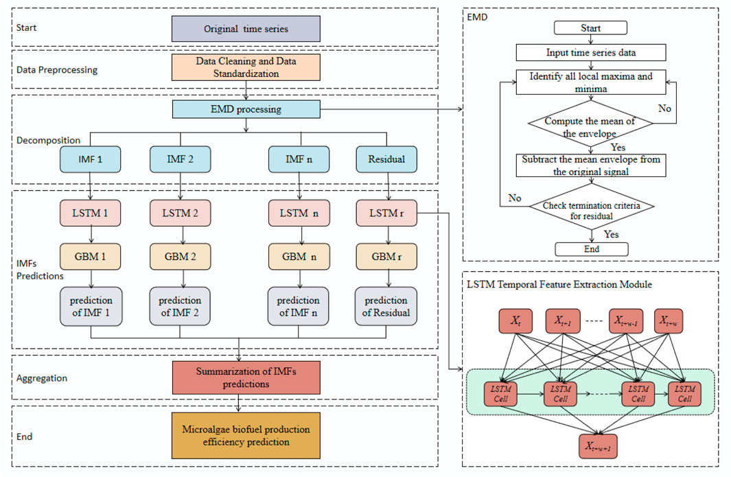
Figure 1. The overall flow chart of ELG model. The figure shows the workflow of the ELG model, which combines EMD, LSTM, and GBM for predicting microalgae biofuel production efficiency. Raw time series data is decomposed into IMFs using EMD, followed by LSTM prediction and GBM optimization. The final prediction is obtained by aggregating all IMF predictions. The right side details the EMD process.

In summary, this ensemble model aims to optimize the prediction of microalgae biofuel production efficiency. The model’s design specifically addresses the nonlinearity and dynamic complexity inherent in biofuel production data, ensuring that predictions are both accurate and reliable. Accurate predictions can aid enterprises in resource planning, process optimization, and ultimately improve production profitability and environmental sustainability. Furthermore, precise predictions offer policymakers a basis for formulating more effective industry support policies and environmental protection measures.

3.2 EMD

Empirical Mode Decomposition (EMD) is an adaptive method for analyzing time series data, aiming to decompose a complex dataset into a series of Intrinsic Mode Functions (IMFs) Shen et al. (2022). Each IMF must satisfy two conditions: within the entire dataset, the number of zero crossings must be equal to or at most differ by one from the number of extrema, and at any point, the local mean (defined by the average of local maxima and minima) must be zero. Thus, EMD systematically extracts fluctuation patterns from time series data, ranging from the fastest-changing oscillations to the slowest-changing trends, with each IMF representing different frequency components of the data Huang et al. (2022).

To provide a rigorous foundation for the Empirical Mode Decomposition (EMD) used in this study, we detail the mathematical framework below. This framework encompasses the initial decomposition process, the iterative extraction of Intrinsic Mode Functions (IMFs), and the criteria for concluding the sifting process. Each equation represents a step in the sequence of operations required to effectively decompose a time series into its component modes.

Initial Residue:

$h_0\left(t\right)=x\left(t\right)$

where $h_0(t)$ represents the initial residue, which is initially set to the input signal $x(t)$.

Identifying Extrema and Envelope Fitting:

$e_{\text{max}}\left(t\right),e_{\text{min}}\left(t\right)=\text{LocalExtrema}\left(h_i\left(t\right)\right)$

${\text{env}}_{\text{upper}}\left(t\right),{\text{env}}_{\text{lower}}\left(t\right)=\text{CubicSpline}\left(e_{\text{max}}\left(t\right),e_{\text{min}}\left(t\right)\right)$

where $e_{\text{max}}(t)$ and $e_{\text{min}}(t)$ are the local maxima and minima of the residue $h_i(t)$, respectively. ${\text{env}}_{\text{upper}}(t)$ and ${\text{env}}_{\text{lower}}(t)$ are the cubic spline interpolations forming the upper and lower envelopes.

Mean Envelope and IMF Extraction:

$m\left(t\right)=\frac{{\text{env}}_{\text{upper}}\left(t\right)+{\text{env}}_{\text{lower}}\left(t\right)}{2}$

$d\left(t\right)=h_i\left(t\right)-m\left(t\right)$

where $m(t)$ is the mean of the upper and lower envelopes, and $d(t)$ is the detail extracted, which is tested to see if it qualifies as an IMF.

IMF Criteria Check and Residue Update:

$h_{i+1}\left(t\right)=h_i\left(t\right)-{\text{IMF}}_i\left(t\right)$

where ${\text{IMF}}_i(t)$ is confirmed if $d(t)$ satisfies the IMF criteria (number of zero crossings and extrema are either equal or differ at most by one, and the mean envelope is zero). Otherwise, $d(t)$ undergoes further sifting.

Stopping Criterion:

$\text{SD}={\displaystyle \sum _{t=0}^T}{\left(\frac{h_i\left(t\right)-h_{i+1}\left(t\right)}{h_i\left(t\right)}\right)}^2$

where SD is the squared difference between consecutive sifting results normalized by the previous residue, $T$ is the total number of observations in the time series, and the process stops when SD becomes smaller than a predetermined threshold, indicating that no more IMFs can be extracted and $h_{i+1}(t)$ becomes the final residue.

In the prediction of microalgae biofuel production efficiency, the introduction of Empirical Mode Decomposition (EMD) is crucial for our ensemble model. By applying EMD, we can effectively extract key periodicities and trends from the raw and complex production data, such as temperature, light intensity, and CO2 concentration logs within the bioreactor. These pieces of information are transformed into a series of more concise and explicit signals (IMFs), each revealing different dynamic variations in the production data. This decomposition allows the subsequent LSTM network to focus more on learning and predicting signals with clear time-dependent characteristics, thereby avoiding potential noise and nonlinear issues that may arise when directly processing raw complex data. Therefore, EMD not only improves the efficiency of data processing but also enhances the accuracy and reliability of the entire predictive model, making predictions of microalgae biofuel production efficiency more precise. Consequently, this aids in optimizing the production process and increasing the final yield.

3.3 LSTM

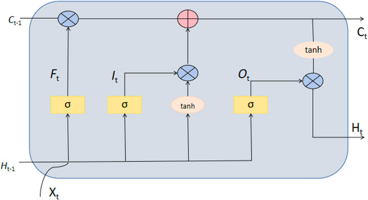
The Long Short-Term Memory (LSTM) network is a specialized type of recurrent neural network (RNN) designed to address the vanishing or exploding gradient problem faced by traditional RNNs when processing long-term dependency information. LSTM, with its unique network architecture comprising gate units (including input gate, forget gate, and output gate), effectively regulates the long-term retention and short-term forgetting of information Meng et al. (2023). The structure diagram of LSTM is shown in Figure 2. This makes LSTM particularly suitable for tasks requiring consideration of long-term dependencies in time series data. Within LSTM units, the forget gate determines which information should be discarded, the input gate controls the importance of new input data, and the output gate decides which information will be used for output Lui et al. (2022). The combined operation of these gates enables LSTM to maintain stability during training, effectively learning and predicting dynamic changes in long time series.

Figure 2

Figure 2. The structure diagram of LSTM.

Here are the five core formulas of LSTM, demonstrating the progressive relationships from input gate, forget gate, output gate to state update:

Input Gate:

$i_t=\sigma \left(W_i\cdot \left[h_{t-1},x_t\right]+b_i\right)$

where $i_t$ is the input gate activation vector, $\sigma$ denotes the sigmoid function, $W_i$ is the weight matrix associated with the input gate, $h_{t-1}$ is the previous hidden state, $x_t$ is the current input vector, and $b_i$ is the input gate bias.

Forget Gate:

$f_t=\sigma \left(W_f\cdot \left[h_{t-1},x_t\right]+b_f\right)$

where $f_t$ is the forget gate activation vector, $\sigma$ denotes the sigmoid function, $W_f$ is the weight matrix associated with the forget gate, and $b_f$ is the forget gate bias.

Cell State Update:

${\tilde{C}}_t=\tanh \left(W_C\cdot \left[h_{t-1},x_t\right]+b_C\right)$

where ${\tilde{C}}_t$ is the candidate cell state, $\tanh$ is the hyperbolic tangent function, $W_C$ is the weight matrix for creating the candidate cell state, and $b_C$ is the bias associated with this update.

Final Cell State:

$C_t=f_t\ast C_{t-1}+i_t\ast {\tilde{C}}_t$

where $C_t$ is the current cell state, $C_{t-1}$ is the previous cell state, $f_t$ is the forget gate’s output, $i_t$ is the input gate’s output, and $\ast$ denotes the element-wise multiplication.

Output Gate and Hidden State Update:

$o_t=\sigma \left(W_o\cdot \left[h_{t-1},x_t\right]+b_o\right)$

$h_t=o_t\ast \tanh \left(C_t\right)$

where $o_t$ is the output gate activation vector, $h_t$ is the current hidden state, $\sigma$ is the sigmoid function, $W_o$ is the weight matrix associated with the output gate, $b_o$ is the output gate bias, and $\tanh (C_t)$ is the hyperbolic tangent function applied to the current cell state.

These formulas demonstrate how LSTM utilizes gate mechanisms at each time step to update its internal state, enabling it to handle time series data with long-term dependencies. The introduction of each gate layer aims to regulate the flow of information, ensuring that the network can make optimal decisions based on both past information and current inputs. The progressive relationships of these formulas clearly illustrate the operation mechanism of LSTM, including how information is stored, updated, and forgotten.

In the microalgae biofuel production efficiency prediction model of this study, the introduction of LSTM is a crucial step. By utilizing LSTM to process the IMFs extracted from EMD, we can accurately capture the time series dynamics in microalgae biofuel production processes. Multiple environmental and production parameters during microalgae cultivation, such as light intensity, temperature, and nutrient supply, exhibit strong temporal correlations, and the historical variations of these parameters are vital for predicting future production efficiency. By memorizing these key patterns in historical data, LSTM enables the model to forecast the growth efficiency of microalgae under specific production conditions, as well as the final biofuel output. This capability not only enhances prediction accuracy but also provides data support for process optimization, enabling operators to adjust production parameters based on forecast results to achieve optimal biofuel yield and quality. Therefore, LSTM not only deepens data processing in our model but also greatly enhances the practicality and effectiveness of predictions.

3.4 GBM

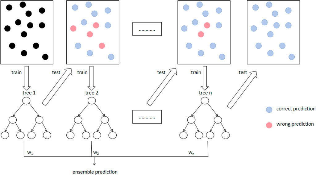
The Gradient Boosting Machine (GBM) is a powerful machine learning algorithm belonging to the ensemble learning methods, specifically based on boosting strategy. GBM iteratively constructs decision tree models, with each new tree attempting to correct the prediction errors of the previous one. At each iteration, GBM applies a new weak learner to further reduce the residuals, which are the differences between the current model’s predictions and the actual values Sunaryono et al. (2022), as illustrated in Figure 3. This process involves computing the gradient of the loss function and then using it to guide the construction of the next decision tree to optimize the overall predictive performance of the model.

Figure 3

Figure 3. A schematic of the GBM process.

For a detailed mathematical exposition of the Gradient Boosting Machine (GBM) as used in your model, we’ll explore five core equations that show the progression of this powerful algorithm.

Loss Function Gradient:

$g_t=-\left[\frac{\partial L\left(y,F_{t-1}\left(x\right)\right)}{\partial F_{t-1}\left(x\right)}\right]$

where $g_t$ is the gradient of the loss function $L$ with respect to the predictions $F_{t-1}(x)$ at iteration $t-1$, $y$ represents the true values, and $x$ denotes the input features.

Residual Computation:

$r_t=y-F_{t-1}\left(x\right)$

where $r_t$ represents the residuals at iteration $t$, computed as the difference between the true values $y$ and the predictions from the previous model $F_{t-1}(x)$.

Weak Learner Contribution:

$h_t\left(x\right)={\mathrm{arg\; min}}_h{\displaystyle \sum _i}L\left(y_i,F_{t-1}\left(x_i\right)+h\left(x_i\right)\right)$

where $h_t(x)$ is the weak learner (e.g., a decision tree) added at iteration $t$ that minimizes the loss when combined with the previous ensemble $F_{t-1}(x)$.

Model Update:

$F_t\left(x\right)=F_{t-1}\left(x\right)+\nu \cdot h_t\left(x\right)$

where $F_t(x)$ is the updated model prediction at iteration $t$, $F_{t-1}(x)$ is the previous model prediction, $h_t(x)$ is the contribution from the new weak learner, and $\nu$ is the learning rate controlling the influence of the new weak learner on the updated model.

Convergence Criterion:

$\text{if\hspace{0.17em}}\left|F_t\left(x\right)-F_{t-1}\left(x\right)\right|<ϵ\text{\hspace{0.17em}then\hspace{0.17em}stop}$

where $ϵ$ is a small threshold value determining when the model’s changes between iterations are negligible, indicating convergence and terminating the algorithm.

In the microalgae biofuel production efficiency prediction model, GBM plays a crucial role. By integrating multiple decision tree models, GBM not only improves prediction accuracy but also enhances the model’s adaptability to complex patterns in production data. In our research, GBM is primarily used to integrate and optimize the data outputs processed through EMD and LSTM. The introduction of GBM significantly enhances the model’s ability to capture nonlinear relationships, which is crucial in the context of microalgae biofuel production, where production efficiency is influenced by various complex environmental and operational parameters. GBM can effectively handle interactions among these variables and finely adjust the model’s response through its optimization algorithm, ensuring high-accuracy predictions under different production conditions. Furthermore, the model results from GBM can provide real-time data support for production process decisions, helping managers adjust production strategies and optimize resource allocation to improve overall production efficiency and economic benefits. In this way, GBM not only enhances the predictive performance of our model but also provides a powerful tool to support the sustainable development of microalgae biofuel production.

4 Experiment

4.1 Datasets

EIA dataset Cilliers et al. (2022): The dataset provided by the U.S. Energy Information Administration (EIA) is a crucial source of information regarding energy production, consumption, and various energy indicators, notably including data on biofuels and renewable energy. These datasets cover multiple aspects ranging from the production of biofuels such as biodiesel and ethanol to the utilization of renewable energy sources. Typically, this information is provided in the form of geographical data (such as state-wise divisions) and time series data (updated on a monthly or yearly basis), making it highly suitable for trend analysis and forecasting. The dataset contains over 10,000 records spanning from 2010 to 2020, with key variables including production volume, energy prices, and environmental factors. The average production volume of biofuels is 500 million gallons per month, with a standard deviation of 50 million gallons. The energy prices range between $2and$4 per gallon, showing seasonal variations. The dataset also exhibits correlations between production and environmental factors, such as temperature and ${\mathrm{C}\mathrm{O}}_2$ emissions, which range from 1 to 3 metric tons per month. Furthermore, the features of the EIA dataset encompass detailed market data and environmental impact data, including prices, demand, supply scenarios for various types of energy, as well as their environmental emissions. In this study, the EIA dataset provides a macro-level market and environmental context for microalgae biofuel production efficiency, aiding researchers in analyzing the positioning of microalgae biofuels within the broader energy market and their environmental benefits.

NREL dataset Present et al. (2024): The dataset provided by the National Renewable Energy Laboratory (NREL) includes extensive information on renewable energy technologies, performance, and costs, with a particular focus on research related to biofuels such as microalgae fuels. This dataset serves as a crucial resource for supporting the development of renewable energy technologies, comprising detailed laboratory test results and field operation data. The NREL dataset includes approximately 5,000 records, focusing on experimental and operational parameters related to microalgae growth, such as light intensity, temperature, and nutrient concentration. The average oil yield in the dataset is 150 L per hectare, with a range of 100–200 L, influenced by factors like nutrient supply and cultivation methods. Standard deviations for these parameters are around 10% of their mean values, reflecting diverse growth conditions. Temporal data spans from 2015 to 2022, and trends indicate an average yearly increase of 5% in biofuel yield. NREL’s data typically offer meticulous parameter records, including microalgae growth conditions, oil yield, and other environmental and operational parameters that affect the efficiency of microalgae biofuel production. These data are highly suitable for analyzing the efficiency and cost of biofuel production, assisting researchers in evaluating the economic viability and environmental sustainability of different production technologies. Through the utilization of the NREL dataset, researchers can gain insight into the specific challenges and potential advantages of microalgae biofuel production, thus providing data support and scientific rationale for improving production efficiency and reducing costs. This is of significant importance for advancing the commercialization and scaling of microalgae biofuel technology.

Figure 4 shows the comparative analysis of biofuel production based on the two datasets. The box plots highlight the variability in biofuel production over the months of 2022 and 2023 for both datasets, providing insights into production trends under different conditions.

Figure 4

Figure 4. Biofuel production trends from 2022 to 2023 based on two datasets. (A) EIA dataset, (B) NREL dataset.

4.2 Experimental details

Step1: Data preprocessing

Data preprocessing is a critical step to ensure the validity and reliability of experimental results. In this study, we performed the following preprocessing steps on the collected time series data:

$•$ Data Cleaning: Data cleaning primarily deals with missing values and outliers. Firstly, we use statistical methods to identify outliers, typically employing the interquartile range (IQR) method, which involves detecting values below the first quartile or above the third quartile by 1.5 times the IQR. For detected outliers, we adopt two strategies: for outliers with a small impact but large in number, we manually review and decide whether to retain or modify them; whereas for outliers with a large impact and large in number, we usually replace them with the median or mean to maintain the overall consistency and reliability of the data. For missing values, we use linear interpolation for imputation.

$•$ Data Standardization: We performed Z-score standardization on the data, achieved by subtracting the mean and dividing by the standard deviation from each feature value. The standardized data has a zero mean and unit variance, helping to eliminate the influence of different scales, balancing the importance of each feature in the model, and accelerating the convergence speed of the model.

$•$ Data Splitting: The dataset is split into training, validation, and testing sets, with proportions of 70%, 15%, and 15%, respectively. This partitioning allows us to train, tune, and evaluate the model on different subsets of data, ensuring the model’s performance on unseen data has good generalization ability.

Through these steps, we effectively enhance the data usability and model training stability, providing a solid data foundation for training deep learning models and subsequent efficiency predictions. These steps ensure that the data we handle not only reflects reality but also meets the requirements of the high-precision prediction models adopted.

Step2:Model training

Model Training Stage is a crucial phase in constructing a high-precision prediction model for microalgae biofuel production efficiency.

$•$ Network Parameter Settings: The settings of network parameters directly influence the model performance. In our ELG model, the parameters for the LSTM layer include setting the number of hidden units to 128, which helps capture long-term dependencies in complex time series data. The number of hidden units (128) was selected based on preliminary experiments and fine-tuning, aiming to balance model complexity and computational efficiency. The learning rate is set to 0.001, which was determined through an extensive grid search combined with cross-validation. This value provided an optimal balance between convergence speed and model stability during training. We utilized the Adam optimizer due to its adaptive learning rate properties, which contribute to rapid and stable convergence. Additionally, to prevent overfitting, we introduce a dropout rate of 0.5 after the LSTM layer, a standard value that was validated through experimentation to ensure robustness across different training conditions.

$•$ Model Architecture Design: Our model architecture is designed as an ensemble model, where EMD is used to preprocess time series data, decomposing it into multiple intrinsic mode functions (IMFs). Subsequently, the LSTM component handles these IMFs, capturing their temporal correlations. Finally, the GBM component further optimizes and predicts the output of LSTM. The entire architecture is designed as a sequence-to-sequence learning framework to handle and predict complex biofuel production efficiency data.

$•$ Model Training Process: During the model training process, we adopted multiple iterations to optimize model parameters in order to improve prediction accuracy. The model underwent several rounds of training on the training set, with a batch size of 32 used in each round to ensure thorough learning while avoiding memory overflow. To prevent overfitting, we implemented early stopping technique, wherein if there was no significant decrease in the loss on the validation set for 20 consecutive rounds of training, the training was automatically stopped. Additionally, after each training stage, we evaluated the model performance on an independent test set to ensure that our model also had good generalization ability on unseen data. Through this approach, we effectively balanced the training efficiency and prediction capability of the model, enabling it to converge rapidly while maintaining high accuracy.

Algorithm 1 outlines the training process of the ELG network, showing initialization, data loading and preprocessing, iterative training with early stopping, and final evaluation.

Algorithm 1.Training ELG Model.

Data: EIA dataset, NREL dataset

Result: Trained ELG model

Initialize: $params\leftarrow \{learning\text{\_}rate=0.01,epochs=100,batch\text{\_}size=32\}$;

Load Data: $data\text{\_}EIA,data\text{\_}NREL\leftarrow$ LoadDatasets();

Preprocess Data: $data\text{\_}processed\leftarrow$ Preprocess($data\text{\_}EIA$, $data\text{\_}NREL$);

Split Data: $train,validate,test\leftarrow$ TrainTestSplit $(data\text{\_}processed)$;

$model\leftarrow$ initializeModel$(params)$;

for $epoch\leftarrow 1$ to$params.epochs$ do

  foreach $batch\leftarrow$ GetBatches$(train,params.batch\text{\_}size)$ do

   $IMFs\leftarrow$ ComputeEMD$(batch)$;

   $predictions\leftarrow model.LSTM\text{\_}forward(IMFs)$;

   $loss\leftarrow$ ComputeLoss$(predictions,batch.labels)$;

   $gradient\leftarrow$ ComputeGradient$(loss)$;

UpdateModel$(model,gradient,params.learning\text{\_}rate)$;

  end

  $validation\text{\_}loss\leftarrow$ Evaluate$(model,validate)$;

  if $validation\text{\_}loss<best\text{\_}loss$ then

   $best\text{\_}loss\leftarrow validation\text{\_}loss$;

   SaveModel$(model)$;

  end

  else if $epoch$ % 10 == 0 then

   if CheckEarlyStopping$(validation\text{\_}loss)$ then

    break

   end

  end

end

$final\text{\_}model\leftarrow$ LoadBestModel();

$test\text{\_}predictions\leftarrow$ Predict$(final\text{\_}model,test)$;

$RMSE\leftarrow$ ComputeRMSE$(test\text{\_}predictions,test.labels)$;

$MAPE\leftarrow$ ComputeMAPE$(test\text{\_}predictions,test.labels)$;

Print: $RMSE,MAPE$;

Step3: Model Evaluation.

$•$ Model Performance Metrics: To assess the performance of the model, several metrics are utilized, each providing insights into different aspects of the model’s predictive accuracy and error characteristics. The primary metrics include Root Mean Square Error (RMSE) for evaluating the average magnitude of the model’s prediction errors, Mean Absolute Error (MAE) for measuring the average magnitude of errors without considering their direction, Coefficient of Determination (R²) for indicating the proportion of variance in the dependent variable predictable from the independent variable(s), and Mean Absolute Percentage Error (MAPE) for offering a normalized measure of errors expressed as a percentage, making it particularly useful for comparing performance across different datasets or models.

$•$ Cross-Validation: To further ensure the robustness and generalizability of the model, a k-fold cross-validation method is implemented. In this approach, the dataset is randomly divided into $k$ equal-sized folds. The model is trained on $k-1$ folds, while the remaining fold is used as a test set to evaluate the model. This process is repeated k times, with each of the k folds used exactly once as the validation data. Typically, $k=10$ is chosen as a balance between training sufficient models and computational efficiency. The average RMSE and MAPE from all k folds are computed to provide an overall measure of model performance. This cross-validation approach helps in mitigating the model’s susceptibility to overfitting and provides a more accurate estimate of how the model is expected to perform on unseen data.

These evaluation steps are crucial for refining the model and ensuring its accuracy and reliability in real-world applications, ultimately supporting effective decision-making in microalgae biofuel production.

The following formulas define the evaluation metrics used in this study:

Root Mean Square Error (RMSE):

$RMSE=\sqrt{\frac{1}{n}{\displaystyle \sum _{i=1}^n}{\left(y_i-{\widehat{y}}_i\right)}^2}$

where $n$ is the number of observations, $y_i$ is the actual value, and ${\widehat{y}}_i$ is the predicted value.

Mean Absolute Error (MAE):

$MAE=\frac{1}{n}{\displaystyle \sum _{i=1}^n}|y_i-{\widehat{y}}_i|$

where $n$ is the number of observations, $y_i$ is the actual value, and ${\widehat{y}}_i$ is the predicted value.

Coefficient of Determination (${\mathrm{R}}^2$):

$R^2=1-\frac{\sum _{i=1}^n{\left(y_i-{\widehat{y}}_i\right)}^2}{\sum _{i=1}^n{\left(y_i-\bar{y}\right)}^2}$

where $n$ is the number of observations, $y_i$ is the actual value, ${\widehat{y}}_i$ is the predicted value, and $\bar{y}$ is the mean of the actual values.

Mean Absolute Percentage Error (MAPE):

$MAPE=\frac{1}{n}{\displaystyle \sum _{i=1}^n}\left|\frac{y_i-{\widehat{y}}_i}{y_i}\right|\times 100$

where $n$ is the number of observations, $y_i$ is the actual value, and ${\widehat{y}}_i$ is the predicted value.

4.3 Experimental results and analysis

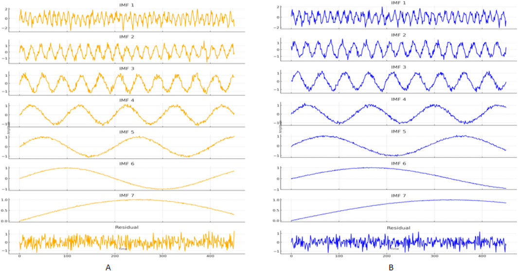
Figure 5 shows the EMD decomposition results for the EIA dataset (A) and the NREL dataset (B). Each dataset’s decomposition includes seven Intrinsic Mode Functions (IMF 1 to IMF 7) and one residual. The IMFs represent different frequency components from high to low, while the residual captures the long-term trend. Each subplot illustrates the variations of different frequency components and the residual part within the dataset.

Figure 5

Figure 5. EMD decomposition results for the EIA dataset (A) and the NREL dataset (B).

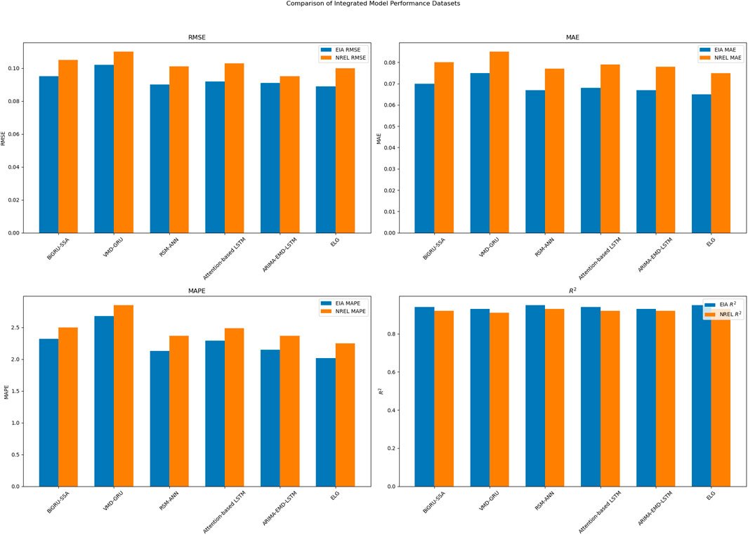
As shown in Table 1, we compared the predictive performance of various ensemble models on the EIA and NREL datasets. Our proposed ELG model excelled across all metrics, demonstrating its superiority in predicting the efficiency of microalgae biofuel production. In the EIA dataset, the ELG model achieved an RMSE of 0.089, MAE of 0.065, MAPE of 2.01%, and $R^2$ of 0.95. In comparison, the RSM-ANN model had an RMSE of 0.09, MAE of 0.067, MAPE of 2.13%, and $R^2$ of 0.95. Although both models had the same $R^2$, the ELG model outperformed in terms of RMSE and MAPE, reducing them by 0.001 and 0.12 percentage points, respectively. This indicates that the ELG model is more effective in minimizing both absolute and relative errors. Compared to other state-of-the-art models such as the BiGRU-SSA and Attention-based LSTM, the ELG model also shows significant improvements. For instance, the BiGRU-SSA model had an RMSE of 0.095 and MAPE of 2.32% on the EIA dataset, while the ELG model achieved an RMSE of 0.089 and MAPE of 2.01%, representing improvements of 6.3% and 13.4%, respectively. Similarly, on the NREL dataset, the ELG model outperformed the BiGRU-SSA model by 4.8% in RMSE and 11.6% in MAPE. These comparisons clearly demonstrate the ELG model’s robustness and effectiveness in improving prediction accuracy over existing models. For the NREL dataset, the ELG model achieved an RMSE of 0.1, MAE of 0.075, MAPE of 2.21%, and $R^2$ of 0.93. In contrast, the RSM-ANN model had an RMSE of 0.101, MAE of 0.077, MAPE of 2.37%, and $R^2$ of 0.93. Despite the same $R^2$, the ELG model again outperformed with better RMSE, MAE, and MAPE values, reducing them by 0.001, 0.002, and 0.16 percentage points, respectively. These results not only highlight the superior performance of the ELG model but also position it as a strong competitor among the latest models in the literature, further validating its practical applicability. Additionally, the BiGRU-SSA model had an RMSE of 0.095 and MAPE of 2.32% on the EIA dataset, while the ELG model achieved an RMSE of 0.089 and MAPE of 2.01%, improving by approximately 6.3% and 13.4%, respectively. On the NREL dataset, the BiGRU-SSA model’s RMSE and MAPE were 0.105% and 2.5%, respectively, whereas the ELG model achieved 0.1% and 2.21%, improving by 4.8% and 11.6%, respectively. Figure 6 visualizes the table’s data, allowing readers to more intuitively understand the performance differences of each model across the datasets. These visualizations clearly highlight the advantages of our proposed ELG model in various metrics, further validating its effectiveness and reliability in practical applications.

Table 1

Table 1. Comparison of integrated model performance datasets.

Figure 6

Figure 6. Comparison of integrated model performance datasets.

As shown in Table 2, we compared the performance of various ensemble models on the EIA and NREL datasets, displaying each model’s number of parameters, FLOPs (Floating Point Operations), inference time, and training time. Our proposed ELG model demonstrates significant advantages in all these aspects. In the EIA dataset, the ELG model has 130.74 M parameters, 175.18G FLOPs, an inference time of 130.81 ms, and a training time of 229.51 s. In contrast, the BiGRU-SSA model has 289.13 M parameters, 323.25G FLOPs, an inference time of 279.64 ms, and a training time of 318.91 s. The ELG model reduces the number of parameters, FLOPs, inference time, and training time by 158.39 M, 148.07G FLOPs, 148.83 ms, and 89.4 s, respectively, demonstrating its computational efficiency. In the NREL dataset, the ELG model has 232.19 M parameters, 217.45G FLOPs, an inference time of 206.98 ms, and a training time of 214.28 s. In comparison, the BiGRU-SSA model has 235.51 M parameters, 300.67G FLOPs, an inference time of 357.15 ms, and a training time of 590.01 s. Here, the ELG model outperforms by reducing these metrics by 3.32 M parameters, 83.22G FLOPs, 150.17 ms, and 375.73 s, respectively. Compared to other models such as VMD-GRU and RSM-ANN, the ELG model also shows superior performance on both the EIA and NREL datasets, significantly reducing computational resources required. These results underscore the ELG model’s ability to deliver high performance with lower computational cost. Figure 7 visualizes the table contents, allowing readers to more intuitively understand the performance differences of each model across the datasets. The visual results highlight the computational and performance advantages of our proposed ELG model, validating its effectiveness and reliability in practical applications.

Table 2

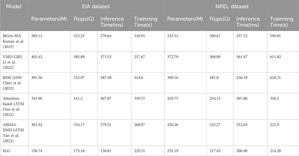
Table 2. Comparison of model performance on EIA and NREL datasets: Parameters, flops, inference time, and training time.

Figure 7

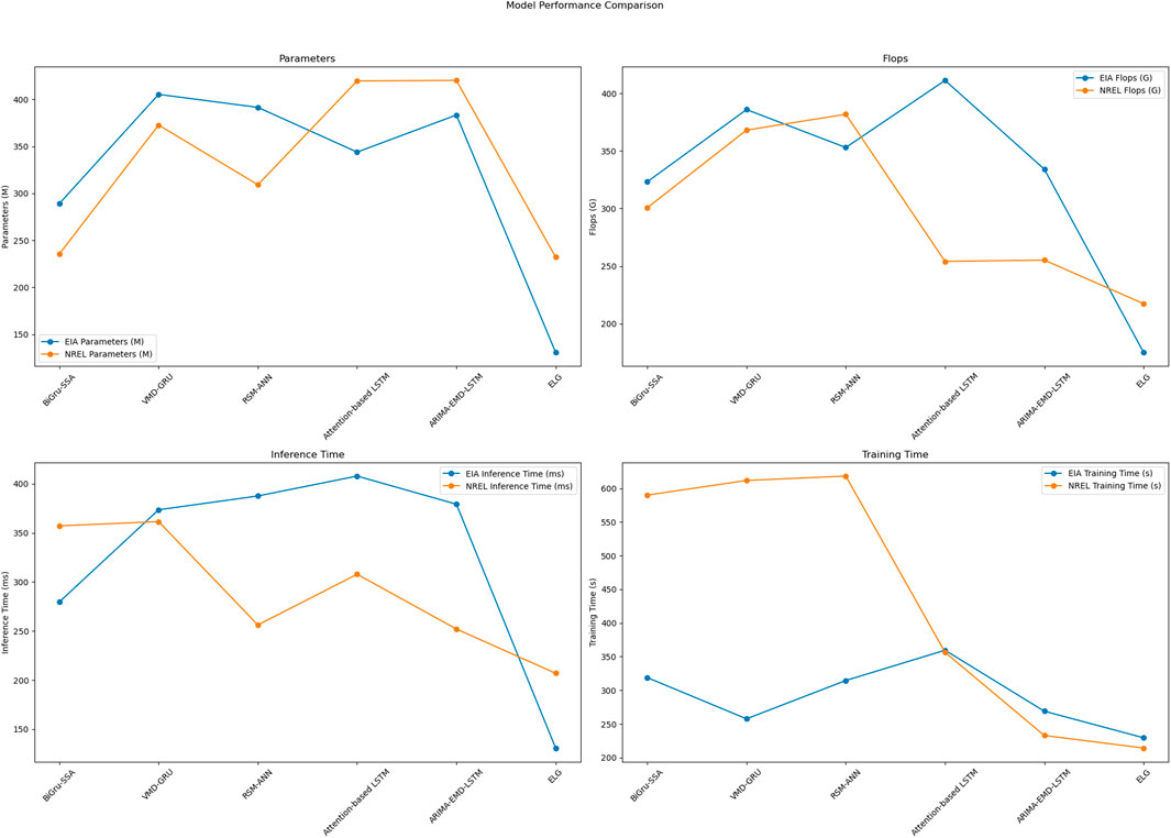
Figure 7. Comparison of model performance on EIA and NREL datasets: Parameters, Flops, inference time, and training time.

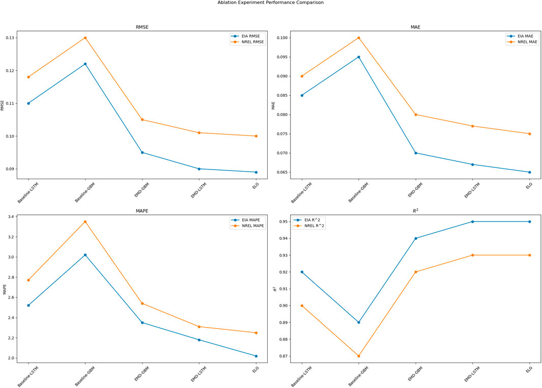
As shown in Table 3, we conducted ablation experiments to compare the performance of different models on the EIA and NREL datasets, presenting each model’s RMSE, MAE, MAPE, and $R^2$ metrics. By progressively removing components from the model, we analyzed the contribution of each component to the overall performance. The results show that our complete ELG model excels in all metrics, highlighting the importance of each component in enhancing model performance. In the EIA dataset, the complete ELG model achieved an RMSE of 0.089, MAE of 0.065, MAPE of 2.02%, and $R^2$ of 0.95. In contrast, the Baseline-LSTM model, which excludes EMD, had an RMSE of 0.11, MAE of 0.085, MAPE of 2.52%, and $R^2$ of 0.92. The Baseline-GBM model, which excludes LSTM, had an RMSE of 0.122, MAE of 0.095, MAPE of 3.02%, and $R^2$ of 0.89. This indicates that the combination of EMD and LSTM significantly enhances the model’s predictive performance by reducing prediction errors and increasing the $R^2$ value. In the NREL dataset, the complete ELG model achieved an RMSE of 0.1, MAE of 0.075, MAPE of 2.25%, and $R^2$ of 0.93. In comparison, the Baseline-LSTM model had an RMSE of 0.118, MAE of 0.09, MAPE of 2.77%, and $R^2$ of 0.9, while the Baseline-GBM model had an RMSE of 0.13, MAE of 0.1, MAPE of 3.35%, and $R^2$ of 0.87. These results further validate the superiority of the complete model, especially in handling complex time series data. Further ablation experiments show that models using only EMD and GBM (EMD-GBM) and those using only EMD and LSTM (EMD-LSTM) also underperform compared to the complete ELG model. For instance, in the EIA dataset, the EMD-GBM model achieved an RMSE of 0.095, MAE of 0.07, MAPE of 2.35%, and $R^2$ of 0.94, while the EMD-LSTM model had an RMSE of 0.09, MAE of 0.067, MAPE of 2.18%, and $R^2$ of 0.95. The ELG model outperformed these models, particularly in MAE and MAPE metrics. In the NREL dataset, the EMD-GBM model had an RMSE of 0.105, MAE of 0.08, MAPE of 2.54%, and $R^2$ of 0.92, while the EMD-LSTM model achieved an RMSE of 0.101, MAE of 0.077, MAPE of 2.31%, and $R^2$ of 0.93. The complete ELG model performed better in all these metrics, demonstrating its strong performance on diverse and complex datasets.

Table 3

Table 3. Ablation experiment performance data comparison.

These ablation experiment results indicate that the combination of EMD, LSTM, and GBM significantly enhances model performance. The components work synergistically to handle temporal dependencies and nonlinear relationships in the data, significantly improving predictive accuracy and stability. Figure 8 visualizes the table’s content, allowing readers to intuitively understand the performance differences of each model across the datasets. These visual results clearly highlight the advantages of our proposed ELG model in various metrics, further validating its effectiveness and reliability in practical applications.

Figure 8

Figure 8. Ablation experiment performance data comparison.

5 Conclusion

In this study, we developed and evaluated an innovative ELG model designed to predict the efficiency of microalgae biofuel production. Our approach integrates Empirical Mode Decomposition (EMD), Long Short-Term Memory (LSTM) networks, and Gradient Boosting Machine (GBM) to harness the strengths of each method. We conducted extensive experiments on the EIA and NREL datasets, comparing the ELG model’s performance with several baseline models through comprehensive metrics such as RMSE, MAE, MAPE, and $R^2$. The results demonstrated that our ELG model significantly outperforms baseline models, effectively reducing prediction errors and increasing the $R^2$ values. The practical implications of our findings suggest that the ELG model can directly improve biofuel production processes by providing more accurate efficiency predictions. This enhanced accuracy enables better resource allocation and cost reduction, ultimately leading to more efficient biofuel production. Additionally, the model’s robustness across varying conditions indicates its potential utility in other renewable energy applications, where similar challenges in prediction accuracy and resource management exist. Despite the promising results, our model has some limitations. Firstly, the ELG model’s complexity and computational requirements, while optimized compared to individual baseline models, remain substantial. The high computational cost associated with training and inference could limit its applicability in scenarios with limited computational resources or real-time requirements. Secondly, the model’s performance may vary with different datasets and environmental conditions. While it performs well on the EIA and NREL datasets, its generalizability to other datasets or production conditions has yet to be fully tested. This variability underscores the need for further validation across diverse datasets and conditions to ensure the model’s robustness and adaptability.

Looking ahead, several potential directions for future research can be pursued. One important direction is to further optimize the model to reduce computational complexity while maintaining high performance. Techniques such as model pruning, quantization, or exploring more efficient architectures could be valuable in achieving this goal. Additionally, expanding the dataset by incorporating more diverse and extensive data sources would enhance the model’s generalizability and robustness, making it more applicable across various conditions. Integrating additional environmental and operational parameters into the model could also provide a more comprehensive understanding of the factors influencing biofuel production efficiency. Finally, testing the ELG model in real-world biofuel production environments would be crucial for validating its practical utility and identifying areas for refinement. These efforts would collectively contribute to advancing the predictive modeling of microalgae biofuel production efficiency, supporting the broader goal of enhancing biofuel production processes and sustainability.

Data availability statement

The original contributions presented in the study are included in the article/supplementary material, further inquiries can be directed to the corresponding author.

Author contributions

YW: Data curation, Formal Analysis, Methodology, Resources, Validation, Visualization, Writing–original draft. CZ: Conceptualization, Investigation, Project administration, Software, Supervision, Writing–review and editing.

Funding

The author(s) declare that no financial support was received for the research, authorship, and/or publication of this article.

Conflict of interest

The authors declare that the research was conducted in the absence of any commercial or financial relationships that could be construed as a potential conflict of interest.

Publisher’s note

All claims expressed in this article are solely those of the authors and do not necessarily represent those of their affiliated organizations, or those of the publisher, the editors and the reviewers. Any product that may be evaluated in this article, or claim that may be made by its manufacturer, is not guaranteed or endorsed by the publisher.

References

Bijitha, C., and Nath, H. V. (2022). On the effectiveness of image processing based malware detection techniques. Cybern. Syst. 53, 615–640. doi:10.1080/01969722.2021.2020471

CrossRef Full Text | Google Scholar

Chen, H., Wu, H., Kan, T., Zhang, J., and Li, H. (2023). Low-carbon economic dispatch of integrated energy system containing electric hydrogen production based on vmd-gru short-term wind power prediction. Int. J. Electr. Power and Energy Syst. 154, 109420. doi:10.1016/j.ijepes.2023.109420

CrossRef Full Text | Google Scholar

Chong, J. W. R., Khoo, K. S., Chew, K. W., Ting, H.-Y., Iwamoto, K., Ruan, R., et al. (2024). Artificial intelligence-driven microalgae autotrophic batch cultivation: a comparative study of machine and deep learning-based image classification models. Algal Res. 79, 103400. doi:10.1016/j.algal.2024.103400

CrossRef Full Text | Google Scholar

Cilliers, D., Retief, F., Bond, A., Roos, C., and Alberts, R. (2022). The validity of spatial data-based eia screening decisions. Environ. Impact Assess. Rev. 93, 106729. doi:10.1016/j.eiar.2021.106729

CrossRef Full Text | Google Scholar

Dong, Y., Li, J., Liu, Z., Niu, X., and Wang, J. (2022). Ensemble wind speed forecasting system based on optimal model adaptive selection strategy: case study in China. Sustain. Energy Technol. Assessments 53, 102535. doi:10.1016/j.seta.2022.102535

CrossRef Full Text | Google Scholar

Dong, Y., Sun, Y., Liu, Z., Du, Z., and Wang, J. (2024). Predicting dissolved oxygen level using young’s double-slit experiment optimizer-based weighting model. J. Environ. Manag. 351, 119807. doi:10.1016/j.jenvman.2023.119807

CrossRef Full Text | Google Scholar

Dong, Y., Zhang, L., Liu, Z., and Wang, J. (2019). Integrated forecasting method for wind energy management: a case study in China. Processes 8, 35. doi:10.3390/pr8010035

CrossRef Full Text | Google Scholar

Drożdż, W., Bilan, Y., Rabe, M., Streimikiene, D., and Pilecki, B. (2022). Optimizing biomass energy production at the municipal level to move to low-carbon energy. Sustain. Cities Soc. 76, 103417. doi:10.1016/j.scs.2021.103417

CrossRef Full Text | Google Scholar

Dubey, A. K., Kumar, A., Ramirez, I. S., and Marquez, F. P. G. (2022). “A review of intelligent systems for the prediction of wind energy using machine learning,” in International Conference on Management Science and Engineering Management (Springer), 476–491.

CrossRef Full Text | Google Scholar

Elsaraiti, M., and Merabet, A. (2022). Solar power forecasting using deep learning techniques. IEEE access 10, 31692–31698. doi:10.1109/access.2022.3160484

CrossRef Full Text | Google Scholar

Gao, T., Wang, C., Zheng, J., Wu, G., Ning, X., Bai, X., et al. (2023). A smoothing group lasso based interval type-2 fuzzy neural network for simultaneous feature selection and system identification. Knowledge-Based Syst. 280, 111028. doi:10.1016/j.knosys.2023.111028

CrossRef Full Text | Google Scholar

Hoang, A. T., Nguyen, X. P., Duong, X. Q., Ağbulut, Ü., Len, C., Nguyen, P. Q. P., et al. (2023). Steam explosion as sustainable biomass pretreatment technique for biofuel production: characteristics and challenges. Bioresour. Technol. 385, 129398. doi:10.1016/j.biortech.2023.129398

PubMed Abstract | CrossRef Full Text | Google Scholar

Huang, J., Wang, J., Huang, Z., Liu, T., and Li, H. (2023). Photothermal technique-enabled ambient production of microalgae biodiesel: mechanism and life cycle assessment. Bioresour. Technol. 369, 128390. doi:10.1016/j.biortech.2022.128390

PubMed Abstract | CrossRef Full Text | Google Scholar

Huang, Y., Hasan, N., Deng, C., and Bao, Y. (2022). Multivariate empirical mode decomposition based hybrid model for day-ahead peak load forecasting. Energy 239, 122245. doi:10.1016/j.energy.2021.122245

CrossRef Full Text | Google Scholar

Jiang, P., Liu, Z., Zhang, L., and Wang, J. (2022). Advanced traffic congestion early warning system based on traffic flow forecasting and extenics evaluation. Appl. Soft Comput. 118, 108544. doi:10.1016/j.asoc.2022.108544

CrossRef Full Text | Google Scholar

Kumar, I., Tripathi, B. K., and Singh, A. (2023). Attention-based lstm network-assisted time series forecasting models for petroleum production. Eng. Appl. Artif. Intell. 123, 106440. doi:10.1016/j.engappai.2023.106440

CrossRef Full Text | Google Scholar

Li, X., Ma, X., Xiao, F., Xiao, C., Wang, F., and Zhang, S. (2022). Time-series production forecasting method based on the integration of bidirectional gated recurrent unit (bi-gru) network and sparrow search algorithm (ssa). J. Petroleum Sci. Eng. 208, 109309. doi:10.1016/j.petrol.2021.109309

CrossRef Full Text | Google Scholar

Liu, Y., Meenakshi, V., Karthikeyan, L., Maroušek, J., Krishnamoorthy, N., Sekar, M., et al. (2022). Machine learning based predictive modelling of micro gas turbine engine fuelled with microalgae blends on using lstm networks: an experimental approach. Fuel 322, 124183. doi:10.1016/j.fuel.2022.124183

CrossRef Full Text | Google Scholar

Lui, C. F., Liu, Y., and Xie, M. (2022). A supervised bidirectional long short-term memory network for data-driven dynamic soft sensor modeling. IEEE Trans. Instrum. Meas. 71, 1–13. doi:10.1109/tim.2022.3152856

CrossRef Full Text | Google Scholar

Ma, G., and Chen, X. (2024). From financial power to financial powerhouse: international comparison and China’s approach. J. Xi’an Univ. Finance Econ. 37, 46–59.

Google Scholar

Ma, Y., Liu, S., Wang, Y., and Wang, Y. (2023). Processing wet microalgae for direct biodiesel production: optimization of the two-stage process assisted by radio frequency heating. Int. J. Green Energy 20, 477–485. doi:10.1080/15435075.2022.2070023

CrossRef Full Text | Google Scholar

Maya, M., Yu, W., and Telesca, L. (2022). Multi-step forecasting of earthquake magnitude using meta-learning based neural networks. Cybern. Syst. 53, 563–580. doi:10.1080/01969722.2021.1989170

CrossRef Full Text | Google Scholar

Meng, H., Geng, M., and Han, T. (2023). Long short-term memory network with bayesian optimization for health prognostics of lithium-ion batteries based on partial incremental capacity analysis. Reliab. Eng. and Syst. Saf. 236, 109288. doi:10.1016/j.ress.2023.109288

CrossRef Full Text | Google Scholar

Onu, C. E., Nweke, C. N., and Nwabanne, J. T. (2022). Modeling of thermo-chemical pretreatment of yam peel substrate for biogas energy production: Rsm, ann, and anfis comparative approach. Appl. Surf. Sci. Adv. 11, 100299. doi:10.1016/j.apsadv.2022.100299

CrossRef Full Text | Google Scholar

Present, E., White, P. R., Harris, C., Adhikari, R., Lou, Y., Liu, L., et al. (2024). “ResStock dataset 2024.1 documentation. Tech. Rep,”. Golden, CO (United States): National Renewable Energy Laboratory NREL.

Google Scholar

Sathya, A. B., Thirunavukkarasu, A., Nithya, R., Nandan, A., Sakthishobana, K., Kola, A. K., et al. (2023). Microalgal biofuel production: potential challenges and prospective research. Fuel 332, 126199. doi:10.1016/j.fuel.2022.126199

CrossRef Full Text | Google Scholar

Sharma, V., Tsai, M.-L., Chen, C.-W., Sun, P.-P., Nargotra, P., and Dong, C.-D. (2023). Advances in machine learning technology for sustainable biofuel production systems in lignocellulosic biorefineries. Sci. Total Environ. 886, 163972. doi:10.1016/j.scitotenv.2023.163972

PubMed Abstract | CrossRef Full Text | Google Scholar

Shen, J., Zhang, Y., Liang, H., Zhao, Z., Dong, Q., Qian, K., et al. (2022). Exploring the intrinsic features of eeg signals via empirical mode decomposition for depression recognition. IEEE Trans. Neural Syst. Rehabilitation Eng. 31, 356–365. doi:10.1109/tnsre.2022.3221962

CrossRef Full Text | Google Scholar

Sonmez, M. E., Eczacıoglu, N., Gumuş, N. E., Aslan, M. F., Sabanci, K., and Aşikkutlu, B. (2022). Convolutional neural network-support vector machine based approach for classification of cyanobacteria and chlorophyta microalgae groups. Algal Res. 61, 102568. doi:10.1016/j.algal.2021.102568

CrossRef Full Text | Google Scholar

Subhash, G. V., Rajvanshi, M., Kumar, G. R. K., Sagaram, U. S., Prasad, V., Govindachary, S., et al. (2022). Challenges in microalgal biofuel production: a perspective on techno economic feasibility under biorefinery stratagem. Bioresour. Technol. 343, 126155. doi:10.1016/j.biortech.2021.126155

PubMed Abstract | CrossRef Full Text | Google Scholar

Sultana, N., Hossain, S. Z., Abusaad, M., Alanbar, N., Senan, Y., and Razzak, S. (2022). Prediction of biodiesel production from microalgal oil using bayesian optimization algorithm-based machine learning approaches. Fuel 309, 122184. doi:10.1016/j.fuel.2021.122184

CrossRef Full Text | Google Scholar

Sun, Y., Ding, J., Liu, Z., and Wang, J. (2023). Combined forecasting tool for renewable energy management in sustainable supply chains. Comput. and Industrial Eng. 179, 109237. doi:10.1016/j.cie.2023.109237

CrossRef Full Text | Google Scholar

Sunaryono, D., Sarno, R., and Siswantoro, J. (2022). Gradient boosting machines fusion for automatic epilepsy detection from eeg signals based on wavelet features. J. King Saud University-Computer Inf. Sci. 34, 9591–9607. doi:10.1016/j.jksuci.2021.11.015

CrossRef Full Text | Google Scholar

Svetunkov, I., Kourentzes, N., and Ord, J. K. (2022). Complex exponential smoothing. Nav. Res. Logist. (NRL) 69, 1108–1123. doi:10.1002/nav.22074

CrossRef Full Text | Google Scholar

Syed, T., Krujatz, F., Ihadjadene, Y., Mühlstädt, G., Hamedi, H., Mädler, J., et al. (2024). A review on machine learning approaches for microalgae cultivation systems. Comput. Biol. Med. 172, 108248. doi:10.1016/j.compbiomed.2024.108248

PubMed Abstract | CrossRef Full Text | Google Scholar

Tian, S., Li, W., Ning, X., Ran, H., Qin, H., and Tiwari, P. (2023). Continuous transfer of neural network representational similarity for incremental learning. Neurocomputing 545, 126300. doi:10.1016/j.neucom.2023.126300

CrossRef Full Text | Google Scholar

Wang, J., Li, F., An, Y., Zhang, X., and Sun, H. (2024). Towards robust lidar-camera fusion in bev space via mutual deformable attention and temporal aggregation. IEEE Trans. Circuits Syst. Video Technol., 1–1doi. doi:10.1109/TCSVT.2024.3366664

CrossRef Full Text | Google Scholar

Yan, Y., Wang, X., Ren, F., Shao, Z., and Tian, C. (2022). Wind speed prediction using a hybrid model of eemd and lstm considering seasonal features. Energy Rep. 8, 8965–8980. doi:10.1016/j.egyr.2022.07.007

CrossRef Full Text | Google Scholar

Yao, Y., and Liu, Z. (2024). The new development concept helps accelerate the formation of new quality productivity: theoretical logic and implementation paths. J. Xi’an Univ. Finance Econ. 37, 3–14.

Google Scholar

Yu, L., Liang, S., Chen, R., and Lai, K. K. (2022). Predicting monthly biofuel production using a hybrid ensemble forecasting methodology. Int. J. Forecast. 38, 3–20. doi:10.1016/j.ijforecast.2019.08.014

CrossRef Full Text | Google Scholar