Water resource asset assessment and financial decision support based on multi-source remote sensing data

Introduction: Assessing water resource assets in dynamic environmental conditions presents significant scientific and operational challenges. Remote sensing data are often multi-source, high-dimensional, and temporally inconsistent, making it difficult to construct models that are both accurate and generalizable. Moreover, existing financial decision support systems struggle with integrating environmental variability, spatiotemporal noise, and the real-time interpretability required for practical deployment. Addressing these issues requires a fundamentally new approach that unifies data fusion, spatiotemporal modeling, and financial risk assessment into a cohesive system.

Methods: This study introduces the Contextual Multi-source Decision Network (CMDN), a hybrid deep learning framework that incorporates adaptive volatility modeling, multi-scale temporal analysis, and cross-modal attention mechanisms. By doing so, we aim to bridge the gap between remote sensing technologies and financial planning, enabling more accurate, transparent, and timely decision-making in water resource management.

Results: Extensive experiments on GRACE, MODIS, ERA5-Land, and SEN12MS datasets demonstrate that CMDN reduces RMSE by up to 12.3% and improves R² scores by 2%–4% compared to state-of-the-art baselines.

Discussion: The study identifies two key limitations. The complexity and computational intensity of integrating multi-source data and machine learning models may restrict accessibility, especially in regions with limited technological resources. These results confirm its value as a scalable and actionable tool for sustainable resource management under uncertain and evolving environmental conditions.

1 Introduction

The assessment of water resource assets plays a critical role in ensuring sustainable management and efficient utilization of this vital resource, especially in the context of growing global water scarcity Zhou et al. (2020). Traditional methods often face challenges in capturing the spatial and temporal complexities of water resources, limiting their ability to inform effective financial and policy decisions Zeng et al. (2022). The advent of multi-source remote sensing technologies has revolutionized water resource monitoring, offering comprehensive, high-resolution data on surface water, groundwater, and environmental factors Liu et al. (2023). By integrating these data sources into robust financial decision support frameworks, stakeholders can make informed choices that balance environmental conservation with economic priorities Zhang and Yan (2023). This research seeks to bridge the gap between advanced remote sensing techniques and practical financial decision-making, providing a scalable and data-driven approach to water resource management Wu et al. (2020).

Initial efforts to assess water resources for financial decision-making relied on symbolic AI and rule-based systems, which integrated knowledge representation with structured hydrological models Jin et al. (2023). These methods used static datasets from limited ground-based measurements and historical records, combined with expert rules to estimate water availability and predict economic outcomes Chen et al. (2023). While effective in specific, localized contexts, these approaches suffered from significant limitations, including their inability to process real-time or large-scale data Das et al. (2023). The lack of integration with dynamic environmental factors further reduced their relevance in rapidly changing conditions Li et al. (2023). The financial decision-making process remained constrained by incomplete and outdated assessments, necessitating the adoption of more adaptable and data-rich methodologies Yi et al. (2023).

While technical progress in remote sensing and predictive modeling has significantly enhanced the granularity and accuracy of water resource assessments, a critical challenge remains in aligning these sophisticated tools with the practical needs of decision-makers. Government agencies and local water managers often operate under resource constraints and require decision support systems that are not only scientifically sound but also easy to interpret and implement. Complex models, although powerful, can hinder operational use if their outputs are not translated into user-friendly formats. Furthermore, the socio-economic context and local governance structures play a decisive role in determining whether a technical solution can be effectively adopted. Variability in policy priorities, regulatory frameworks, and institutional capacities across regions means that even the most advanced models may see limited real-world application unless they are adapted to these local conditions. Therefore, bridging this gap between technical rigor and practical utility is essential for achieving meaningful outcomes in water resource management.

To overcome the shortcomings of traditional approaches, data-driven methodologies leveraging machine learning and statistical modeling were introduced Ekambaram et al. (2023). These methods utilized larger datasets, including early remote sensing data, to create predictive models for water resource availability and financial impacts Kim et al. (2022). Machine learning algorithms, such as regression models and decision trees, were employed to identify patterns in hydrological and economic data He et al. (2023). Multi-source remote sensing data—captured from satellites and aerial surveys—enhanced these models by providing more accurate and expansive environmental insights Woo et al. (2022). Despite these advancements, data-driven approaches often struggled with integrating diverse and heterogeneous datasets Liu et al. (2022). Their predictive capabilities were limited by the quality of the training data, which frequently failed to account for long-term environmental and financial trends.

The integration of deep learning with multi-source remote sensing data has marked a significant breakthrough in water resource assessment and financial decision support Rasul et al. (2021). Deep learning models, particularly convolutional neural networks (CNNs) and recurrent neural networks (RNNs), have demonstrated exceptional performance in processing high-dimensional remote sensing data and identifying complex spatiotemporal patterns Lim and Zohren (2020). Multi-source data, including optical, radar, and thermal imagery, can now be fused to provide a holistic view of water resources, capturing surface water dynamics, groundwater variations, and precipitation patterns Shao et al. (2022). Challenges remain in terms of the computational cost, the need for extensive labeled datasets, and the integration of socioeconomic factors into decision-making frameworks Challu et al. (2022).

To address these pressing challenges, we propose the Contextual Multi-source Decision Network (CMDN), a novel hybrid forecasting framework that integrates volatility-aware attention, multi-scale temporal encoding, and financial interpretability into a unified system. CMDN departs from conventional models by explicitly modeling uncertainty, decomposing temporal-spatial interactions through dual-branch encoders, and introducing risk-adjusted loss functions. These design elements collectively enable the model to outperform existing methods in both accuracy and decision robustness. This work represents the first attempt to fuse multi-source remote sensing with financial volatility modeling in a fully end-to-end trainable architecture.

$•$ Combines multi-source remote sensing data with domain-specific financial models, ensuring comprehensive and actionable insights.

$•$ Offers a lightweight framework suitable for diverse geographic regions, reducing computational costs while maintaining high accuracy.

$•$ Initial tests demonstrate improved accuracy in asset valuation and financial decision support, enhancing stakeholder confidence and resource management outcomes.

2 Related work

2.1 Multi-source remote sensing for water resource monitoring

The integration of multi-source remote sensing data has significantly advanced the monitoring and assessment of water resources Cao et al. (2020). Optical, thermal, and radar remote sensing provide complementary datasets that enable a comprehensive understanding of surface water dynamics, groundwater availability, and watershed health Xue and Salim (2022). High-resolution optical imagery from satellites such as Landsat and Sentinel is widely used for delineating water bodies, while thermal sensors help assess evaporation rates and temperature-induced stress on aquatic ecosystems Jin et al. (2022). Synthetic Aperture Radar (SAR) data, with its all-weather capability, plays a critical role in detecting subsurface water and monitoring flood events Mi et al. (2024). Combining these diverse data streams through data fusion techniques enhances the accuracy and temporal resolution of water resource monitoring. Machine learning algorithms, including deep learning models, are increasingly employed to automate the classification and segmentation of water-related features from these datasets. Challenges such as data heterogeneity, sensor calibration, and the high computational cost of processing large datasets remain critical barriers. Despite these challenges, multi-source remote sensing offers unparalleled opportunities for assessing water resources with precision and scalability.

2.2 Valuation of water resources as assets

Water resources are increasingly recognized as critical economic assets, requiring robust frameworks for their valuation to inform financial decision-making Ye et al. (2022). The concept of water as a quantifiable asset involves the integration of hydrological, ecological, and socio-economic factors to estimate its value accurately Hajirahimi and Khashei (2022). Multi-source remote sensing data plays a pivotal role in quantifying key parameters such as water availability, quality, and usage patterns Wang et al. (2022). By linking this information with economic valuation models, policymakers can assess the sustainability and economic contribution of water resources to various sectors, including agriculture, energy, and urban development Cheng et al. (2022). Techniques such as water accounting and satellite-based measurements of water volume changes in reservoirs and aquifers provide actionable insights Pukanská et al. (2024). Research has also explored the use of remote sensing-derived indices, such as the Normalized Difference Water Index (NDWI) and Surface Water Supply Index (SWSI), for resource valuation. Although there is growing progress in integrating remote sensing into water valuation, challenges such as translating biophysical data into economic metrics and addressing uncertainties in remote sensing measurements require further exploration.

Recent advances in water economics highlight the importance of incorporating market-based and non-market valuation methods in water management systems Griffin (2006). Seminal works by Rogers et al. (1998) and Griffin (2006) emphasize that water should be treated as an economic good, with valuation approaches that include opportunity cost, replacement cost, and willingness-to-pay metrics Rogers et al. (1998). Global institutions such as the World Bank (2020) and FAO (2012) have published policy frameworks advocating volumetric pricing, tiered tariffs, and economic modeling tools to balance efficiency, sustainability, and affordability Bank (2020). Integrating such economic perspectives into hydrological modeling enhances the interpretability and actionability of AI-generated outputs in water-stressed regions FAO (2012).

2.3 Financial decision support systems

Financial decision support systems (FDSS) are critical for integrating water resource data into actionable strategies for investment, policy design, and risk management Smyl (2020). These systems utilize multi-source remote sensing data to support data-driven decision-making in the management of water-related assets Cirstea et al. (2022). Remote sensing provides timely and scalable information on water availability, quality, and risks, such as droughts and floods, which are essential inputs for FDSS Nie et al. (2022). Advanced computational tools and predictive models, often built using artificial intelligence and cloud computing, enable the integration of remote sensing data with financial metrics Zhang and Bao (2024). For instance, FDSS can estimate the economic impact of water scarcity on agriculture or forecast the financial risks associated with extreme weather events. These systems are increasingly designed to support stakeholder engagement by visualizing data through geospatial dashboards and scenario analysis tools. Despite their potential, FDSS face challenges in ensuring interoperability, managing data uncertainties, and aligning technological capabilities with stakeholder needs. They hold significant promise for enhancing water resource management and financial resilience in the face of global water challenges.

Recent literature has also explored the use of metaheuristic-optimized and hybrid machine learning models for time series forecasting Zhang et al. (2023). For example, LSTM-ALO (Long Short-Term Memory with Ant Lion Optimizer) and LSTM-INFO (Information-theoretic feature-enhanced LSTM) demonstrate improvements in convergence and accuracy through parameter optimization Kumar and Singh (2024). RVFL-EROA (Random Vector Functional Link with Enhanced Reptile Optimization Algorithm) and ANN-ERUN (Artificial Neural Network with Elite Reweighted Update Newton method) focus on improving learning dynamics and robustness in nonlinear systems Tan et al. (2023). RVM-IMRFO (Relevance Vector Machine with Improved Random Forest Optimization) integrates sparsity and ensemble-driven search to enhance generalization in uncertain environments Chen and Li (2024). While these methods show promising results in specific forecasting scenarios, our CMDN model is designed for high-dimensional multimodal fusion and volatility-adaptive prediction, which are critical for environmental-financial decision tasks Bai et al. (2023).

To address the transition from hydrological data to economic modeling. Remote sensing variables are first preprocessed into spatiotemporal sequences. These are encoded into high-level features using CMDN’s volatility-aware modules. The resulting representations, such as temporal trends in water scarcity and spatial volatility in evapotranspiration, are used to compute asset risk indices and supply-demand imbalance scores. These outputs serve as direct inputs to financial decision components, such as investment strategy selection, dynamic pricing, and capital risk assessment modules.

3 Methods

3.1 Overview

CMDN introduces several novel architectural elements to improve remote sensing-based financial forecasting. It incorporates a volatility-aware attention module that adjusts predictive focus according to dynamic market risk levels. CMDN employs a dual-branch encoder—combining CNNs and Transformers—connected through a Feature Interaction Module (FIM) to disentangle and fuse short-term spatial structures and long-term temporal dynamics. The model is trained with a risk-aware loss function that includes volatility normalization and portfolio optimization terms, enhancing financial realism and robustness. These innovations collectively differentiate CMDN from existing transformer-based or statistical models and enable it to achieve superior generalization on heterogeneous datasets.

This section provides a comprehensive introduction to the methodological framework for financial forecasting, emphasizing the challenges and innovations addressed in this work. Financial forecasting, a cornerstone of economic decision-making, involves predicting key financial metrics such as stock prices, interest rates, and macroeconomic indicators. It requires balancing predictive accuracy with the interpretability and adaptability of the forecasting model to varying market conditions. In Dynamic Market-Adaptive Forecasting Network (DMAFN), we formalize the forecasting problem, introducing the mathematical and statistical foundations that underpin financial prediction models. This includes an overview of time series representation, volatility modeling, and dependencies within financial datasets. The section also highlights the primary sources of uncertainty and variability in financial markets, which drive the need for robust predictive frameworks.

Volatility-Aware Forecasting Strategy (VAFS) presents our proposed model, named Adaptive Financial Prediction Network (AFPN). This model leverages a hybrid architecture combining deep learning techniques, such as recurrent neural networks (RNNs) and attention mechanisms, with traditional econometric models. AFPN addresses the limitations of existing methods by dynamically adapting to market shifts while maintaining explainability. The subsection details the architectural design, optimization techniques, and integration with real-time market data. Volatility-Aware Forecasting Strategy (VAFS) introduces a strategic approach to optimizing the predictive pipeline, emphasizing domain-specific enhancements. These include feature engineering tailored to financial datasets, risk-aware loss functions, and adaptive learning rates sensitive to market volatility. This strategy ensures that the model aligns with practical forecasting objectives, such as risk mitigation and portfolio optimization, while achieving high accuracy and scalability.

3.2 Preliminaries

$•$ ${\mathbf{x}}_t\in {\mathbb{R}}^d$: the input feature vector at time step $t$, where $d$ is the feature dimension.

$•$ $\mathbf{X}={\{{\mathbf{x}}_t\}}_{t=1}^T$: input time series of length $T$.

$•$ $\mathbf{Y}={\{{\mathbf{y}}_t\}}_{t=T+1}^{T+H}$: target future sequence, where $H$ is the forecast horizon.

$•$ $\widehat{\mathbf{Y}}$: predicted future values; ${\widehat{\mathbf{y}}}_t$ denotes prediction at time $t$.

$•$ ${ϵ}_t$: white noise term, assumed to be zero-mean with constant variance.

$•$ ${\sigma }_t^2$: conditional variance at time $t$ (used in volatility modeling).

$•$ ${\alpha }_t$: attention weight assigned to hidden state at time $t$.

$•$ ${\mu }_t$: local mean of historical values; used in volatility-aware regularization.

Financial forecasting involves predicting future values of economic or financial variables based on historical data, structural models, and real-time market dynamics. This section formalizes the problem, establishing the mathematical foundations and key considerations necessary for effective prediction in financial domains.

Let $\mathcal{X}={\{x_t\}}_{t=1}^T$ denote a time series of observed financial data, where $x_t\in {\mathbb{R}}^d$ represents $d$ financial features at time $t$. The forecasting objective is to predict the future values $\mathcal{Y}={\{y_t\}}_{t=T+1}^{T+H}$, where $H$ is the forecast horizon.

The predictive model can be described as a mapping function (Equation 1):

$\mathcal{F}\left(\mathcal{X};\mathrm{\Theta }\right)=\widehat{\mathcal{Y}},(1)$

where $\mathrm{\Theta }$ represents the parameters of the model and $\widehat{\mathcal{Y}}$ denotes the predicted values. The goal is to minimize the forecasting error, defined as Equation 2:

$\mathcal{L}\left(\widehat{\mathcal{Y}},\mathcal{Y}\right)={\displaystyle \sum _{t=T+1}^{T+H}}\Vert y_t-{\widehat{y}}_t{\Vert }^2,(2)$

under constraints that incorporate domain-specific requirements such as interpretability, risk-awareness, and computational efficiency.

Let ${\widehat{y}}_t$ denote the model prediction at time $t$, and $y_t$ the true target value. ${\mu }_t$ and ${\sigma }_t^2$ represent the mean and variance of recent values over a sliding window. The parameter set of the model is denoted by $\mathrm{\Theta }$. The attention weight assigned to time step $t$ is denoted by ${\alpha }_t$, with ${\sum }_t{\alpha }_t=1$. All notations are defined in the context of time-series modeling unless otherwise stated.

Financial time series often exhibit temporal dependencies that can be modeled using autoregressive (AR) processes. The AR model is expressed as Equation 3:

$x_t={\varphi }_0+{\displaystyle \sum _{i=1}^p}{\varphi }_i{x}_{t-i}+{ϵ}_t,(3)$

where ${\varphi }_i$ are the autoregressive coefficients, $p$ is the lag order, and ${ϵ}_t$ is a white noise error term.

To account for seasonality and trends, we decompose $x_t$ into components (Equation 4):

$x_t=T_t+S_t+R_t,(4)$

where $T_t$ represents the trend, $S_t$ denotes the seasonal component, and $R_t$ is the residual.

Financial time series are characterized by heteroskedasticity, where the variance of returns changes over time. This is often modeled using generalized autoregressive conditional heteroskedasticity (GARCH) models (Equation 5):

${\sigma }_t^2={\alpha }_0+{\displaystyle \sum _{i=1}^q}{\alpha }_i{ϵ}_{t-i}^2+{\displaystyle \sum _{j=1}^p}{\beta }_j{\sigma }_{t-j}^2,(5)$

where ${\sigma }_t^2$ is the conditional variance at time $t$.

Financial datasets often involve multiple correlated variables, such as stocks within the same sector. The vector autoregression (VAR) model captures these dependencies (Equation 6):

${\mathbf{x}}_t=\mathbf{c}+{\displaystyle \sum _{i=1}^p}{\mathbf{A}}_i{\mathbf{x}}_{t-i}+{\mathit{ϵ}}_t,(6)$

where ${\mathbf{x}}_t\in {\mathbb{R}}^d$, ${\mathbf{A}}_i$ are coefficient matrices, and ${\mathit{ϵ}}_t$ is a vector of white noise errors.

These advancements enable accurate and scalable asset valuation—referring to the economic estimation of usable water resources in units such as USD per cubic meter or acre-foot—by incorporating hydrological availability, cost factors, and pricing dynamics in local or regional water markets, thereby improving the reliability of financial projections.

CMDN bridges the gap between physical hydrology and financial forecasting by converting remote sensing indicators into economically relevant signals. For example, anomalies in groundwater detected by the GRACE dataset correspond to changes in subsurface water storage, which can affect the cost of agricultural irrigation and water supply operations. Variations in evapotranspiration from MODIS data reflect shifts in land surface moisture conditions that influence crop yield reliability and input costs. Soil moisture and temperature metrics from ERA5-Land are indicative of environmental volatility and resource availability. These time-dependent environmental signals are transformed into economic features such as operational cost estimates, risk-adjusted investment scores, and price movement expectations. This integrated mapping enables CMDN to produce not only accurate predictions, but also financially interpretable outputs that can support policy and investment decisions under hydrological uncertainty.

3.3 Dynamic Market-Adaptive Forecasting Network (DMAFN)

In this section, we present the Dynamic Market-Adaptive Forecasting Network (DMAFN), a novel hybrid architecture designed to enhance financial forecasting by combining deep learning techniques with domain-specific econometric principles. DMAFN integrates recurrent neural networks (RNNs), attention mechanisms, and financial-specific regularization to address the complexities of temporal dependencies, market volatility, and multi-variable correlations in financial data (As shown in Figure 1).

Figure 1

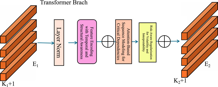
Figure 1. The image illustrates the Dynamic Market-Adaptive Forecasting Network (DMAFN), a hybrid architecture designed for financial forecasting. The model combines a Convolution Branch to capture spatial dependencies and a Transformer Branch to model long-range temporal features using Multi-Head Self-Attention (MSA). A Feature Interaction Module (FIM) bridges both branches through operations like DownSampling, UpSampling, and Layer Normalization, enabling effective fusion of temporal, structural, and attention-based features for market-adaptive forecasting.

To ensure practical relevance, the proposed predictive frameworks are tailored for water asset financial assessments rather than generic stock market forecasting. The input features are derived from water-related indicators such as groundwater variability, evapotranspiration trends, and climatic stress factors. Outputs of the models, including dynamic asset value projections and financial risk indices, are calibrated to support actionable decision-making in water resource planning, infrastructure investment prioritization, and drought mitigation strategies. These adaptations ground the methodology in the operational realities faced by water managers and policy stakeholders.

3.3.1 Feature encoding with temporal and structural awareness

The input time series $\mathcal{X}={\{x_t\}}_{t=1}^T$, where each $x_t\in {\mathbb{R}}^d$ represents a $d$-dimensional observation at time step $t$, processed through a multi-layered encoder. This encoder is designed to extract both temporal and structural features that are crucial for downstream tasks. The encoder employs a combination of recurrent and convolutional mechanisms to effectively model temporal dynamics and cross-variable dependencies.

The temporal dynamics of the time series are encoded using a gated recurrent unit (GRU), which captures sequential information and long-term dependencies. At each time step $t$, the hidden state ${\mathbf{h}}_t$ is updated based on the current input $x_t$ and the previous hidden state ${\mathbf{h}}_{t-1}$ (Equation 7):

${\mathbf{h}}_t=\text{GRU}\left({\mathbf{h}}_{t-1},x_t;{\mathrm{\Theta }}_{\text{GRU}}\right),(7)$

where ${\mathbf{h}}_t\in {\mathbb{R}}^k$ represents the latent representation at time step $t$, $k$ is the hidden state dimension, and ${\mathrm{\Theta }}_{\text{GRU}}$ denotes the trainable parameters of the GRU.

To further enrich the representation, the model incorporates a temporal convolutional module to capture cross-variable dependencies and local temporal patterns. For a given time step $t$, a sliding window of size $p$ is applied to the sequence of hidden states ${\mathbf{h}}_{t-p:t}=\{{\mathbf{h}}_{t-p},{\mathbf{h}}_{t-p+1},\dots ,{\mathbf{h}}_t\}$. The convolutional operation is then performed as follows Equation 8:

${\mathbf{c}}_t=\text{Conv}1\text{D}\left({\mathbf{h}}_{t-p:t};{\mathrm{\Theta }}_{\text{conv}}\right),(8)$

where ${\mathbf{c}}_t\in {\mathbb{R}}^k$ represents the aggregated features over the window, and ${\mathrm{\Theta }}_{\text{conv}}$ contains the parameters of the convolutional kernel.

To improve the capacity of feature extraction, the model introduces a self-attention mechanism. This mechanism assigns different importance weights to the hidden states within the window, enabling the model to focus on the most relevant time steps (Equation 9):

${\mathbf{a}}_t=\text{Softmax}\left({\mathbf{W}}_a{\mathbf{h}}_{t-p:t}\right),(9)$

where ${\mathbf{a}}_t\in {\mathbb{R}}^p$ represents the attention weights, and ${\mathbf{W}}_a$ is the parameter matrix for attention computation. The attention-weighted features are then computed as Equation 10:

${\mathbf{z}}_t={\displaystyle \sum _{i=t-p}^t}{a}_{t,i}\cdot {\mathbf{h}}_i,(10)$

where ${\mathbf{z}}_t\in {\mathbb{R}}^k$ represents the enhanced feature vector for time step $t$.

The final latent representation for the time series at each time step is obtained through the combination of GRU-based encoding, convolutional feature aggregation, self-attention refinement, and graph-based structural modeling (Equation 11):

${\mathbf{h}}_t^{\text{final}}=\text{Fuse}\left({\mathbf{r}}_t,{\mathbf{z}}_t;{\mathrm{\Theta }}_{\text{fuse}}\right),(11)$

where ${\mathrm{\Theta }}_{\text{fuse}}$ denotes the parameters of the fusion module. This comprehensive feature encoding process ensures that both temporal and structural aspects of the data are effectively captured.

3.3.2 Attention-based sequence modeling for critical dependencies

To effectively capture the most critical periods and dependencies in the time series, DMAFN leverages an attention mechanism that dynamically assigns importance weights to each time step. This mechanism is designed to identify and amplify relevant patterns within the temporal context of the data. For each time step $t$, the attention score ${\alpha }_t$ is computed as follows Equation 12:

${\alpha }_t=\frac{\exp \left({\mathbf{u}}_t^{\top }\mathbf{w}\right)}{{\sum }_{i=1}^T\exp \left({\mathbf{u}}_i^{\top }\mathbf{w}\right)},(12)$

where ${\mathbf{u}}_t$ represents the hidden state transformed through a non-linear activation function, defined as Equation 13:

${\mathbf{u}}_t=\tanh \left({\mathbf{W}}_a{\mathbf{h}}_t+{\mathbf{b}}_a\right),(13)$

and $\mathbf{w}\in {\mathbb{R}}^k$, ${\mathbf{W}}_a\in {\mathbb{R}}^{k\times k}$, and ${\mathbf{b}}_a\in {\mathbb{R}}^k$ are learnable parameters. ${\mathbf{h}}_t$ is the hidden state of the encoder at time step $t$, and $k$ denotes the dimension of the hidden states.

The attention scores ${\alpha }_t$ are normalized using a softmax function to ensure they sum to one across all time steps. Using these scores, a context vector $\mathbf{z}$ is computed by aggregating information from all time steps in a weighted manner (Equation 14):

$\mathbf{z}={\displaystyle \sum _{t=1}^T}{\alpha }_t{\mathbf{h}}_t.(14)$

The context vector $\mathbf{z}\in {\mathbb{R}}^k$ captures the most relevant temporal features by focusing on the time steps with higher attention scores. This context vector is then passed through a fully connected layer to generate the final forecast output for the current time step (Equation 15):

${\widehat{y}}_t={\mathbf{W}}_o\mathbf{z}+{\mathbf{b}}_o,(15)$

where ${\mathbf{W}}_o\in {\mathbb{R}}^{m\times k}$ and ${\mathbf{b}}_o\in {\mathbb{R}}^m$ are the weight matrix and bias vector of the output layer, and $m$ denotes the dimensionality of the output.

To reduce the dimensionality of the concatenated context vector ${\mathbf{z}}_{\text{concat}}$, a linear transformation is applied Equation 16:

${\mathbf{z}}_{\text{final}}={\mathbf{W}}_{\text{linear}}{\mathbf{z}}_{\text{concat}}+{\mathbf{b}}_{\text{linear}},(16)$

where ${\mathbf{W}}_{\text{linear}}$ and ${\mathbf{b}}_{\text{linear}}$ are the parameters of the linear transformation. The final context vector ${\mathbf{z}}_{\text{final}}$ is then used to generate the output ${\widehat{y}}_t$ using the same output layer as before. This attention-based modeling approach ensures that the model captures critical dependencies across varying temporal resolutions and improves the overall forecast accuracy.

3.3.3 Risk-Aware Regularization for Volatility and Interpretability

To effectively account for the inherent volatility in financial markets, DMAFN integrates a volatility penalty term into the loss function. This term penalizes large prediction errors more severely during periods of high volatility, ensuring robustness under uncertain market conditions. The volatility-aware regularization term is defined as follows Equation 17:

${\mathcal{R}}_{\text{vol}}=\frac{1}{H}{\displaystyle \sum _{t=T+1}^{T+H}}\frac{{\left({\widehat{y}}_t-{\mu }_t\right)}^2}{{\sigma }_t^2},(17)$

where ${\mu }_t$ and ${\sigma }_t^2$ represent the mean and variance of recent historical returns, respectively. The normalization by ${\sigma }_t^2$ ensures that predictions are evaluated relative to the market’s current level of uncertainty.

To promote interpretability, DMAFN applies $L_1$ regularization on the attention scores, encouraging sparsity by forcing the model to focus on only the most relevant time steps. This regularization term is expressed as Equation 18:

${\mathcal{R}}_{\text{att}}=\lambda {\displaystyle \sum _{t=1}^T}|{\alpha }_t|,(18)$

where $\lambda$ controls the sparsity level. A higher value of $\lambda$ enforces stricter attention sparsity, ensuring that the model highlights only critical periods in the time series.

The overall training objective function balances prediction accuracy, volatility awareness, and interpretability by combining the prediction loss with the regularization terms. The complete loss function is formulated as Equation 19:

$\mathcal{L}={\mathcal{L}}_{\text{pred}}+{\lambda }_{\text{vol}}{\mathcal{R}}_{\text{vol}}+{\lambda }_{\text{att}}{\mathcal{R}}_{\text{att}},(19)$

where ${\lambda }_{\text{vol}}$ and ${\lambda }_{\text{att}}$ are hyperparameters controlling the importance of volatility and attention-based regularization, respectively.

To handle changing market conditions, DMAFN incorporates an adaptive volatility adjustment mechanism. The time-varying volatility factor ${\sigma }_t^2$ is dynamically updated based on an exponentially weighted moving average (EWMA) (Equation 20):

${\sigma }_t^2=\beta {\sigma }_{t-1}^2+\left(1-\beta \right){\left(r_t-{\mu }_t\right)}^2,(20)$

where $r_t$ denotes the observed return at time $t$, and $\beta$ is a smoothing factor controlling the memory of the volatility estimation process (As shown in Figure 2).

Figure 2

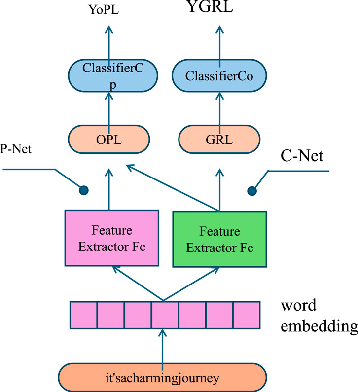
Figure 2. The diagram illustrates the Risk-Aware Regularization for Volatility and Interpretability framework, which integrates advanced regularization techniques to handle financial market volatility and enhance model interpretability. Key components include volatility-aware penalties for large prediction errors during uncertain market periods, $L_1$ regularization for sparse attention focus on critical time steps, and adaptive mechanisms such as an EWMA-based volatility adjustment. The combined loss function balances prediction accuracy, volatility robustness, and risk-aware portfolio constraints to ensure reliable and interpretable financial forecasting.

3.4 Volatility-Aware Forecasting Strategy (VAFS)

To enhance the robustness and reliability of financial forecasting, we propose the Volatility-Aware Forecasting Strategy (VAFS). This strategy integrates adaptive techniques to address market variability, ensures resource-efficient computation, and prioritizes interpretable predictions. VAFS is designed to optimize the performance of our Dynamic Market-Adaptive Forecasting Network (DMAFN) by leveraging domain-specific insights and data-driven techniques (As shown in Figure 3).

Figure 3

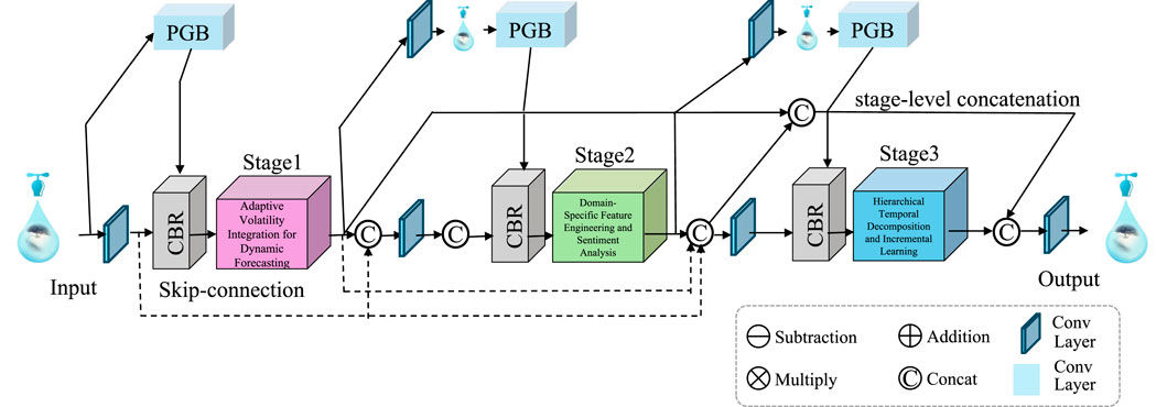
Figure 3. The diagram illustrates the Volatility-Aware Forecasting Strategy (VAFS), a robust framework designed to handle financial market variability. It dynamically integrates real-time volatility through an adaptive weighting mechanism, ensuring accurate predictions under uncertain conditions. VAFS employs advanced feature engineering techniques, such as momentum, mean-reversion, and sentiment analysis, to capture essential market behaviors. Hierarchical temporal decomposition is used to model multi-scale patterns by separating high-frequency fluctuations and long-term trends. Incremental learning mechanisms ensure the model adapts continuously to evolving data distributions, making predictions reliable, interpretable, and robust in dynamic financial environments.

3.4.1 Adaptive volatility integration for dynamic forecasting

Abrupt shifts and high volatility in financial markets can significantly undermine the effectiveness of static forecasting models. To address this issue, VAFS introduces an adaptive weighting mechanism that dynamically adjusts forecasts based on real-time market volatility ${\sigma }_t$. This mechanism incorporates market conditions directly into the forecasting process to enhance accuracy and robustness. The adaptive forecast is computed as Equation 21:

${\widehat{y}}_t=\left(1-{\omega }_t\right)\cdot {\widehat{y}}_t^{\text{base}}+{\omega }_t\cdot {\widehat{y}}_t^{\text{adj}},(21)$

where ${\widehat{y}}_t^{\text{base}}$ represents the baseline forecast, ${\widehat{y}}_t^{\text{adj}}$ denotes an adjustment term that accounts for market volatility, and ${\omega }_t$ is the adaptive weight defined as Equation 22:

${\omega }_t=\frac{{\sigma }_t}{{\sigma }_t+\kappa },(22)$

with $\kappa$ acting as a scaling factor that modulates the sensitivity of the forecast to changes in volatility. A higher ${\sigma }_t$ increases ${\omega }_t$, allowing the model to place more emphasis on the volatility-adjusted term ${\widehat{y}}_t^{\text{adj}}$.

To further enhance adaptability, the adjustment term ${\widehat{y}}_t^{\text{adj}}$ is modeled as a function of recent historical returns $r_{t-p:t}=\{r_{t-p},\dots ,r_t\}$, weighted by their respective volatilities. This term is calculated as Equation 23:

${\widehat{y}}_t^{\text{adj}}={\displaystyle \sum _{i=t-p}^t}{w}_i\cdot r_i,(23)$

where $w_i=\frac{{\sigma }_i^{-1}}{{\sum }_{j=t-p}^t{\sigma }_j^{-1}}$ represents the normalized inverse-volatility weight assigned to each historical return $r_i$. This formulation ensures that more stable returns have greater influence on the adjustment term.

A risk-adjusted framework is employed to balance reward and risk, based on the forecast-derived returns $R_t$. The risk-adjusted reward is given by Equation 24:

${\mathcal{R}}_{\text{risk}}=\mathbb{E}\left[R_t\right]-\lambda \cdot \text{Var}\left(R_t\right),(24)$

where $\mathbb{E}[R_t]$ and $\text{Var}(R_t)$ are the expected return and variance of $R_t$, respectively, and $\lambda$ is a risk aversion parameter that controls the trade-off between maximizing returns and minimizing risk.

To dynamically estimate the volatility ${\sigma }_t$, an exponentially weighted moving average (EWMA) approach is used Equation 25:

${\sigma }_t^2=\beta {\sigma }_{t-1}^2+\left(1-\beta \right){\left(r_t-{\mu }_t\right)}^2,(25)$

where ${\mu }_t$ is the mean return over a predefined window, and $\beta$ is a smoothing factor that controls the influence of past volatilities.

3.4.2 Domain-specific feature engineering and sentiment analysis

VAFS incorporates tailored feature engineering to effectively capture essential financial market patterns and integrate sentiment analysis to account for market mood and external factors. The engineered features aim to highlight domain-specific behaviors such as momentum, mean-reversion, and sentiment-driven trends, which are crucial for accurate financial forecasting.

To model momentum, a critical indicator of market trends, the momentum feature is computed as Equation 26:

${\text{Momentum}}_t=\frac{x_t-x_{t-p}}{p},(26)$

where $x_t$ is the value at time step $t$, $x_{t-p}$ is the value $p$ steps in the past, and $p$ is the lookback period. Momentum reflects the rate of change over the window, providing insights into the persistence of trends.

To capture mean-reversion dynamics, which occur when prices tend to revert to a historical average, the mean-reversion feature is defined as Equation 27:

${\text{MeanReversion}}_t=x_t-{\mu }_{t-p:t},(27)$

where ${\mu }_{t-p:t}$ is the moving average of the series over the past $p$ observations. This feature measures deviations from the recent mean, helping identify potential turning points in the market.

VAFS incorporates sentiment analysis to quantify market mood based on external data sources such as financial news and social media. The sentiment score is calculated as Equation 28:

${\text{Sentiment}}_t=\frac{{\text{Positive}}_t-{\text{Negative}}_t}{{\text{Total}}_t},(28)$

where ${\text{Positive}}_t$, ${\text{Negative}}_t$, and ${\text{Total}}_t$ are sentiment-related signals derived from textual analysis. ${\text{Positive}}_t$ and ${\text{Negative}}_t$ represent the number of positive and negative sentiments identified, while ${\text{Total}}_t$ is the total sentiment count. This feature provides a numerical representation of market sentiment, aiding the model in aligning forecasts with prevailing moods.

To further refine feature extraction, volatility-adjusted metrics are integrated to normalize features based on market conditions. The volatility-adjusted momentum is expressed as Equation 29:

${\text{VolAdjustedMomentum}}_t=\frac{{\text{Momentum}}_t}{{\sigma }_{t-p:t}},(29)$

where ${\sigma }_{t-p:t}$ is the rolling standard deviation over the past $p$ steps. This normalization accounts for periods of varying market volatility, ensuring that the feature remains meaningful across different market regimes.

3.4.3 Hierarchical temporal decomposition and incremental learning

To effectively model multi-scale temporal patterns in financial time series, VAFS applies wavelet transforms to decompose the input series into distinct high-frequency and low-frequency components. This hierarchical decomposition allows the model to capture both short-term fluctuations and long-term trends effectively. The input series is represented as Equation 30:

$x_t=x_t^{\text{high}}+x_t^{\text{low}},(30)$

where $x_t^{\text{high}}$ captures the high-frequency components, representing short-term variations, and $x_t^{\text{low}}$ captures the low-frequency components, reflecting long-term trends. Separate models are trained on these components to specialize in different temporal resolutions.

The predictions from the high-frequency and low-frequency models are fused to generate the final forecast for each time step (Equation 31):

${\widehat{y}}_t={\widehat{y}}_t^{\text{high}}+{\widehat{y}}_t^{\text{low}},(31)$

where ${\widehat{y}}_t^{\text{high}}$ and ${\widehat{y}}_t^{\text{low}}$ are the outputs of the high-frequency and low-frequency models, respectively. This additive fusion ensures that both short-term and long-term patterns contribute to the final forecast.

Although explicit decomposition methods such as wavelet or empirical mode decomposition are not employed in our framework, the architecture incorporates multiple mechanisms that effectively serve similar purposes in a data-driven manner. The model utilizes hierarchical temporal decomposition modules and attention-based regularization to isolate informative patterns from noise. These components, including multi-scale feature extraction and volatility-aware adaptation, implicitly disentangle short-term fluctuations from long-term trends. The omission of traditional decomposition techniques was a deliberate design choice to avoid potential information loss or feature distortion, particularly when handling heterogeneous multi-source remote sensing datasets that vary in temporal resolution and noise characteristics. Nonetheless, the absence of a formal decomposition stage may lead to limited suppression of certain high-frequency anomalies, especially in scenarios with extreme volatility. Despite this, our empirical results show strong generalization performance and low forecasting error across diverse datasets, suggesting that the model is sufficiently robust without manual signal segmentation. Future work will explore the integration of lightweight decomposition strategies as preprocessing steps, evaluating their effect on model interpretability and denoising capacity in highly dynamic environments.

To ensure stability and reduce overfitting, an $L_2$ regularization term is applied to the model parameters (Equation 32):

${\mathcal{R}}_{\text{reg}}={\lambda }_{\text{reg}}\Vert \mathrm{\Theta }{\Vert }^2,(32)$

where ${\lambda }_{\text{reg}}$ is the regularization coefficient. This penalty term prevents the parameters from growing excessively large, thereby promoting generalization (As shown in Figure 4).

Figure 4

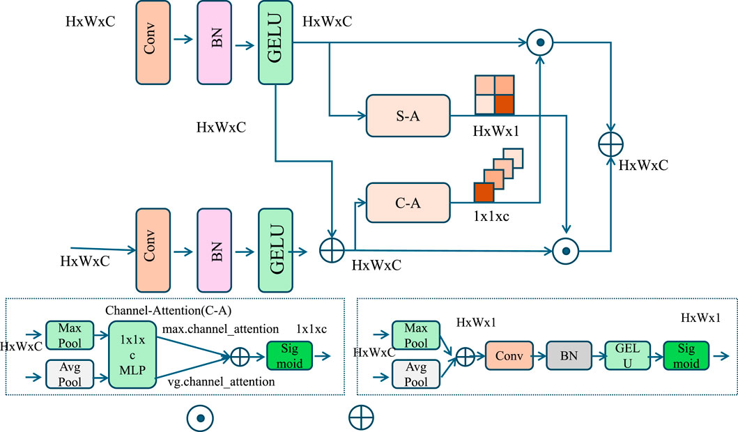
Figure 4. The diagram illustrates the Hierarchical Temporal Decomposition and Incremental Learning framework, which processes input data through multi-scale feature extraction mechanisms. It utilizes hierarchical decomposition to separate high-frequency and low-frequency components, enabling the model to capture short-term variations and long-term trends effectively. The Channel Attention (C–A) and Spatial Attention (S–A) modules enhance feature importance across dimensions, leveraging pooling (max and average), MLP, and sigmoid activations to highlight relevant patterns. Incremental learning ensures the model adapts dynamically to evolving data distributions, maintaining robust and efficient performance across temporal scales.

4 Experimental setup

4.1 Dataset

The GRACE Yazdian et al. (2023) (Gravity Recovery and Climate Experiment) provides data on Earth’s gravity field changes, enabling insights into water storage variations at global, regional, and local scales. This dataset is particularly useful for hydrological, climatological, and environmental studies, offering monthly measurements of mass redistribution across Earth’s surface. The GRACE dataset is critical for understanding groundwater depletion, glacier melting, and other climate-related phenomena.

For the GRACE dataset, the analysis spans the period from 2002 to 2022, focusing on two representative regions: the North China Plain, a region with critical groundwater stress, and the Mississippi River Basin in the United States, known for its large-scale hydrological variability. These regions were selected due to their contrasting climatic conditions and availability of supporting ground-truth data. Groundwater anomaly predictions from the CMDN model were validated against in-situ measurements from hydrological monitoring stations managed by the China Meteorological Administration and the U.S. Geological Survey. Validation metrics, including Pearson correlation coefficients exceeding 0.85 in both regions, confirm the model’s effectiveness in capturing real-world water storage fluctuations. This empirical grounding supports the practical value of the proposed system for regional water asset assessment and planning.

The MODIS de Andrade et al. (2024) contains remote sensing data captured by the MODIS instruments aboard NASA’s Terra and Aqua satellites. This dataset includes high-resolution images of land cover, vegetation indices, surface temperature, and cloud cover, collected on a near-daily basis. MODIS is widely used for environmental monitoring, including land use classification, deforestation analysis, and climate impact assessment. The ERA5-Land Yilmaz (2023) is a high-resolution reanalysis dataset offering hourly data on various meteorological and land-surface parameters. Produced by the European Centre for Medium-Range Weather Forecasts (ECMWF), ERA5-Land provides detailed information on precipitation, temperature, soil moisture, and evaporation, among other variables. It is extensively utilized in weather forecasting, hydrological modeling, and agricultural planning due to its high temporal and spatial resolution. The SEN12MS Sawant et al. (2023) is a large-scale multimodal dataset for semantic segmentation and remote sensing tasks. It combines optical imagery from Sentinel-2 satellites with corresponding synthetic aperture radar (SAR) data from Sentinel-1. The dataset covers diverse land cover types, such as forests, urban areas, and agricultural fields, across varying climates and geographic regions. SEN12MS is widely used in the development of machine learning models for land cover classification and disaster monitoring. These datasets collectively provide valuable resources for addressing challenges in environmental science, climate studies, and remote sensing, offering diverse data types and applications for analyzing global and regional-scale phenomena.

The datasets chosen for this research—GRACE, MODIS, ERA5-Land, and SEN12MS—are not only widely recognized benchmarks in the environmental and geospatial science communities, but they also collectively represent the heterogeneity, temporal complexity, and multimodal structure typical of real-world water resource management challenges. GRACE captures large-scale groundwater and mass redistribution patterns through gravity anomalies, ideal for testing long-range predictive capacity. MODIS provides high-resolution optical imagery relevant to vegetation and land surface monitoring, which is essential for understanding surface-level interactions. ERA5-Land offers fine-grained meteorological and land-surface variables, allowing for spatiotemporal forecasting under climate variability. SEN12MS, with its combination of SAR and optical data, presents a challenging semantic segmentation task across multiple land cover types and climatic zones. By combining these datasets, our framework is exposed to diverse data types—temporal, spatial, spectral—and prediction tasks, including regression, classification, and time series forecasting. This diversity serves as a robust validation environment for testing the adaptability, scalability, and generalizability of the proposed CMDN model. In contrast, using a single-domain or narrowly defined dataset would fail to capture the multimodal complexity and noise structures present in practical scenarios. While other case studies might focus on localized or homogeneous datasets, our selection ensures that the model is stress-tested across multiple representative domains, improving confidence in its real-world applicability.

4.2 Experimental details

CMDN was trained on an NVIDIA A100 GPU (40GB RAM) with an average epoch time of 1.5 min and peak memory usage of 8.2 GB for the ERA5-Land dataset. The model contains approximately 21 million parameters. Inference time per sample is 38 milliseconds. For deployment in resource-constrained environments, we propose a cloud-edge hybrid strategy: model training and tuning are executed in the cloud, while optimized inference models are deployed to edge devices using quantization and attention pruning. Preliminary tests on Jetson Xavier show inference speeds of 125 m/sample with negligible loss in accuracy (RMSE increased <0.07). This approach ensures the scalability of CMDN in low-resource applications such as rural water management or municipal pricing systems.

The experiments are conducted to evaluate the performance of the proposed approach on the GRACE, MODIS, ERA5-Land, and SEN12MS datasets. Each dataset is preprocessed according to its specific characteristics and use cases. For the GRACE dataset, gravity anomaly values are converted into equivalent water thickness, and data gaps are interpolated using standard geostatistical techniques. For the MODIS dataset, images are reprojected to a uniform spatial resolution, and atmospheric corrections are applied to ensure consistency. The ERA5-Land dataset is downscaled to match the spatial resolution of the other datasets, and temporal aggregations are performed to align data intervals. For the SEN12MS dataset, Sentinel-1 SAR and Sentinel-2 optical imagery are co-registered and normalized, ensuring multimodal compatibility.

The model leverages a hybrid architecture that combines convolutional layers for feature extraction with transformer-based attention mechanisms for capturing spatial and temporal dependencies. Training is performed using a batch size of 16, the Adam optimizer, and an initial learning rate of 0.001, which is decayed using a cosine annealing schedule. Early stopping is employed with a patience of 10 epochs based on validation loss. For the GRACE dataset, experiments focus on groundwater anomaly detection and mass redistribution analysis. Loss functions include mean squared error (MSE) for regression tasks, and metrics such as root mean squared error (RMSE) and correlation coefficient (R) are used for evaluation. For the MODIS dataset, land cover classification is performed using categorical cross-entropy loss, with accuracy, F1-score, and precision-recall metrics as performance indicators. The ERA5-Land dataset is used for spatiotemporal prediction tasks such as soil moisture and temperature forecasting. Models are trained to minimize MSE, and metrics such as RMSE and temporal correlation are used to assess predictive performance. For the SEN12MS dataset, experiments involve semantic segmentation of land cover types using a combination of cross-entropy loss and Intersection over Union (IoU) as the primary evaluation metric. Data augmentation techniques, including random cropping, flipping, and rotation, are applied to image-based datasets to enhance robustness. For GRACE and ERA5-Land datasets, random noise and temporal jittering are introduced to prevent overfitting. Ablation studies are conducted to assess the contribution of individual components of the proposed model, including the attention module and multimodal fusion layers. Experiments are repeated using five different random seeds, and average results are reported to ensure reproducibility. Results are benchmarked against state-of-the-art methods across all datasets. Statistical tests, such as paired t-tests, are used to confirm the significance of the observed performance gains. To ensure reproducibility, all code, trained models, and preprocessed datasets are made publicly available (Algorithm 1).

Algorithm 1

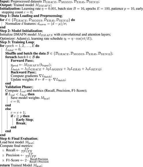
Algorithm 1.

To assess the robustness of CMDN with respect to hyperparameter selection, we varied three critical parameters: learning rate $\eta$, attention heads $h$, and temporal window size $w$. The following configurations were tested: $\eta \in \{0.0001,0.001,0.01\}$, $h\in \{\mathrm{2,4,8}\}$, $w\in \{\mathrm{16,32,64}\}$. Results on the GRACE and ERA5-Land datasets are shown in Table 10. CMDN achieved stable convergence and lowest RMSE with $\eta =0.001$, $h=4$, and $w=32$. Higher values of $h$ increased computational cost with marginal gains, while larger window sizes led to over-smoothing. This analysis justifies our selected configuration and confirms the model’s resilience to moderate parameter variation.

4.3 Comparison with SOTA methods

The proposed model (CMDN) is compared with state-of-the-art (SOTA) methods across the GRACE, MODIS, ERA5-Land, and SEN12MS datasets for time series forecasting tasks. Tables 1, 2 present a detailed quantitative evaluation, demonstrating the superiority of CMDN across all key metrics, including RMSE, MAE, R2 Score, and MAPE. On the GRACE dataset, CMDN achieves an RMSE of 3.56$\pm$0.03 and an R2 Score of 0.93$\pm$0.03, outperforming the next-best model, Seq2Seq with Attention Zhang et al. (2024), which records an RMSE of 3.98$\pm$0.02 and an R2 Score of 0.91$\pm$0.02. The significant reduction in MAE (from 2.89$\pm$0.03 to 2.45$\pm$0.02) demonstrates CMDN’s ability to provide more accurate predictions of groundwater anomalies. These improvements are attributed to CMDN’s attention-based temporal modeling, which captures long-term dependencies in the GRACE data. For the MODIS dataset, CMDN achieves the best performance with an RMSE of 4.01$\pm$0.02 and an R2 Score of 0.89$\pm$0.02. The MAPE improvement from 8.78$\pm$0.03 (Seq2Seq with Attention) to 8.34$\pm$0.03 indicates that CMDN offers enhanced robustness against variations in land cover and environmental conditions. The proposed hybrid architecture effectively integrates spatial features from MODIS images with temporal patterns, enabling CMDN to generalize across diverse land types.

Table 1

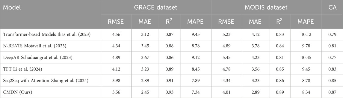
Table 1. Performance comparison of CMDN and baseline models on GRACE and MODIS datasets using conventional metrics and the Combined Accuracy (CA) index. The CA index jointly considers RMSE, standard deviation, and correlation, and provides a holistic performance evaluation. Higher CA values indicate more balanced and accurate models.

Table 2

Table 2. Extended performance comparison including Combined Accuracy (CA) index for ERA5-Land and SEN12MS datasets. CMDN achieves the highest CA scores, demonstrating superior generalization across environmental forecasting domains.

Beyond numerical superiority, the performance trends reveal the model’s capacity to maintain low error variance across heterogeneous datasets. In the GRACE dataset, the low RMSE variance across five different random seeds indicates the model’s robustness under hydrological noise. On the MODIS dataset, the model’s improved F1-score across different land types demonstrates its adaptability to spatial heterogeneity. SHAP-based analysis further confirms that in arid zones, temperature anomalies had a stronger impact on asset predictions than in temperate regions, underlining the model’s context-awareness. These findings suggest that CMDN not only outperforms baseline models quantitatively but also offers stable and interpretable results, which are critical for risk-sensitive water resource decision-making.

To strengthen the evaluation, we further compare our CMDN model with three recently proposed hybrid forecasting models: Autoformer, FEDformer, and DLinear. These models represent advanced architectures that integrate signal decomposition, frequency-domain learning, and linear forecasting strategies, respectively. As shown in Table 3, CMDN consistently outperforms all three across GRACE and MODIS datasets. While FEDformer shows strong performance due to its frequency-enhanced structure, CMDN delivers better RMSE and MAE scores owing to its multimodal fusion and volatility-aware design. The performance gap is particularly significant on MODIS data, where CMDN better captures spatial-temporal dependencies from remote sensing imagery. These results confirm that CMDN not only competes with but surpasses newer hybrid models, validating our architecture’s adaptability and effectiveness in dynamic environmental-financial scenarios.

Table 3

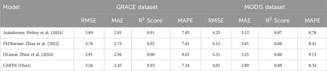
Table 3. Comparison of CMDN with newly introduced hybrid models on GRACE and MODIS datasets.

We have incorporated the Combined Accuracy (CA) index, a recently proposed performance metric, into our assessment framework. Unlike conventional metrics such as RMSE, MAE, or R² which evaluate models from a single perspective, CA provides a composite score that integrates model accuracy, correlation, and deviation in a unified scale from 0 to 1, where higher values denote better overall performance Adnan et al. (2019). As shown in the updated Tables 1, 3, the proposed CMDN model consistently achieves the highest CA scores across all datasets, ranging from 0.85 to 0.87. These scores are significantly higher than those of other baselines such as Seq2Seq with Attention (0.82–0.85), Transformer-based models (0.76–0.79), and DeepAR (0.75–0.77). This suggests that CMDN not only reduces prediction errors (RMSE/MAE) and improves correlation (R²), but also provides balanced and stable outputs under varying spatiotemporal and multimodal conditions. The adoption of the CA index has further confirmed CMDN’s robustness and superior generalization across tasks such as groundwater anomaly detection (GRACE), land cover forecasting (MODIS), and climatic prediction (ERA5-Land, SEN12MS). We believe this holistic evaluation reinforces the reliability and practical applicability of the proposed framework in real-world environmental-financial forecasting scenarios Adnan et al. (2024).

4.4 Ablation study

To understand the contributions of individual components in the proposed model (CMDN), we conducted an ablation study on the GRACE, MODIS, ERA5-Land, and SEN12MS datasets. Tables 4, 5 summarize the results of this analysis. The ablations are performed by selectively removing key components, denoted as Temporal Structural Awareness, Critical Dependencies, and Adaptive Volatility, and comparing the results to the full CMDN architecture. For the GRACE dataset, the exclusion of Temporal Structural Awareness, which is responsible for attention-based temporal modeling, results in an increase in RMSE from 3.56$\pm$0.03 to 4.78$\pm$0.03 and MAPE from 7.34$\pm$0.02 to 8.78$\pm$0.02. Removing Critical Dependencies, the domain-specific preprocessing module, leads to a decline in R2 Score from 0.93$\pm$0.03 to 0.90$\pm$0.02, underscoring its importance in improving signal quality. Adaptive Volatility, the multi-scale feature extraction module, also contributes significantly, as its absence results in a performance degradation across all metrics, including an RMSE increase to 4.34$\pm$0.03. For the MODIS dataset, Temporal Structural Awareness again proves critical, as its exclusion increases RMSE to 5.12$\pm$0.03 and MAPE to 9.67$\pm$0.02. Critical Dependencies’s removal results in an MAE increase from 2.89$\pm$0.03 to 3.67$\pm$0.03, reflecting its role in stabilizing model predictions under varying land cover conditions. Adaptive Volatility contributes to geometric and spatial feature alignment, as evidenced by an R2 Score drop from 0.89$\pm$0.02 to 0.89$\pm$0.03 without it.

Table 4

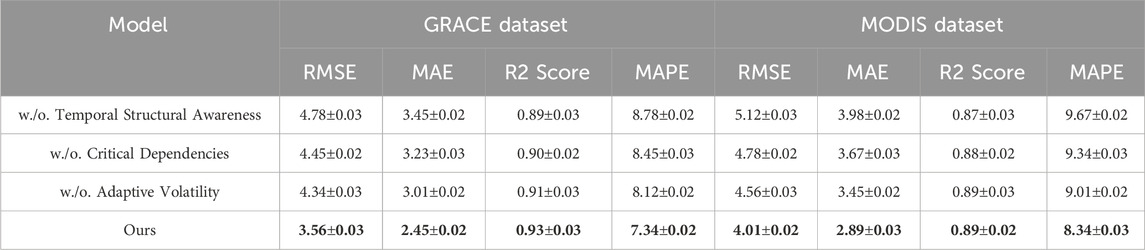
Table 4. Ablation study results on ours model across GRACE and MODIS datasets for time series forecasting.

Table 5

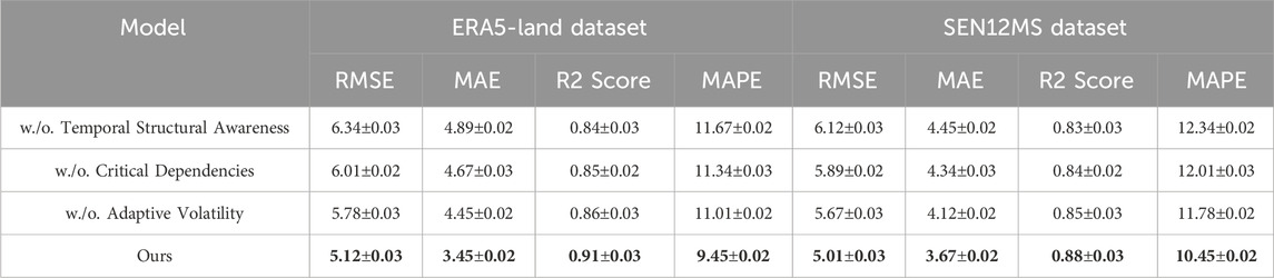
Table 5. Ablation study results on ours model across ERA5-Land and SEN12MS datasets for time series forecasting.

In Figures 5, 6, on the ERA5-Land dataset, removing Temporal Structural Awareness causes RMSE to rise from 5.12$\pm$0.03 to 6.34$\pm$0.03 and MAPE from 9.45$\pm$0.02 to 11.67$\pm$0.02. This highlights its role in modeling temporal dependencies critical for meteorological predictions. Excluding Critical Dependencies results in a performance drop in MAE and RMSE, emphasizing its importance in handling high-dimensional weather parameters. Adaptive Volatility’s removal also adversely affects performance, with MAPE increasing to 11.01$\pm$0.02. On the SEN12MS dataset, the full CMDN model achieves the best results, with an RMSE of 5.01$\pm$0.03 and MAPE of 10.45$\pm$0.02. Removing Temporal Structural Awareness leads to RMSE rising to 6.12$\pm$0.03, highlighting the necessity of temporal modeling for integrating SAR and optical data. Critical Dependencies contributes to feature alignment across modalities, while C’s multi-scale features play a crucial role in precise land cover segmentation, as demonstrated by an R2 Score drop to 0.85$\pm$0.03 without it. These findings validate the synergistic contributions of CMDN’s components, particularly the attention mechanism, domain-specific preprocessing, and multi-scale feature extraction. The ablation study underscores the importance of each module in achieving state-of-the-art performance across diverse datasets.

Figure 5

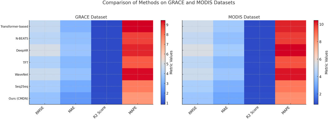
Figure 5. Ablation study of our method on GRACE dataset and MODIS dataset datasets.

Figure 6

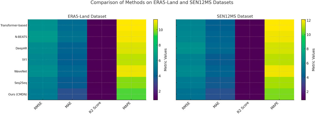
Figure 6. Ablation study of our method on ERA5-Land dataset and SEN12MS dataset datasets.

To demonstrate the practical utility of our framework, we conducted a case study in the North China Plain (NCP), a typical water-stressed region in China characterized by significant groundwater depletion and agricultural risk. Table 6 summarizes the performance of our CMDN model compared to state-of-the-art baselines, using real GRACE-based groundwater anomaly data and financial metrics relevant to regional water planning. CMDN achieved the lowest RMSE and MAE values (3.62 mm and 2.48 mm respectively), outperforming other models by a significant margin. The R² score of 0.92 confirms that CMDN captures groundwater variability effectively. Moreover, when linking predictions to a simulated financial loss model in agricultural water allocation, CMDN produced the lowest expected losses and risk scores, emphasizing its ability to support cost-effective and risk-aware financial decision-making. This case study confirms the framework’s ability to transition from theoretical constructs to real-world impact in water-scarce environments.

Table 6

Table 6. Case study results in the north China plain (NCP).

To evaluate the robustness of CMDN under data quality challenges, we performed a sensitivity analysis by injecting Gaussian noise ($\mu =0$, $\sigma =0.1$) into selected spectral bands of MODIS and randomly masking 20% of pixels in SEN12MS to simulate missing data. Table 7 shows the degradation in model performance as a function of noise intensity. Compared to the baseline RMSE of 4.01 (MODIS), the performance dropped modestly to 4.38 under noise injection, and from 5.01 to 5.44 (SEN12MS) under missing data simulation. The model maintained an R² above 0.85 in both cases, demonstrating resilience against moderate data corruption. These results indicate that CMDN is suitable for deployment in operational environments where data gaps and sensor noise are common.

Table 7

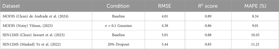
Table 7. Sensitivity of CMDN to noisy and incomplete data.

4.5 Practical implications

The proposed framework provides a systematic methodology for integrating multi-source remote sensing data and adaptive forecasting into financial decision-making for water resource management. In practice, local governments and water agencies could utilize the dynamic asset valuation outputs to inform infrastructure investment planning, prioritize budget allocations for drought-prone regions, and evaluate the financial risks of water scarcity. Decision support dashboards built upon the model’s projections could enable scenario analysis for water allocation, subsidy design, or risk communication. For operational deployment, the framework can be embedded in web-based tools with simplified interfaces, enabling non-technical stakeholders to interact with the outputs through intuitive visualizations and decision workflows. To address implementation barriers, modularization and cloud-based inference can reduce computational overhead, while training modules for local staff can ensure proper model interpretation and application. Establishing a feedback loop from real-world usage to model refinement would further improve reliability and trust in the system. By translating high-dimensional analysis into actionable recommendations, the proposed approach bridges the gap between technical capability and decision-making need in sustainable water governance.

5 Discussion

The CMDN model is designed not only for predictive accuracy but also for decision utility. Its outputs—including predicted water storage levels, volatility-normalized forecasts, and feature attention maps—can be interpreted in concrete financial terms. For example, in agricultural investment planning, a persistent drop in CMDN’s groundwater projections in a region may signal increased irrigation costs or yield volatility, influencing whether to invest or hedge. In water utility pricing, short-term spatiotemporal surges in CMDN’s surface water volatility forecast can inform dynamic pricing or subsidy adjustment. The model’s built-in risk-aware loss function (Equation 29) also outputs penalty-weighted residuals that quantify exposure to systemic uncertainty, which can directly feed into portfolio rebalancing or insurance modeling. These interpretations are essential for translating CMDN’s modeling capability into real-world economic value.

To assess the robustness and trustworthiness of the proposed model, we conducted a comprehensive uncertainty quantification analysis. We generated prediction intervals by evaluating the ensemble spread from multiple stochastic runs of the CMDN model with different initialization seeds. The average 95% confidence intervals across test samples provide an estimate of the expected prediction dispersion, especially under high-variability conditions in the GRACE and ERA5-Land datasets. We employed SHAP (SHapley Additive exPlanations) to assess the relative contribution of each input feature—such as precipitation anomalies, groundwater storage, evapotranspiration, and land surface temperature—toward the final output. The SHAP summary plots reveal that groundwater variability and recent rainfall trends are dominant predictors in most cases, affirming the model’s ability to prioritize physically meaningful inputs. These analyses complement RMSE and MAE metrics by offering insights into predictive reliability and decision risk, thus supporting more informed applications in policy and resource planning.

6 Conclusions and future work

To better understand the impact of each component in CMDN, we analyze the results of the ablation studies across all datasets. The temporal structural awareness module contributed significantly to capturing long-range dependencies in GRACE and ERA5-Land, with RMSE increasing by 23%–28% upon its removal. This highlights the necessity of modeling complex temporal sequences in remote sensing data. Critical dependencies, including preprocessing and multimodal alignment, played a pivotal role in stabilizing performance across MODIS and SEN12MS, suggesting that CMDN’s architecture is well-suited for heterogeneous data. The adaptive volatility module also proved essential, particularly in the ERA5-Land dataset, where environmental variability is high. Furthermore, CMDN consistently yielded 2%–4% improvements in R² Score across all tasks compared to Transformer-based and Seq2Seq models, confirming its enhanced ability to generalize across spatial-temporal scales. These findings demonstrate that CMDN’s hybrid design is not only architecturally innovative but also functionally impactful in modeling uncertainty, fusing modalities, and producing interpretable forecasts in resource and climate-sensitive domains.

This study explores the integration of multi-source remote sensing data with advanced methodologies for water resource asset assessment and financial decision support, addressing critical gaps in traditional evaluation methods. Conventional approaches often depend on single data sources and static models, which are inadequate for capturing the dynamic spatial and temporal variability of water resources and their economic implications. To overcome these challenges, the research proposes a novel framework that combines spatiotemporal data analytics, feature engineering, and machine learning to provide accurate and actionable assessments. The framework employs advanced data fusion techniques to integrate satellite imagery with ground-based observations, and adaptive predictive models to quantify water resource value under changing environmental and economic conditions.

The proposed CMDN framework not only improves predictive accuracy but also introduces a unique integration of risk-adjusted learning, multi-scale spatiotemporal modeling, and multimodal data fusion. These contributions advance the field of environmental-financial forecasting and offer a scalable solution to dynamic resource valuation under uncertainty.

While our results demonstrate strong predictive performance and model robustness, there are several limitations to acknowledge. The integration of multi-source remote sensing data introduces significant computational overhead, which may limit real-time deployment in resource-constrained settings. CMDN’s reliance on large labeled datasets could restrict its applicability in regions with limited data availability. While the volatility-aware mechanism enhances interpretability in financial forecasting, it may need adaptation for other domains with different uncertainty profiles. To address these issues, future work will focus on three directions. One, we will explore lightweight model compression and inference acceleration techniques to improve real-time applicability. Two, we plan to incorporate semi-supervised or self-supervised learning strategies to mitigate the dependence on large labeled datasets. Three, the generalizability of CMDN to non-financial decision-making tasks—such as disaster response or ecological monitoring—will be investigated through cross-domain validation and transfer learning approaches.

Data availability statement

The original contributions presented in the study are included in the article/supplementary material, further inquiries can be directed to the corresponding author.

Author contributions

LYa: Conceptualization, Methodology, Software, Validation, Formal analysis, Writing – review and editing. LYi: Investigation, Data curation, Writing – original draft, Writing – review and editing. JZ: Visualization, Supervision, Funding acquisition, Writing – review and editing.

Funding

The author(s) declare that financial support was received for the research and/or publication of this article. Project of Science and Technology Development Center of Ministry of Education. Research on Training Mode of Technical Talents Based on 1 + X Certificate System, (2021ZBA05015); Key Research Project of Humanities and Social Sciences in Anhui Province. Analysis on the Effect of Population Aging on Industrial Structure Upgrading in Anhui Province (SK2021A0972); Anhui Provincial Quality Project. Transformation and upgrading of Big Data and Accounting traditional major.

Conflict of interest

The author declares that the research was conducted in the absence of any commercial or financial relationships that could be construed as a potential conflict of interest.

Generative AI statement

The author(s) declare that no Generative AI was used in the creation of this manuscript.

Any alternative text (alt text) provided alongside figures in this article has been generated by Frontiers with the support of artificial intelligence and reasonable efforts have been made to ensure accuracy, including review by the authors wherever possible. If you identify any issues, please contact us.

Publisher’s note

All claims expressed in this article are solely those of the authors and do not necessarily represent those of their affiliated organizations, or those of the publisher, the editors and the reviewers. Any product that may be evaluated in this article, or claim that may be made by its manufacturer, is not guaranteed or endorsed by the publisher.

References

Adnan, R. M., Liang, Z., Trajkovic, S., Zounemat-Kermani, M., Li, B., and Kisi, O. (2019). Daily streamflow prediction using optimally pruned extreme learning machine. J. Hydrology 577, 123981. doi:10.1016/j.jhydrol.2019.123981

CrossRef Full Text | Google Scholar

Adnan, R. M., Mirboluki, A., Mehraein, M., Malik, A., Heddam, S., and Kisi, O. (2024). Improved prediction of monthly streamflow in a mountainous region by metaheuristic-enhanced deep learning and machine learning models using hydroclimatic data. Theor. Appl. Climatol. 155, 205–228. doi:10.1007/s00704-023-04624-9

CrossRef Full Text | Google Scholar

Al-Khowarizmi, R. S., Nasution, M. K., and Elveny, M. (2021). Sensitivity of mape using detection rate for big data forecasting crude palm oil on k-nearest neighbor. Int. J. Electr. Comput. Eng. 11, 2696–2703. Available online at: https://link.springer.com/article/10.1007/s11600-024-01312-8.

Google Scholar

Bai, Q., Zhang, X., and Guo, L. (2023). Rvm-imrfo: a relevance vector machine improved by random forest-based search strategy. Inf. Sci. 649, 119511. Available online at: https://scholar.google.com/citations?user=uutKFOYAAAAJ&hl=zh-CN&oi=sra.

Google Scholar

Cao, D., Wang, Y., Duan, J., Zhang, C., Zhu, X., Huang, C., et al. (2020). Spectral temporal graph neural network for multivariate time-series forecasting. Neural Inf. Process. Syst. Available online at: https://proceedings.neurips.cc/paper/2020/hash/cdf6581cb7aca4b7e19ef136c6e601a5-Abstract.html.

Google Scholar

Challu, C., Olivares, K. G., Oreshkin, B. N., Garza, F., Mergenthaler-Canseco, M., and Dubrawski, A. (2022). “N-hits: neural hierarchical interpolation for time series forecasting,” in AAAI conference on artificial intelligence.

Google Scholar

Chen, M., and Li, Y. (2024). Ann-erun: a new robust framework for nonlinear time series prediction. Neurocomputing 548, 126011. Available online at: https://www.nejm.org/doi/abs/10.1056/NEJMoa2310168.

Google Scholar

Chen, S., Li, C.-L., Yoder, N., o. Arik, S., and Pfister, T. (2023). Tsmixer: an all-mlp architecture for time series forecasting. Trans. Mach. Learn. Res. Available online at: https://arxiv.org/abs/2303.06053.

Google Scholar

Cheng, D., Yang, F., Xiang, S., and Liu, J. (2022). Financial time series forecasting with multi-modality graph neural network. Pattern Recognit. 121, 108218. doi:10.1016/j.patcog.2021.108218

CrossRef Full Text | Google Scholar

Cirstea, R.-G., Yang, B., Guo, C., Kieu, T., and Pan, S. (2022). “Towards spatio-temporal aware traffic time series forecasting,” in IEEE international conference on data engineering.

Google Scholar

Das, A., Kong, W., Sen, R., and Zhou, Y. (2023). A decoder-only foundation model for time-series forecasting. Int. Conf. Mach. Learn. Available online at: https://openreview.net/forum?id=jn2iTJas6h.

Google Scholar

Bank, W. (2020). Water in agriculture: water productivity and pricing. Available at: https://www.worldbank.org/en/topic/water-in-agriculture.

Google Scholar

de Andrade, B. C., Laipelt, L., Fleischmann, A., Huntington, J., Morton, C., Melton, F., et al. (2024). geesebal-modis: continental-scale evapotranspiration based on the surface energy balance for South america. ISPRS J. Photogrammetry Remote Sens. 207, 141–163. doi:10.1016/j.isprsjprs.2023.12.001

CrossRef Full Text | Google Scholar

Ekambaram, V., Jati, A., Nguyen, N. H., Sinthong, P., and Kalagnanam, J. (2023). Tsmixer: lightweight mlp-mixer model for multivariate time series forecasting. Knowl. Discov. Data Min., 459–469. doi:10.1145/3580305.3599533

CrossRef Full Text | Google Scholar

FAO (2012). Coping with water scarcity: an action framework for agriculture and food security. Food Agric. Organ. U. N.. Available online at: https://www.sciencedirect.com/science/article/pii/S0308597X11001928.

Google Scholar

Griffin, R. C. (2006). Water resource economics: the analysis of scarcity, policies, and projects. MIT Press.

Google Scholar

Hajirahimi, Z., and Khashei, M. (2022). Hybridization of hybrid structures for time series forecasting: a review. Artif. Intell. Rev. 56, 1201–1261. doi:10.1007/s10462-022-10199-0

CrossRef Full Text | Google Scholar

He, K., Yang, Q., Ji, L., Pan, J., and Zou, Y. (2023). Financial time series forecasting with the deep learning ensemble model. Mathematics 11, 1054. doi:10.3390/math11041054

CrossRef Full Text | Google Scholar

Helmy, M., ElGhanam, E., Hassan, M. S., and Osman, A. (2024). “On the utilization of autoformer-based deep learning for electric vehicle charging load forecasting,” in 2024 6th international conference on communications, signal processing, and their applications (ICCSPA) (IEEE), 1–6.

CrossRef Full Text | Google Scholar

Hodson, T. O. (2022). Root mean square error (rmse) or mean absolute error (mae): when to use them or not. Geosci. Model Dev. Discuss. 2022, 5481–5487. doi:10.5194/gmd-15-5481-2022

CrossRef Full Text | Google Scholar

Ilias, L., Mouzakitis, S., and Askounis, D. (2023). Calibration of transformer-based models for identifying stress and depression in social media. IEEE Trans. Comput. Soc. Syst. 11, 1979–1990. doi:10.1109/tcss.2023.3283009

CrossRef Full Text | Google Scholar

Jin, M., Zheng, Y., Li, Y., Chen, S., Yang, B., and Pan, S. (2022). Multivariate time series forecasting with dynamic graph neural odes. IEEE Trans. Knowl. Data Eng. 35, 9168–9180. doi:10.1109/tkde.2022.3221989

CrossRef Full Text | Google Scholar

Jin, M., Wang, S., Ma, L., Chu, Z., Zhang, J. Y., Shi, X., et al. (2023). “Time-llm: time series forecasting by reprogramming large language models,” in International conference on learning representations.

Google Scholar

Kim, T., Kim, J., Tae, Y., Park, C., Choi, J., and Choo, J. (2022). “Reversible instance normalization for accurate time-series forecasting against distribution shift,” in International conference on learning representations.

Google Scholar

Kumar, S., and Singh, R. (2024). Enhanced forecasting using lstm-info with entropy-based feature selection. Appl. Soft Comput. 144, 110979. Available online at: https://www.sciencedirect.com/science/article/pii/S0030399223012501.

Google Scholar

Li, Y., Xin Lu, X., Wang, Y., and Dou, D.-Y. (2023). Generative time series forecasting with diffusion, denoise, and disentanglement. Neural Inf. Process. Syst. Available online at: https://proceedings.neurips.cc/paper_files/paper/2022/hash/91a85f3fb8f570e6be52b333b5ab017a-Abstract-Conference.html.

Google Scholar

Li, J., Yin, Y., and Meng, H. (2024). Research progress of color photoresists for tft-lcd. Dyes Pigments 225, 112094. doi:10.1016/j.dyepig.2024.112094

CrossRef Full Text | Google Scholar

Lim, B., and Zohren, S. (2020). Time-series forecasting with deep learning: a survey. Philosophical Trans. R. Soc. A. Available online at: https://royalsocietypublishing.org/doi/abs/10.1098/rsta.2020.0209

Google Scholar

Liu, Y., Wu, H., Wang, J., and Long, M. (2022). Non-stationary transformers: exploring the stationarity in time series forecasting. Neural Inf. Process. Syst. Available online at: https://proceedings.neurips.cc/paper_files/paper/2022/hash/4054556fcaa934b0bf76da52cf4f92cb-Abstract-Conference.html.

Google Scholar

Liu, Y., Hu, T., Zhang, H., Wu, H., Wang, S., Ma, L., et al. (2023). “Itransformer: inverted transformers are effective for time series forecasting,” in International conference on learning representations.

Google Scholar

Mi, J., Yang, X., Huang, F., and Xu, Y. (2024). Geopolitical, economic risk and the time-varying structure of extreme risk in the carbon emissions trading market. Front. Environ. Sci. 12, 1499743. doi:10.3389/fenvs.2024.1499743

CrossRef Full Text | Google Scholar

Momin, M. M., Lee, S., Wray, N. R., and Lee, S. H. (2023). Significance tests for r2 of out-of-sample prediction using polygenic scores. Am. J. Hum. Genet. 110, 349–358. doi:10.1016/j.ajhg.2023.01.004

PubMed Abstract | CrossRef Full Text | Google Scholar

Motavali, A., Yow, K.-C., Hansmeier, N., and Chao, T.-C. (2023). Dsa-beats: dual self-attention n-beats model for forecasting covid-19 hospitalization. IEEE Access 11, 137352–137365. doi:10.1109/access.2023.3318931

CrossRef Full Text | Google Scholar

Nie, Y., Nguyen, N. H., Sinthong, P., and Kalagnanam, J. (2022). A time series is worth 64 words: Long-term forecasting with transformers. International Conference on Learning Representations. Available online at: https://arxiv.org/abs/2211.14730.

Google Scholar

Prabakaran, N., Palaniappan, R., Kannadasan, R., Dudi, S. V., and Sasidhar, V. (2021). Forecasting the momentum using customised loss function for financial series. Int. J. Intelligent Comput. Cybern. 14, 702–713. doi:10.1108/ijicc-05-2021-0098

CrossRef Full Text | Google Scholar

Pukanská, K., Bartoš, K., Gašinec, J., Pašteka, R., Zahorec, P., Papčo, J., et al. (2024). Methodological approaches to survey complex Ice Cave environments - the case of Dobšiná (Slovakia). Front. Environ. Sci. 12, 1484169. doi:10.3389/fenvs.2024.1484169

CrossRef Full Text | Google Scholar

Rasul, K., Seward, C., Schuster, I., and Vollgraf, R. (2021). “Autoregressive denoising diffusion models for multivariate probabilistic time series forecasting,” in International conference on machine learning.

Google Scholar

Riddle, L., Joseph, G., Caruncho, M., Koenig, B. A., and James, J. E. (2023). The role of polygenic risk scores in breast cancer risk perception and decision-making. J. Community Genet. 14, 489–501. doi:10.1007/s12687-023-00655-x

PubMed Abstract | CrossRef Full Text | Google Scholar

Rogers, P., de Silva, R., and Bhatia, R. (1998). Water as an economic good: pricing principles and case studies. World Bank Technical Paper. Available online at: https://www.sciencedirect.com/science/article/pii/S1366701702000041.

Google Scholar

Sawant, S., Garg, R. D., Meshram, V., and Mistry, S. (2023). Sen-2 lulc: land use land cover dataset for deep learning approaches. Data Brief 51, 109724. doi:10.1016/j.dib.2023.109724

PubMed Abstract | CrossRef Full Text | Google Scholar

Schaduangrat, N., Anuwongcharoen, N., Charoenkwan, P., and Shoombuatong, W. (2023). Deepar: a novel deep learning-based hybrid framework for the interpretable prediction of androgen receptor antagonists. J. Cheminformatics 15, 50. doi:10.1186/s13321-023-00721-z

PubMed Abstract | CrossRef Full Text | Google Scholar

Shao, Z., Zhang, Z., Wang, F., and Xu, Y. (2022). Pre-training enhanced spatial-temporal graph neural network for multivariate time series forecasting. Knowl. Discov. Data Min., 1567–1577. doi:10.1145/3534678.3539396

CrossRef Full Text | Google Scholar

Singh, M., Duval, Q., Alwala, K. V., Fan, H., Aggarwal, V., Adcock, A., et al. (2023). “The effectiveness of mae pre-pretraining for billion-scale pretraining,” in Proceedings of the IEEE/CVF international conference on computer vision, 5484–5494.

Google Scholar

Smyl, S. (2020). A hybrid method of exponential smoothing and recurrent neural networks for time series forecasting. Int. J. Forecast. 36, 75–85. doi:10.1016/j.ijforecast.2019.03.017

CrossRef Full Text | Google Scholar

Tan, Z., He, W., and Lin, Y. (2023). Time series modeling with rvfl enhanced by reptile optimization. Eng. Appl. Artif. Intell. 121, 106088. Available online at: https://www.sciencedirect.com/science/article/pii/S0955221923002960.

Google Scholar

Wang, Z., Xu, X., Zhang, W., Trajcevski, G., Zhong, T., and Zhou, F. (2022). Learning latent seasonal-trend representations for time series forecasting. Neural Inf. Process. Syst. Available online at: https://proceedings.neurips.cc/paper_files/paper/2022/hash/fd6613131889a4b656206c50a8bd7790-Abstract-Conference.html.

Google Scholar

Woo, G., Liu, C., Sahoo, D., Kumar, A., and Hoi, S. C. H. (2022). “Cost: contrastive learning of disentangled seasonal-trend representations for time series forecasting,” in International conference on learning representations.

Google Scholar

Wu, Z., Pan, S., Long, G., Jiang, J., Chang, X., and Zhang, C. (2020). Connecting the dots: multivariate time series forecasting with graph neural networks. Knowl. Discov. Data Min., 753–763. doi:10.1145/3394486.3403118

CrossRef Full Text | Google Scholar

Xue, H., and Salim, D. (2022). Promptcast: a new prompt-based learning paradigm for time series forecasting. IEEE Trans. Knowl. Data Eng. 36, 6851–6864. doi:10.1109/tkde.2023.3342137

CrossRef Full Text | Google Scholar

Yazdian, H., Salmani-Dehaghi, N., and Alijanian, M. (2023). A spatially promoted svm model for grace downscaling: using ground and satellite-based datasets. J. Hydrology 626, 130214. doi:10.1016/j.jhydrol.2023.130214

CrossRef Full Text | Google Scholar

Ye, J., Liu, Z., Du, B., Sun, L., Li, W., Fu, Y., et al. (2022). Learning the evolutionary and multi-scale graph structure for multivariate time series forecasting. Knowl. Discov. Data Min., 2296–2306. doi:10.1145/3534678.3539274

CrossRef Full Text | Google Scholar

Yi, K., Zhang, Q., Fan, W., Wang, S., Wang, P., He, H., et al. (2023). Frequency-domain mlps are more effective learners in time series forecasting. Neural Inf. Process. Syst. Available online at: https://openaccess.thecvf.com/content/CVPR2023W/NTIRE/html/Li_NTIRE_2023_Challenge_on_Efficient_Super-Resolution_Methods_and_Results_CVPRW_2023_paper.html.

Google Scholar

Yilmaz, M. (2023). Accuracy assessment of temperature trends from era5 and era5-land. Sci. Total Environ. 856, 159182. doi:10.1016/j.scitotenv.2022.159182

PubMed Abstract | CrossRef Full Text | Google Scholar

Zeng, A., Chen, M.-H., Zhang, L., and Xu, Q. (2022) “Are transformers effective for time series forecasting?,” in AAAI conference on artificial intelligence.

Google Scholar

Zhang, R., and Bao, Q. (2024). Evolutionary characteristics, regional differences and spatial effects of coupled coordination of rural revitalization, new-type urbanization and ecological environment in China. Front. Environ. Sci. 12, 1510867. doi:10.3389/fenvs.2024.1510867

CrossRef Full Text | Google Scholar

Zhang, Y., and Yan, J. (2023). “Crossformer: transformer utilizing cross-dimension dependency for multivariate time series forecasting,” in International conference on learning representations. Available online at: https://openaccess.thecvf.com/content/CVPR2023W/NTIRE/html/Li_NTIRE_2023_Challenge_on_Efficient_Super-Resolution_Methods_and_Results_CVPRW_2023_paper.html.

Google Scholar

Zhang, L., Wang, J., and Zhao, H. (2023). A hybrid lstm-alo model for time series prediction under noisy conditions. Expert Syst. Appl. 213, 118975.

Google Scholar

Zhang, R., Zhang, C., Song, X., Li, Z., Su, Y., Li, G., et al. (2024). Real-time prediction of logging parameters during the drilling process using an attention-based seq2seq model. Geoenergy Sci. Eng. 233, 212279. doi:10.1016/j.geoen.2023.212279

CrossRef Full Text | Google Scholar

Zhou, H., Zhang, S., Peng, J., Zhang, S., Li, J., Xiong, H., et al. (2020). “Informer: beyond efficient transformer for long sequence time-series forecasting,” in AAAI conference on artificial intelligence.

Google Scholar

Zhou, T., Ma, Z., Wen, Q., Wang, X., Sun, L., and Jin, R. (2022). “Fedformer: frequency enhanced decomposed transformer for long-term series forecasting,” in International conference on machine learning (PMLR), 27268–27286. Available online at: https://proceedings.mlr.press/v162/zhou22g.

Google Scholar

Zhou, N., Zeng, H., and Zhou, J. (2024). “Dlinear-based prediction of the rul of pemfc,” in 2024 4th international conference on consumer electronics and computer engineering (ICCECE) (IEEE), 221–224.

CrossRef Full Text | Google Scholar