The conservation easement clustering patterns in U.S. urbanizing counties

Conservation easement (CE) use in the U.S. and globally has expanded over the past 40 years in fringe areas adjacent to urbanization, and this article examines their spatial manifestation in twelve physically and socially heterogeneous, high growth metropolitan U.S. counties within six states. Augmenting previous CE studies relying on single spatial statistical tests, we employed multiple spatial statistics for a more complete picture of CE spatial clustering over time. Our results show nuanced associational—but not causal—spatial relationships between CEs. Ripley’s K and Average Nearest Neighbor results display distinct clustering patterns across most counties over time despite county disparity and CE difference. Global Moran’s I results show that CE size impacts the clustering. Notably, the CEs with a first designated biological purpose did not cluster based on size. Counties with governmental oversight in CE placement lacked a consistent clustering typology, suggesting that other factors have greater influence on CE spatial expression. The results illustrate the importance of using multiple spatial statistical tests to accurately reveal relationships between phenomena across space, as CE clustering affects systematic conservation planning and precision in the hazard model of land development, promotes environmental management responses to climate change biome shifts, and potentially limits development.

1 Introduction

A private form of land conservation, conservation easements’ (CEs) use has expanded over the past 50 years, especially in fringe areas adjacent to rapid urbanization (Whyte, 1968). CEs are a negative easement in gross, meaning that they permanently (if granted in perpetuity) sever rights from a property, allowing its owner to continue ownership but limiting property use by the terms of the CE, which is held by another entity with the power to enforce the CE. Their popularity may correspond to federal and state tax laws creating incentives for private land conservation in the public interest. However beneficial as a land preservation tool, cumulative private CE decisions can potentially affect public land use options and systematic conservation planning, arguably without direct public input (Olmsted, 2011). With climate change associated biome shifts exacerbating biodiversity loss, there is an imperative to prevent intact ecosystem conversion into extractive uses such as forest plantations or low-density residential development often dubbed “sprawl.” Private land conservation is an integral element of the conservation toolkit, especially when “a group of small reserves may be more effective than a large single reserve under changing climates if the former encompasses broader climatic and elevational gradients” (Carroll and Noss, 2021, p. 159; IPCC AR6, 2021). Scholars are beginning to examine the spatial patterns of CEs, asking how they impact local land use and relationships with other kinds of conserved lands.

To contribute to this line of inquiry, this article further addresses a basic CE geographic question: whether and in what patterns CEs are spatially clustering to conserve land in areas adjacent to “highly developable lands” (Whyte, 1968, p. 80). CE spatial clustering (and its detection) impacts multiple disciplines and their methodologies, including environmental management, with its conceptual integration of regional science’s land use optimization; conservation biology’s systematic conservation planning; and urban planning for open space adjacency. These disciplines must account for such clustering because it is a type of temporally and spatially varying land use relationship that inherently influences theories and policies about land availability and ecosystem management in the following ways.

From an environmental management perspective, CE clustering can impact sustainability principles, agricultural land preservation, and spatial optimization modeling. Clustering may preserve agricultural land threatened by conversion (Vining et al., 1977; Hite, Sohngen and Templeton, 2003) and affects sustainability principles (Yao, Zhang and Murray, 2018). It can impede or promote sprawl, depending on the size of the open space preservation and the contiguity and compatibility of conserved areas (Irwin and Bockstael, 2004; Carruthers et al., 2012).

The presence and extent of CE clustering can constrain a common environmental management and regional science method of projecting land use change: the hazard model of land development. This approach predicts and delineates patterns in land use change over time, particularly urbanization trends across a landscape (Carruthers et al., 2012; Irwin and Bockstael, 2004). It does so by estimating “the conditional probability of a time frame ending” which is land use change, using inputs such as the surrounding kinds of lands uses for a particular parcel and the parcel characteristics (e.g., economic value in type of land use, cost of development, lot size, terrain, drainage, zoning allowances, etc.) (Carruthers et al., 2012, p. 275; Irwin and Bockstael, 2004). Accurate CE spatial clustering measurement—whether determining its presence or absence—impacts the precision of the hazard model because open space preservation is an input.

CEs are a relatively invisible presence on the landscape compared to overt governmental policies, which have been shown to affect development rates for cluster development projects (Irwin and Bockstael, 2004). Cluster developments concentrate or group residential, commercial or other kinds of land uses in a subdivision or on a development site, respecting the existing zoning for the amount of property (the entire site) but clustering them at a higher density and leaving the remaining site open to preserve a larger area of intact open space (Arendt, 1996). Irwin and Bockstael (2004) conducted a parcel-level land use study of sprawl and open space preservation in Calvert County, MD. Using the hazard model of land development, they examined the effects of policy mandates to cluster residential development and preserve a minimum open space volume on predicted rates of development within the county. They found that a policy requiring only a 50% conservation set-aside within cluster developments induced additional development above the predicted development level. They attributed this outcome to the cost-savings of the cluster development and the increased property values surrounding the preserved open space, perceived as an amenity. But an 80% open space set aside for larger parcels did not induce greater development (Irwin and Bockstael, 2004, p. 723).

CE presence may also enhance or impede systematic conservation planning objectives, depending on their location in relation to other conserved lands. Although CEs can be employed for a broad range of conservation purposes (agriculture, recreation, scenic, historic, biologic and open space), much of the CE spatial manifestation research has focused on its biological contributions and protection of ecosystem integrity by preventing land conversion. Non-random CE spatial relationships may reflect the influence of biological principles to amass land in large quantities and create connectivity between these parcels to promote conservation and biological diversity (Carroll and Noss, 2021; Soule and Noss, 1998). Some nongovernmental entities holding CEs have adopted a carefully vetted and regularly utilized systematic conservation planning framework for targeting conservation lands (i.e., The Nature Conservancy (TNC)) (Groves et al., 2002), but others may take a more passive or ad hoc approach for a variety of reasons. Conservation planning requires a systematic process that accounts for ecosystem attributes, targets levels for vulnerable or irreplaceable populations and generates connectivity (Margules and Pressey, 2000). Reserves of different sizes and locations may perform functions at multiple scales, even in fragmented or degraded habitats (Wintle et al., 2019). Both representation and connectivity are integral to a reserve network, as well as elevation gradients with variable climate change velocities; CE lands may offer these refugia (Carroll and Noss, 2021). Graves et al. (2019) examined the spatial distribution of 1,223 CEs (1970–2016) in a single region, the High Divide of the Rocky Mountains, to assess their contributions to landscape connectivity and ecosystem representation. Examining only the locations of CEs and their ecosystem value in relation to publicly conserved and non-CE lands, they found that CEs complemented public lands but were located at lower elevations and closer to roads, water and land trust offices (Graves et al., 2019). Instead of spatial statistical tests, Graves et al. (2019) employed landscape connectivity modeling (Circuitscape, 2025, https://circuitscape.org/) to show that there were opportunities to link CE contributions to broader national priorities.

Wallace et al. (2008) showed that additional benefits (e.g., connectivity) are emerging from conserved land regardless of the conservation impetus, but these results are tempered by the possibility that broad federal CE qualifications may encourage piecemeal preservation of land with little ecologic value (Coombes, 2003). A study involving 119 CEs in eight states, all of which were held by TNC (a single, global nonprofit entity), showed that while CEs are strategically placed to capitalize on biological targeting (Kiesecker et al., 2007), they are also permitting additional uses of the underlying land that may impact their biological contributions (Rissman et al., 2007). Fouch et al. (2019) found that CE properties held by a local land trust were not significantly different from similarly situated unconserved lands in terms of the human modification index (HMI), a measurement of naturalness as a gradient (Theobald, 2013), and both have higher HMI than adjacent public lands.

Recent works examining causality of CE spatial patterns reveal a definite non-random expression over time that is influenced by a heterogeneous mix of both biological and social policies. Lamichhane et al. (2021) used the National Conservation Easement Database (NCED), while acknowledging its incompleteness (Dyckman et al., 2025), to examine CE manifestation in all 50 states over 25 years. They calculated Moran’s I to examine CE spatial clustering, with the dependent variable representing the percentage of CE land out of the total land of each state. While accounting for state-to-state impacts, they found that there was a state-by-state CE spread, suggesting a contagion effect. They also found greater CE counts in areas with more forestland, higher incomes and education, a Republican political bias, and greater development pressure (Lamichhane et al., 2021). Baldwin and Leonard (2015), who used the NCED but focused on the Appalachian Blue Ridge region of the U.S., found that social predictors were more powerful than environmental predictors in CE placement but there was interaction between the two kinds of variables. For Blue Ridge CEs, “the odds of finding an easement were greater closer to urban areas and at lower elevations, in areas of greater housing density and median incomes, closer to roads and with greater landscape-level habitat heterogeneity, in areas of greater crop productivity, and farther from protected areas” (Baldwin and Leonard, 2015, p. 12).

Evaluating the Blue Ridge and Piedmont ecoregions across several states, Lacher et al. (2019) examined the spatial expression and biodiversity contributions of public and private lands. They used 5-year increments between 1985 and 2015 to assess spatial clustering changes with Getis-Ord General Gi, as well as total area and core area of protected patches and patch aggregation across the landscape. They found spatial differentiation over time, with comparatively fewer but bigger patches in the Blue Ridge than the Piedmont, which exhibited smaller, more plentiful but less resilient CEs that protected cropland and grasses and were farther from existing patches of conserved land. They attributed this differentiation to the types of land uses on the CE parcels, the geography and economic value of the area and historic preservation in the Blue Ridge (Lacher et al., 2019).

CEs may affect the viability of public open space conservation and land use projections in the field of urban planning. Whyte’s (1968) theory about where CEs should occur and consequently cluster responds to the tensions between urban planning for conserved lands with increasing growth pressures, and the expectations of the open space owner. Public open space conservation approaches include: “the police power, the purchase of land, and [. . .] purchase and leaseback and the acquisition of easements on private property” (Whyte, 1968, p. 11). [Whyte (1968), p. 80] argues that the CE should be used selectively and should be “tailor [ed]. . . To the pattern that has been set by nature and by such man-made features as highways.” Using a hypothetical stream valley to show where they should be employed, he states: “[there are] three kinds of land: the flood plain that can be kept open by zoning, the highly developable land that probably cannot be kept open, and the in-between land where there is a fighting chance. Here is where the easements can be most useful” (Whyte, 1968, p. 80). In a clustered combination, CEs can prevent development in the “in-between lands,” creating a bulwark that impacts ecosystem function and offers climate change defense with biodiversity maintenance and fewer structures in hazardous areas.

Knowing where and how CEs are clustering also helps to guide future land use choices in county and city comprehensive plans, but most CE placement lacks public oversight. As [Olmsted (2011), pp. 53 - 54] argues, “[CEs], and the invisible forests they create, can [. . .] undermine public planning processes. . . There is an academic movement to place [CE] practice within the context of land use planning by requiring proposed easements to be subject to a public approval process,” particularly since their spatial outcomes may influence public land use choices in urbanizing areas. Public oversight has multiple manifestations and gradations (Richardson and Bernard, 2011) and the forms are not prescribed. Some overt manifestations occur at the state level through recordkeeping (Pidot, 2011), and at local levels with planning departments or local governments through discussion, review and/or approval of CE placement and comprehensive plan consistency (Richardson and Bernard, 2011). Other manifestations are more indirect, including public entities who hold the CEs, suggesting that there is public notice through traditional public processes to determine whether to assume the responsibility for the CE (Morris and Rissman, 2009). It is not clear how these forms of oversight affect a CE’s spatial manifestation.

Part of the challenge of the CE instrument in urban planning is the fact that it is a hybrid form of public and private good because its use is partially determined by individuals rather than regulation or a governmental planning process with mandated public participation (Morris, 2008). U.S tax laws govern the criteria that determine land eligibility for use of the CE tool and subsequent CE tax incentives, but there is no mandate to employ a CE except through exaction via development deal or court holding. While varied, some of the postulated drivers in individual CE placement choice include policy (nonprofit, local, state, and federal), tax incentives, landowner’s ecological ethos, land characteristics and adjacent land uses (e.g., the size of the CE parcel, development pressure, the type of land use underlying the CE parcel, and neighboring CE placement aka “contagion effect”), and the multiple federally-enumerated purposes for a valid CE (Ernst and Wallace, 2008; Brenner et al., 2013; Farmer et al., 2011; Stroman and Kreuter, 2014). Of these, two significant contributors include the varied provisions of each state’s CE enabling statutes and the legal requirements for federal income and estate tax deductions for qualified conservation contributions (Lindstrom, 2008). Every state across the U.S. now has complementary or similar statutes codifying the federal CE and its available income tax deduction and property tax reduction scenarios (Sundberg and Dye, 2006). Ernst and Wallace (2008) showed that tax incentives, while not the primary reason for CE utilization, facilitated the Larimer County, CO property owners’ decision-making processes. Farmer et al. (2011) affirmed this finding with a slightly larger geographic sample of CE donors in seven Midwestern states.

U.S. tax law has magnified taxpayers’ ability to realize CE donative value over the last 4 decades, despite recent IRS scrutiny of the concept of perpetuity (McLaughlin, 2017). The 1997 Taxpayer Relief Act expanded posthumous donation of a CE; from 1997 through 2001, estates’ federally deductible CEs were encouraged in close proximity to urban areas, and after 2001, they were permitted anywhere if they met the characteristics for all qualified CEs under 26 U.S.C.S. §170(h) (McLaughlin and Weeks, 2009; McLaughlin and Machlis, 2008). It is not yet evident whether—or how—the tax incentive expansion affected CE spatial manifestation, but a statistically significant difference in the spatial locations of the CEs placed between 1997 and 2001 and those after 2001 would demonstrate a potential relationship between the law and the spatial outcomes. If CEs lacked spatial randomness for each period, this could implicate other influences, including CE purposes and systematic conservation planning policies.

While we do not respond to the entire canon of studies exploring CE spatial location, we address the majority in this emerging but still nascent avenue of research that assesses influences on CE spatial manifestation. Accordingly, we focused on the knowledge gaps noted above by first asking if there was a statistically significant difference in the spatial distributions of CEs before and after the legal tax change in 2001, which would illustrate its physical effects. We also tested the potential for other influences on CE spatial manifestation, including systematic conservation planning policies and CE purposes. Understanding the need to amass conserved areas and the role that CEs can play in doing so, we grouped the CEs within our datasets by purpose to specifically determine whether CE clustering patterns are associated with biologically related purposes in the CEs themselves. These grouped CEs had one or more of the following purposes: a direct quotation of the Internal Revenue Service’s biologically-related conservation purposes (i.e., “the protection of a relatively natural habitat of fish, wildlife, or plants, or similar ecosystem” and “the preservation of open space (including farmland and forest land) where such preservation is pursuant to a clearly delineated Federal, State, or local governmental conservation policy, and will yield a significant public benefit” (26 U.S.C.S. §170(h) (4) (A) (ii) and (iii) (II), 2025) and other purposes with a direct biological conservation intent, including protection of endangered species, rare species, and threatened species. They also included significant habitat preservation, water resources protection, watershed protection, forest ecosystem protection, seasonal wetlands, and grasslands. These CEs are distinguished from CEs with an overt “open space preservation” purpose because even if open space offers biological benefit by preventing land conversion, the intent of the open space preservation CE is not directly biological. Finally, given the potential for public oversight to affect CE placement and spatial location, we asked whether there was any difference in CE clustering when overt public oversight is present in the CE process.

2 Data and methods

To answer these questions, we used several kinds of spatial hypothesis testing that distinguish types of CE clustering and/or dispersion across twelve physically and socially disparate counties experiencing urban growth in six Level 1 eco-regionally representative U.S. states to reveal nuanced relationships between CEs in urbanizing counties. We assumed that a non-random spatial pattern in CEs expression over time gives evidence of underlying factors driving the selection of CE locations and randomness suggests their absence.

2.1 Measuring CE clustering and the MAUP

Using a single spatial statistical approach to examine CE spatial expression can lead to the modifiable areal unit problem (MAUP) and issues of accuracy and type I errors. According to [Hennerdal and Nielsen (2017), p. 556], “a particular aggregation at a specific scale can yield an arbitrary result that is valid only for that specific delineation. This problem is referred to as the MAUP and can be avoided by varying the delineation parameters to test multiple aggregations.” MAUP applies to both spatial segregation and clustering analysis when using a single test, which is why Hennerdal and Nielsen (2017) argue for a multi-scaled approach, including Average Nearest Neighbor (ANN) testing. For clustering analysis, the varied scales are introduced through global and local tests. [Grubesic, Wei and Murray (2014), p. 1137] present four categories of cluster analysis, with the “autocorrelation-based” category as most relevant to CE clustering. Both global and local testing are needed because the global lacks the ability to identify autocorrelation, while the local compensates for this shortcoming but risks type I errors (Grubesic, Wei and Murray, 2014, pp. 1139–1140; Self et al., 2023). Given the postulated CE drivers, CEs can manifest spatial autocorrelation, suggesting that multi-scaled (Global and Local Moran’s, and ANN) testing will most reliably distinguish CE spatial patterns.

2.2 Study area selection and dataset construction

Counties are the ideal study unit for a project examining CEs, with their administrative authority in stewarding CE and other property records, and the most common scale at which CEs occur. We constructed twelve county-level datasets that typify high-growth metropolitan counties and are generalizable to other areas with similar characteristics. We purposefully sampled these twelve counties from each Census region to guard against results that only represent smaller regional trends. Our selection criteria included: (1) at least one county within each Census region of the U.S. and ideally, within the states with the highest numbers of square meters preserved in CEs in each, without normalizing by urbanized area (Supplementary Material); (2) Level one ecoregion exemplification (Supplementary Material); and (3) a balance of states with state easement enabling laws that mandate some form of land use planning principles/public oversight in easement placement. Our chosen states and counties are Sacramento and Sonoma in California (CA), Boulder and Mesa in Colorado (CO), Douglas and Washington in Minnesota (MN), Lebanon and York in Pennsylvania (PA), Charleston and Greenville in South Carolina (SC), and Albemarle and Loudon in Virginia (VA).

Of these, VA is the only state with enabling legislation that includes a form of public oversight in CE placement. We tested two aspects of public oversight in this analysis: state mandated CE conformance with the local comprehensive plan (Albemarle and Loudoun), and the implied public input associated with most CEs being held by a public entity (state, county or city). This introduces public oversight in Albemarle, Loudoun, Boulder, Douglas, Washington, Lebanon, York, and Sonoma counties.

For each county, we generated individual parcel-level datasets that contain spatially-linked assessor’s information for the period of study (1997–2008/2009, which was the start of the Great Recession that significantly impacted land and property values), a spatial layer of conservation easements, and spatially-linked conservation easements’ characteristics—individually coded and randomly verified using intercoder reliability—which are associated with each of the parcels that the CEs contact/touch. We constructed a GIS dataset with the CE location, size, year of placement, purposes, restrictions, and allowances for every CE placed between 1997 and 2008/2009. With permission, we used county, city or nonprofit GIS databases of the CEs locations but verified them against the actual legal description in each CE. Within each county, we mapped the parcels to their centroids and calculated distances based on centroids (Supplementary Material). The datasets are a subset of the total number of CEs within each county (as the spatial datasets are constrained to those CEs whose characteristics are available from the recorder’s offices) and constitute only those on record that could be searched through the “easement” term. They are limited by the quality of each county recorder’s system (Morris and Rissman, 2009) and by the time period, as well as the potential for human error, given the sheer quantity of human effort that it required to assemble and verify the datasets.

Our approaches build on but are distinct from the previous efforts to understand CE representation across a landscape in several respects. Rather than relying on a single spatial statistical test (Lamichhane et al., 2021; Lacher et al., 2019), we used multiple spatial statistics across representative ecoregions. This reveals more nuance in associational—but not causal—spatial relationships between CEs over time. We did not utilize regression to examine causality and environmental outcomes of CE placement and location (Baldwin and Leonard, 2015; Graves et al., 2019); instead, our spatial statistics showed the effect of tax policy on and the role of CE purpose in CE spatial location. Our work is neither national (Lamichhane et al., 2021) or focused on a single or a few ecoregions (Baldwin and Leonard, 2015; Graves et al., 2019; Lacher et al., 2019). Our analysis sites exemplify urbanizing areas under growth pressure (Irwin and Bockstael, 2004), and our time period spans more than a decade, but our evaluation is on an annual basis, unlike the 5-year increments in other studies.

2.3 Revealing basic CE characteristics and measuring CE spatial randomness

To examine relative similarity across the CEs as a possible explanatory factor for subsequent spatial analysis, we assessed them according to several features, including their count; the year in which they were placed; their size; whether they permit public access; the duration of the CE instrument (i.e., whether perpetual or term-limited); the primary CE holder typology/ies; and the first reason enumerated in each CE document by county. To indirectly address the issue of parcel eligibility for a CE at the time of placement, we analyzed the median and average non-CE parcel sizes by land use categories in each county and compared them to those on which the CEs manifested.

Based on existing spatial analyses of CEs, our overarching hypothesis was that there is a non-random and similar set of spatial relationships over time between CEs within a county, detected by multiple global and local tests. Table 1 displays these tests (Average Nearest Neighbor (ANN), Ripley’s K, Global Moran’s I, and Local Moran’s I), our intent in using them, the associated null hypotheses and consequences of rejection, differentiation of the test from the others, and the associated formulas. For ANN and Ripley’s K, we ran the tests on CE physical location, with default settings in ArcGIS (i.e., Euclidean distance for ANN and distance bands of 10 for Ripley’s K). Ripley’s K was calculated over a range of distances selected by ArcGIS based on the size and shape of the county. The specific distances are provided in the x-axis of each county’s Ripley’s K plot (Supplementary Materials). With Ripley’s K, it is possible to reject the null hypothesis at certain scales but not others; we could find that the presence of a CE in an area made it more likely for another CE to be within two miles but had no effect on the likelihood of another CE within one mile. The null distribution of Ripley’s K function was estimated with 99 Monte Carlo permutations in ArcGIS.

Table 1

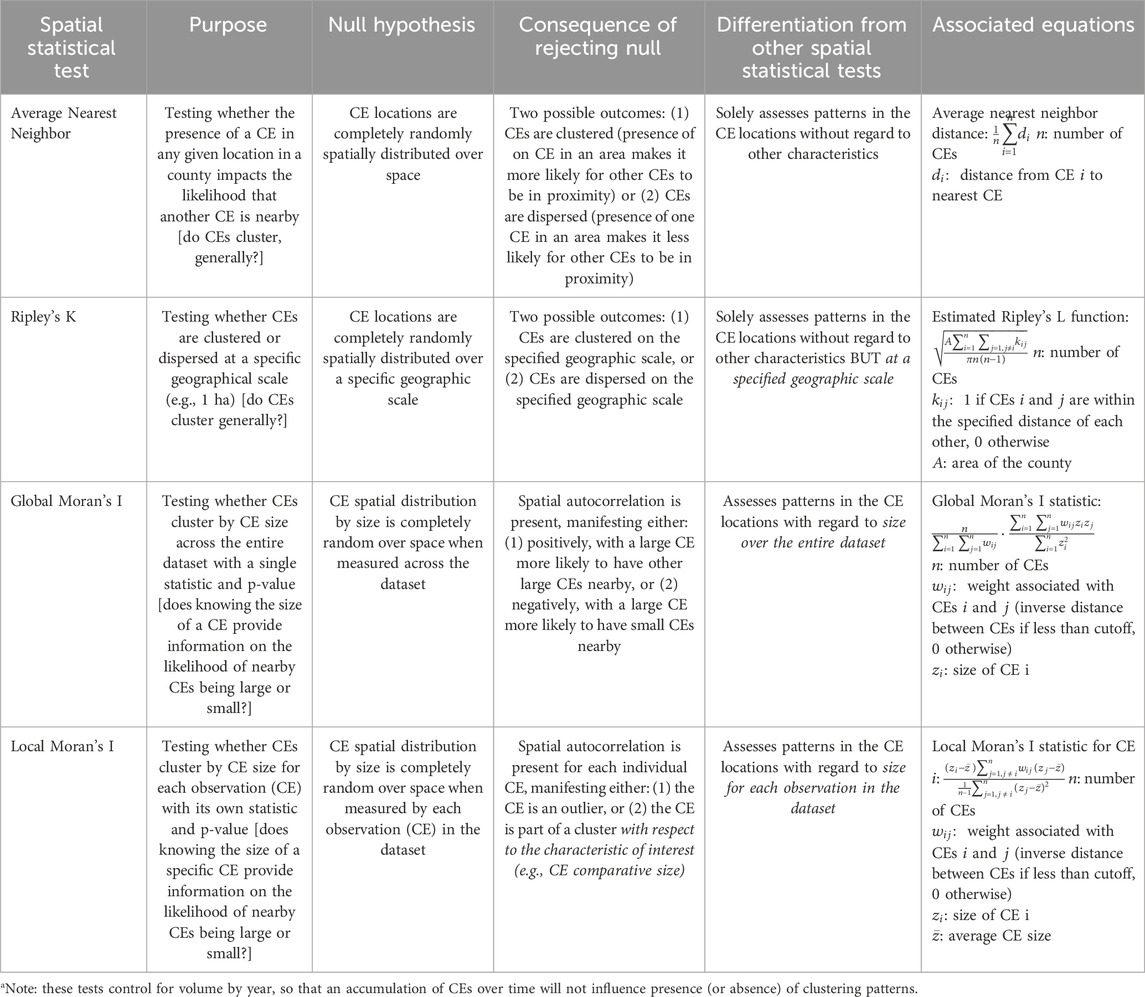
Table 1. Spatial statistical tests employed within a county over time^a.

For Global and Local Moran’s I, we ran the tests on the CE physical size, again with the default settings in ArcGIS (i.e., Euclidean distance for each test). In both of these tests, we used inverse distance weights with no maximum distance, as adjacency-based weights were inappropriate since most CEs are not directly adjacent to other CEs. For the Local Moran’s I test, in the context of CE size, an outlier CE is one whose size is dissimilar to the size of the nearby CEs (e.g., a large CE surrounded by small CEs) and a clustered CE is one whose size is similar to the size of nearby CEs (e.g., a large CE with other large CEs nearby). If the CEs revealed a non-random spatial pattern through these tests, we asked which previous findings and positive theories from the literature might help to explain that spatial pattern. These analyses are inclusive, so there is no independence of years (Supplementary Material). The sheer volume of CEs does not lead to spatial clustering outcomes over time, as the spatial statistical tests control for this possibility.

To examine the potential effects of the 2001 federal tax law change, we subdivided the CEs in each county into those adopted between 1997–2001 and those adopted between 2002–2008/2009 for one set of analysis and subsequently divided the CEs into two other subsets by county: those that had a biological reason enumerated first, and those that did not. For each of these subsamples, we ran the spatial analysis enumerated in Table 1. For the biological analysis, fewer counties had a biological reason as the primary purpose throughout the time frame—and one county, Lebanon, had none.

3 Results

3.1 Basic CE distribution and characteristics

The median years in which CEs were added ranged from 2001 to 2005, with very low coefficient of variation (CV) values, suggesting little dispersion in the years of CE placement in each of the counties (Table 2). All counties had greater than 90% of perpetually restricted CEs. Douglas had the highest percentage of CEs established for a finite, rather than perpetual period (7.81%). Only one county, Washington, had CEs that are generally smaller than 4,046.86 square meters (one acre) (Table 2). Otherwise, the counties could be divided into fairly equal distribution across three tiers: 4,046.86–202,342.82 square meters (one to fifty acres, three counties), 202,343.82–404,685.64 square meters (fifty to one hundred acres, four counties), and 404,686.64–607,028.46 square meters (one hundred to one hundred fifty acres, four counties). There was no discernable geographic trend across these tiers, and no state had two counties in the same tier. The CE holders were notably different depending on the county (Supplementary Figure S1). Land trusts were the predominant CE holders in four counties, while a state entity held the majority in four others (Supplementary Materials). The CE reasons varied in content and number, with a range of 1–16 enumerated reasons per CE. The average reason count was 5.60 (median 6) and 363 (12.6%) CEs had one enumerated reason. Table 2 and Supplementary Table S2 include the first listed reasons by county, which varied across the counties; half have an agriculturally related first reason. In nine counties, we found that CE parcel sizes exceeded median parcel sizes of the same or other land uses in the county. In Greenville, Washington and Douglas, median agricultural parcels were consistently larger than the median CE parcel size (Table 2 and Supplementary Table S3).

Table 2

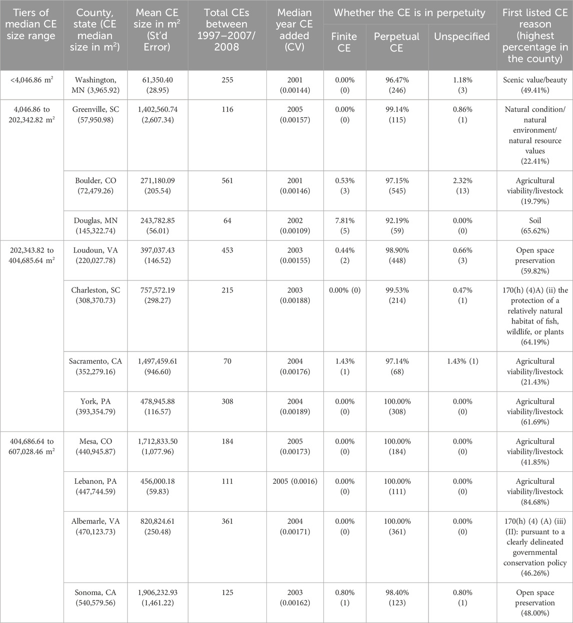
Table 2. Basic CE statistics across the counties.

3.2 Spatial CE patterns

3.2.1 CE clustering by CE area over the entire study period

The Ripley’s K function indicated statistically significant clustering, showing a consistently higher observed value than the expected value over time in each county. The counties are divided into two distinct clustering patterns: near and far significant clustering for most years, as the observed values were higher than the expected values regardless of distance (nine counties); and near significant clustering for all years but either far significant clustering in only a few years or none at all (three counties, Table 3; Figure 1). With a fixed area in each county’s boundary, we ran the ANN tool to calculate the average distance from CE centroid to the other nearest CE centroids by county and over each year. This displayed a consistent clustering trend over time, with CEs in all counties ultimately clustered by 2009 (Table 3). Both global tests that measure whether CEs cluster generally showed that they did so.

Table 3

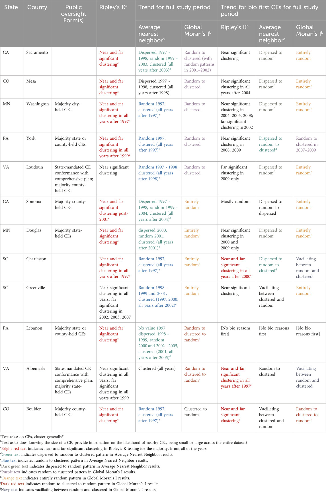
Table 3. Spatial Trends by County for Full Study Period (grouped by the four Global Moran’s I patterns for all CEs).

Figure 1

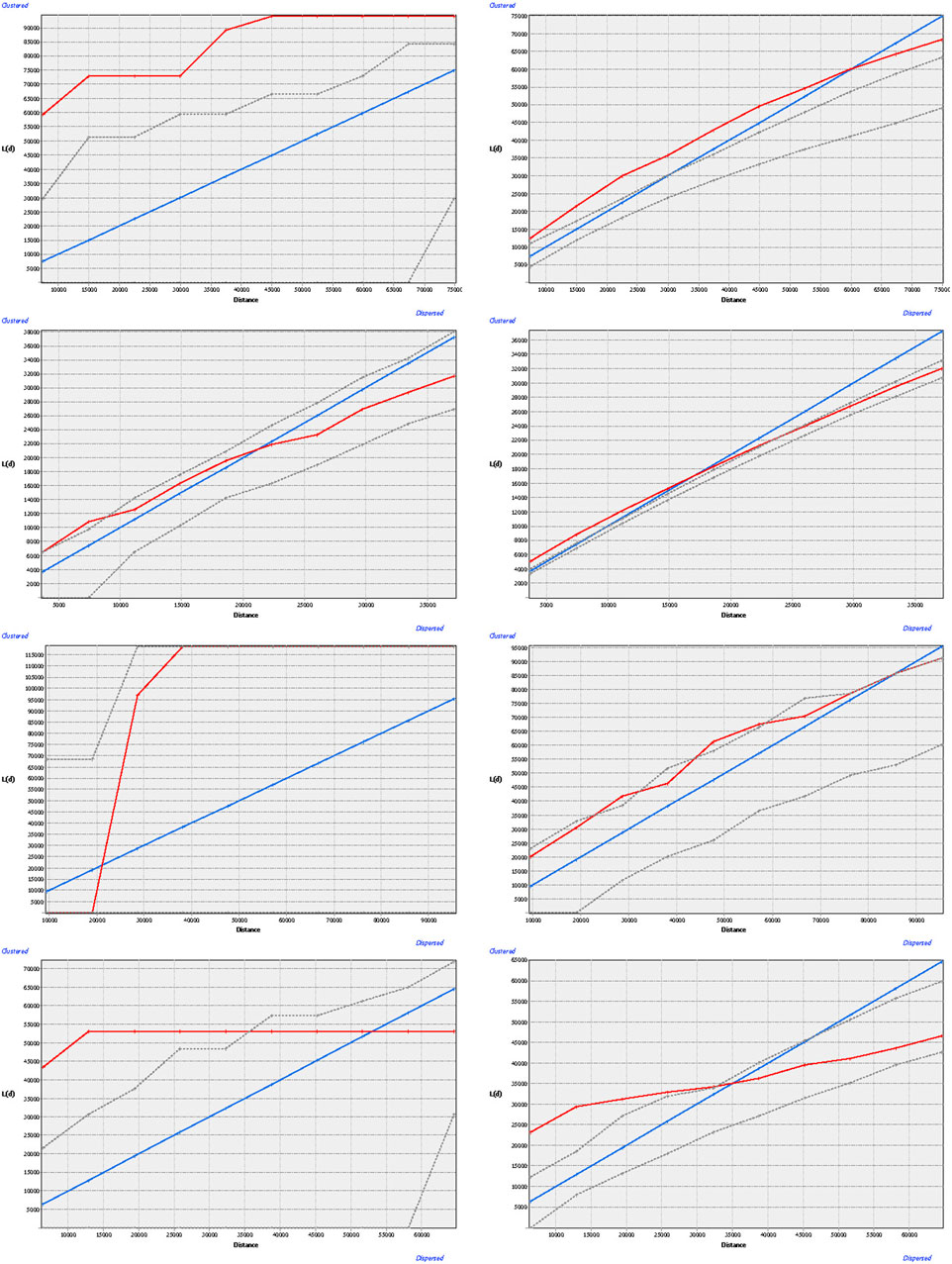
Figure 1. Exemplary Ripley’s K results. The figure depicts examples of the behavior of Ripleys K function under different types of spatial patterns. Sacramento County, California exhibited a random pattern in 1997 (first row left) but near and far significant clustering in 2009 (first row right). Loudon County, Virginia (second row) exhibited near significant clustering in 1997 (right) and 2009 (left). Sonoma County, California (third row) exhibited a random pattern in Bio First CEs in 2003 (right) and a mostly random pattern in Bio First CEs in 2009 (left). Greenville County, South Carolina (fourth row) exhibited significant near clustering in Bio First CBs in 1997 (right) and 2009 (left). In each graph, the $\text{red}$ line indicates the observed K value, the $\text{blue}$ line indicates the expected K value, and the dotted grey lines indicate the confidence envelope.

However, when asking whether CEs tend to be like proximate CEs by size through Global Moran’s I, results revealed an absence of a single pattern across the study counties. Size does not impact adjacent CE size when clustering, or alternatively stated, CE distribution by size is spatially random across these datasets. Most counties started in a random pattern in early years and evolved in four ways. Five counties showed clustering of CEs by size, while CEs remained randomly associated by size in four other counties. Two counties moved from a random to clustered and back to a random pattern. Boulder alone moved from clustered to random. At the end of the study period, when combining the entirely random, clustered to random, and random to clustered to random patterns, most counties (seven) displayed overall spatial randomness in CEs associating with other CEs by size (Table 3).

Local Moran’s I results suggest that smaller CEs are clustered with smaller CEs, while larger CEs are clustered with larger CEs over time. Toward the end of the study period, there are some smaller CEs clustering with a larger CE as well (Table 4; Figures 2, 3). The CE sizes are relative, meaning that there is no threshold for small or large CEs; their size is determined by those in proximity in any given year. Of the clustering and outlier patterns, the low-low (small-small) clustering was volumetrically the largest from 1999–2009 compared to the other forms (followed by high-high clustering, high-low outliers, and low-high outliers). However, it was concentrated in fewer counties (eight of the twelve), while the high-high clustering was present in every county (Table 4; Figure 3). The high-high clustering was the second highest in total count, which was logically lower compared to physically smaller (low-low) clustering since there are likely fewer large CEs in a county. The evolution in high-high (large-large) clustering over the study period manifested consistently across most of the counties except in Albemarle, Greenville, Lebanon, and Sonoma, which had many fewer and more sporadic high-high clusters over time. The low-low clustering and the high-low outlier patterns were present in the early years, and then the high-high clustering emerged quickly while the high-low outliers were comparatively less common. Later years also had a few low-high outliers, particularly in Boulder and York (Table 4).

Table 4

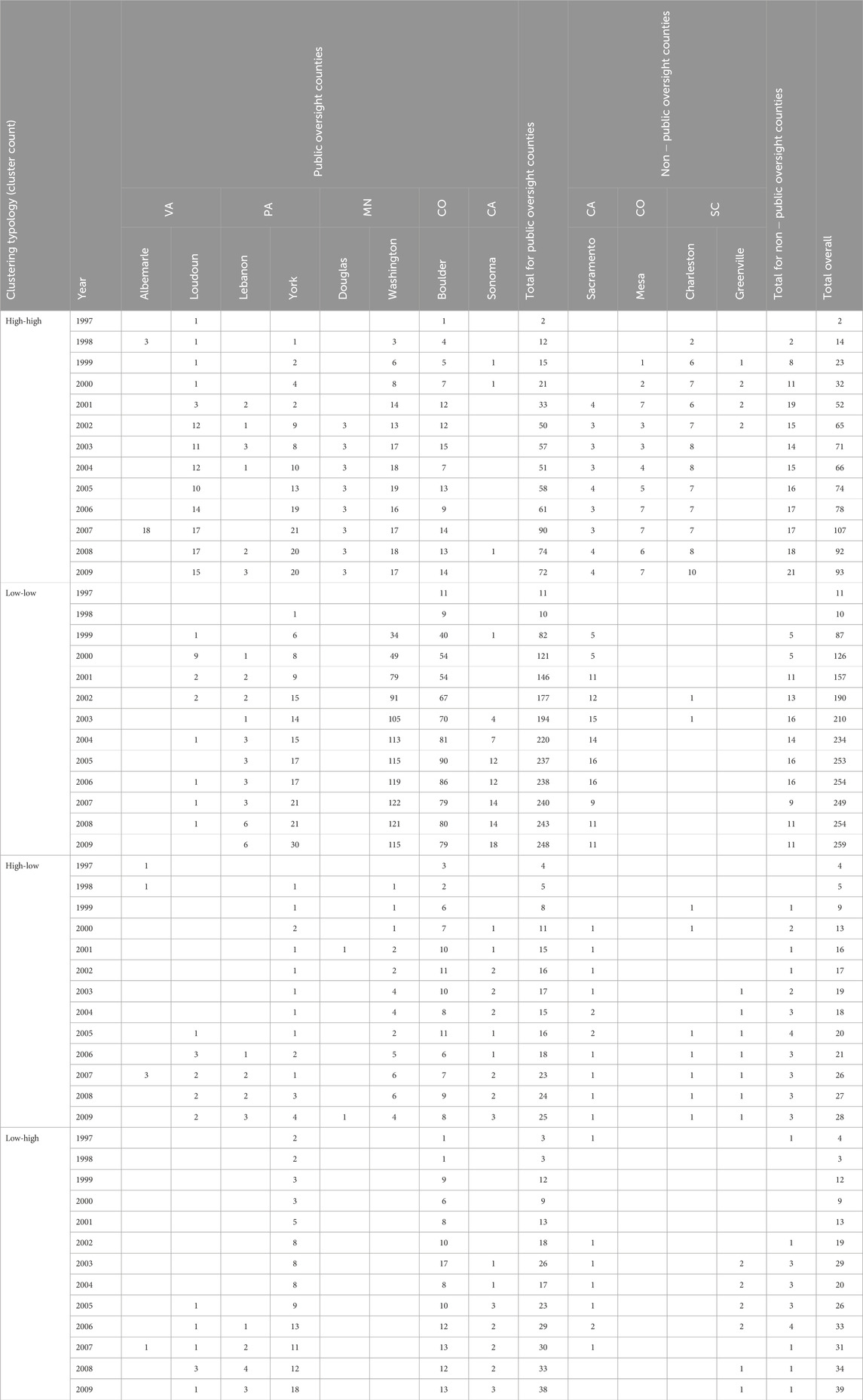
Table 4. Local Moran’s I Clustering for All CEs Over Time (numbers of clusters by year).

Figure 2

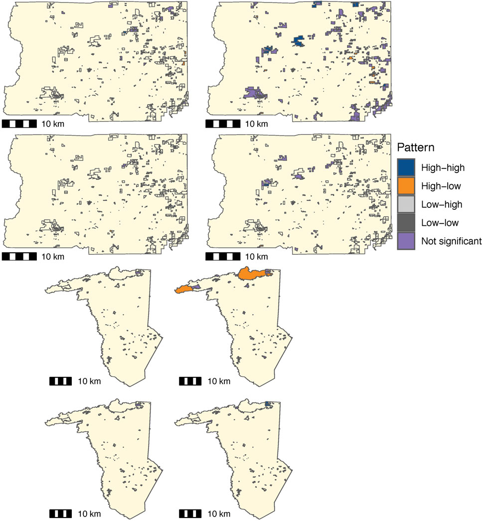
Figure 2. Exemplary Local Moran’s I results. The figure displays the Local Moran's I results for Boulder County, Colorado (top) and Greenville County, South Carolina(bottom) counties. Results for all CEs are shown in rows 1 and 3; results for Bio First CEs are shown in rows 2 and 4. The columns correspond to the years 1997/1998 (left) and 2009 (right). Greenville County, South Carolina had no Bio First CEs in 1997, so results are shown for 1998.

Figure 3

Figure 3. Local Moran’s I clustering typologies.The figure displays the Local Moran's I results for all of the CEs over time in each county.

3.2.2 Public oversight in the CE placement process

The subsample of eight public oversight counties (see Section 2.2) revealed the same Ripley’s K patterns represented in the larger study, with near and far significant CE clustering in a majority (six) of the counties and a smaller pattern of near significant clustering for two counties (Table 3). Similarly, the ANN results moved from a random to a clustered pattern over time. There were four patterns in the Global Moran’s I results over the study period for these counties: random to clustered (three counties), entirely random (two counties), random to clustered to random (two counties), and clustered to random (one county) (Table 3). These results suggest that the spatial distribution of the CEs by size was clustered in only three of the eight counties, with the majority resulting in a random association over time like that of the larger study. In the Local Moran’s I analysis, Boulder was the only county to reveal all types of clustering and outliers by CE size consistently across the entire period. Otherwise, the counties with public oversight do not display a distinct trend in Local Moran’s I clustering typologies, save that the two counties with majority state-held CEs (Albemarle and Douglas) lacked both low-low clustering and low-high outliers (Tables 3, 4). Together, the larger sample of twelve urbanizing counties and the subsample of the public oversight counties display a definite, non-random spatial pattern in the CEs, based—to some extent—on their size if measured by location.

3.2.3 CE clustering pre- and post-tax law change

In both sets of tests asking whether CEs cluster generally (Ripley’s K and ANN), each tax law period showed significant near and far clustering for most of the counties, like the overall study over time. Douglas, Greenville, and Loudoun were the exceptions in the 1997–2001 period, with near significant clustering (Ripley’s K), and Sacramento was an exception in the 2002–2009 period (Ripley’s K displaying near significant clustering). Otherwise, Ripley’s K showed significant clustering at both near and far distances for the rest of the counties in each study period. Distances less than halfway between the minimum and maximum evaluated distance were considered near; distances more than halfway were considered far. The ANN results were slightly more differentiated, with three counties displaying dispersion in 1997–2001 (Douglas, Sacramento, and Sonoma), and nine with significantly clustered CEs. For 2002–2009, ANN testing revealed significant clustering in all counties but Sonoma (Supplementary Table S4). The general CE clustering similarity across two study periods suggests that there is no difference between CE spatial relationships pre-and post the tax law change.

Knowing the size of a CE does appear to provide information about the likelihood of adjacent CE size after the 2001 legal expansion. Pre-2001, there were only three counties that reveal CE clustering by size with the Global Moran’s I analysis for CEs’ size (Boulder, Lebanon, and York). Between 2002 and 2009, the same analysis revealed a definite clustering pattern in the majority (seven) of the counties (Supplementary Table S4). The only counties showing CEs clustered by size in both periods are York and Loudoun, which are in the same state. Boulder was the only county to change from a significantly clustered pattern prior to 2001 to a random one in the second period (2002–2009). The Local Moran’s I clustering in the 1997–2001 period showed low-low clustering dominance in all counties except Sonoma, followed closely by high-high clustering in all counties except Douglas and Sonoma, and the presence of lower volumes of high-low and low-high outliers in seven counties for each (Table 5). For the 2002–2009 period, again, low-low clustering was volumetrically dominant and present in every county, while high-high clustering was second highest and manifested in all but Sonoma (Supplementary Materials).

Table 5

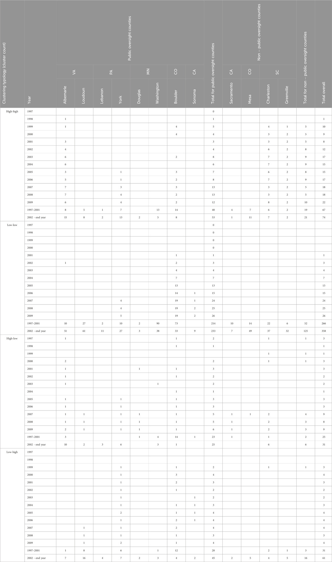
Table 5. Local Moran’s I Clustering for Bio-First CEs and Pre- and Post-2001 CEs (numbers of clusters by year).

The clustering trend by size emerged in both periods, but with greater prevalence and the most definitive difference in the Global Moran’s I results after 2002. When measuring spatial autocorrelation, the CEs exhibit a clustered pattern by size after the tax law change, and both pre-and post-2001, low-low clustering was volumetrically dominant, mirroring the broader study trend in the full 1997–2009 period.

3.2.4 CE clustering by biological reason

Ripley’s K results for the subset of CEs with a biologically related first reason revealed a less uniform pattern than the full study’s distinct trend of near and far clustering (nine counties). The biological CE subset showed near significant clustering for all or most years (three counties), near and/or far significant clustering in select years (four counties), near and far significant clustering for all or most years (three counties), and mostly random (one county) (Table 3). ANN results also showed disparity across the counties over time, with some clustering, some dispersion, and some random CE placement. Some counties moved from dispersed to random to clustered by 2009, while others started out dispersed and moved to random by 2009 (Table 3). Still others moved from random to clustered by 2009, while Sonoma vacillated between dispersed and random over time (Table 3).

The biological CEs’ CE size pattern was variable across the counties, but each county showed clustering, depending on the type of analysis. Global Moran’s I revealed that most the counties’ biological CEs were entirely randomly associated by size over time, except in three counties (Table 3). Local Moran’s I showed high-high clustering over time in five counties, but it lacked consistency by year in the counties where it manifested. Unlike the larger CE population, low-low clustering was present in only four counties, while high-low outliers appeared in different years in nine counties (Table 5; Figure 2). Low-high outliers appeared in five counties over the years (Table 5).

4 Discussion

Using multiple and slightly differentiated spatial tests, our results indicate a non-random spatial distribution of inherently different CEs across physically and socially disparate metropolitan counties experiencing growth pressure, affirming Baldwin and Leonard (2015) and Lamichhane et al. (2021). This trend existed even after the geographic limitation on posthumous donations was lifted in 2001, suggesting that the distance limitation in the posthumously donated CEs may have only slightly influenced their spatial representation (i.e., whether CEs clustered based on size but not whether CEs clustered with other CEs more generally). It appears unrelated to differences in public oversight or whether the CE’s first listed purpose is classified as biological. The Ripley’s K and ANN results suggest that the CEs cluster in most of the counties over time, whether generally or at specific distances.

4.1 CE clustering import for land use optimization

These perpetual CE clusters would impact development potential unless otherwise identified as constraints in spatial optimization and would introduce spatial autocorrelation through neighborhood interaction effects (Grubesic, Wei and Murray, 2014; Irwin and Bockstael, 2004). Solely using Ripley’s K and ANN would lead to the risk of assuming similarity in the CE clusters, but the Global Moran’s I results indicate that CE size impacts clustering, meaning that knowing the size of a particular CE does not necessarily predict a similarly-sized CE in proximity. The Global Moran’s I results showing spatial clustering in five counties present the same spatial autocorrelation issue as the other global tests, but the randomly associated CEs in four counties uphold the assumption that CEs, as “unobserved. . . attributes [,]. . . would not cause estimation problems” in a county-level hazard model (Irwin and Bockstael, 2004, p. 716). Viably determining whether there is global clustering by size is critical to an accurate hazard model.

4.2 CE clustering import for systematic conservation planning

Using both global and local clustering tests overcomes the Global Moran’s I shortcoming of identifying whether—not where—the clustering geographically occurs (Gruebesic, Wei and Murray, 2014). Local Moran’s I results show that CEs are locally spatially clustering based on size in eleven counties. The highest count manifests in smaller CEs clustering with smaller CEs (small CE clustering) in six of the counties, but larger CEs clustering with larger CEs (large CE clustering) are more evenly distributed across almost all counties (Figure 3; Table 4). Counties with small CE clustering may be better positioned to support redundancy with climate change (Carroll and Noss, 2021), depending on their purpose and elevational gradients. Small CE clustering echoes the findings in the Piedmont ecoregion in Lacher et al. (2019), reinforcing emerging conservation biology principles and Whyte’s (1968) suggested CE placement on “in-between lands”.

While logically slightly lower in count, the observable Local Moran’s I trend in large CE clustering over time reinforces the pattern observed in the Blue Ridge (Lacher et al., 2019) and is more prevalent than the small CE clustering across all counties. Large areas of conserved land show that a biologically imperative impact may be present, assuaging climate change-induced land conversion concerns and contravening piecemeal land conservation strategies observed in prior work (Coombes, 2003). Local clustering by CE size—whether in high-high or high-low—is present in every county except Mesa, suggesting the potential for significantly larger land areas to create habitat, regardless of CE purposes (Figure 3; Table 4). Large CE clustering further promulgates the intent of the governmentally mandated 80% open space preservation policy for larger parcels in Irwin and Bockstael’s (2004) hazard modeling for land use optimization and augments spatial optimization to achieve sustainability and prevent sprawl (Yao, Zhang and Murray, 2018).

The biological CE subset is not locally clustering based on size (Table 5), despite some general CE clustering in close distances in the global statistical results (Table 3, Ripley’s K). This means that larger biological CEs are not being placed adjacent to other larger biological CEs to establish buffered and connected areas using the CE instrument (Soule and Noss, 1998). However, the biological CEs are clustering with other biological CEs at finer scales (e.g., a large CE with a few smaller CE parcels, all with biological purposes), possibly ameliorating the size issue, whose import may already be diminishing with climate change (Carroll and Noss, 2021). Non-biological CEs (agricultural and open-space CEs) drive the non-random spatial patterns in the larger population but they can promulgate biological conservation even if they diverge from systematic planning principles (Margules and Pressey, 2000). They may offer remnant and ancillary biological value, manifesting spatial massing for non-biological purposes (Wintle et al., 2019; Brunson and Huntsinger, 2008; Carroll and Noss, 2021).

4.3 CE clustering import for urban planning, open space and climate change

This also suggests that CEs are mitigating urban encroachment on agricultural lands (Vining, Plaut and Bieri, 1977; Hite, Sohngen and Templeton, 2003), impacting urban planning. Land that sustains food production and open space areas are being permanently conserved, supporting urban centers but also limiting developable land supply that can re-direct growth or force densification in existing developed areas. If urban planners are interested in achieving density in urban areas and in maintaining an undeveloped greenbelt/open space network or in controlling leapfrog greenfield subdivisions, they can encourage the use of the CE, particularly in clusters (if they are aware of other CEs, whether through public recording or a more overt public oversight process). The underlying land on which a CE is placed does not have to be biologically valuable to offer a broader public benefit from open space preservation, particularly with the need for climate change refugia. However, the challenge for planners lies in determining a viable mechanism to encourage the property owner to agree to the placement, given the generally perpetual nature of the CE instrument. If the lands are still economically viable, especially in agricultural use, then the property owner may be more inclined to use the instrument. This is where a relationship between land trusts and urban planners may improve the coordination of CE placement, especially in Whyte’s (1968) “in-between lands” where urban planners have less legal influence, but development pressure and property tax increases are mounting. When clustered, the CE can be considered an important element of an open space network.

Our work contributes to the ability to predict preserved open space using a hazard model in rapidly growing areas. Clustering validity—by distance and typology—is integral as an input into the hazard model. If tests such as Ripley’s K, and Global and Local Moran’s I suggest clustering at near but not far distances and only small CE clustering in some counties but large CE clustering across all counties, this will impact the variable input in a hazard model that optimizes land use change with open space preservation requirements per parcel. Landowners are making these CE placement decisions without formal local governmental policy guidance, and these decisions manifest one form of “unobservable attributes of landowners that will generate differences in decisions regarding the optimal timing of conversion”—or limit it entirely if a perpetual CE (Irwin and Bockstael, 2004, p. 716). It is crucial to be able to rely on the spatial clustering tests to reveal whether there is potential for spatially correlated errors that skew the results of the hazard model in predicting the effects of open space preservation.

Our study supplements existing gaps and/or limited geographic scales of previous CE clustering investigation and generates a baseline for future exploration of the revealed patterns (Hennerdal and Nielsen, 2017; Grubesic, Wei and Murray, 2014). We found higher counts of smaller CEs clustering with smaller CEs in some counties, and a pattern of fewer but more consistently present larger CEs clustered with other larger CEs across all counties. Notably, the CEs with a first designated purpose classified as biological did not indicate clustering based on size, but biological CEs are clustering with other biological CEs at closer scales. These results can impact environmental management responses to climate change biome shifts (Carroll and Noss, 2021), particularly in the systematic conservation planning prioritization matrix (Margules and Pressey, 2000).

4.4 Contributions to theories of CE placement impetus

Non-biological CEs appear to drive the clustering patterns, impacting both urban planning and hazard modeling for land use optimization by limiting development potential on Whyte’s (1968) “in-between lands”. As spatial placement of a public good without uniform governmental planning, spatially clustered CEs at different scales (global and local) affect eligibility of land use change in optimization models, spurring or impeding sprawl depending on the size of the clusters (Irwin and Bockstael, 2004). Our results demonstrate the need to carefully choose spatial statistical tests to reliably distinguish spatial CE patterns over time, reinforcing Grubesic, Wei and Murray’s (2014) and Hennerdal and Nielsen’s (2017) multi-scaled approaches to address the MAUP.

4.5 Limitations of our work

Our results need to be tempered by several limitations for which we sought to reasonably control or correct.

There are actions that are beyond the scope of this article, as follows. First, it is challenging to assess the reliability of the first designated purpose of the CE as the basis for the CE typology. We have assumed that the first listed CE reason is the CE’s primary purpose, but acknowledge that without verification from the property owner, we do not have confirmation of their objective for the CE. The land trusts have individualized processes that can be ad hoc and many use boilerplate language in their CE documents. But we looked at the first purpose versus all purposes and have not seen any statistically significant differences between results. Additionally, slightly more than 10% of the CEs have a single purpose, which justifies using the first reason.

Second, with the county as the unit of study, we do not have information about eligible land for feasible CE placement for each year in which a CE was placed. Instead, we indirectly addressed the issue with the median and average parcel sizes for the other parcels by land use in the counties over time to assess comparability. We found that CE parcels are generally larger than the median parcel size for non-CE land use parcels, suggesting a possible bias towards larger parcels for CE eligibility. But we have no way of confirming this bias without additional methods (e.g., interviews with land trusts and counties). We also know that land uses influence one another regardless of jurisdictional boundaries, making the county line an arbitrary one. However, local policies rest at the municipal and county levels, making them viable units of study.

Third, we do not have counts of CEs present prior to 1997 in each county; if a CE was amended during the 1997–2008/2009 period, then we located the original CE placed prior to 1997 but otherwise, we do not have that representation, which could have already impacted development patterns in the counties prior to 1997. With a limited period of study, we may not have fully measured clustering with CEs that were present prior to 1997.

Fourth, the datasets themselves have been compromised by questions about CE recording in some counties, admissions from the county assessor’s offices that some of their data are somewhat suspect (with duplication, inability to explain inconsistencies or elements of their datasets, inability to locate rolls for particular years, etc.), and concerns that the spatial datasets of CEs do not correspond to the recorded CEs in all counties, per Morris and Rissman (2009). We have cleaned and verified repeatedly, seeking to reduce this error. We also acknowledge that there are some multi-part CEs in some counties with the physical distance between parcels that could impact clustering (and its significance).

There are also aspects of our research design that have inherent limitations. For instance, this work was conducted on twelve counties within six states chosen based on specific criteria, so the sample size is extremely small compared to the number of CEs across the country and is possibly biased (i.e., urbanizing areas that face growth pressure). Also, the parcel size is not part of the centroid calculation, meaning that all of the spatial statistics do not control for parcel size. And finally, some counties have higher CE counts or years in which CEs were too low to be sufficient for analysis.

4.6 Suggestions for further work

We recognize that there are gradations of public oversight and other potential factors influencing CE clustering in urbanizing areas that are not fully reflected in this analysis, warranting additional inquiry. Spatial statistics at multiple scales reveal the effect of governance and/or other forces with an objective or plan, supporting the import of the social influence found in Baldwin and Leonard (2015). They also display the effect of aggregated individual land use decision making (Irwin and Bockstael, 2004). The consistent patterns in the Boulder CEs show stronger spatial clustering than the other counties, but a similarly situated county with many county-held CEs (Sonoma) does not exhibit the same. This inconsistency invites further exploration of public oversight gradations, their processes and variations by state and county, and appurtenant factors that may influence CE spatial expression.

We responded to the dominant theories explaining CE clustering, but there are other possible explanations for which we have not controlled and that warrant additional examination. These include the effect of CE holder type, social motivations driving these patterns (Stroman and Kreuter, 2014), complementarity of CE purposes and underlying land uses on those properties, characteristics of CE lands themselves, and the connectivity between conserved lands (both CEs and other conserved lands in each county) in the Graves et al. (2019), Wallace et al. (2008), and Kiesecker et al. (2007) findings. These are within-county statistical nuances that we have yet to explore and intend to do so in future research.

Nevertheless, our results show that private land preservation is a growing response to urban land conversion and CEs are perpetually clustering as a complement to public land conservation, manifesting Whyte’s (1968) vision of their locational utility. Depending on the CE purpose, they may offer a spatial pattern of smaller but redundant clusters that realize climate change resilience and large CEs are amassing, reflecting island biogeography theory (Carroll and Noss, 2021).

Data availability statement

The datasets in this article are not readily available. They will initially be made accessible, where county agreements do not preclude sharing, via a request to the authors. Within a year from publication, the datasets will be made available through a portal at Clemson University. Requests to access the datasets should be directed to CD, Y2R5Y2ttYUBjbGVtc29uLmVkdQ==.

Author contributions

CD: Conceptualization, Data curation, Formal Analysis, Funding acquisition, Investigation, Methodology, Project administration, Supervision, Writing – original draft, Writing – review and editing. SS: Conceptualization, Formal Analysis, Methodology, Visualization, Writing – original draft, Writing – review and editing. ML: Conceptualization, Funding acquisition, Writing – review and editing. DW: Data curation, Funding acquisition, Investigation, Project administration, Writing – review and editing. NF: Data curation, Formal Analysis, Methodology, Writing – review and editing. SO: Data curation, Formal Analysis, Investigation, Writing – review and editing. AO: Data curation, Formal Analysis, Writing – review and editing.

Funding

The author(s) declare that financial support was received for the research and/or publication of this article. This work was supported by the NSF CNH-L program (award no. 1518455) and the NSF Geospatial Sciences Track (award no. BCS-1068906).

Conflict of interest

The authors declare that the research was conducted in the absence of any commercial or financial relationships that could be construed as a potential conflict of interest.

Generative AI statement

The author(s) declare that no Generative AI was used in the creation of this manuscript.

Publisher’s note

All claims expressed in this article are solely those of the authors and do not necessarily represent those of their affiliated organizations, or those of the publisher, the editors and the reviewers. Any product that may be evaluated in this article, or claim that may be made by its manufacturer, is not guaranteed or endorsed by the publisher.

Supplementary material

The Supplementary Material for this article can be found online at: https://www.frontiersin.org/articles/10.3389/fenvs.2025.1575788/full#supplementary-material

References

Arendt, R. G. (1996). Conservation design for subdivisions: a practical guide to creating open space networks. Washington, DC: Island Press.

Google Scholar

Author anonymous, (2025). Uniform conservation easement Act (amended 2007) (US). Available online at: https://www.uniformlaws.org/HigherLogic/System/DownloadDocumentFile.ashx?DocumentFileKey=95e58042-e8d2-2051-1868-617b5d89a7f9andforceDialog=0.

Google Scholar

Baldwin, R. F., and Leonard, P. B. (2015). Interacting social and environmental predictors for the spatial distribution of conservation lands. PLoS One 10 (10), e0140540. doi:10.1371/journal.pone.0140540

PubMed Abstract | CrossRef Full Text | Google Scholar

Brenner, J. C., Lavallato, S., Cherry, M., and Hileman, E. (2013). Land use determines interest in conservation easements among private landowners. Land Use Policy 35, 24–32. doi:10.1016/j.landusepol.2013.03.006

CrossRef Full Text | Google Scholar

Brunson, M. W., and Huntsinger, L. (2008). Ranching as a conservation strategy: can old ranchers save the new west? Rangel. Ecol. and Manag. 61 (2), 137–147. doi:10.2111/07-063.1

CrossRef Full Text | Google Scholar

Carroll, C., and Noss, R. F. (2021). Rewilding in the face of climate change. Conserv. Biol. 35 (1), 155–167. doi:10.1111/cobi.13531

PubMed Abstract | CrossRef Full Text | Google Scholar

Carruthers, J. I., Hepp, S., Knaap, G. J., and Renner, R. N. (2012). The American way of land use: a spatial hazard analysis of changes through time. Int. Regional Sci. Rev. 35 (3), 267–302. doi:10.1177/0160017611401388

CrossRef Full Text | Google Scholar

Circuitscape (2025). Circuitscape open source program. Available online at: https://circuitscape.org/.

Google Scholar

Coombes, B. L. (2003). Ecospatial outcomes of neoliberal planning: habitat management in Auckland Region, New Zealand. Environ. Plan. B Plan. Des. 30 (2), 201–218. doi:10.1068/b12946

CrossRef Full Text | Google Scholar

Dyckman, C. S., Self, S. W., White, D. L., Overby, A. T., Ogletree, S., Fouch, N., et al. (2025). Going with the grain: scalar conservation easement dataset comparison. Landsc. Ecol. 40 (77), 77–17. doi:10.1007/s10980-025-02085-1

CrossRef Full Text | Google Scholar

Ernst, T., and Wallace, G. N. (2008). Characteristics, motivations, and management actions of landowners engaged in private land conservation in Larimer County Colorado. Nat. areas J. 28 (2), 109–120. doi:10.3375/0885-8608(2008)28[109:cmamao]2.0.co;2

CrossRef Full Text | Google Scholar

Farmer, J. R., Knapp, D., Meretsky, V. J., Chancellor, C., and Fischer, B. C. (2011). Motivations influencing the adoption of conservation easements. Conserv. Biol. 25 (4), 827–834. doi:10.1111/j.1523-1739.2011.01686.x

PubMed Abstract | CrossRef Full Text | Google Scholar

Fouch, N., Baldwin, R. F., Gerard, P., Dyckman, C., and Theobald, D. M. (2019). Landscape-level naturalness of conservation easements in a mixed-use matrix. Landsc. Ecol. 34, 1967–1987. doi:10.1007/s10980-019-00867-y

CrossRef Full Text | Google Scholar

Graves, R. A., Williamson, M. A., Belote, R. T., and Brandt, J. S. (2019). Quantifying the contribution of conservation easements to large-landscape conservation. Biol. Conserv. 232, 83–96. doi:10.1016/j.biocon.2019.01.024

CrossRef Full Text | Google Scholar

Groves, C. R., Jensen, D. B., Valutis, L. L., Redford, K. H., Shaffer, M. L., Scott, J. M., et al. (2002). Planning for biodiversity conservation: putting conservation science into practice. BioScience 52 (6), 499–512. doi:10.1641/0006-3568(2002)052[0499:pfbcpc]2.0.co;2

CrossRef Full Text | Google Scholar

Grubesic, T. H., Wei, R., and Murray, A. T. (2014). Spatial clustering overview and comparison: accuracy, sensitivity, and computational expense. Ann. Assoc. Am. Geogr. 104 (6), 1134–1156. doi:10.1080/00045608.2014.958389

CrossRef Full Text | Google Scholar

Hennerdal, P., and Nielsen, M. M. (2017). A multiscalar approach for identifying clusters and segregation patterns that avoids the modifiable areal unit problem. Ann. Am. Assoc. Geogr. 107 (3), 555–574. doi:10.1080/24694452.2016.1261685

CrossRef Full Text | Google Scholar

Hite, D., Sohngen, B., and Templeton, J. (2003). Zoning, development timing, and agricultural land use at the suburban fringe: a competing risks approach. Agric. Resour. Econ. Rev. 32 (1), 145–157. doi:10.1017/s1068280500002562

CrossRef Full Text | Google Scholar

Irwin, E. G., and Bockstael, N. E. (2004). Land use externalities, open space preservation, and urban sprawl. Regional Sci. urban Econ. 34 (6), 705–725. doi:10.1016/j.regsciurbeco.2004.03.002

CrossRef Full Text | Google Scholar

Kiesecker, J. M., Comendant, T., Grandmason, T., Gray, E., Hall, C., Hilsenbeck, R., et al. (2007). Conservation easements in context: a quantitative analysis of their use by the Nature Conservancy. Front. Ecol. Environ. 5 (3), 125–130. doi:10.1890/1540-9295(2007)5[125:ceicaq]2.0.co;2

CrossRef Full Text | Google Scholar

Lacher, I., Akre, T., Mcshea, W. J., and Fergus, C. (2019). Spatial and temporal patterns of public and private land protection within the Blue Ridge and Piedmont ecoregions of the eastern US. Landsc. Urban Plan. 186, 91–102. doi:10.1016/j.landurbplan.2019.02.008

CrossRef Full Text | Google Scholar

Lamichhane, S., Sun, C., Gordon, J. S., Grado, S. C., and Poudel, K. P. (2021). Spatial dependence and determinants of conservation easement adoptions in the United States. J. Environ. Manag. 296, 113164. doi:10.1016/j.jenvman.2021.113164

PubMed Abstract | CrossRef Full Text | Google Scholar

LII (2025). U.S.C.S. §170(h) Qualified conservation contribution (West 2025). Available online at: https://www.law.cornell.edu/uscode/text/26/170 (Acceseed 02, August 2025).

Google Scholar

Lindstrom, C. T. (2008). A tax guide to conservation easements. Washington, DC: Island Press.

Google Scholar

Margules, C. R., and Pressey, R. L. (2000). Systematic conservation planning. Nature 405 (6783), 243–253. doi:10.1038/35012251

PubMed Abstract | CrossRef Full Text | Google Scholar

McLaughlin, N. A. (2017). Uniform conservation easement Act study committee background report, 283. Salt Lake City, Utah: University of Utah College of Law Research Paper. Available online at: https://dc.law.utah.edu/scholarship/119.

Google Scholar

McLaughlin, N. A., and Machlis, M. B. (2008). Protecting the public interest and investment in conservation: a response to professor korngold's critique of conservation easements. Salt Lake City, Utah: Utah L. Rev., 1561.

Google Scholar

McLaughlin, N. A., and Weeks, W. W. (2009). Defense of conservation easements: a response to the End of Perpetuity, 9. Laramie, Wyoming: Wyo. L. Rev., 1.

Google Scholar

Morris, A. W. (2008). Easing conservation? Conservation easements, public accountability and neoliberalism. Geoforum 39, 1215–1227. doi:10.1016/j.geoforum.2006.10.004

CrossRef Full Text | Google Scholar

Morris, A. W., and Rissman, A. R. (2009). Public access to information on private land conservation: tracking conservation easements. Wisc. L. Rev., 1237.

Google Scholar

Olmsted, J. L. (2011). The invisible forest: conservation easement databases and the end of the clandestine conservation of natural lands. Law and Contemp. Probs. 74, 51. Available online at: https://scholarship.law.duke.edu/lcp/vol74/iss4/4.

Google Scholar

Pidot, J. (2011). Conservation easement reform: as Maine goes should the nation follow. Law and Contemp. Probs 74, 1. Available online at: https://scholarship.law.duke.edu/lcp/vol74/iss4/2.

Google Scholar

Public Law 107-16 (2001). Economic growth and tax Relief Act of 2001.

Google Scholar

Richardson, J. J., and Bernard, A. C. (2011). Zoning for conservation easements. Law Contemp. Problems 74 (4), 83–108. Available online at: https://scholarship.law.duke.edu/lcp/vol74/iss4/5.

Google Scholar

Rissman, A. R., Lozier, L., Comendant, T., Kareiva, P., Kiesecker, J. M., Shaw, M. R., et al. (2007). Conservation easements: biodiversity protection and private use. Conserv. Biol. 21 (3), 709–718. doi:10.1111/j.1523-1739.2007.00660.x

PubMed Abstract | CrossRef Full Text | Google Scholar

Self, S., Overby, A., Zgodic, A., White, D., McLain, A., and Dyckman, C. (2023). A hypothesis test for detecting distance-specific clustering and dispersion in areal data. Spat. Stat. 55, 100757. doi:10.1016/j.spasta.2023.100757

PubMed Abstract | CrossRef Full Text | Google Scholar

Soulé, M., and Noss, R. (1998). Rewilding and biodiversity: complementary goals for continental conservation. Wild Earth 8, 18-28.

Google Scholar

Stroman, D. A., and Kreuter, U. P. (2014). Perpetual conservation easements and landowners: evaluating easement knowledge, satisfaction and partner organization relationships. J. Environ. Manag. 146, 284–291. doi:10.1016/j.jenvman.2014.08.007

PubMed Abstract | CrossRef Full Text | Google Scholar

Sundberg, J. O., and Dye, R. F. (2006). Tax and property value effects of conservation easements. Cambridge, MA: Lincoln Institute of Land Policy.

Google Scholar

Theobald, D. M. (2001). Land-use dynamics beyond the American urban fringe. Geogr. Rev. 91 (3), 544–564. doi:10.1111/j.1931-0846.2001.tb00240.x

CrossRef Full Text | Google Scholar

Theobald, D. M. (2013). A general model to quantify ecological integrity for landscape assessments and US application. Landsc. Ecol. 28 (10), 1859–1874. doi:10.1007/s10980-013-9941-6

CrossRef Full Text | Google Scholar

Vining Jr, D. R., Plaut, T., and Bieri, K. (1977). Urban encroachment on prime agricultural land in the United States. Int. Regional Sci. Rev. 2 (2), 143–156. doi:10.1177/016001767700200203

CrossRef Full Text | Google Scholar

Wallace, G. N., Theobald, D. M., Ernst, T., and King, K. (2008). Assessing the ecological and social benefits of private land conservation in Colorado. Conserv. Biol. 22 (2), 284–296. doi:10.1111/j.1523-1739.2008.00895.x

PubMed Abstract | CrossRef Full Text | Google Scholar

Whyte, W. H. (1968). The last landscape. University of Pennsylvania Press.

Google Scholar

Wintle, B. A., Kujala, H., Whitehead, A., Cameron, A., Veloz, S., Kukkala, A., et al. (2019). Global synthesis of conservation studies reveals the importance of small habitat patches for biodiversity. Proc. Natl. Acad. Sci. 116 (3), 909–914. doi:10.1073/pnas.1813051115

PubMed Abstract | CrossRef Full Text | Google Scholar

Yao, J., Zhang, X., and Murray, A. T. (2018). Spatial optimization for land-use allocation: accounting for sustainability concerns. Int. Regional Sci. Rev. 41 (6), 579–600. doi:10.1177/0160017617728551

CrossRef Full Text | Google Scholar