Effects of topographic variables on traffic-related pollutant concentrations: comparison of AERMOD and CAL3QHCR models

Introduction: This study examines the spatial dispersion of traffic-related pollutants (CO, NO_x, and PM₁₀) along a major highway corridor that connects the Eastern Black Sea Region with northern Türkiye. The primary objective is to compare the performance of two atmospheric dispersion models—AERMOD and CAL3QHCR—and to evaluate how topographic variables influence their outputs.

Methods: Dispersion simulations were performed using AERMOD and CAL3QHCR under identical meteorological and traffic input scenarios. Model predictions were compared using Spearman’s rank correlation coefficient and validated against observational data from ten air quality monitoring stations. Fractional Bias (FB) and Normalized Mean Square Error (NMSE) were employed as statistical performance metrics.

Results: Both models estimated higher pollutant concentrations near highways, but AERMOD consistently predicted higher maximum values (CO: 0.78 ppm; NO_x: 1.48 ppm; PM₁₀: 26.59 μg/m³). CAL3QHCR produced lower estimates (CO: 0.20 ppm; NO_x: 0.09 ppm; PM₁₀: 2.70 μg/m³), yet it showed better agreement with observed CO and NO_x concentrations. Correlation analysis indicated strong negative correlations between pollutant levels and elevation (e.g., CO: r = −0.87). Both models captured the spatial decline in concentrations with increasing distance from the road, particularly within the first kilometer.

Discussion: AERMOD was found to overpredict pollutant concentrations, while CAL3QHCR yielded closer estimates for CO and NO_x. However, both models exhibited poor performance in simulating PM₁₀, as indicated by high NMSE values and consistent underestimation. These findings highlight the significance of topography in dispersion modeling and the necessity of model calibration for PM-based assessments.

1 Introduction

Road transportation stands out as one of the primary contributors to outdoor air pollution, particularly in densely populated urban areas, due to the increase in vehicle emissions that pose serious risks to public health. In response to these growing environmental and health concerns, extensive research over the past few decades has focused on evaluating the effectiveness of various emission reduction strategies aimed at improving air quality by mitigating road traffic-related emissions (Soret et al., 2014; Askariyeh et al., 2017; El-Hansali et al., 2021; Nishitateno et al., 2024).

Among the primary causes of road traffic-related air pollution are the usage of fossil fuels, poor fuel quality, and poor vehicle maintenance. Furthermore, non-exhaust emissions, including sources like brakes, tires, and road surface wear, are not currently subject to legal regulation and contribute to air pollution caused by traffic (Khan et al., 2021; Harrison et al., 2021). Due to the significant impact of road traffic on pollution levels, vehicle traffic in urban areas is considered an index for air quality. The fluctuation in both the time and space of vehicular traffic, particularly in urban areas, impacts the pollution level and exacerbates the overall air quality of the environment (Logothetis et al., 2023). According to estimates, a significant majority of the world’s population will reside in urban areas in the future, particularly in close proximity of major highways where traffic congestion can be felt up to 500 m away (Boogaard et al., 2022).

Vehicle emissions consist primarily of pollutants such as carbon monoxide (CO), nitrogen oxides (NO_x), particulate matter (PM), and volatile organic compounds (VOCs). Secondary pollutants like ozone (O₃) are formed through atmospheric reactions involving these primary pollutants (Iqbal et al., 2021). Exposure to these traffic-related pollutants can lead to serious health problems (Bigazzi and Rouleau, 2017). This condition greatly enhances the significance of modeling road pollution. Currently, air quality estimation, which is crucial for human wellbeing, is conducted through dispersion models that rely on mathematical or physical correlations grounded in scientific principles. These models are employed to evaluate the present condition of air quality by utilising diverse data, predict future trends, make essential management choices, evaluate potential health consequences, and trace the probable sources of specific pollution incidents. Air quality dispersion models comprehensively calculate the interplay between emission sources, meteorological conditions, and other environmental elements (Demirarslan et al., 2017; Johnson, 2022; Fateeva and AYu, 2020). Additionally, these models are employed to assess the effects of vehicle emissions (Bai, 2019). Many studies in the literatures have concentrated on the computation of pollutant concentrations associated with traffic and assessing their real-time dispersion. Additionally, these studies have aimed to ascertain the air quality near roadways. Furthermore, there are research investigations that assess the levels of air pollution caused by vehicle emissions in metropolitan areas and devise ecological strategies to mitigate the risks associated with pollution (Crabtree et al., 2009; Samaranayake et al., 2014; Khalid and Ali, 2019; Craig et al., 2020).

Between 2002 and 2023, the number of automobiles in Türkiye grew by almost 207.80%, reaching 26.6 million from 8.6 million (TSI 2023b). The exponential increase in demand for motor vehicles, combined with their excessive use, results in increased traffic emissions, which lead to an increase in air quality in urban areas. Precise simulation of pollutants, particularly near roadways, is crucial for developing sustainable regional transport strategies and mitigating the potential harm caused by hazardous air pollutants (Ma, 2015).

This study examined the dispersion patterns of CO, NO_x, and PM₁₀ pollutants emitted from the road in northern Türkiye, which links the Eastern Black Sea region with other areas. The dispersion were estimated using the American Meteorological Society/Environmental Protection Agency Regulatory Model (AERMOD View 8.9.0) and the California Line Source Model with Queuing and Hotspot Calculation/Refined (CAL3QHCR) programs in CALRoads View 6.2.6.

The main objectives of the research can be outlined as follows: i) Modeling the behavior of road pollutants in the Eastern Black Sea region and determining their impacts on Ordu (ORD), Giresun (GRSN), Trabzon (TRB), Rize (RZ), and Artvin (ART) provinces located on this highway with dispersion maps. ii) Comparison of Air Quality Dispersion Models (AQDM) results. iii) An assessment was conducted to determine the impact of various independent topographic variables (ITV) – Y (latitude), X (longitude), Aspects (ASP), Distance to Road (DR), Elevation (ELEV), Slope (SLP), and Forest Ratio (FR) - on the calculations performed by the model programs utilised in the study area.

The novelty of this study lies in its comprehensive and comparative assessment of two widely applied AQDMs along a topographically complex transportation corridor in Türkiye’s Eastern Black Sea Region. Rather than relying solely on conventional performance metrics, the study systematically investigates how each model responds to independent topographic variables, thereby uncovering model-specific sensitivities to complex terrain features. To explore inter-model consistency, a comparative analysis was performed under uniform input conditions. For each pollutant and sub-region, modeled datasets were randomly partitioned into 30% training and 70% testing subsets, enabling a robust and reproducible evaluation. Spearman’s rank correlation coefficient was used to assess the level of agreement between the models, providing additional insight into their relative performance. Furthermore, model accuracy was evaluated against empirical data obtained from ten air quality monitoring stations using statistical performance indicators—Fractional Bias (FB) and Normalized Mean Square Error (NMSE). Through this dual-layered approach, the study conducts performance analysis both via empirical validation and model sensitivity to spatial-topographic variables. Collectively, these components form a comprehensive and replicable framework for AQDM intercomparison, particularly valuable in geographically and meteorologically complex environments where observational data may be limited.

2 Materials and methods

2.1 Study area

The Eastern Black Sea Region—one of the three subregions of Türkiye’s broader Black Sea Region (Engin et al., 2007)—is characterized by highly rugged terrain, where mountain ranges rise abruptly from the coastline toward the interior (Figure 1). This distinctive geomorphology generates complex meteorological conditions, rendering air pollutant dispersion modeling both essential and methodologically challenging. The region is bounded to the north by the Black Sea and encompasses a densely populated corridor aligned with the 460-km D010 coastal highway, a major transportation axis linking Europe and Asia (Demirarslan and Zeybek, 2021). As of 2022, the region hosts a population of approximately 2.5 million (TSI, 2023a). Elevated traffic volumes—driven by intercity transportation demands and seasonally intensified by agricultural activity—render this corridor a significant hotspot for vehicular emissions, thereby justifying its selection as the focus of this modeling study. To effectively manage the region’s spatial complexity and maintain computational efficiency, the study area was subdivided into eight discrete modeling sub-regions. Each sub-region was independently analyzed to account for local variations in topography, meteorological conditions, and traffic intensity. This stratified approach enhanced both the spatial resolution and the interpretability of the dispersion modeling results.

Figure 1

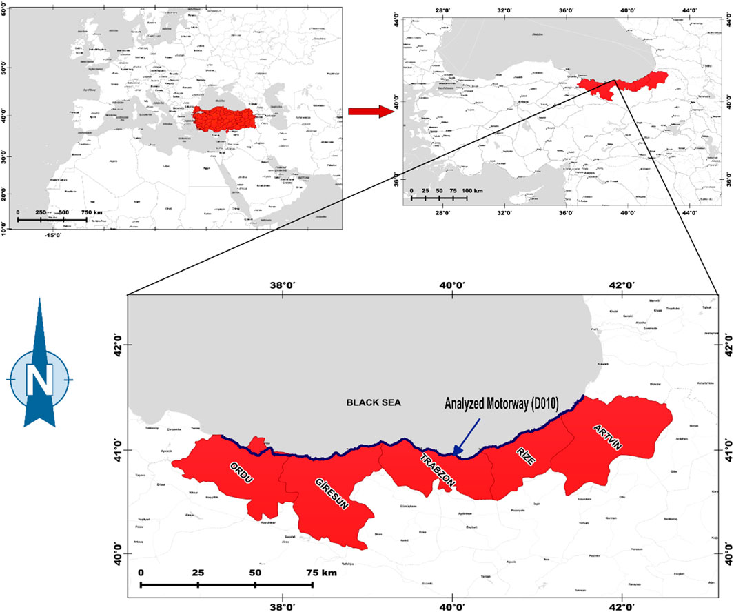
Figure 1. Study area map showing highway network and provincial boundaries used in AQDM simulations.

2.2 Meteorological data

The meteorological data for the study area were obtained from meteorological stations in five provinces. This data is for 2021 and includes variables such as Opaque Cloud Cover (OCC), Dry Bulb Temperature (DBT), Relative Humidity (RH), Station Pressure (SP), Wind Direction (WD), Wind Speed (WS), Ceiling Height (CH), Total Precipitation (TP), Global Horizontal Radiation (GHR), Bowen Ratio (BR), Albedo (A), Planetary Boundary Layers (PBL) and Mixing Height (MH) over a period of 1 year. As both models used in the study required hourly datasets, hourly meteorological data spanning the entire year were utilized. The information about the meteorological stations and the average values of the data obtained are summarised in Table 1.

Table 1

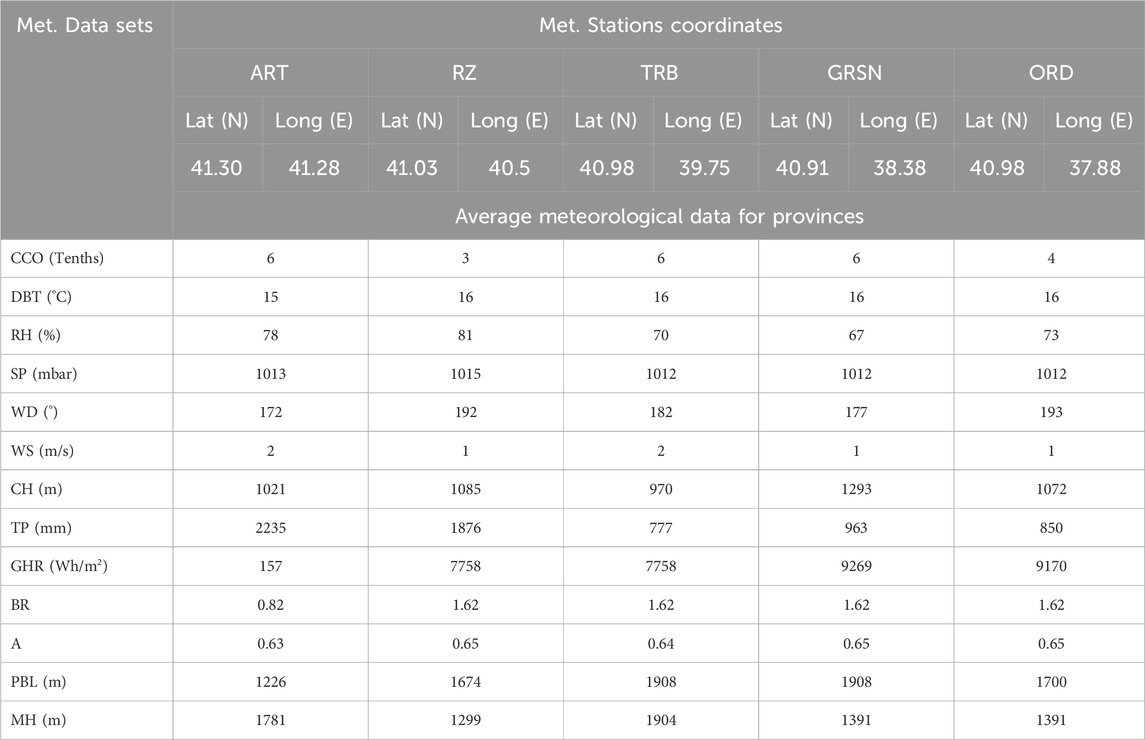
Table 1. Information and mean values of five different meteorological stations in the study area.

The meteorological data utilized in this study were obtained from the Turkish Ministry of Environment, Urbanization, and Climate Change, General Directorate of Meteorology. These data, provided on an hourly basis, were aggregated into annual datasets to ensure consistent inputs for the dispersion modeling process.

The selection of meteorological stations was based on two primary criteria: i) the availability of all necessary input variables compatible with the dispersion models employed in this study, and ii) the spatial representativeness of the stations in covering key locations along the Eastern Black Sea corridor.

Although observational datasets inherently contain potential measurement errors and data gaps, the meteorological data used in this study were sourced from official national monitoring stations operating under standardized protocols. These stations are recognized as reliable sources for air quality modeling applications. Due to the scale and logistical complexity of the study area, conducting independent field measurements was not considered feasible.

For instances where missing data were identified, gap-filling was performed by applying the mean values of the corresponding parameters derived from the same station’s available records. This method was adopted to minimize data discontinuities while preserving the internal consistency and reliability of the dataset.

The emission inventory was developed to characterize traffic-related air pollutants in the study area, with a focus on CO, NO_x, and PM₁₀. In this context, NO_x refers to the combined concentrations of nitric oxide (NO) and nitrogen dioxide (NO₂), reported throughout the manuscript as total NO_x without conversion to NO₂ equivalents. However, a methodological challenge arises during model validation: in Türkiye, national air quality monitoring stations measure only NO₂, as NO_x is not directly monitored. To address this constraint, NO₂ was employed as a proxy for total NO_x. This approach is scientifically justified by the rapid atmospheric interconversion between NO and NO₂ via photochemical reactions, typically occurring within minutes under standard urban daytime conditions (Nowlan et al., 2025). At the emission source, NO constitutes the majority of NO_x emissions (approximately 85%–95%), with NO₂ comprising the remainder (El Abassi et al., 2018; Krol et al., 2024). Due to the rapid oxidation of NO to NO₂, NO₂ concentrations are frequently used as a practical surrogate for total NO_x in urban-scale dispersion modeling and validation. While this introduces a methodological limitation—specifically, the comparison of modeled NO_x with observed NO₂—the use of NO₂ as a proxy remains a widely accepted and scientifically supported practice in the absence of direct NO_x measurements.

The inventory was prepared using the Tier 1 methodology described in the EMEP/EEA Air Pollutant Emission Inventory Guidebook, and the resulting data served as input for dispersion modeling to assess pollutant distribution under regional meteorological and topographic conditions. This approach relies on quantifying the total amount of fuel consumed by vehicles and applying average emission factors to calculate emissions associated with fuel oil usage. Exhaust emissions were then determined based on the general equation presented in Equation 1 (EEA, 2020).

$E_i=\sum _j\left(\sum _m\left(F{C}_{j,m}\times E{F}_{i,j,m}\right)\right)(1)$

In this equation, Ei, emission of pollutant i [g]; FCj,m fuel consumption of vehicle category j using fuel m [kg]; EFi,j,m fuel consumption-specific emission factor of pollutant i for vehicle category j and fuel m [g/kg].

By the end of 2021, the number of registered motor vehicles in Türkiye had reached 25,249,119, with the average age of the national fleet calculated at 14.5 years. When analyzed by vehicle type, the average age was found to be 13.6 years for passenger cars, 15.0 years for minibuses, 14.8 years for buses, 12.8 years for light trucks, and 17.6 years for heavy trucks. Among the 13,706,065 registered passenger cars, 37.6% were diesel-powered, 35.9% used LPG, 25.5% ran on gasoline, and only 0.7% were electric or hybrid vehicles. Vehicles with unspecified fuel types accounted for 0.3% of the total (Turkish Statistical Institute, 2022). These data provide a critical reference for evaluating the emission characteristics of the vehicle fleet in Türkiye. Accordingly, both vehicle types (Passenger Cars–PC, Light Commercial Vehicles–LCV, and Heavy-Duty Vehicles–HDV) and fuel types (gasoline, diesel, and LPG) were explicitly considered in the emission calculations. The primary source of traffic data was the Traffic and Transportation Survey of Highways report for the years 2016–2021, prepared by the Republic of Türkiye Ministry of Transport and Infrastructure, Department of Traffic Safety, Directorate of Transport Studies Branch (TTSH, 2016). However, the report does not provide detailed fleet characteristics such as vehicle age distribution, speed profiles, or driving behavior, which are typically required for more advanced (Tier 2 or Tier 3) emission estimation methodologies.

In the present study, highway traffic passing through eight regions included in the modeling domain was analyzed based on average daily vehicle counts recorded between 2016 and 2021. Traffic data were categorized into three main groups: Passenger Cars (PC), Light Commercial Vehicles (LCV), and Heavy-Duty Vehicles (HDV). The LCV category includes panel vans, small trucks, and pickups, whereas the HDV category comprises trucks, articulated lorries (tractor + trailer), and buses. This classification enabled the application of appropriate emission factors for each vehicle group, thereby improving the accuracy of traffic-related pollution estimates within the modeling framework.

The detailed traffic input data used in both AQDMs are presented in Table 2 (TTSH, 2016).

Table 2

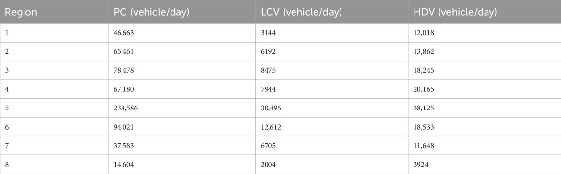
Table 2. Average daily vehicle type distributions for the eight regions within the study area.

In the absence of detailed, site-specific data—such as vehicle age distribution, speed profiles, or driving behavior—Tier 1 emission factors, as defined in the EMEP/EEA Air Pollutant Emission Inventory Guidebook (2019), were adopted in this study. While the Tier 1 methodology involves generalized assumptions, it offers a practical first-order estimation of emissions based on available traffic volume and vehicle classification data. However, the lack of region-specific parameters introduces uncertainties into the modeled outputs. These limitations were taken into account during the evaluation process. The emission factors used for various vehicle–fuel combinations in the calculation of traffic-related emissions are presented in Table 3 (EEA, 2020).

Table 3

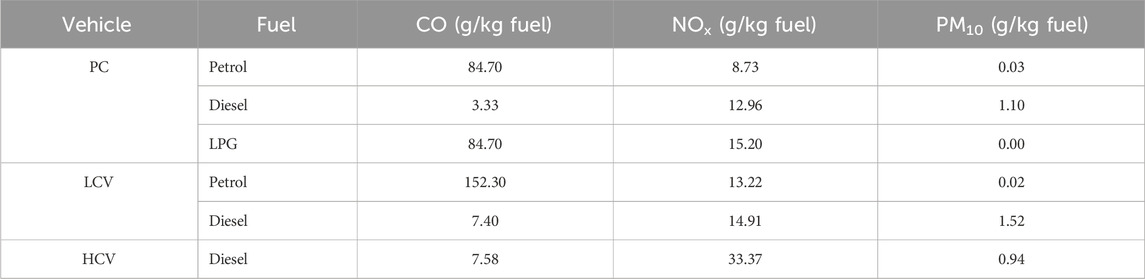
Table 3. Emission factors for Vehicle–Fuel Combinations used in the estimation of traffic-related emissions.

It is important to note that the AERMOD, model requires emission rates to be expressed in grams per second (g/s), while the CAL3QHCR, model utilizes composite emission factors calculated based on vehicle counts and expressed in grams per mile (g/mile), as noted by Zeydan and Öztürk (2021).

2.3 Modeling

This study adopts a dual-modeling framework involving two distinct atmospheric dispersion models: AERMOD and CAL3QHCR. The initial phase employed the AERMOD modeling system to simulate the release and dispersion of inert pollutants in relation to ambient air quality. AERMOD is a steady-state Gaussian plume dispersion model that incorporates boundary layer theory and is applicable to both simple and complex terrain. It is capable of modeling pollutant behavior from various source types—including point, line, and area sources—within a range of up to 50 km. The model also accounts for convective and stable boundary layer dynamics, with horizontal and vertical meteorological parameters determining turbulence structure (Chen et al., 2009; Christopher, 2015; Demirarslan et al., 2017; Bai, 2019; Demirarslan and Yener, 2022).

Meteorological data and emission rates constitute critical inputs in air pollution modeling, significantly influencing the accuracy of simulation results. To generate meteorological inputs for AERMOD, two preprocessors—AERMET and AERMAP—were utilized. AERMET processes observational meteorological data to derive boundary layer parameters, including wind speed, turbulence intensity, and temperature gradients. It requires three input datasets: hourly surface observations, upper-air soundings, and site-specific meteorological measurements (Jamshidi Kalajahi et al., 2019). AERMAP, the terrain preprocessor, provides elevation data for both emission sources and receptor locations, enabling precise terrain characterization (Misra et al., 2013).

The CAL3QHCR model, by contrast, is designed primarily for near-roadway microscale applications and is particularly suited to assessing vehicular emissions. It applies a Gaussian dispersion approach to estimate hourly average pollutant concentrations based on traffic volumes, vehicle speeds, types, and emission factors. The model accounts for crosswind effects and computes pollutant concentrations by integrating emissions from multiple road links. It thereby enables the estimation of pollution contributions from roadway traffic at specific downwind receptor locations (Claggett, 2014; Xiao et al., 2021).

While CAL3QHCR is conventionally applied at localized scales, this study extends its use to a regional corridor spanning approximately 426 km in the Eastern Black Sea region. The objective was to evaluate its comparative performance alongside AERMOD, which is capable of modeling dispersion over both short and long distances. Despite the limitations inherent in extrapolating CAL3QHCR beyond its intended scope, its regulatory acceptance and specificity to traffic emissions justified its inclusion in this broader-scale application.

The choice of AERMOD and CAL3QHCR was also influenced by practical constraints, such as restricted access to more advanced or proprietary models. Both models are extensively documented, widely used in regulatory and academic contexts, and offer an effective balance between computational efficiency and applicability. Their combined use allowed for comprehensive assessment of pollutant dispersion at both regional and localized scales.

To ensure methodological consistency and enable direct comparison, both AQDM systems were provided with identical emission inventories and meteorological datasets, which were standardized into compatible units. The 426-km roadway was uniformly modeled as a linear emission source, and a common receptor grid was applied across the entire modeling domain. The study area was subdivided into eight regions, delineated based on administrative boundaries and topographic variation, to allow for region-specific analysis. Each region included 441 receptor points, evenly spaced and georeferenced to identical coordinates along and adjacent to the roadway segments. This standardized configuration enabled a spatially consistent comparison of model outputs.

In the AERMOD framework, traffic-related emissions were represented using a line-area source approach, which captures both the linear geometry of roadways and the lateral dispersion of emissions across the road surface. To maintain temporal consistency, both models were driven by identical hourly meteorological and emission data, aligned with the input requirements of their respective modeling systems.

CAL3QHCR provides data on gas concentrations calculated in ppm. Therefore, the CO and NO_x concentrations results calculated using the AERMOD programme were converted from µg/m³ to ppm in order to facilitate comparison.

2.4 Statistical analysis

An assessment was conducted to determine the impact of various ITVs—X, Y, ASP, DR, ELEV, SLP, and FR—on the pollutant concentration estimates generated by the model programs used in this study. These variables were derived from high-resolution spatial data sources. Specifically, ELEV, SLP, and ASP were extracted from the Digital Elevation Model (DEM) provided by NASA/METI/AIST (2009) using terrain analysis tools in ArcGIS 10.2 (ESRI, 2014). In order to facilitate their inclusion in statistical analyses, the ASP values were transformed into a continuous Radiation Index (RADIND) using the equation proposed by Bolton et al. (2018), which is also provided in Equation 2.

$RADIND=\frac{1-\mathit{COS}\left(\frac{\pi }{180}\left(ASP-30\right)\right)}{2}(2)$

This index ranged from 0.0 on NNE-facing slopes to 1.0 on SSW-facing slopes, providing a normalized measure of solar radiation exposure for each receptor point.

Spearman correlation analysis was employed to examine the associations between pollutant concentrations and selected variables across the study regions. The strength and direction of these relationships were evaluated to gain insights into the spatial patterns of pollutant dispersion. In addition, the Mann–Whitney U test was conducted to assess whether pollutant concentration distributions differed significantly between the dispersion models applied. All statistical analyses were conducted using SPSS version 18.2.1 (IBM, 2021).

To evaluate the degree of agreement between the AQDM systems in predicting pollutant concentrations, a Spearman correlation analysis was conducted on the outputs of the two models. For each of the eight defined regions, the dataset was randomly divided into a 30% training set and a 70% testing set to enhance robustness and reduce the risk of overfitting.

Spearman’s rank correlation coefficient (ρ) was computed separately for the training and testing subsets in each region. These coefficients were subsequently used to evaluate the consistency of the model predictions and the extent of agreement between the AQDM systems.

The strength of the correlations was interpreted according to Spearman’s rank correlation coefficient (ρ), following the thresholds established by Azman et al. (2025):

Weak: ρ < 0.3.

Moderate: 0.3≤ ρ < 0.5.

Strong: ρ ≥ 0.5.

To maintain consistency and enhance clarity in the presentation of results, all pollutant concentration values were rounded to two decimal places (expressed in parts per million, ppm). For measurements falling below 0.01 ppm, scientific notation (e.g., 2.00e-4 ppm) was employed to retain numerical precision and to prevent misinterpretation as zero.

2.5 Model validation and inter-model comparison strategy

In this study, the predictive performance of two atmospheric dispersion models was systematically evaluated by comparing their modeled pollutant concentrations with observed values obtained from air quality monitoring stations. Annual average concentrations of PM₁₀, NO_x, and CO for the year 2021 were collected from ten monitoring stations distributed across five provinces: ORD (3 stations), GRSN (2 stations), TRB (2 stations), RZ (2 stations), and ART (1 station). For each monitoring station, the nearest receptor point within the model domain was identified, and the corresponding modeled concentrations from both AQDM systems were subsequently extracted for analysis. These observational data were provided by monitoring stations located within the study area and are operated under the authority of the Ministry of Environment, Urbanization, and Climate Change of the Republic of Türkiye.

To quantify the agreement between modeled and observed concentrations, two widely used statistical performance metrics—FB and NMSE—were employed. These indicators were computed separately for each pollutant to evaluate model accuracy and to detect any systematic tendencies toward underestimation or overestimation.

Alongside observational validation, an inter-model comparison was conducted to evaluate the degree of agreement between the AQDM systems’ output predictions. For each pollutant and geographical region, modeled datasets were randomly partitioned into training (30%) and testing (70%) subsets to ensure robustness in the evaluation process. The Spearman rank correlation coefficient (ρ) was then calculated to measure the degree of concordance between the two models, offering additional insight into their relative performance under consistent input conditions.

3 Results

3.1 Analysis of concentration dispersion patterns near highways

The study implemented AQDM to estimate the CO, NO_x, and PM₁₀ concentrations caused by traffic. Subsequently, dispersion maps were generated, as shown in Figures 2–4. Hourly dispersion maps for CO and NO_x, as well as 24-h dispersion maps for PM₁₀, were acquired.

Figure 2

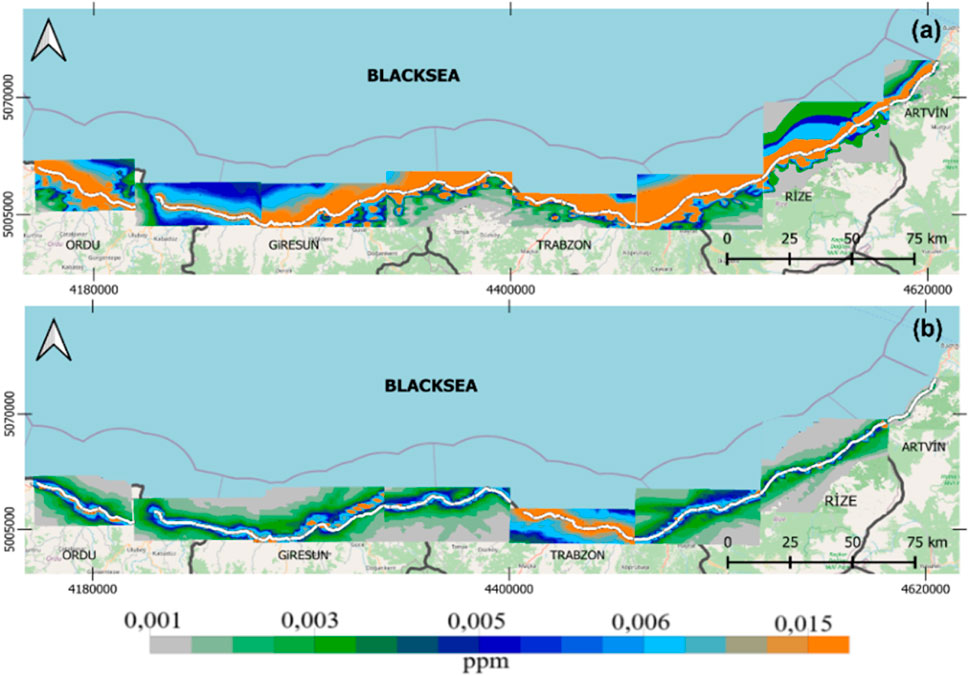
Figure 2. Hourly dispersion maps of CO concentrations [(a) AERMOD, (b) CAL3QHCR].

Figure 3

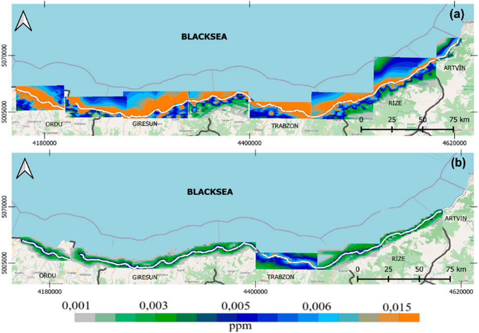
Figure 3. Hourly dispersion maps of NO_x concentrations [(a) AERMOD, (b) CAL3QHCR].

Figure 4

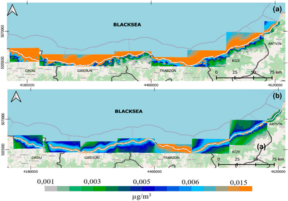
Figure 4. Daily dispersion maps of PM₁₀ concentrations [(a) AERMOD, (b) CAL3QHCR].

Figure 2 illustrates the spatial distribution of hourly CO concentrations along the highway corridor as predicted by AERMOD (a) and CAL3QHCR (b). AERMOD results reveal clearly defined high-concentration zones, particularly in ORD and TRB, where dense urban traffic and complex terrain appear to restrict pollutant dispersion. The model generates narrow, well-aligned plumes along the highway, indicating strong sensitivity to both topographical and meteorological influences.

In contrast, CAL3QHCR produces a more homogeneous distribution with generally lower concentration levels across the study area. The absence of sharply defined peaks suggests that the model may underrepresent pollutant accumulation near highways, potentially leading to more conservative exposure assessments. These differences underscore the structural and parametric contrasts between the two models, particularly in their treatment of near-source dispersion dynamics.

Figure 3 presents the spatial distribution of hourly NO_x concentrations as estimated by AERMOD (a) and CAL3QHCR (b). AERMOD results identify distinct high-concentration zones, especially in ORD and ART, where concentrations reach or exceed 0.015 ppm. The pollutant plumes closely follow the highway alignment, reflecting AERMOD’s ability to capture near-source dispersion behavior under complex coastal topography.

By contrast, CAL3QHCR predicts a smoother distribution pattern with noticeably lower concentration values. The lack of clearly defined hotspots and the gradual gradients suggest reduced sensitivity to localized emissions and dispersion processes. These limitations highlight CAL3QHCR’s structural constraints in representing microscale variations in NO_x concentration.

Overall, AERMOD appears more responsive to highway proximity and urban traffic intensity, making it a more suitable tool for high-resolution NO_x assessments in regions with complex terrain and coastal geography.

Figure 4 depicts the daily dispersion patterns of PM₁₀ as simulated by AERMOD (a) and CAL3QHCR (b). AERMOD results show prominent high-concentration corridors closely aligned with the highway, particularly in ORD and RZ, where urban density and topographic confinement inhibit lateral dispersion. The presence of sharp concentration gradients suggests that AERMOD effectively captures fine-scale pollutant buildup near emission sources.

CAL3QHCR, on the other hand, produces a more diffuse distribution with generally lower concentration levels. Although elevated values are observed in certain areas, such as Giresun and eastern Artvin, the model tends to underrepresent peak accumulation zones. This discrepancy reflects CAL3QHCR’s simplified approach to terrain effects and dispersion mechanisms.

Notably, in comparison to gaseous pollutants such as CO and NO_x, both models predict a broader spatial extent for PM₁₀, consistent with its lower atmospheric reactivity and longer residence time.

3.2 Statistical analyses

3.2.1 Impact of ITVs on concentration dispersion

Statistical analyses were conducted to investigate the relationships between pollutant concentration estimates derived from the AQDM and ITV, focusing specifically on the variables Y, X, RD, ASP, ELEV, SLP, and FR (Table 4). Correlation analysis was employed to assess the patterns of concentration dispersion among these variables and to evaluate their potential interdependencies.

Table 4

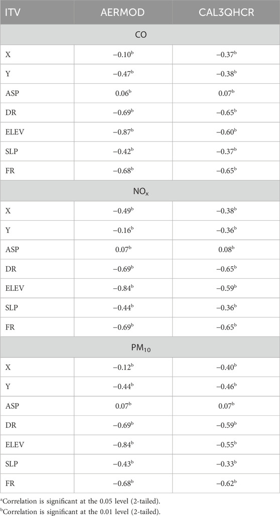
Table 4. Correlation of ITVs with pollutant concentrations estimated by AQDM.

As presented in Table 4, pollutant concentrations estimated by both models exhibit a decreasing trend along the X coordinate, indicating a westward decline. With respect to the Y coordinate, concentrations of CO and PM₁₀ decrease toward the north, and this spatial pattern is consistently supported by both models. The ASP variable shows a weak positive correlation with all pollutants in both models, suggesting that there is no statistically significant relationship between pollutant concentration and slope aspect in the study area. Thus, the influence of ASP can be considered negligible. In contrast, the DR variable demonstrates a strong negative correlation with all pollutants, indicating that pollutant concentrations increase as the distance to the road decreases. This trend is consistently observed in both model outputs. According to the AQDM results, the SLP variable exhibits a moderate negative correlation with pollutant concentrations. This finding implies that sloped terrains may enhance atmospheric circulation, thereby facilitating the dispersion of pollutants. Furthermore, strong negative correlations were observed between the FR variable and pollutant levels in the AQDM model results. This suggests that forested areas contribute to pollutant dispersion by increasing surface roughness and generating structural turbulence.

The correlation analyses among the ITV variables presented in Table 5 provide valuable spatial and environmental insights into the interrelationships of these factors. In particular, the strong positive correlation observed between ELEV and DR suggests that roads are typically located in lower elevation areas, and that both settlement and transportation infrastructure tend to diminish with increasing altitude. Similarly, the high correlation between ELEV and FR indicates that higher elevation zones are more densely covered by forest.

Table 5

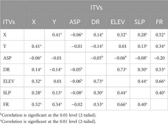
Table 5. Correlations between ITVs.

The positive correlations between DR and both FR and SLP imply that as the distance from roads increases, both slope steepness and forest coverage also tend to increase. This finding suggests that areas with preserved natural landscapes are more likely to be situated in rugged and forested terrains. Additionally, the high correlation between the longitude and FR reveals an increasing trend in forest cover toward the eastern parts of the study area.

On the other hand, the ASP variable exhibited extremely weak or statistically insignificant correlations with all other variables. This result indicates that aspect does not display a systematic association with the other topographic attributes within the study area.

3.2.2 Comparison of AQDMs results

To assess the consistency and predictive accuracy of the two AQDM systems, a comparative analysis was performed using modeled concentrations of CO, NO_x, and PM₁₀. As presented in Table 6, AERMOD consistently estimated higher pollutant concentrations than CAL3QHCR across all statistical metrics (minimum, mean, and maximum), with the most pronounced differences observed for CO and NO_x. In the case of PM₁₀, both models yielded comparable minimum values; however, AERMOD produced substantially higher mean and peak concentrations.

Table 6

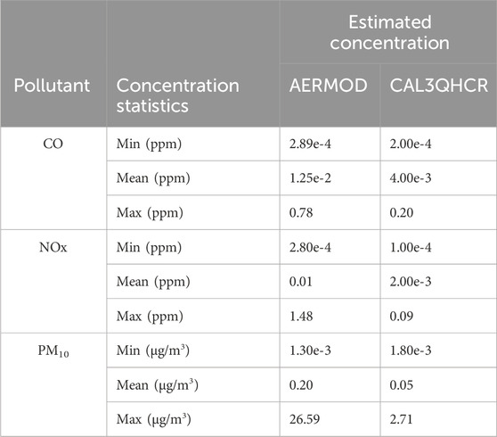
Table 6. Comparative pollutant concentration estimates from AERMOD and CAL3QHCR models.

Statistical significance was evaluated using the Mann–Whitney U test, which revealed significant differences across all pollutants (p < 0.001), indicating that the two models produce markedly different outputs under equivalent input conditions.

The pronounced discrepancy in concentration estimates is likely attributable to fundamental structural differences between the two models. AERMOD’s more advanced representation of atmospheric boundary layer dynamics and terrain influences tends to produce steeper concentration gradients in proximity to emission sources. In contrast, CAL3QHCR, while more conservative in its approach, appears to smooth local variations and underpredict peak values. This divergence is particularly evident in urbanized areas such as ORD and TRB, where AERMOD’s predictions indicate higher pollutant accumulation, likely due to dense traffic and restricted dispersion conditions.

The variations in traffic-related pollutants with distance from the source are presented in tabular form in Tables 7–9. These tables illustrate the trends in pollutant concentrations based on distances from the source in the northern (N) and southern (S) directions for each province.

Table 7

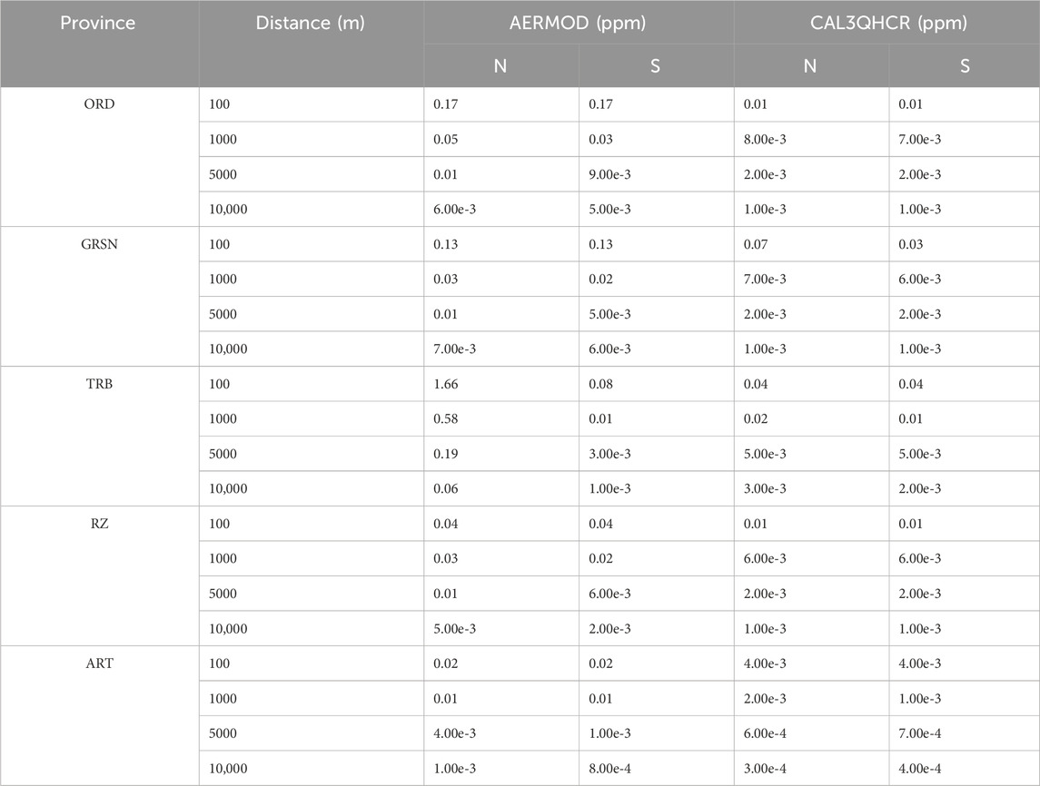
Table 7. Changes in CO concentrations according to distance from the source.

Table 8

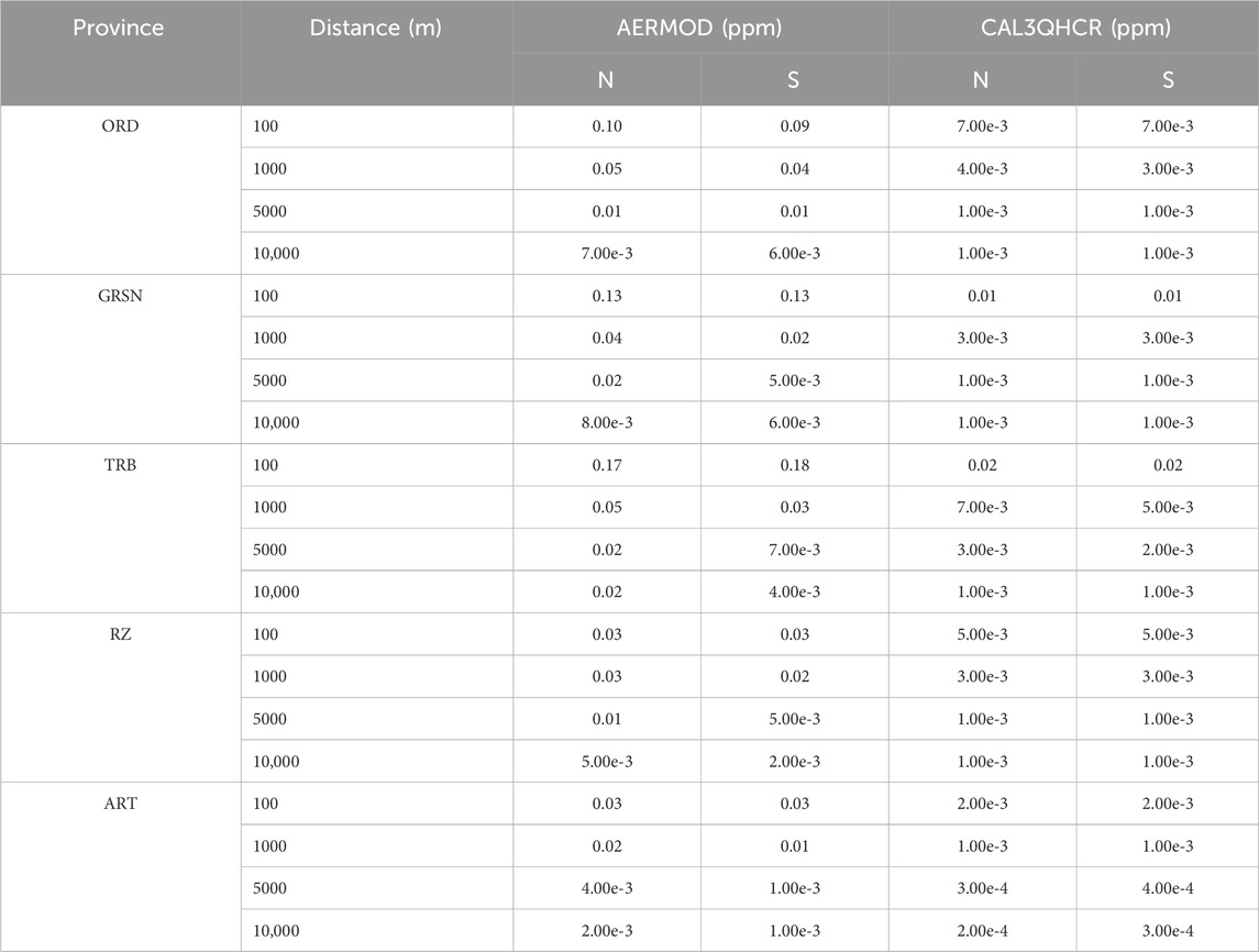
Table 8. Changes in NO_x concentrations according to distance from the source.

Table 9

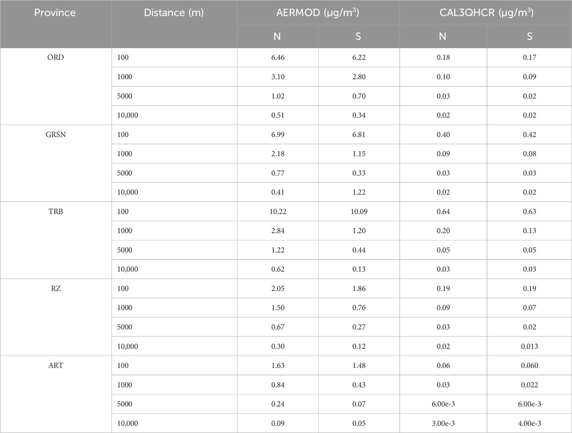
Table 9. Changes in PM₁₀ concentrations according to distance from the source.

As presented in Table 7, CO concentrations consistently decrease with increasing distance from the emission source across all provinces and dispersion models. This pattern is consistent with fundamental atmospheric dispersion principles, driven primarily by dilution and turbulent diffusion. AERMOD consistently predicts higher CO concentrations than CAL3QHCR, particularly within the 100–1000 m range, with the largest discrepancy observed in Trabzon (1.6 ppm vs. 0.04 ppm at 100 m). The steeper concentration gradient observed in AERMOD suggests a greater sensitivity to distance decay, whereas CAL3QHCR displays a more gradual decline. North–South directional differences are minimal in both models, indicating largely symmetric dispersion under the prevailing meteorological conditions.

According to Table 8, NO_x concentrations also decline with increasing distance in both models, aligning with established dispersion theory. Maximum concentrations are observed at 100 m, while the lowest values are recorded at 10,000 m. AERMOD consistently yields higher NO_x estimates than CAL3QHCR, with marked differences within the initial 1000 m. After 5000 m, the concentration predictions from both models begin to converge (approximately 0.001 ppm). The rate of decrease is more pronounced in AERMOD, whereas CAL3QHCR generates comparatively lower and more stable concentration values across distances.

As shown in Table 9, PM₁₀ concentrations diminish with distance from the source in both models, reflecting greater pollutant accumulation near the emission point and reduced levels at greater distances. This trend is more accentuated in AERMOD. Across all locations and distances, AERMOD reports significantly higher PM₁₀ concentrations than CAL3QHCR, with the most substantial differences observed at 100 m. While CAL3QHCR provides lower and more uniform predictions, AERMOD demonstrates a steeper and more variable decline—characterized by rapid reductions at shorter distances and minimal concentrations at longer distances. Although both models exhibit distance-dependent reductions, the rate and magnitude of decline differ substantially between them.

3.2.3 Model comparison and performance evaluation

To assess the degree of agreement between the AQDM systems in predicting traffic-related concentrations of CO, NO_x, and PM₁₀, a Spearman correlation analysis was conducted using the output data from both models. For each of the eight predefined regions, the dataset was randomly partitioned into training and testing subsets to enhance model robustness and mitigate the risk of overfitting. The resulting correlation coefficients for both subsets across all regions are summarized in Table 10.

Table 10

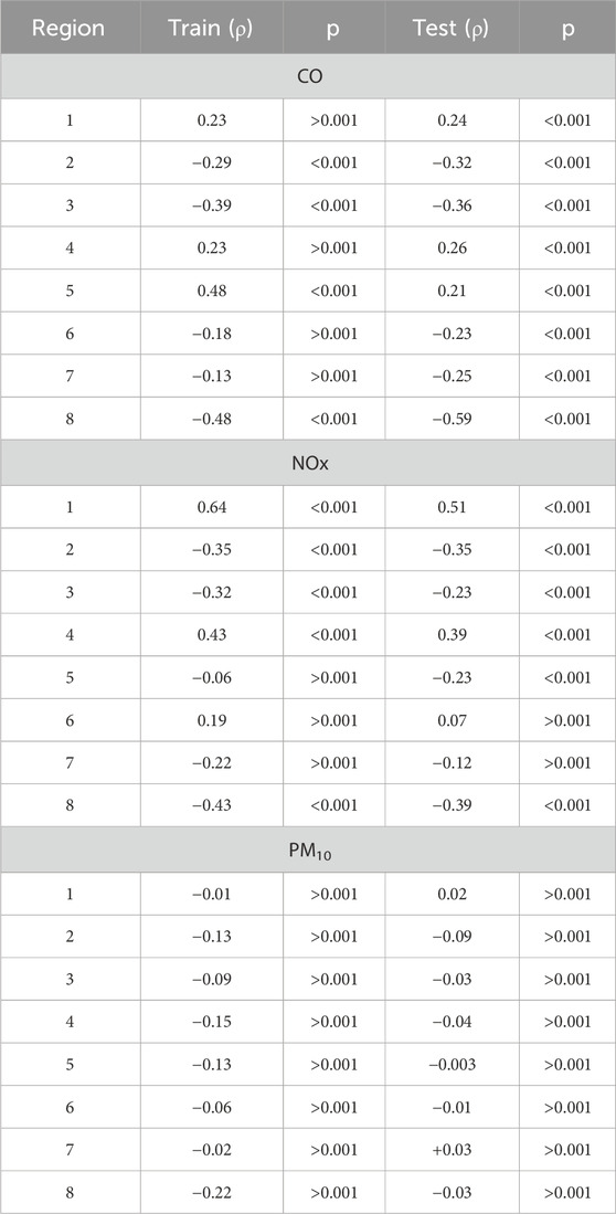
Table 10. Spearman correlation of AQDM model predictions by region and pollutant.

To comprehensively evaluate the predictive performance of the AQDM systems relative to observed concentrations, statistical performance indicators were calculated by comparing the modeled results for the study area with independently measured concentrations of CO, NO_x, and PM₁₀ (Table 11).

Table 11

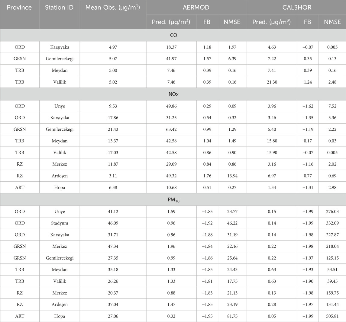
Table 11. FB and NMSE between modeled and observed values for pollutants at monitoring stations in five provinces.

The comparison of AQDM outputs revealed that correlation strength varied in a manner that was both pollutant-specific and region-dependent. For CO, weak positive correlations were observed in Regions 1, 4, and 5, indicating limited agreement. Region 5 showed a moderate correlation in the training set, which declined in the testing set. Conversely, Regions 2, 3, 6, 7, and 8 exhibited negative correlations, with Region 8 displaying a strong and statistically significant negative correlation in the test data. As shown in Table 10, these findings reflect substantial divergence between the models in several regions, likely driven by structural and parametric differences.

For NO_x, model agreement was highest in Region 1 (strong positive correlations) and Region 4 (moderate in both subsets). In contrast, moderate to weak negative correlations were observed in Regions 2, 3, 5, 7, and 8, suggesting systematic prediction differences. Region 6 exhibited only a weak and statistically insignificant correlation, indicating limited alignment.

In the case of PM₁₀, correlations across all regions are consistently weak, with no absolute r value exceeding ±0.3. Additionally, the majority of p-values exceed the 0.05 threshold, indicating an absence of statistically significant relationships. Region 8 constitutes the only exception, where a weak yet statistically significant negative correlation appears in the training set; however, this relationship does not persist in the test subset. Table 10 presents a comprehensive summary of the generally low agreement between the AQDM model outputs in predicting PM₁₀ concentrations. Taken together, the results emphasize that while the models may yield comparable outputs for certain pollutants and regions, they often diverge—particularly in PM₁₀ estimates—highlighting the importance of pollutant-specific and region-sensitive model validation.

The results presented in Table 11 demonstrate that model accuracies vary significantly depending on the pollutant type and monitoring location. The analysis conducted for the CO pollutant indicates that the AERMOD model generally exhibits a systematic tendency to overestimate concentrations, thereby showing a positive bias. In contrast, the CAL3HQR model tends to produce more balanced and observation-aligned predictions. However, it has been observed that the model displays substantial deviations at certain stations, which limits its generalizability. Notably, at the Karşıyaka station, the CAL3HQR model achieved the highest accuracy in CO predictions, as evidenced by its low FB and NMSE values.

In the assessment specific to the NO_x pollutant, the AERMOD model was observed to consistently overestimate concentrations, a trend confirmed by the corresponding FB values. Conversely, the CAL3HQR model generally exhibited a tendency to underestimate, manifesting as a negative bias. The performance of both models varied significantly across stations; for instance, the CAL3HQR model outperformed AERMOD at the Meydan and Valilik stations in the TRB region, as indicated by its lower NMSE values. In contrast, the AERMOD model showed its weakest performance at the Ardeşen station, where it exhibited a particularly high deviation (NMSE: 13.94).

Findings related to the PM₁₀ pollutant reveal that the AERMOD model consistently underestimated concentrations across all monitored stations, exhibiting a pronounced negative bias (FB ≈ −1.85). Although the CAL3HQR model produced predictions closer to observations at certain stations, its high NMSE values suggest uncontrolled variance and low statistical reliability. The model yielded relatively better results at the Meydan and Valilik stations in the TRB region; however, both models demonstrated weak performance at the Hopa, Stadyum, and Ünye stations.

4 Discussion

4.1 Modeling and relationships between emissins and ITV

An examination of the maximum pollutant concentrations predicted by the models reveals that AERMOD consistently estimates significantly higher values than CAL3QHCR, particularly for CO, NO_x, and PM₁₀. For example, in the ORD region, AERMOD predicted a maximum CO concentration of 0.78 ppm and 0.47 ppm in TRB, whereas CAL3QHCR estimated only 0.20 ppm for TRB. Similarly, the highest NO_x concentration predicted by AERMOD was 1.48 ppm, compared to just 0.09 ppm from CAL3QHCR. For PM₁₀, AERMOD projected a maximum concentration of 26.59 μg/m³ in TRB, while CAL3QHCR estimated 2.71 μg/m³.

Despite these differences in magnitude, the spatial distribution of maximum concentrations was similar across both AQDM models, with peaks occurring in comparable coordinate locations. This suggests that both models capture the spatial dispersion patterns of traffic-related emissions in a consistent manner. These findings align with previous research highlighting the substantial contribution of vehicular sources to regional air pollution (Demirarslan and Zeybek, 2021; Tezel et al., 2019; Tezel et al., 2020).

The comparative analysis of AQDM responses to independent topographic variables (ITVs) indicates that both models exhibit broadly consistent dispersion patterns. However, variations in predicted concentration magnitudes arise from differences in their underlying algorithms and their respective treatments of terrain features. Specifically, spatial analyses based on X and Y coordinates reveal a directional decrease in pollutant concentrations from west to east and from south to north. This trend is more pronounced in CAL3QHCR, whereas AERMOD demonstrates weaker sensitivity to these spatial variables, suggesting a more limited capacity to capture directional trends influenced by topographic features. In contrast, the ASP variable showed weak positive correlations with all pollutants in both models, indicating that sun-facing slopes have little influence on pollutant concentrations in the study area.

Other ITVs (DR, SLP, ELEV, and FR) demonstrated moderate to strong negative correlations with pollutant concentrations across both models. These results suggest that these topographic factors promote atmospheric mixing and turbulence, thereby facilitating pollutant dispersion. Notably, AERMOD exhibited greater sensitivity to these variables, likely due to its more detailed parameterization of source–receptor distance, land surface characteristics, and topographic roughness. For instance, the stronger negative correlation observed between DR and pollutant concentrations in AERMOD highlights the model’s enhanced capacity to spatially resolve traffic-related emissions. Similarly, the pronounced negative correlation with FR underscores the role of forested areas in promoting dispersion through increased surface roughness and structural turbulence—an effect to which AERMOD appears particularly responsive.

These results are consistent with previous findings in the literature. For example, Yener and Demirarslan (2022) reported weak negative correlations between PM₁₀ concentrations and X and Y coordinates, as well as varying degrees of correlation between ITV variables and concentrations modeled using AERMOD. Similarly, the strong negative relationship observed between FR and pollutant concentrations aligns with earlier studies highlighting the mitigating effect of forested areas on CO, O₃, and PM₁₀ levels (Baumgardner et al., 2012). The inverse relationship between DR and pollutant concentrations has also been well documented. Numerous studies have shown that pollutant levels—particularly those associated with vehicular traffic—decrease with increasing distance from roadways (Roorda-Knape et al., 1998; Hitchins et al., 2000; Tiitta et al., 2002; Zhu et al., 2002; Gilbert et al., 2003; Zhou and Levy, 2007; Beckerman et al., 2008; Padró-Martínez et al., 2012; Barros et al., 2013; Patton et al., 2014; Pasquier and André, 2017; Huertas et al., 2017). This trend has also been supported by studies employing Gaussian dispersion models, which demonstrate that traffic-related pollutant concentrations decline rapidly with lateral distance from emission sources (Misra et al., 2013). In accordance with this principle, the spatial distribution of pollutants in the present study reveals that the highest concentrations are concentrated along major highway corridors, with levels decreasing sharply as the distance from the highway increases.

Additionally, Claggett (2014) demonstrated that AERMOD tends to predict peak concentrations near roadways, reflecting the tendency of traffic-related pollutants to accumulate in these areas. This observation aligns with the findings of the present study, wherein both models exhibited decreasing pollutant concentrations with increasing distance from the road. However, the rate and magnitude of this decline differed between the models. For example, AERMOD predicted elevated CO concentrations within the first 1000 m, followed by a sharp decline, whereas CAL3QHCR displayed a more gradual and continuous decrease. A similar pattern was observed for PM₁₀: AERMOD showed a steep reduction within the first 500 m, while CAL3QHCR indicated a slower rate of decline.

These differences reflect not only the influence of input parameters but also inherent variations in how each model simulates physical processes such as dispersion dynamics and surface interactions. In this context, the findings of the present study emphasize both the regional influence of ITV variables on air quality and the differing sensitivities of the models to environmental mechanisms. These structural differences should be carefully considered during model selection, as they play a critical role in ensuring the accuracy and reliability of air quality predictions.

4.2 Model comparisons

A comprehensive review of the literature reveals that both AERMOD and CAL3QHCR have been extensively applied to assess the spatial distribution of traffic-related air pollutants, particularly PM₁₀. Zeydan and Öztürk (2021) reported that AERMOD typically produces higher concentration estimates than CAL3QHCR. This difference is largely attributable to AERMOD’s use of advanced dispersion algorithms that more accurately represent atmospheric boundary layer dynamics and complex topographic conditions. In particular, AERMOD’s realistic treatment of local meteorology and terrain results in higher predicted concentrations of CO, NO_x, and PM₁₀—especially under low wind speed conditions (<2 m/s), which are prevalent in the study area.

The observed differences between the two models primarily stem from their structural frameworks and differing levels of environmental sensitivity. AERMOD is a more sophisticated dispersion model, incorporating detailed representations of boundary layer physics and terrain interactions. As a result, it produces outputs that are more responsive to local features such as elevation, slope, and atmospheric stability (Cimorelli et al., 2005). In contrast, CAL3QHCR is a simplified Gaussian line-source model, specifically designed for roadway emissions, with limited capacity to simulate vertical dispersion or account for complex terrain effects (Claggett, 2014).

These structural distinctions help explain why AERMOD demonstrates stronger correlations with topographic variables such as ELEV and SLP. Furthermore, AERMOD relies on preprocessing systems such as AERMET, which enable the model to incorporate site-specific meteorological inputs—e.g., wind direction, speed, and turbulence—more accurately (Tartakovsky et al., 2013). CAL3QHCR, by contrast, typically operates using assumed or simplified meteorological profiles, which may limit its sensitivity to local atmospheric and terrain conditions.

In regions with elevated terrain, pollutants can be transported along sloped surfaces by wind-driven flow, a process that AERMOD simulates with greater detail. Specifically, when terrain elevations exceed stack heights, AERMOD accounts for plume impaction, resulting in higher predicted surface-level concentrations (Carruthers et al., 2011).

When comparing model outputs, AERMOD exhibits stronger correlations with environmental variables such as FR, ELEV, and DR, reflecting its heightened sensitivity to land cover and topographic complexity. In particular, the strong negative correlation between FR and pollutant concentrations supports the hypothesis that forested areas enhance atmospheric dispersion—an effect more accurately captured by AERMOD. Sensitivity analyses by Vallamsundar and Lin (2012) further demonstrate that AERMOD is more responsive to variations in meteorological conditions and source configurations.

However, higher predicted concentrations do not necessarily imply better model performance. Askariyeh et al. (2017) caution that AERMOD’s accuracy may decrease in scenarios involving area sources or highly complex terrain, where increasing elevation can introduce significant prediction errors. Moreover, AERMOD simulations typically require more extensive data inputs and preparation time compared to CAL3QHCR (Vallamsundar, 2014), which may limit its practicality for some applications.

CAL3QHCR, on the other hand, is often favored in regulatory contexts due to its practicality and simplicity in evaluating traffic-related air pollution. Although it does not incorporate high-resolution meteorological inputs or produce time-stamped outputs, it remains a valuable tool for preliminary assessments of roadway emissions (Farzaneh et al., 2017). Craig et al. (2020) observed that CAL3QHCR exhibits higher output variability due to its sensitivity to wind direction, whereas AERMOD generally provides more stable predictions. Nevertheless, AERMOD has been shown to overpredict pollutant concentrations under low wind conditions (<2 m/s), a characteristic meteorological feature of the present study domain.

The findings of this study reaffirm these tendencies. AERMOD consistently produced higher concentration estimates across all pollutants, while CAL3QHCR systematically yielded lower values. This pattern underscores the limitations of relying solely on AERMOD, as it may lead to overestimations, whereas CAL3QHCR’s underestimations pose different challenges, particularly in the context of public health risk assessments and policy formulation. Therefore, understanding the directional biases of both models is essential for informed model selection, interpretation of results, and air quality management decisions.

To better characterize model behavior, comparative analyses were conducted, revealing pollutant- and region-specific variations. For CO and NO_x, the strongest positive correlations between models were observed in Region 1, while statistically significant negative correlations—such as for CO—were identified in Region 8. In contrast, correlations for PM₁₀ were consistently weak and statistically insignificant across all regions, indicating poor inter-model agreement for this pollutant.

To quantitatively evaluate model performance, FB and NMSE metrics were calculated for CO, NO_x, and PM₁₀ at multiple monitoring stations. Results indicated that model accuracy varied by both pollutant type and spatial location. AERMOD generally exhibited a positive bias for CO and NO_x, while CAL3QHCR yielded estimates that were more closely aligned with observed values at certain stations. In contrast, AERMOD significantly underestimated PM₁₀, with FB values ranging from −1.81 to −1.95 and NMSE values reaching 332.08 at the Stadyum station and 505.81 at Hopa, highlighting limitations in its particulate matter predictions.

Although CAL3QHCR produced lower FB values (ranging from 0.05 to 0.63), its NMSE values remained high (125–505), indicating a limited capacity to capture variance despite occasionally matching observed means. Thus, while CAL3QHCR may offer better central estimates under certain conditions, its overall predictive reliability is compromised by its high variability.

Taken together, these findings suggest that AERMOD performs more robustly when applied to comprehensive emission inventories but tends to lose accuracy in traffic-only scenarios, leading to substantial underestimations for certain pollutants. Conversely, while CAL3QHCR may at times align more closely with observed averages, its elevated variance reduces its statistical reliability. These results underscore the importance of pollutant-specific and regionally sensitive model calibration and support the use of hybrid or comparative modeling frameworks to enhance accuracy in urban air quality assessments.

5 Conclusion

This study aimed to model traffic-related air pollutants in Türkiye’s Eastern Black Sea region, generate dispersion maps, and evaluate their impact on local air quality. By applying two widely used atmospheric dispersion models—AERMOD and CAL3QHCR—the research provides critical insights into the spatial variability of pollutant concentrations and the influence of topographic factors in a complex terrain setting.

The analysis of maximum concentration estimates identified Ordu and Trabzon as pollution hotspots for CO, while peak levels of NO_x and PM₁₀ were observed in Trabzon. These findings highlight the city’s elevated traffic density and restrictive topographical features as major contributors to pollutant accumulation.

A central contribution of this study lies in its comparative evaluation of AERMOD and CAL3QHCR. AERMOD consistently predicted higher concentrations, particularly under low wind conditions, whereas CAL3QHCR yielded more conservative and spatially confined estimates. These divergences stem from fundamental differences in model architecture, treatment of meteorological inputs, and sensitivity to terrain resolution. Importantly, neither model proved universally superior. Instead, the results support the adoption of hybrid or context-specific modeling approaches tailored to spatial scale, pollutant type, and policy objectives.

The study also confirmed statistically significant inverse relationships between pollutant concentrations and ITVs—notably ELEV, DR, and FR. Higher FR were consistently associated with lower pollutant levels, reinforcing existing evidence of vegetation’s mitigating role in urban air quality. These outcomes offer empirical support for targeted interventions, such as planting vegetative buffers along transportation corridors and limiting the construction of high-traffic roads in topographically enclosed or densely populated areas.

Looking ahead, the integration of vegetation indices—such as the Enhanced Vegetation Index (EVI) or the Normalized Difference Vegetation Index (NDVI)—alongside high-resolution traffic and land-use datasets, could improve the spatial accuracy of future modeling efforts. Additionally, localized calibration of dispersion models using station-specific air quality measurements would help address persistent over- or underestimation errors, particularly in PM₁₀ predictions.

In conclusion, model selection should be guided not only by data availability and spatial resolution, but also by the intended scientific or regulatory application. AERMOD is better suited for comprehensive, region-wide assessments involving detailed meteorological and emissions data, while CAL3QHCR remains a practical alternative for screening-level and near-roadway analyses. Future research should focus on developing integrated modeling frameworks that combine the strengths of both models, account for terrain complexity, and reflect the dynamic interactions between urban infrastructure and ecological systems.

Data availability statement

The raw data supporting the conclusions of this article will be made available by the authors, without undue reservation.

Author contributions

KD: Data curation, Investigation, Formal analysis, Writing – original draft, Writing – review and editing.

Funding

The author(s) declare that no financial support was received for the research and/or publication of this article.

Acknowledgments

The author is very grateful to the Republic of Türkiye Ministry of Transport and Infrastructure, General Directorate of Highways, for providing traffic and transportation data; to the Republic of Türkiye Ministry of Environment, Urbanization, and Climate Change, General Directorate of Meteorology, for providing meteorological data; and to the same Ministry’s air quality division for supplying air quality monitoring station data within the study area. The author also thanks Dr. İsmet Yener, Faculty Member at Artvin Çoruh University, Faculty of Forestry, for his valuable contribution to the statistical interpretation of the data.

Conflict of interest

The authors declare that the research was conducted in the absence of any commercial or financial relationships that could be construed as a potential conflict of interest.

Generative AI statement

The author(s) declare that no Generative AI was used in the creation of this manuscript.

Publisher’s note

All claims expressed in this article are solely those of the authors and do not necessarily represent those of their affiliated organizations, or those of the publisher, the editors and the reviewers. Any product that may be evaluated in this article, or claim that may be made by its manufacturer, is not guaranteed or endorsed by the publisher.

References

Askariyeh, M. H., Kota, S. H., Vallamsundar, S., Zietsman, J., and Ying, Q. (2017). AERMOD for near-road pollutant dispersion: evaluation of model performance with different emission source representations and low wind options. Transp. Res. Part D Transp. Environ. 57, 392–402. doi:10.1016/j.trd.2017.10.008

CrossRef Full Text | Google Scholar

Azman, M. S. M., Mansor, A. A., Ahmad, A. N., Ismail, M., Jarkoni, M. N. K., and Abdullah, S. (2025). Physio-chemical indoor air quality analysis and CO₂ ventilation forecasting using artificial neural networks in boat manufacturing. Nat. Life Sci. Commun. 24 (1), e2025014. doi:10.12982/nlsc.2025.014

CrossRef Full Text | Google Scholar

Bai, S. (2019). Urban traffic emissions cost estimation using an integrated modeling approach. Montreal: McGill University.

Google Scholar

Barros, N., Fontes, T., Silva, M. P., and Manso, M. C. (2013). How wide should be the adjacent area to an urban motorway to prevent potential health impacts from traffic emissions? Transp. Res. Part A Policy Pract. 50, 113–128. doi:10.1016/j.tra.2013.01.021

CrossRef Full Text | Google Scholar

Baumgardner, D., Varela, S., Escobedo, F. J., Chacalo, A., and Ochoa, C. (2012). The role of a peri-urban forest on air quality improvement in the Mexico City megalopolis. Environ. Pollut. 163, 174–183. doi:10.1016/j.envpol.2011.12.016

PubMed Abstract | CrossRef Full Text | Google Scholar

Beckerman, B., Jerrett, M., Brook, J. R., Verma, D. K., Arain, M. A., and Finkelstein, M. M. (2008). Correlation of nitrogen dioxide with other traffic pollutants near a major expressway. Atmos. Environ. 42, 275–290. doi:10.1016/j.atmosenv.2007.09.042

CrossRef Full Text | Google Scholar

Bigazzi, A. Y., and Rouleau, M. (2017). Can traffic management strategies improve urban air quality? A review of the evidence. J. Transp. and Health 7, 111–124. doi:10.1016/j.jth.2017.08.001

CrossRef Full Text | Google Scholar

Bolton, D. K., White, J. C., Wulder, M. A., Coops, N. C., Hermosilla, T., and Yuan, X. (2018). Updating stand-level forest inventories using airborne laser scanning and Landsat time series data. Int. J. Appl. Earth Obs. Geoinf 66, 174–183. doi:10.1016/j.jag.2017.11.016

CrossRef Full Text | Google Scholar

Boogaard, H., Patton, A. P., Atkinson, R. W., Brook, J. R., Chang, H. H., Crouse, D. L., et al. (2022). Long-term exposure to traffic-related air pollution and selected health outcomes: a systematic review and meta-analysis. Environ. Int. 164, 107262. doi:10.1016/j.envint.2022.107262

PubMed Abstract | CrossRef Full Text | Google Scholar

Carruthers, D. J., Seaton, M. D., McHugh, C. A., Sheng, X., Solazzo, E., and Vanvyve, E. (2011). Comparison of the complex terrain algorithms incorporated into two commonly used local-scale air pollution dispersion models (ADMS and AERMOD) using a hybrid model. J. Air and Waste Manag. Assoc. 61 (11), 1227–1235. doi:10.1080/10473289.2011.609750

PubMed Abstract | CrossRef Full Text | Google Scholar

Chen, H., Bai, S., Eisinger, D., Niemeier, D., and Claggett, M. (2009). Predicting near-road PM2.5 concentrations. Transp. Res. Rec. J. Transp. Res. Board 2123, 26–37. doi:10.3141/2123-04

CrossRef Full Text | Google Scholar

Christopher, W. L. (2015). “Regional scale dispersion modeling and analysis of directly emitted fine particulate matter from mobile source pollutants using AERMOD,” in Doctoral thesis in civil engineering. USA: University Of Californıa.

Google Scholar

Cimorelli, A. J., Perry, S. G., Venkatram, A., Weil, J. C., Paine, R. J., Wilson, R. B., et al. (2005). AERMOD: a dispersion model for industrial source applications. Part I: general model formulation and boundary layer characterization. J. Appl. Meteorology 44 (5), 682–693. doi:10.1175/JAM2227.1

CrossRef Full Text | Google Scholar

Claggett, M. (2014). Comparing predictions from the CAL3QHCR and AERMOD models for highway applications. Transp. Res. Rec. J. Transp. Res. Board 2428, 18–26. doi:10.3141/2428-03

CrossRef Full Text | Google Scholar

Crabtree, B., Dempsey, P., Johnson, I., and Whitehead, M. (2009). The development of an ecological approach to manage the pollution risk from highway runoff. Water Sci. Technol. 59, 549–555. doi:10.2166/wst.2009.876

PubMed Abstract | CrossRef Full Text | Google Scholar

Craig, K. J., Baringer, L. M., Chang, S.-Y., McCarthy, M. C., Bai, S., Seagram, A. F., et al. (2020). Modeled and measured near-road PM2.5 concentrations: Indianapolis and Providence cases. Atmos. Environ. 240, 117775. doi:10.1016/j.atmosenv.2020.117775

CrossRef Full Text | Google Scholar

Demirarslan, K. O., Çetin Doğruparmak, S., and Karademir, A. (2017). Evaluation of three pollutant dispersion models for the environmental assessment of a district in Kocaeli, Turkey. Glob. Nest J. 19, 37–48. doi:10.30955/gnj.001901

CrossRef Full Text | Google Scholar

Demirarslan, K. O., and Yener, İ. (2022). Investigation of total suspended particulate matter dispersion from quarries in Artvin, Turkey, using AERMOD and its relationship with topography. Air Qual. Atmos. and Health 15, 2313–2327. doi:10.1007/s11869-022-01253-5

CrossRef Full Text | Google Scholar

Demirarslan, K. O., and Zeybek, M. (2021). Conventional air pollutant source determination using bivariate polar plot in Black Sea, Turkey. Environ. Dev. Sustain. 24, 2736–2766. doi:10.1007/s10668-021-01553-3

CrossRef Full Text | Google Scholar

EEA (2020). “European environment agency,” in EMEP/EEA air pollutant emission inventory guidebook 2019: technical guidance to prepare national emission inventories (Update Oct. 2020). Available online at: https://unfccc.int/sites/default/files/resource/Manuel%20Copert%205.pdf.

Google Scholar

El Abassi, M., El Haddaj, H., Damich, J., Hanoune, B., and El Maimouni, L. (2018). Evaluation of the NO–NO₂–O₃ photostationary state in roadside environments of Agadir city (southwestern of Morocco). J. Mater. Environ. Sci. 9 (7), 2071–2086.

Google Scholar

El-Hansali, Y., Farrag, S., Yasar, A., Malik, H., Shakshuki, E., and Al-Abri, K. (2021). Assessment of the traffic enforcement strategies impact on emission reduction and air quality. Procedia Comput. Sci. 184, 549–556. doi:10.1016/j.procs.2021.03.068

CrossRef Full Text | Google Scholar

Engin, N., Vural, N., Vural, S., and Sumerkan, M. R. (2007). Climatic effect in the formation of vernacular houses in the Eastern Black Sea region. Build. Environ. 42, 960–969. doi:10.1016/j.buildenv.2005.10.037

CrossRef Full Text | Google Scholar

ESRI (2014). ArcMap 10.2. USA: Redlands.

Google Scholar

Farzaneh, R., Venugopal, M., Pesti, G., Birt, A., Askariyeh, M., Shelton, J., et al. (2017). Air Quality Benefits of Nighttime Construction in Texas Non-attainment Counties — Technical Report. Report No. 0-6864-1.

Google Scholar

Fateeva, Y. G., and Ayu, E. (2020). Data assimilation in modern atmospheric quality forecasting models. 2020 13th international conference “management of large-scale system development” (MLSD). doi:10.1109/mlsd49919.2020.9247717

CrossRef Full Text | Google Scholar

Gilbert, N. L., Woodhouse, S., Stieb, D. M., and Brook, J. R. (2003). Ambient nitrogen dioxide and distance from a major highway. Sci. Total Environ. 312, 43–46. doi:10.1016/s0048-9697(03)00228-6

PubMed Abstract | CrossRef Full Text | Google Scholar

Harrison, R. M., Vu, T. V., Jafar, H., and Shi, Z. (2021). More mileage in reducing urban air pollution from road traffic. Environ. Int. 149, 106329. doi:10.1016/j.envint.2020.106329

PubMed Abstract | CrossRef Full Text | Google Scholar

Hitchins, J., Morawska, L., Wolff, R., and Gilbert, D. (2000). Concentrations of submicrometre particles from vehicle emissions near a major road. Atmos. Environ. 34, 51–59. doi:10.1016/s1352-2310(99)00304-0

CrossRef Full Text | Google Scholar

Huertas, M. E., Huertas, J. I., and Valencia, A. (2017). Vehicular road influence areas. Atmos. Environ. 151, 108–116. doi:10.1016/j.atmosenv.2016.12.006

CrossRef Full Text | Google Scholar

IBM (2021). IBM SPSS Modeler documentation version 18.2. IBMCorp. Available online at: https://www.ibm.com/support/pages/spss-modeler-1821-documentation.

Google Scholar

Iqbal, A., Afroze, S., and Rahman, M. (2021). Probabilistic total PM2.5 emissions from vehicular sources in Australian perspective. Environ. Monit. Assess. 193, 575. doi:10.1007/s10661-021-09352-z

PubMed Abstract | CrossRef Full Text | Google Scholar

Jamshidi Kalajahi, M., Khazini, L., Rashidi, Y., and Zeinali Heris, S. (2019). Development of reduction scenarios based on urban emission estimation and dispersion of exhaust pollutants from light duty public transport: case of tabriz, Iran. Emiss. Control Sci. Technol. 6, 86–104. doi:10.1007/s40825-019-00135-0

CrossRef Full Text | Google Scholar

Johnson, J. B. (2022). An introduction to atmospheric pollutant dispersion modelling. ECAS, 18. doi:10.3390/ecas2022-12826

CrossRef Full Text | Google Scholar

Khalid, L., and Ali, S. (2019). “Dispersion modelling of traffic related pollutants from highways,” in International conference of recent trends in environmental science and engineering. doi:10.11159/rtese19.111

CrossRef Full Text | Google Scholar

Khan, M., Aziz Irfan, M. A., and Ullah, N. (2021). Measurement of traffic-related air pollution in peshawar, Pakistan: a pilot study. Asian Journal of Atmospheric Environment, 15, 78–92. doi:10.5572/ajae.2021.096

CrossRef Full Text | Google Scholar

Krol, M., van Stratum, B., Anglou, I., and Boersma, K. F. (2024). Evaluating NOx stack plume emissions using a high-resolution atmospheric chemistry model and satellite-derived NO₂ columns. Atmos. Chem. Phys. 24, 8243–8262. doi:10.5194/acp-24-8243-2024

CrossRef Full Text | Google Scholar

Logothetis, I., Antonopoulou, C., Zisopoulos, G., Mitsotakis, A., and Grammelis, P. (2023). A case study of air quality and a health index over a port, an urban and a high-traffic location in rhodes city. Air 1, 139–158. doi:10.3390/air1020011

CrossRef Full Text | Google Scholar

Ma, C.-J. (2015). Modeling study on dispersion and scavenging of traffic pollutants at the location near a busy road. Asian Journal of Atmospheric Environment, 9 (4), 272–279. doi:10.5572/ajae.2015.9.4.272

CrossRef Full Text | Google Scholar

Misra, A., Roorda, M. J., and MacLean, H. L. (2013). An integrated modelling approach to estimate urban traffic emissions. Atmos. Environ. 73, 81–91. doi:10.1016/j.atmosenv.2013.03.013

CrossRef Full Text | Google Scholar

NASA/METI/AIST (2009). ASTER global digital elevation model, Japan Space Systems NASA eosdis land processes data.

Google Scholar

Nishitateno, S., Burke, P. J., and Arimura, T. H. (2024). Road traffic flow and air pollution concentrations: evidence from Japan. Int. J. Econ. Policy Stud. 18 (1), 357–385. doi:10.1007/s42495-024-00132-4

CrossRef Full Text | Google Scholar

Nowlan, C. R., González Abad, G., Liu, X., Wang, H., and Chance, K. (2025). TEMPO nitrogen dioxide retrieval algorithm theoretical basis document. Cambridge, MA: NASA Algorithm Publication Tool. doi:10.5067/WX026254FI2U

CrossRef Full Text | Google Scholar

Padró-Martínez, L. T., Patton, A. P., Trull, J. B., Zamore, W., Brugge, D., and Durant, J. L. (2012). Mobile monitoring of particle number concentration and other traffic-related air pollutants in a near-highway neighborhood over the course of a year. Atmos. Environ. 61, 253–264. doi:10.1016/j.atmosenv.2012.06.088

PubMed Abstract | CrossRef Full Text | Google Scholar

Pasquier, A., and André, M. (2017). Considering criteria related to spatial variabilities for the assessment of air pollution from traffic. Transp. Res. Procedia 25, 3354–3369. doi:10.1016/j.trpro.2017.05.210

CrossRef Full Text | Google Scholar

Patton, A. P., Perkins, J., Zamore, W., Levy, J. I., Brugge, D., and Durant, J. L. (2014). Spatial and temporal differences in traffic-related air pollution in three urban neighborhoods near an interstate highway. Atmos. Environ. 99, 309–321. doi:10.1016/j.atmosenv.2014.09.072

PubMed Abstract | CrossRef Full Text | Google Scholar

Roorda-Knape, M. C., Janssen, N. A. H., De Hartog, J. J., Van Vliet, P. H. N., Harssema, H., and Brunekreef, B. (1998). Air pollution from traffic in city districts near major motorways. Atmos. Environ. 32, 1921–1930. doi:10.1016/s1352-2310(97)00496-2

CrossRef Full Text | Google Scholar

Samaranayake, S., Glaser, S., Holstius, D., Monteil, J., Tracton, K., Seto, E., et al. (2014). Real-time estimation of pollution emissions and dispersion from highway traffic. Computer-Aided Civ. Infrastructure Eng. 29, 546–558. doi:10.1111/mice.12078

CrossRef Full Text | Google Scholar

Soret, A., Guevara, M., and Baldasano, J. M. (2014). The potential impacts of electric vehicles on air quality in the urban areas of Barcelona and Madrid (Spain). Atmos. Environ. 99, 51–63. doi:10.1016/j.atmosenv.2014.09.048

CrossRef Full Text | Google Scholar

Tartakovsky, D., Broday, D. M., and Stern, E. (2013). Evaluation of AERMOD and CALPUFF for predicting ambient concentrations of total suspended particulate matter (TSP) emissions from a quarry in complex terrain. Environ. Pollut. 179, 138–145. doi:10.1016/j.envpol.2013.04.023

PubMed Abstract | CrossRef Full Text | Google Scholar

Tezel, M. N., Sari, D., Ozkurt, N., and Keskin, S. S. (2019). Combined NOx and noise pollution from road traffic in Trabzon, Turkey. Sci. Total Environ. 696, 134044. doi:10.1016/j.scitotenv.2019.134044

CrossRef Full Text | Google Scholar

Tezel, M. N., Sari, D., Ozkurt, N., and Keskin, S. S. (2020). Application of reduction scenarios on traffic-related NOx emissions in Trabzon, Turkey. Atmos. Pollut. Res. 11, 2379–2389. doi:10.1016/j.apr.2020.06.014

CrossRef Full Text | Google Scholar

Tiitta, P., Raunemaa, T., Tissari, J., Yli-Tuomi, T., Leskinen, A., Kukkonen, J., et al. (2002). Measurements and modelling of PM2.5 concentrations near a major road in Kuopio, Finland. Atmos. Environ. 36, 4057–4068. doi:10.1016/s1352-2310(02)00309-6

CrossRef Full Text | Google Scholar

TSI (2023a). Turkish statistical Institute, address based population registration system. Available online at: https://biruni.tuik.gov.tr/medas.

Google Scholar

TSI (2023b). Turkish statistical Institute, motor vehicles, january 2023, table-3 number of motor vehicles by years.

Google Scholar

TTSH (2016). Traffic and transportation Survey of highways, traffic safety department directorate of transportation studies branch, general directorate of highways, republic of Türkiye. Ministry Transp. Infrastructure. Available online at: https://www.kgm.gov.tr/sayfalar/kgm/sitetr/trafik/trafikveulasimbilgileri.aspx.

Google Scholar

Turkish Statistical Institute (2022). Motor land vehicles. Available online at: https://data.tuik.gov.tr/Bulten/Index?p=Motorlu-Kara-Tasitlari-Aralik-2021.

Google Scholar

Vallamsundar, S. (2014). Integrated framework for evaluating population health exposure to emissions from transportation sources. Chicago, USA: Graduate College of the University of Illinois at. Thesis of Doctor of Philosophy in Civil Engineering.

Google Scholar

Vallamsundar, S., and Lin, J. (2012). MOVES and AERMOD used forPM2.5 conformity hot spot air quality modeling. Transp. Rec. 2270, 39–48. doi:10.3141/2

CrossRef Full Text | Google Scholar

Xiao, R., Laura, C., and Jason, S. (2021). Air quality assessment kirby road widening city of vaughan. Ontario: Canada. Available online at: https://www.vaughan.ca/projects/transportation/KRW/GeneralDocuments/AppendixR-AirQualityImpactAssessment.pdf.

Google Scholar

Yener, I., and Demirarslan, K. O. (2022). Determining the factors affecting air quality in marmara, Turkey, and assessing it using air quality indices. J. Nat. Hazards Environ. 8 (2), 383–395. doi:10.21324/dacd.1081167

CrossRef Full Text | Google Scholar

Zeydan, Ö., and Öztürk, E. (2021). Modeling of PM10 emissions from motor vehicles at signalized intersections and cumulative model validation. Environ. Monit. Assess. 193, 619. doi:10.1007/s10661-021-09410-6

PubMed Abstract | CrossRef Full Text | Google Scholar

Zhou, Y., and Levy, J. I. (2007). Factors influencing the spatial extent of mobile source air pollution impacts: a meta-analysis. BMC Public Health 7, 89. doi:10.1186/1471-2458-7-89

PubMed Abstract | CrossRef Full Text | Google Scholar

Zhu, Y., Hinds, W. C., Kim, S., Shen, S., and Sioutas, C. (2002). Study of ultrafine particles near a major highway with heavy-duty diesel traffic. Atmos. Environ. 36, 4323–4335. doi:10.1016/s1352-2310(02)00354-0

CrossRef Full Text | Google Scholar