Groundwater estimation and determination of its probable recharge source in the Lower Swat District, Khyber Pakhtunkhwa, Pakistan, using analytical data and multiple machine learning models

This study addresses the lack of integrated hydrogeochemical and machine learning approaches in groundwater assessment, particularly in complex mountainous terrains like the Lower Swat District, Pakistan. It aims to identify recharge sources using a combination of analytical data and advanced machine learning (ML) algorithms. Groundwater recharge sources and demarcation of feasible exploration sites via actual field data and machine learning-based approaches in the Lower Swat District were carried out. Based on variations in subsurface lithological composition (e.g., relative proportions of gravel, clay, silt, and bedrock) and the varying distances of selected well sites from the Swat River, the study area was divided into seven zones. Water samples were collected from surface runoff (river and canals) and groundwater (wells and springs) and analyzed for various physicochemical parameters, including major and trace elements, to identify the probable recharge source in the floodplain area of the Swat River. X-ray fluorescence (XRF) analysis of rock samples collected from the spring hosts was also performed to compare their mineral constituents with the dissolved load of the analyzed groundwater samples. Analytical data interpretation reveals that the recharge source for groundwater in the floodplain regime is the Swat River, while infiltration and percolation of rainwater act as probable recharge sources in the mountainous and elevated areas. Acceptable similarities were observed in the geochemical composition of the rock samples, spring water samples, and representative wells in their immediate neighborhood. A linear relationship was observed between the water table and distance from the Swat River, illustrating that water depth in wells increases with increasing distance from the main recharge source. The study applied six ML models, including random forest, support vector machine (SVM), and ridge Regression, to predict groundwater zones, with random forest achieving the highest accuracy (R² = 0.95, root mean square error (RMSE) = 8.49, and mean absolute error (MAE) = 4.03), followed by decision tree (R² = 0.93). These metrics validate the precision of our groundwater mapping and recharge zone predictions. This integrated approach improves groundwater exploration strategies and supports sustainable water resource management. Furthermore, predicted zones for potential water wells were marked in model wells using artificial intelligence (AI) and machine learning techniques.

1 Introduction

Groundwater is essential for sustainable development and the provision of a steady, renewable supply of drinking water as it provides freshwater to one-third of the world’s population (Carrard et al., 2019; Li et al., 2021). It is primarily recharged through natural processes such as precipitation and the infiltration of river water into aquifers (Zhang and Wang, 2021; Zhang et al., 2023). In Pakistan, the dependency on groundwater is steadily increasing, yet systematic assessments of recharge mechanisms remain scarce, particularly in mountainous terrains like Swat. The improper selection of drilling sites and lack of coordinated exploration often led to ineffective well placement. This study attempts to bridge the gap between geochemical data interpretation and machine learning-based groundwater modeling to offer a replicable framework. However, in urban areas, groundwater resources are increasingly threatened by overexploitation and contamination resulting from industrial activities and unregulated human development, which significantly degrade water quality (Li et al., 2021; Karunanidhi et al., 2022; Akhtar et al., 2021). An additional factor contributing to the significant decrease in aquifer levels is the unrelenting urban demand for water. In order to meet the present water resource demands and supply chain requirements, groundwater exploration using modern hydrological and geophysical techniques is crucial.

The rationale for selecting the Lower Swat District lies in its lithological diversity, unregulated groundwater usage, and increasing population pressure.

Groundwater recharge is the process through which surface water percolates into the earth and replenishes the saturated zone (Boerner and Weaver, 2012). Aquifer recharge can be estimated using a variety of techniques; however, they are primarily dependent on the baseline information that is readily available, including geology, rainfall data, precise topographical information, and climate data across a wide range of temporal and spatial scales. There are several techniques for estimating groundwater recharge, such as groundwater modeling (GM), saturated volume fluctuation (SVF), cumulative rainfall departure (CRD), the extended model for aquifer recharge and moisture (EARTH), water-table fluctuation (WTF), and chloride mass balance (CMB). Among these methods, the CMB method is the most widely used/applied globally to estimate recharge in the aeration and saturation zones (Healy, 2010). According to Marei et al. (2010), due to its conservative nature, the chloride ion is considered to be a good environmental tracer with high solubility in aqueous solutions. Xu and Beekman (2003) concluded that the CMB method is a good technique for recharge estimation in southern Africa after reviewing 30 years of studies on the subject.

Fluctuations in groundwater levels are highly variable in both space and time and are influenced by a number of factors, including geography, climate, and anthropogenic activity (Manna et al., 2019). Although rainfall is often a key driver of groundwater recharge, particularly in shallow unconfined aquifers (Abdullahi and Garba, 2015), human activities such as excessive groundwater extraction for irrigation, urban wastewater infiltration, and land use changes can also significantly influence groundwater dynamics (Ndehedehe et al., 2021; Youssef et al., 2021; Baart et al., 2024). As a conjunctive water management tool, the groundwater table analysis in the spatial–temporal patterns can be used (Vasconcelos et al., 2017). The water-table fluctuation (WTF) method is one of the physical techniques and is based on the idea that groundwater recharge occurs as a result of an increase in the groundwater level caused by earlier rainfall. This method is the most accurate method for estimating groundwater recharge when compared to studies conducted in laboratories to estimate water retention curves and pumping tests (Crosbie et al., 2005). This method is most suitable for calculating groundwater recharge in shallow unconfined aquifers where rainfall has a significant impact on the groundwater level.

With the advancement of remote sensing (RS) and geographic information systems (GIS) over the past few decades, numerous models and algorithms have been developed worldwide (Murasingh et al., 2018; Lee et al., 2018). Different types of lithological and geomorphological units serve as a base for the identification of groundwater potential zones (GWPZs). The integration of RS and GIS is considered to be a flexible tool that increases GWPZ accuracy. Researchers in different regions employ diverse methodologies to ascertain the GWPZs. Certain studies demarcate GWPZs using simple standard mathematical models—for instance, logistic regression (Chen et al., 2018), frequency ratio (Guru et al., 2017; Pourtaghi and Pourghasemi, 2014; Naghibi et al., 2015; Das and Pal, 2019), and weights of evidence (Tahmassebipoor et al., 2016; Chen et al., 2018). However, these necessitate expert-based knowledge, which means that long-term groundwater knowledge is required for the same geo-environmental factor or precise location, which is frequently unavailable. Since the statistical method can map the GWPZ on a scale of 1: 20,000 or 1: 50,000, it can map spring and well locations scientifically (Singh et al., 2013; Jha et al., 2010). However, it disregards non-linear relationships. Thus, a machine learning technique based on AI has been developed. Previous studies on groundwater prediction can broadly be categorized into (i) analytical methods such as chloride mass balance and water table fluctuation, (ii) remote sensing and GIS-based spatial models, and (iii) data-driven machine learning models. Our study builds on the third category, integrating it with geochemical data for enhanced reliability. Despite numerous studies on groundwater recharge and potential zone mapping, few have integrated field-based chemical analysis with multiple machine learning (ML) algorithms in high-grade metamorphic regions like Lower Swat. This study addresses that gap by combining geochemical compatibility analysis and model-based well prediction.

The ML technique relies on data mining, which is necessary for enhancing groundwater capacity (Naghibi and Pourghasemi, 2015; Rahmati et al., 2016; Naghibi et al., 2016; Golkarian et al., 2018; Arabameri et al., 2019). Most studies that evaluate GWPZ use techniques like classification and regression trees (CART) (Naghibi et al., 2015; 2016; Kordestani et al., 2019), random forest (RF) (Youssef et al., 2016; Naghibi and Dashtpagerdi, 2017a; Kim et al., 2018), support vector machines (SVMs) (Naghibi and Dashtpagerdi, 2017a; Lee et al., 2018), and artificial neural networks (ANNs) (Lee et al., 2018). These techniques provide an accurate estimation of a region’s potential for groundwater in the future (Naghibi and Pourghasemi, 2015; Chen et al., 2018). Complex classification and mapping issues are resolved through the use of hybrid machine learning techniques. This method is more effective than a single method because it addresses the shortcomings of individual models (Naghibi et al., 2017b; Kordestani et al., 2019). Researchers propose to design and evaluate new techniques for mapping the groundwater potential zone based on this integrated or hybrid model. Based on the recent literature emphasizing data-driven groundwater potential mapping (Naghibi et al., 2017b; Lee et al., 2018), the present study employs a hybrid AI/ML modeling framework for enhanced predictive accuracy. The reviewed methods directly informed our choice of regression-based and ensemble learning models.

Recent studies have extended the use of machine learning in hydrological assessments. For example, groundwater source identification through unsupervised ML in New Mexico (Hobbs et al., 2025) provides a model for our recharge source detection approach. Similarly, the impact of the Chamravattam regulator on Bharathapuzha River (Ajith and James, 2016) exemplifies the regional hydrological influence of man-made structures. The objectives of this study are (i) to determine groundwater recharge sources using chemical and lithological data; (ii) to apply and compare ML models for well site prediction; and (iii) to evaluate the relationship between geochemistry and distance from the recharge source. Despite extensive studies on groundwater estimation, few have explored the integration of machine learning algorithms with geochemical field data in high-relief terrains. This lack of interdisciplinary methodology limits the reliability of groundwater zone predictions.

2 Materials and methods

2.1 Study area

The study area lies in the Lesser Himalayas, an integral part of the Himalayan Tectonostratigraphic Basin, which is tectonically active and hydrogeologically diverse. The Lesser Himalayas are bounded in the south by a regional tectonic boundary, Main Boundary Thrust (MBT), and in the north by Main Mantle Thrust (MMT), offering a unique combination of metamorphic rocks, igneous intrusions, and unconsolidated glacial and fluvial deposits. The MBT is the southernmost thrust, which places meta-sedimentary rocks of the Lesser Himalayas over the unmetamorphosed clastic rocks of the Himalayan foredeep (Figure 1).

Figure 1

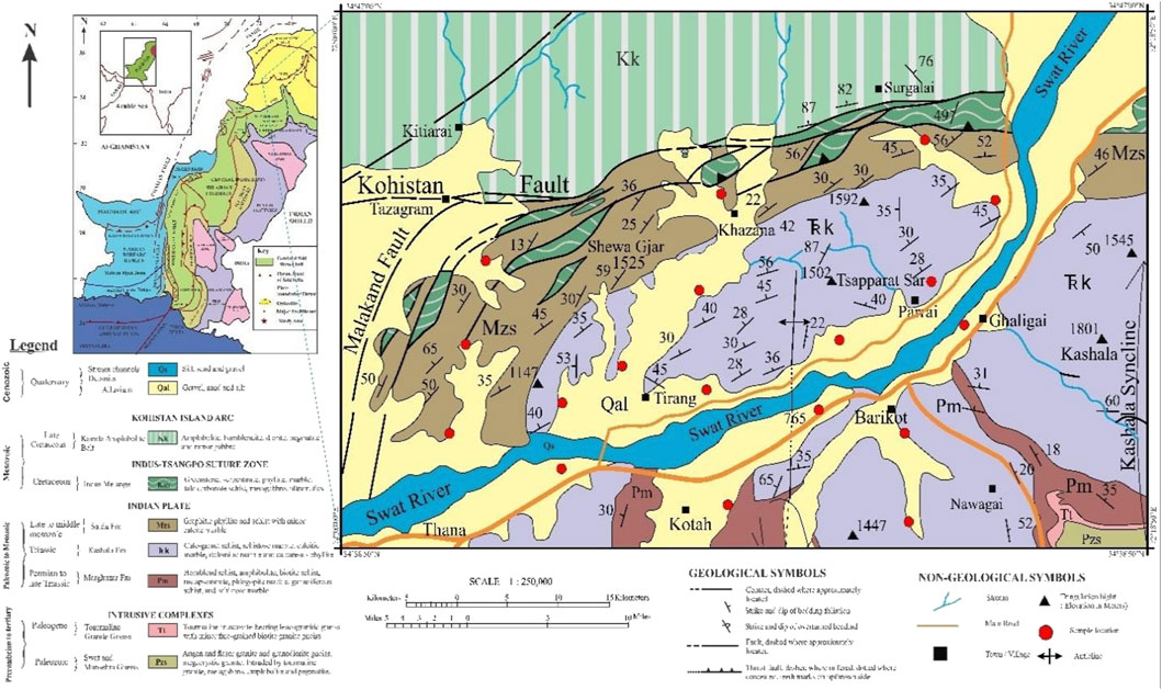
Figure 1. Sampling location map exhibiting geological and tectonic setup of the studied area (modified after Hussain et al., 2014).

Swat District, located in the Lesser Himalayas, is a mountainous terrain composed mainly of metamorphic rocks intruded by several igneous intrusions. Intermontane basins of the study area are filled with unsorted glacial and sorted fluvial deposits. Glacial deposits have capped most of the bedrock units in the Upper Swat District, while fluvial deposits are common in the Lower Swat District. Fluvial deposits are mostly composed of sorted layers of boulders, pebbles, cobbles, sand, silt, and clay. These materials are eroded and transported by multiple perennial and seasonal contributory channels originating from the surrounding mountains. The coarse alluvial deposits comprising sand, gravel, pebbles, and boulders are found along mountain fronts (Figures 2, 3).

Figure 2

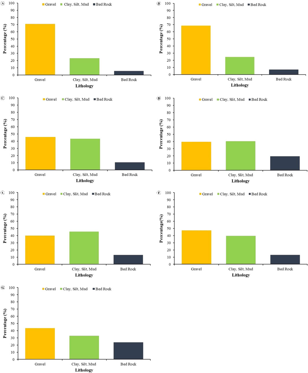
Figure 2. Lithological variations in the well logs of (A) representative wells of Group A, (B) representative wells of Group B, (C) representative wells of Group C, (D) representative wells of Group D, (E) representative wells of Group E, (F) representative wells of Group F and (G) representative well of Group G, during field investigation.

Figure 3

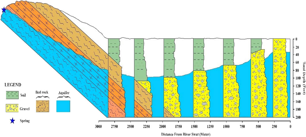
Figure 3. Cross-sectional view of representative wells in the studied area illustrates the depth of water in each well and its distance from the Swat River. Lithological variations of each well represent the host sediments for groundwater accumulation.

The study area was selected due to its increasing reliance on groundwater for domestic and agricultural purposes, increasing urban demand, and lack of systematic groundwater assessments. Its hydrogeological complexity, characterized by varied lithologies and dynamic recharge patterns, makes it an ideal case for assessing groundwater potential and quality. The area’s significance also stems from the presence of multiple perennial and seasonal tributaries that influence sediment distribution and aquifer characteristics, offering valuable insights into groundwater dynamics in mountainous terrains.

2.2 Field survey and sample collection

Extensive fieldwork activity was conducted to collect field data and rock/water samples and mark the inspected area on a map. During this field visit, data including well depth, water level, location, well logs, distance from the Swat River, variations in the water level, and the diameter of the wells (whether they are bore wells or dug wells) from approximately 500 points were collected. Maximum data were acquired through structured interviews with well owners/local residents and field observations. Additionally, the installation dates and the current status of wells along with fluctuations in the water table were also recorded as a basic part of the data collection process. These diverse data points provide a comprehensive overview of the wells in the area, enabling us to analyze and draw meaningful conclusions about the water resources and their associated hydrogeological characteristics.

After an extensive field visit, a total of 15 water samples were collected from various locations and sources (the river, canals, springs, hand pumps, boreholes, open wells, dug wells, and water-logged areas) within the study area and subsequently analyzed (Figure 1). The area was divided into seven zones based on the distance of samples from the Swat River, namely, Group A (0–250 m), Group B (251–500 m), Group C (501–1,000 m), Group D (1,001–1,500 m), Group E (1501-2000 m), Group F (2001–2,500 m), and Group G (2,501–3,000 m). In order to ensure representative sampling, 1–2 samples from each zone were collected. This approach allowed for a diverse range of water sources to be included in the analysis, providing a comprehensive understanding of the water quality and characteristics in the study area.

Sampling locations were selected to reflect spatial heterogeneity in terms of altitude, proximity to surface water bodies, lithological differences, and land use. This strategy aligns with established groundwater sampling guidelines, ensuring comprehensive spatial coverage (APHA, 2017).

Water samples were collected using sterilized polyethylene bottles, labeled properly, and transported within 24 h to the Pakistan Council of Research in Water Resources (PCRWR) laboratory for analysis.

Additionally, four rock samples were specifically collected from the vicinity of springs and wells to complement the water sampling and provide valuable insights into the geological composition and context of the surrounding areas. The rock samples were analyzed at the Centralized Resource Laboratory (CRL), University of Peshawar.

2.3 Sample analysis

The physicochemical characteristics of the water samples, including alkalinity, hardness, total dissolved solids (TDS), carbonates, bicarbonates, calcium (Ca), magnesium (Mg), chloride (Cl), potassium (K), sodium (Na), sulfate (S), and nitrate (N), were determined using standard procedures (APHA, 2017).

The elemental composition (both major elements, i.e., Mg, Ca, Fe, and Si, and minor/trace element, i.e., Mn within the rock samples) of rock samples was analyzed using X-ray fluorescence (XRF) spectroscopy. First, the rock samples were crushed into powder using a crushing machine; afterward, 0.5 g of powdered samples was digested in an aqua regia solution (HNO₃: HCl in a 1:3 ratio) on a hot plate at 200°C for 2 h. After complete digestion, samples were diluted to 100 mL with deionized water, mixed well, and filtered. The major and trace elements including aluminum (Al), silicon (Si), calcium (Ca), iron (Fe), potassium (K), titanium (Ti), sulfur (S), strontium (Sr), zirconium (Zr), vanadium (V), zinc (Zn), copper (Cu), iridium (Ir), and yttrium (Y) in the digested samples were analyzed through XRF.

2.4 Machine learning

ML is a branch of artificial intelligence (AI) that primarily focuses on creating algorithms and statistical models that enable systems to learn from data and make decisions without being explicitly programmed. Huge amounts of data can be used by ML systems for finding patterns, predicting outcomes, or improving performance through experience over time (Domingos, 2012). This technology has made possible the automation of complex processes in several industries, facilitating decision making and generating insights that were hitherto impossible (Jordan and Mitchell, 2015). The heart of machine learning is to create models that generalize well from training data to unseen examples, thus enabling accurate prediction or classification (McAfee and Brynjolfsson, 2017). Various techniques such as supervised learning, unsupervised learning, and reinforcement learning are employed for this purpose in different situations (Bishop, 2006). Machine learning technologies have been expanding their capabilities due to the exponential growth of data and increased computing speed, resulting in innovations such as condition monitoring tools in the healthcare industry; fraud detection algorithms in the financial sector; personalized product development based on customer preferences in marketing; and autonomous navigation systems in drones, among other applications within these fields (Goodfellow et al., 2016). Recent studies continue to show innovative uses of AI/ML in hydrology. For instance, lean construction AI in Iran (Ugural et al., 2024), groundwater potential zone mapping in Kohat (Faheem et al., 2023), and GIS-based recharge studies in Swat (Hussain et al., 2022) support the relevance of hybrid geospatial and machine learning approaches.

2.4.1 Linear regression

Linear regression is a technique in statistics that explains the relation between the dependent variable and one or more independent variables. It is meant to identify the linear equation that best forecasts the dependent variable from other independent variables. The mathematical expression of a simple linear regression line is given by $y=\beta 0+\beta 1x+ϵ$, where y represents the dependent variable, x represents the independent variable, β0 is the y-intercept, β1 denotes the slope of the line, and ε represents the error term, which accounts for variability in y that cannot be explained by its linear relationship with x. The parameters β0 and β1 are estimated using methods such as the least squares procedure, which minimizes the sum of squared differences between the observed values and those predicted by the model (Weisberg et al., 2013; Seber and Lee, 2012).

2.4.2 Decision tree

The decision tree is a flexible machine learning model that can be used for classification and regression. It splits data into subsets based on input features recursively to form a tree-like structure, with each node representing a decision made based on a feature and each leaf node standing for the predicted outcome. The objective in regression is to make predictions about continuous dependent variable $y$ using one or more independent variables $x_1,x_2,\dots ,x_p$. Usually, the splitting criterion at each node is the mean squared error (MSE), which is calculated as shown in Equation 1:

$\text{MSE}\left(t\right)=\frac{1}{N_t}{\displaystyle \sum _{i\in t}}{\left(y_i-\widehat{y_t}\right)}^2,(1)$

where $N_t$ is the number of observations in node, $y_i$ is the actual value, and $\widehat{y_t}$ is the mean target value in node t. The selection of features and thresholds for split is done to maximize the reduction in MSE, which is defined as shown in Equation 2:

$\Delta \text{MSE}=\text{MSE}\left(t\right)-\left[\frac{N_t^L}{N_t}\text{MSE}\left(t^L\right)+\frac{N_t^R}{N_t}\text{MSE}\left(t^R\right)\right],(2)$

where $t_L$ and $t_R$ are child nodes. Stopping criteria, such as maximum depth or minimum samples per leaf, determine when the tree stops growing. Predictions for new observations are based on their average values.

2.4.3 Random forest

Random forest for regression involves building multiple decision trees on various bootstrap samples of the training data and then averaging their predicted values to improve accuracy and reduce overfitting. Mathematically, for an input $x$, the predicted value ŷ is calculated as shown in Equation 3:

$\widehat{y}=\frac{1}{B}{\displaystyle \sum _{b=1}^B}{T}_b\left(x\right),(3)$

where $T_b\left(x\right)$ is the prediction from the bth tree and B is total number of trees in the forest (Breiman, 2001). By aggregating outputs of several trees, random forest can provide robust predictions that capture complex patterns in data (Liaw and Wiener, 2002).

2.4.4 Support vector machine

SVM for regression, also referred to as support vector regression (SVR), searches for a function that approximates with minimum errors of prediction how input features relate to the target variable. The aim is to find a function $f\left(x\right)=w^{T}x+b$ that deviates from the actual target values $y_i$ by at most $ϵ$ while maintaining the smallest possible margin. Mathematically, the optimization problem is defined as follows (Equation 4):

$\underset{w,b,\mathrm{\xi }}{\mathrm{m}\text{in}}\frac{1}{2}\left|w\right.{|}^2+C{\displaystyle \sum _{i=1}^n}{\mathrm{\xi }}_i(4)$

2.4.5 Ridge regression

Ridge regression is a method used to tackle multicollinearity and overfitting in linear regression by supplementing the loss function with a regularization term. The main aim is to minimize the sum of squared residuals with an additional penalty that is proportional to the square of the size of the coefficients. Mathematically, ridge regression can be described as shown in Equation 5:

$\underset{w}{\min }\left\{\frac{1}{2}{\displaystyle \sum _{i=1}^n}{\left(y_i-x_i^{T}w\right)}^2+\mathrm{\lambda }\left|w\right.{|}^2\right\},(5)$

where w represents a vector of coefficients, $y_i$ represents target values, $x_i$ represents input features, and λ is a regularization parameter that specifies how strong this penalty term should be (Hoerl and Kennard, 1970; Tikhonov and Arsenin, 1977). By introducing $\mathrm{\lambda }\left|w\right.{|}^2$, ridge regression can balance between model fit and coefficient complexity, leading to more robust and interpretable predictions (Hastie et al., 2009).

2.4.6 Multi-layer perceptron

An artificial neural network named multi-layer perceptron (MLP) is employed, in general, for classification and regression. It is made up of several layers of neurons, consisting of an input layer or an output layer and one or more hidden layers. Every neuron calculates a weighted sum of its inputs, followed by a non-linear activation function. The mathematical form for the output ŷ of an MLP is provided in Equation 6 as follows:

$\widehat{y}=f\left(W_L\mathrm{\sigma }\left(W_{L-1}\cdots \mathrm{\sigma }\left(W_{1}x+b_1\right)\cdots +b_{L-1}\right)+b_L\right),(6)$

where $W_l$ and $b_l$ are the weights and biases of the $l$th layer, σ is a non-linear activation function (like ReLU or sigmoid), and $f$ is the output activation function (Bishop, 2006). MLP learns to adjust the weights $W_l$ and biases $b_l$ through backpropagation to minimize the loss function, thereby improving its predictive performance (Goodfellow, Bengio and Courville, 2016; Rumelhart, Hinton and Williams, 1986; LeCun et al., 1998).

3 Results

3.1 Lithological variation

The lithological variations observed in wells within various zones at distinct distances from the Swat River are presented in Figure 2. One of the essential parameters in data collection was the well log, which provides valuable insights into the subsurface lithology. To obtain lithological data, we directly interviewed well owners or well constructors during field visits. They were asked to describe the sequence of materials encountered during well construction such as the order and thickness of gravel, clay, silt, mud, and bedrock layers. This local knowledge was systematically recorded and cross-compared among wells in each group. For each group, this information was carefully examined to identify the prevailing lithological composition, including gravel (a combination of pebbles, cobbles, and sand), clay, silt, mud, and bedrock. The maximum percentage of gravel was observed in group A, followed by groups B, C, F, G, E, and D. The results showed that the wells located in Zone A contain a higher amount of gravel than those located in other zones. The gravel in wells of groups A, B, C, D, E, F, and G was 71%, 68%, 48%, 39%, 40%, 46%, and 42%, respectively. The maximum percentage of clay, silt, and mud (32%) was found in Group E, while the minimum (22%) was found in Group A. Moreover, bedrock was most prevalent in Group G (24%) and least prevalent in Group A (8%).

3.2 Geochemistry of water samples

The physicochemical characteristics of water samples collected from different zones of the study area are presented in Table 1. Calcium carbonate (CaCO₃) and bicarbonate levels are important indicators of water alkalinity and potential scaling. Calcium (Ca), chloride (Cl), hardness, magnesium (Mg), potassium (K), sodium (Na), sulfate (S), nitrate (N), and TDS measurements provide insights into specific ions and compounds present in the water, affecting its taste, corrosiveness, and suitability for different applications such as drinking, agriculture, or industrial use. Alkalinity of water samples in the study area ranged between 1.4 and 5.8 ppm; bicarbonate, 70–300 ppm; Ca, 10–30 ppm; Cl, 17–45 ppm; hardness, 100–340 ppm; Mg, 17–48.6 ppm; K, 0.7–2.3 ppm; Na, 9–40 ppm; S, 6–35 ppm; nitrates, 1.3–4.5 ppm; and TDS, 119–424 ppm. Carbonate was not detected in any of the samples. All measured parameters were within the permissible limits for drinking water as set by the Pakistan Environmental Protection Agency (Pak-EPA et al., 2008), which include Ca ≤75 mg/L, Cl ≤ 250 mg/L, hardness ≤500 mg/L, Mg ≤ 150 mg/L, Na ≤200 mg/L, SO₄ ≤ 250 mg/L, NO₃-N ≤ 10 mg/L, and TDS ≤1,000 mg/L. Although no specific limits are set for alkalinity, bicarbonate, and potassium, the values observed are within internationally acceptable ranges. Additionally, microbiological testing showed the absence of E. coli and fecal coliforms, and total coliform levels were within permissible limits, indicating that water is microbiologically safe for consumption. Minimum alkalinity, hardness, and Ca were observed in river water; however, the spring and well (CW-4) showed maximum alkalinity, hardness, and Ca. According to the physicochemical parameters, all samples collected from different sources were safe for drinking.

Table 1

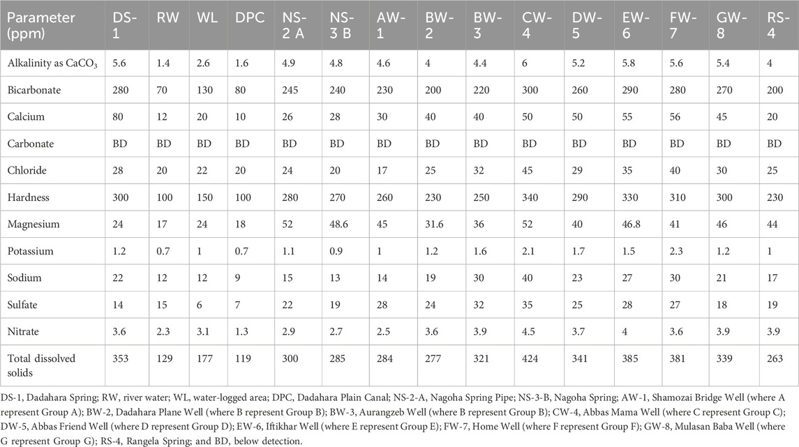
Table 1. Physicochemical characteristics of water samples collected from different locations in the Swat District.

3.3 Geochemistry of rock samples

The geochemical compatibility of different oxides was examined using X-ray fluorescence spectroscopic analysis. The different oxides and elements present in rock samples are presented in Table 2. The highest amount of silicon dioxide was obtained in all rock samples. The maximum SiO₂ was found in DRS-1 (61.193), followed by RRS-4 (49.144), NRS-3 (16.688), and DPRS-2 (12.184). DRS-1 samples contained aluminum oxide (20.62), calcium oxide (8.54), iron (III) oxide (4.93), potassium oxide (3.62), titanium oxide (0.79), strontium oxide (0.067), manganese oxide (0.057), vanadium pentoxide (0.045), chromium oxide (0.025), rubidium oxide (0.017), copper oxide (0.016), zinc oxide (0.015), iridium oxide (0.011), and yttrium oxide (0.003), and nickel oxide and sulfur oxide were not observed. The oxides of vanadium, zirconium, chromium, rubidium, zinc, iridium, yttrium, and sulfur were not found in DPRS-2. Moreover, rubidium oxide, yttrium oxide, nickel oxide, and sulfur oxide were not observed in RRS-4. Oxides of zirconium, iridium, yttrium, and nickel were not detected in NRS-3.

Table 2

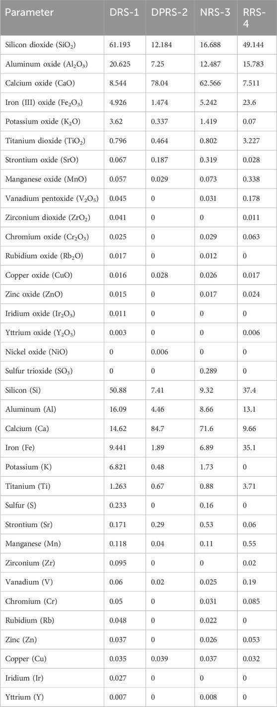
Table 2. a) Different oxides observed in rock samples from the Swat District. b) Different elements observed in rock samples from the Swat District.

3.4 Well cross-sections and their respective logs

This research investigates the relationship between the variations in depth of the water table in response to its variable distance from the Swat River in the representative wells within the study area. The study area is divided into seven distinct groups, ranging from Group A to Group G, each encompassing five representative wells (Figure 3). The primary objective is to understand how the water level in these wells varies as we move away from the river. The lithological composition of the wells includes gravel, soil, and bedrock, which serve as potential reservoirs/aquifers for groundwater accumulation.

3.5 Machine learning

3.5.1 Model performance analysis

3.5.1.1 Linear regression

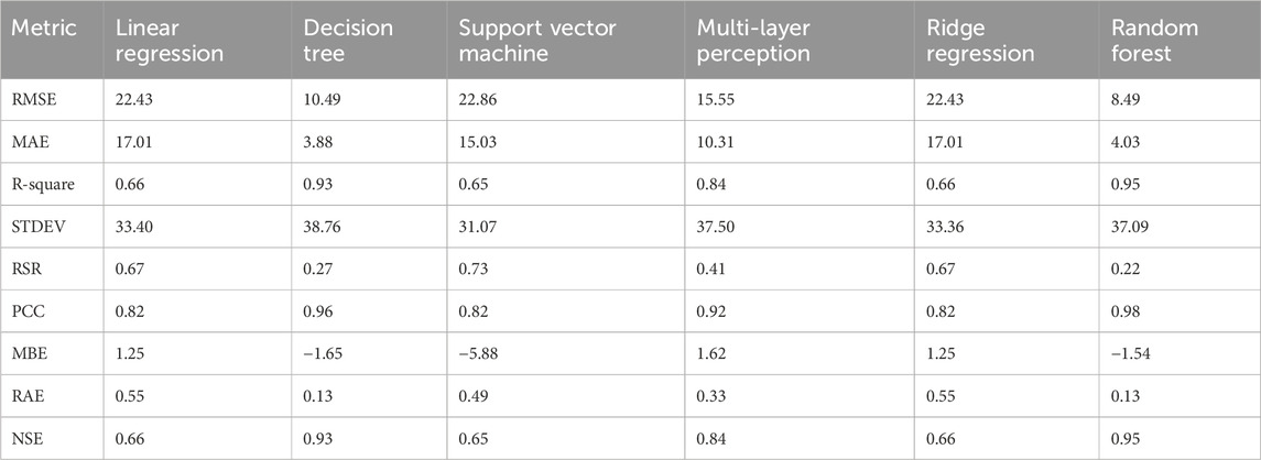
RMSE = 22.43, MAE = 17.01, and R² = 0.66.

Linear regression shows high root mean square error (RMSE) and mean absolute error (MAE), indicating higher prediction errors. R² value reveals a moderate correlation, but it is not highly significant.

3.5.1.2 Decision tree

RMSE = 10.49, MAE = 3.88, and R² = 0.93.

The decision tree model performs well with low values of RMSE and MAE, which indicate smaller prediction errors made by the model during training. An R² value of 0.93 indicates a very strongly correlation with the actual values.

3.5.1.3 Support vector machine

RMSE = 22.86, MAE = 15.03, and R² = 0.65.

Among the models, SVM has the highest RMSE, indicating poor performance; it also has a high MAE, while its R² value is low, thus suggesting that this model does not fit the data well.

3.5.1.4 Multi-layer perceptron

RMSE = 15.55, MAE = 10.31, and R² = 0.84.

Compared to other models, MLP performs moderately, maintaining RMSE and MAE values balanced for prediction purposes. The achieved R² value demonstrates a good fit though not as strong as that of the decision tree and random forest models.

3.5.1.5 Ridge regression

RMSE = 22.43, MAE = 17.01, R² = 0.66.

In terms of results, ridge regression is similar to linear regression, exhibiting relatively high prediction errors and a moderate correlation coefficient.

3.5.1.6 Random forest

RMSE = 8.49, MAE = 40.3, and R² = 95.

The smallest RMSE and MAE values indicate that random forest outperforms all other models by making the most precise predictions. An excellent fit, reflected by an R² value of 0.95, shows that this model accounts for 95% of the variance in the data.

In addition to predicting chemical concentration trends, the models were used to identify spatial zones with high groundwater potential based on their predictive scores, lithological context, and recharge proximity. Model performance was validated using RMSE, MAE, and R² values. Among all, random forest performed best (RMSE = 8.49 and R² = 0.95), followed by decision tree (R² = 0.93). Cross-validation techniques ensured robustness and minimized overfitting. Visual plots further confirmed model reliability. The machine learning-based classification enabled the demarcation of feasible GWPZs, aligning with the objective of well location optimization mentioned in the introduction.

All model configurations of each machine learning model showed that the PCC values ranged from 0.82 to 0.98. This range illustrates that there was a strong to very strong positive linear correlation between the observed and predicted values. The highest correlation (PCC = 0.98) demonstrates great model fit and is particularly important when trends need to be captured accurately. What stood out were the MBE values, which ranged from −5.88 to 1.62, illustrating that some models slightly overestimate, while others underestimate the values; however, the biases are generally acceptable. The MBE value of −5.88 for one model shows a tendency to underestimate, suggesting that the model may need further calibration.

The MBE values also mark the boundaries at which models can be considered robust. RAE values ranging from 0.13 to 0.55 indicate that the model predictions are reliable, with lower values indicating better performance in minimizing relative error compared to a naive benchmark model (i.e., mean predictor). The NSE values ranging from 0.65 to 0.95 corroborate the models’ reliability. An NSE value greater than 0.5 denotes superior model performance compared to the mean value extracted from the observed data. Values nearing 1 indicate high skill in prediction. It is clear that the model with NSE = 0.95 performs excellently as it captures both the variability and magnitude of the data.

3.5.1.7 Graphical representation

These images illustrate the comparison between predicted and actual values for each model. Decision tree and random forest models closely align with the actual data points, visually confirming their superior performance. In contrast, linear regression, ridge regression, and SVM show greater deviations from the actual values, implying poorer performance. The MLP model produces predictions that are very close to the ground truth though some fluctuations are present.

4 Interpretation of results: recharge source and groundwater potential mapping

This section interprets the analytical and model-based results presented in Section 3 (Results), with a focus on identifying groundwater recharge mechanisms and delineating GWPZs using machine learning predictions.

4.1 Geochemistry of water samples

4.1.1 Calcium carbonate

Interpretation of the analytical data reveals that the concentration of CaCO₃ is variable in the investigated water samples collected from different locations. Furthermore, the amount of calcium carbonate is very high in Dadahara Spring, Group C well (CW-4), and Rangela Spring, representing the association of these water samples with carbonate-bearing rocks (Figure 4A). The percolated water has passed through carbonate-bearing rocks, i.e., marble, which has enhanced the concentration of dissolved CaCO₃ ions in the analyzed samples. The dashed line indicates the increasing concentrations of CaCO₃ with increasing distance of the wells/location of collected water samples from the Swat River. Increasing distance from the main recharge source (i.e., Swat River) indicates that the percolation and infiltration of surface water (from streams and rainfall) through carbonate-bearing rocks cause chemical weathering/dissolution, resulting in higher CaCO₃ concentrations in water (Figure 4A).

Figure 4

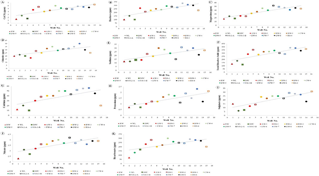
Figure 4. Graphs representing the concentration of (A) calcium carbonate, (B) hardness, (C) magnesium, (D) chloride, (E) sodium, and (F) total dissolved solids detected in the water samples against their respective wells and springs, representing an increase in the concentration of (A) calcium carbonate, (B) hardness, (C) magnesium, (D) chloride, (E) sodium, and (F) total dissolved solids. Graphs representing the concentration of (G) calcium, (H) potassium, (I) sulfate, (J) nitrate, and (K) bicarbonate detected in the water samples against their respective wells and springs, representing an increase in the concentration of (G) calcium, (H) potassium, (I) sulfate, (J) nitrate, and (K) bicarbonate in the water samples collected from representative wells.

4.1.2 Hardness

Geochemical data interpretation reveals that hardness is variable in the investigated water samples collected from different locations in the study area. Moreover, hardness is very high in Group E well (EW-6), Group F well (FW-7), and Group G well (GW-8), representing the association of these water samples with calcium- and magnesium-bearing rocks (Figure 4B). The percolated water has passed through these rocks and enhanced the concentration of dissolved calcium and magnesium ions in the analyzed samples. The dashed line indicates the rising trend of hardness with increasing distance of the wells/location of the collected water samples from the Swat River. Increasing distance from the main recharge source (i.e., Swat River) indicates that the percolation and infiltration of surface water (streams and rainfall) through these rocks cause chemical weathering/dissolution, leading to an increase in hardness in the water.

4.1.3 Magnesium

Interpretation of the geochemical data reveals that the concentration of magnesium is variable in the examined water samples collected from different locations. Additionally, the amount of magnesium is very high in Nagoha Spring, Nagoha Spring Pipe, and Group E well (EW-6), representing the association of these water samples with magnesium-bearing rocks (Figure 4C). The percolated water has passed through the magnesium-bearing rocks, i.e., dolomitic marble [Ca(MgCO₃)₂] and serpentine-bearing rocks, which has enhanced the concentration of dissolved Mg ions in the examined samples. The dashed line indicates the increasing concentrations of Mg with increasing distance of the wells/location of collected water samples from the Swat River. Increasing distance from the main recharge source (i.e., the Swat River) indicates that the percolation and infiltration of surface water (streams and rainfall) through the magnesium-bearing rocks cause chemical weathering/dissolution, leading to an increase in the magnesium concentration in the water.

4.1.4 Chloride

The interpretation of analytical data indicates variations in the concentration of chloride among the investigated water samples collected from different locations. The analysis of chloride (Cl^1-) concentration across the examined water locations reveals a consistent and notable increase in their levels with increasing distance (Figure 4D). This trend indicates that various geological and hydrological factors contribute to the observed chloride variations, particularly in areas such as Group C (CW-4) and Group F (FW-7) where the concentrations are prominently elevated. The increasing concentrations of chloride are likely influenced by factors such as the dissolution of chloride-bearing minerals or anthropogenic inputs. The proximity of CW-4 and FW-7 to potential sources of chloride, such as chloride-bearing rocks, urban areas, or agricultural activities could contribute to the higher chloride levels observed in these locations. Additionally, the pattern of increasing chloride concentrations with increasing distance from the Swat River suggests that the percolation of surface water through the rocks plays a role in transporting chloride ions into the subsurface water sources, which results in an increase in the concentration of chloride in the water.

4.1.5 Sodium

Interpretation of the analytical data reveals that the concentration of sodium is variable in the examined water samples collected from different locations. Furthermore, the amount of sodium is very high in Group B well (BW-3), Group F well FW-7, and Nagoha Spring Pipe, representing the association of these water samples with sodium-bearing rocks (Figure 4E). The percolated water has passed through the sodium-bearing rocks, which has enhanced the concentration of dissolved Na ions in the studied samples. The dashed line indicates the ascending concentrations of sodium with increasing distance of the wells/location of collected water samples from the Swat River. Increasing distance from the main recharge source (i.e., Swat River) indicates that the percolation and infiltration of surface water (streams and rainfall) through sodium-bearing rocks cause chemical weathering/dissolution, leading to an increase in the sodium concentration in the water.

4.1.6 Total dissolved solid

Total dissolved solids (TDS) are a measure of the combined content of all inorganic and organic substances dissolved in water. It includes minerals, salts, metals, cations, anions, and sometimes even small amounts of organic matter.

Interpretation of the analytical data reveals that the concentration of TDS is variable in the inspected water samples collected from different locations in the studied area. Furthermore, the amount of TDS is very high in Dadahara Spring, Group E well (EW-6), and Group F well (FW-7). A cross plot of TDS vs. analyzed samples indicates that the concentrations of TDS increase with increasing distance of the wells/location of collected water samples from the Swat River (Figure 4F). Increasing distance from the main recharge source (i.e., Swat River) indicates that the percolation and infiltration of surface water (streams and rainfall) pass through rocks susceptible to dissolution or chemical weathering, leading to an increase in TDS concentrations in the water.

4.1.7 Calcium

Cross plot of Ca versus their corresponding sample locations illustrates that the concentration of calcium varies randomly in the examined water samples collected from the studied area. In particular areas such as Group C well (CW-4), Group D well (DW-5), Nagoha Spring, Group E well (EW-6), and Group F well (FW-7) stand out with notably high calcium concentrations, implying a close connection to calcium-bearing rocks (Figure 4G). The concentration of calcium (Ca²⁺) across the analyzed water sample reveals a consistent trend of increasing levels with ascending distance from the Swat River. The observed pattern indicates that the percolation of water through calcium-rich rocks, such as marble, or other calcium-bearing rocks like calcic-rich schists, serves as a source of calcium content in the water samples. The increasing concentration of Ca in different water samples is illustrated by a dashed line in the acquired cross plot, which shows that water samples collected from mountainous area possess higher amount of calcium. This increase in the concentration of Ca suggests that the percolated water has interacted with surface/sub-surface rocks, dissolved Ca ions from rocks, and then added them to the groundwater.

4.1.8 Potassium

Analytical data interpretation reveals that the concentration of potassium is variable in the investigated water samples collected from different locations. Again, the amount of potassium is very high in Nagoha Spring Pipe, Group F well (FW-7), and Rangela Spring, representing the association of these water samples with potassium-bearing rocks (Figure 4H). The percolated water has passed through the potassium-bearing rocks, which has enhanced the concentration of dissolved potassium ions in the analyzed samples. The dashed line in the cross plots indicates a linear trend, representing the increasing concentrations of potassium with increasing distance of the wells/location of collected water samples from the Swat River (Figure 4H). Increasing distance from the main recharge source (i.e., Swat River) indicates that the percolation and infiltration of surface water (streams and rainfall) through the potassium-bearing rocks cause chemical weathering/dissolution, leading to an increase in the potassium concentration in the water.

4.1.9 Sulfate

Geochemical data interpretation of water samples reveals that the concentration of sulfate is variable in the examined samples collected from different locations. It has been observed that the concentration of sulfate is very high in samples collected from Nagoha Spring Pipe, Group E well (EW-6), and Rangela Spring, representing the association of these water samples with sulfate-bearing rocks (Figure 4I). The percolated water has passed through the sulfate-bearing rocks, which has enhanced the concentration of dissolved sulfate ions in the examined samples. The dashed line in the cross plot of sulfate versus the sample’s location indicates the increasing concentrations of sulfate with increasing distance of the wells/location of collected water samples from the Swat River (Figure 4I). Increasing distance from the main recharge source (i.e., Swat River) indicates that the percolation and infiltration of surface water (streams and rainfall) through the sulfate-bearing rocks cause chemical weathering/dissolution, leading to an increase in the sulfate concentration in the water.

4.1.10 Nitrate

Interpretation of the analytical data reveals that the concentration of nitrate is variable in the investigated water samples collected from different locations. It has been observed that the concentration of nitrate is very high in Group C well (CW-4), Nagoha Spring, and Group E well (EW-6), representing the association of these water samples with nitrate-bearing rocks/soil (Figure 4J). It demonstrates that the percolated and infiltrated rainwater has passed through the nitrate-bearing rocks/soil zones, which has enhanced the concentration of dissolved nitrate ions in the examined samples. A cross plot of the acquired nitrate concentration vs. their sampling location illustrates the ascending concentrations of nitrate with increasing distance of the wells/location of collected water samples from the Swat River. Increasing distance from the main recharge source (i.e., Swat River) indicates that the percolation and infiltration of surface water (streams and rainfall) through these rocks/soil horizons cause chemical weathering/dissolution, leading to an increase in nitrate ions in groundwater.

4.1.11 Bicarbonate

Interpretation of the analytical data demonstrates variability in bicarbonate concentration observed among the investigated water samples collected from various locations of the investigated area. The interpreted data underscores a consistent trend of increasing bicarbonate (HCO^3-) concentrations across the water samples collected from different locations. Notably, the concentration of bicarbonate is found to progressively increase (Figure 4K). This pattern is particularly pronounced in areas such as Dadahara Spring (DS-1), Group C well (CW-4), and Group E well (EW-6), where the presence of bicarbonate-rich minerals or rock is evident, like marble, which contains calcium carbonate (CaCO₃) minerals that can release bicarbonate ions (HCO^3-) into the water as the rock dissolves over time. The observed trend suggests that subsurface water sources contribute to the elevated bicarbonate levels. As water percolates through the surrounding rocks, it interacts with carbonate minerals, dissolving and carrying bicarbonate ions into the groundwater reservoirs. The dashed line shows an increasing concentration of bicarbonate with increasing distance of the wells/location of collected water samples from the Swat River. The progressive increase in distance from the Swat River suggests that the percolation and infiltration of surface water (streams and rainfall) through rocks containing carbonates result in chemical weathering and dissolution. This process leads to an increase in bicarbonate levels in the water.

4.2 Geochemistry of rock samples

Geochemical studies using XRF on rock samples are generally conducted to determine their elemental composition. XRF is an analytical technique that provides information on the presence and concentration of various elements within a bulk rock sample. By subjecting the rock sample to XRF analysis, the composition, and the concentrations of elements can be identified, such as major elements (e.g., silicon, aluminum, iron, calcium, magnesium, sodium, and potassium) and trace elements (e.g., zinc, copper, nickel, and chromium) observed in this study.

Cross plots between the above-mentioned elements were established to understand the geochemical compatibility of different oxides and their corresponding relative trends.

Upon analyzing the scatter plots, it was observed that some rock samples exhibited a positive correlation between different oxides, suggesting a potential chemical compatibility between these elements. These samples formed a trend line that inclined upward or downward, indicating an increase or a decrease in the concentration of oxides. There were also rock samples that displayed a negative or no clear relationship between the observed oxides. These samples appeared as scattered points across the plot, indicating a lack of significant association or compatibility with respect to the plotted oxides.

Groups of rock samples with similar oxide values were also observed, indicating the presence of distinct mineral assemblages in the investigated rock samples collected from the study area. These clusters provided valuable insights into the geochemical variations and rock composition in the analyzed samples. The plotted data allowed for a visual exploration of the geochemical compatibility between different oxides. The scatter plots provided a comprehensive overview of the relationship between these elements, aiding in the interpretation and understanding of the geochemical characteristics of the studied rock samples.

4.2.1 Geochemical compatibility of calcium and iron oxides

Variable calcium oxide values, i.e., 8.54%, 78.06%, 62.56%, and 7.51%, and iron oxide values (4.93%, 1.47%, 5.24%, and 23.6%) were detected in the investigated rock samples. In order to understand the relative trend and the geochemical compatibility of the elemental composition in the analyzed rock samples, a cross plot between CaO and Fe₂O₃ has been established (Figure 5A). This shows an inverse relationship between CaO and Fe₂O₃ contents, respectively (Figure 5A). The given cross plot demonstrates that the quantity of CaO increases as the concentration of Fe₂O₃ decreases. As evident, DPRS-2 and NRS-3 rock samples possess the highest CaO concentration (78.06% and 62.56%, respectively) and the lowest Fe₂O₃ concentration (1.47% and 5.24%, respectively). On the other hand, rock samples collected from Dadahara Spring (DRS-1) and Rangela Spring (RRS-4) exhibit relatively low CaO content (8.54% and 7.51%) and significantly higher Fe₂O₃ concentration (4.93% and 23.6%). A cross plot of CaO versus Fe₂O₃ shows an inverse trend, demonstrating that the concentration of Fe₂O₃ decreases with the increasing concentration of CaO. Furthermore, it indicates that CaO and Fe₂O₃ are not geochemically compatible. Samples collected from springs located in carbonate-bearing rocks indicate higher concentrations of CaO (e.g., Dadahara Plain and Nagoha Spring) and lower concentrations of Fe₂O₃.

Figure 5

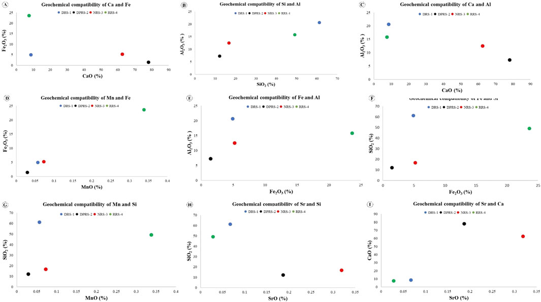
Figure 5. Cross plot representing the mineralogical composition of the analyzed rock samples. (A) CaO vs. Fe₂O₃, (B) SiO₂ vs. Al₂O_3, (C) CaO vs. Al₂O_3, and (D) MnO vs. Fe₂O₃, representing the geochemical variability of (A) calcium carbonate and iron oxide, (B) silica and aluminum oxides, (C) calcium and aluminum oxides, and (D) manganese and iron oxides. (E) Fe₂O₃ vs. Al₂O₃, (F) Fe₂O₃ vs. SiO_2, (G) MnO vs. SiO₂, (H) SrO vs. SiO₂, and (I) SrO vs. CaO, representing the geochemical variability of (E) iron and aluminum oxides, (F) iron and silica oxides, (G) manganese and silicon oxides, (H) strontium and silica oxides, and (I) strontium and calcium oxides in the investigated rock sample.

4.2.2 Geochemical compatibility of silica and aluminum oxides

Detected SiO₂ values (i.e., 61.19%, 12.18%, 16.69%, and 49.14%) and Al₂O₃ values (i.e., 20.62%, 7.25%, 12.49%, and 15.78%) in the representative rock samples exhibit measurable variability. In order to better understand the relative trend of elemental composition in different rock samples, a cross plot of SiO₂ versus Al₂O₃ has been established (Figure 5B). The given figure illustrates a direct relationship between the concentrations of silica oxide and aluminum oxide. The linear trend indicates that the concentration of Al₂O₃ gradually increases with the increasing concentration of SiO₂. The interpreted data presented in the figure show that as the amount of Al₂O₃ increases, the amount of SiO₂ also increases (Figure 5B). Interpretation of geochemical data demonstrates that the rock samples collected from Dadahara Plain and Nagoha Spring correspond to silica-deficient rocks, i.e., most probably, marble. Similarly, the concentration of SiO₂ is much higher in the rock samples representing Dadahara and Rangela springs, resembling the chemical composition of acidic igneous/metamorphosed pelitic rocks.

4.2.3 Geochemical compatibility of calcium and aluminum oxides

Variable concentrations of CaO (8.54%, 78.06%, 62.56%, and 7.51%) and Al₂O₃ (20.62%, 7.25%, 12.48%, and 15.78%) were detected during geochemical investigations. To understand the geochemical relationship between CaO and Al₂O₃ distribution in the examined rock samples, a cross plot of CaO versus Al₂O₃ has been established (Figure 5C). The interpreted data shows an inverse relationship between CaO and Al₂O₃ contents (Figure 5C). The figure shows an extremely contrary association between CaO and Al₂O₃ contents among these rock samples. Dadahara and Rangela spring rock samples exhibit higher concentrations of Al₂O₃ and lower levels of CaO. On the other hand, the rock samples collected from the vicinity of Dadahara Plain and Nagoha Spring display higher percentages of CaO and lower amounts of Al₂O₃. This observation indicates a distinct contrast in the composition of these rocks, possibly reflecting different mineralogical compositions or geological origins. The elevated concentration of CaO represents calcium-rich rock, i.e., marble, while the higher amount of Al₂O₃ demonstrates metamorphosed pelitic rocks.

4.2.4 Geochemical compatibility of manganese and iron oxides

Minor oxides, i.e., MnO values detected in the investigated rock samples are 0.05%, 0.02%, 0.07%, and 0.33%, whereas the acquired Fe₂O₃ values in these samples are 4.92%, 1.47%, 5.24%, and 23.6%. In order to understand a probable relationship between MnO and Fe₂O₃ distribution in the representative rock samples, a cross plot of MnO vs. Fe₂O₃ has been established (Figure 5D). The given cross plot exhibits a direct relationship and linear trend between MnO and Fe₂O₃, respectively (Figure 5D). The cross plot shows variations in the manganese and iron content among different rock samples. The concentration of MnO increases with the increasing concentration of Fe₂O₃ in the investigated rock samples. A high percentage of Fe₂O₃ and MnO in the RRS-4 sample illustrates its derivation from a ferromagnesian mineral-rich metamorphosed rock, while the lower concentration of Fe₂O₃ and MnO in DRS-1, DPRS-2, and NRS-3 indicate a lack of ferromagnesian minerals in the investigated rock samples. Lower concentrations of Fe and Mn are mostly associated with acidic igneous rocks or calcareous rocks.

4.2.5 Geochemical compatibility of iron and aluminum oxides

Extremely variable concentrations of Fe₂O₃ (4.92%, 1.47%, 5.24%, and 23.6%) and Al₂O₃ (20.62%, 7.25%, 12.48%, and 15.78%) were detected during the geochemical investigation of the representative rock samples. In order to understand the probable geochemical relationship between Fe₂O₃ and Al₂O₃ in various rock samples, a cross plot between Fe₂O₃ and Al₂O₃ has been established, which indicates a direct relationship between the concentrations of Fe₂O₃ and Al₂O₃ except the DPRS-2 rock sample. DPRS-2 samples exhibit an inverse relationship to the overall trend between Fe₂O₃ and Al₂O₃. Interpretation of the detected data demonstrates that the amount of Fe₂O₃ increases with the increasing concentrations of Al₂O₃ (Figure 5E). To conclude, a direct geochemical relationship has been found between Fe₂O₃ and Al₂O₃ in the DRS-1, NRS-3, and RRS-4 rock samples. High percentages of Al₂O₃ in DPRS-2 illustrate metamorphosed pelitic rock, while the higher concentration of Fe₂O₃ in RRS-4 exhibits the ferromagnesian character of the investigated rock sample.

4.2.6 Geochemical compatibility of iron and silica oxides

Fe₂O₃ values determined in representative rock samples are 4.93%, 1.47%, 5.24%, and 23.61%, whereas SiO₂ values are 61.19%, 12.18%, 16.69%, and 49.14%. In order to understand the geochemical relationship between Fe₂O₃ and SiO₂ distribution in the investigated rock samples, a cross plot between Fe₂O₃ and SiO₂ has been established (Figure 5F). The cross plot of Fe₂O₃ vs. SiO₂ illustrates a direct relationship between the concentrations of iron oxide and silicon oxide. There is a linear trend (the amount of silica increases with increasing concentration of silica), which represents a direct relation between Fe₂O₃ and SiO₂ in the DPRS-2, NRS-3, and RRS-4 rock samples. The percentages of Fe₂O₃ and SiO₂ are much higher in RRS-4 and lower in DPRS-2, exhibiting two different lithological units, i.e., SiO₂-rich and SiO₂-deficient, respectively. DRS-1 illustrates contrasting geochemical behavior, e.g., a lower concentration of Fe₂O₃ and a very high amount of SiO₂, indicating a metamorphosed intermediate/acidic igneous rock.

4.2.7 Geochemical compatibility of manganese and silicon oxides

Major and minor oxides with variable concentrations were detected in the investigated rock samples, which include SiO₂ (61.19%, 12.18%, 16.68%, and 49.14%) and MnO (0.05%, 0.02%, 0.07%, and 0.33%), respectively. These major and minor oxides were plotted in order to determine geochemical compatibility between SiO₂ and MnO in the investigated rock samples. The acquired cross plot demonstrates a direct relationship between the increasing concentrations of manganese oxide and the ascending amount of silicon oxide. DPRS-2 and NRS-3 exhibit lower concentration of SiO₂, which is an indication of silica-deficient rock, i.e., marble. Similarly, the concentration of SiO₂ is high in the DRS-1 and RRS-4 rock samples, which is indicative of silica-rich metamorphosed rocks. The data presented in the figure show that as the amount of manganese increases, the amount of silica also increases (Figure 5G). Except for DRS-1, there is a direct relationship between SiO₂ and MnO in the investigated rock samples, which illustrates that these minerals are geochemically compatible with each other.

4.2.8 Geochemical compatibility of strontium and silicon oxides

Variable concentrations of SrO determined in the examined rock samples are 0.06%, 0.18%, 0.31%, and 0.02%, whereas similar variations in the SiO₂ contents were also observed, i.e., 61.19%, 12.18%, 16.68%, and 49.14%, respectively. The detected major (SiO₂) and minor (SrO) oxides were then used to determine their geochemical compatibility in the inspected rock samples. In order to understand the relative trend of the abovementioned elemental composition in different rock samples, a cross plot between SrO and SiO₂ has been established (Figure 5H). The cross plot of these major and minor oxides indicates an inverse relationship between the concentrations of strontium oxide and silicon oxide. The concentration of SiO₂ is high in the DRS-1 and RRS-4 samples, while the amount of SrO is very low in these samples. Similarly, the percentage of SiO₂ oxide is very low in DPRS-2 and NRS-3, whereas the concentration of SrO is high in these samples. Based on the abovementioned observations in the given cross plot, SiO₂ is not geochemically compatible with SrO (Figure 5H). It is clearly shown in the graph that the amount of SrO decreases with the increasing concentration of SiO₂ and vice versa. Furthermore, it demonstrates that calcium-rich rock, i.e., marble, possesses a high amount of Sr, while silica-rich rocks are deficient in Sr.

4.2.9 Geochemical compatibility of strontium and calcium oxides

Major and minor oxides detected in the investigated rock samples collected from the study area include variable concentrations of SrO (0.06%, 0.18%, 0.31%, and 0.02%) and CaO (8.54%, 78.06%, 62.56%, and 7.51%), respectively. Normally, we cannot classify rock types on the basis of trace elements/oxides, but it can be used for the determination of geochemical compatibility. Minor oxide (SrO) was plotted against major oxide (CaO), and a relatively direct relationship was observed between the concentrations of strontium oxide and calcium oxide. The cross plot exhibits that the concentrations of SrO and CaO are lower in DRS-1 and RRS-4, while the amounts of SrO and CaO are high in the DPRS-2 and NRS-3 samples. There is a direct relationship between these oxides, i.e., the percentage of SrO increases with increasing CaO contents, which illustrates a linear trend. Based on the abovementioned values of the examined rock samples, SrO is geochemically compatible with CaO (Figure 5I). Furthermore, the concentrations of CaO and SrO are high in DPRS-2 and NRS-3, representing calcareous-rich rock, i.e., marble.

5 Discussion

Data collected during detailed field activity, i.e., distance from the Swat River, water depth, depth of the well, and lithological variation in the well, were plotted in cross-sections, and a direct relationship was observed between water depth and distance from the Swat River. Increasing water depth in wells represents its increasing distance from the main recharge source, i.e., Swat River.

Atomic absorption spectroscopic studies of the collected water samples from representative wells of each group, nearby springs, water-logged areas, and canals demonstrate that the probable recharge source for groundwater in the lower Swat area is the Swat River, as well as its contributory channels and rainwater. Acceptable similarities were observed in the geochemical composition of the rock samples, spring water samples, and representative wells in their immediate neighborhood.

Similarly, X-ray fluorescence analysis of the spring’s host rocks was compared with the dissolved mineral constituents of the analyzed water samples, and it was noted that the concentration of rock-forming minerals increases in water with increasing distance from the Swat River. This increase in dissolved minerals illustrates the interaction of groundwater with the bedrock during its migration from the source to the reservoir. Analytical data interpretation reveals that the recharge source for groundwater in the floodplain regime is the Swat River, while infiltration and percolation of rainwater act as probable recharge sources in the mountainous and elevated areas.

Overall, the data from all seven groups consistently demonstrate the impact of distance from the Swat River on the fluctuation of groundwater level in the floodplain area of the Swat River. The progressive decrease in the water level as we move away from the river supports the understanding that proximity to the river is a crucial factor affecting groundwater resources in the study area. Two main aquifers were encountered in this study, i.e., gravel deposited by the Swat River in its floodplain and fractured bedrock. The primary recharge sources for these aquifers include the main trunk and contributory channels of the Swat River, irrigation channels derived from the Swat River, and surface precipitation. More than 80% of the producing wells have been drilled in the gravel layer, while bedrock contributes only 20% as an aquifer. The study area is covered with high-grade metamorphic rocks. Normally, metamorphic rocks do not possess porosity and permeability for the accumulation of groundwater. In this case, intense fractures and inclined geometries of the bedrock provide the best possible pathways for the primary migration of rainwater into the main aquifer.

Group G comprises several representative wells located within a range of 2,501–3,000 m from the Swat River. These wells have water table/level depths ranging from 80 feet to 220 feet. The obtained graph from field data presents the relationship between distance from the Swat River and water table/level depth for Group G (Figure 6). The upward-sloping predicted line indicates that water table/level depths tend to increase with an increase in the distance from the river. The linear regression model’s predicted line serves as a valuable tool for predicting water table/level depths in wells at different distances from the Swat River.

Figure 6

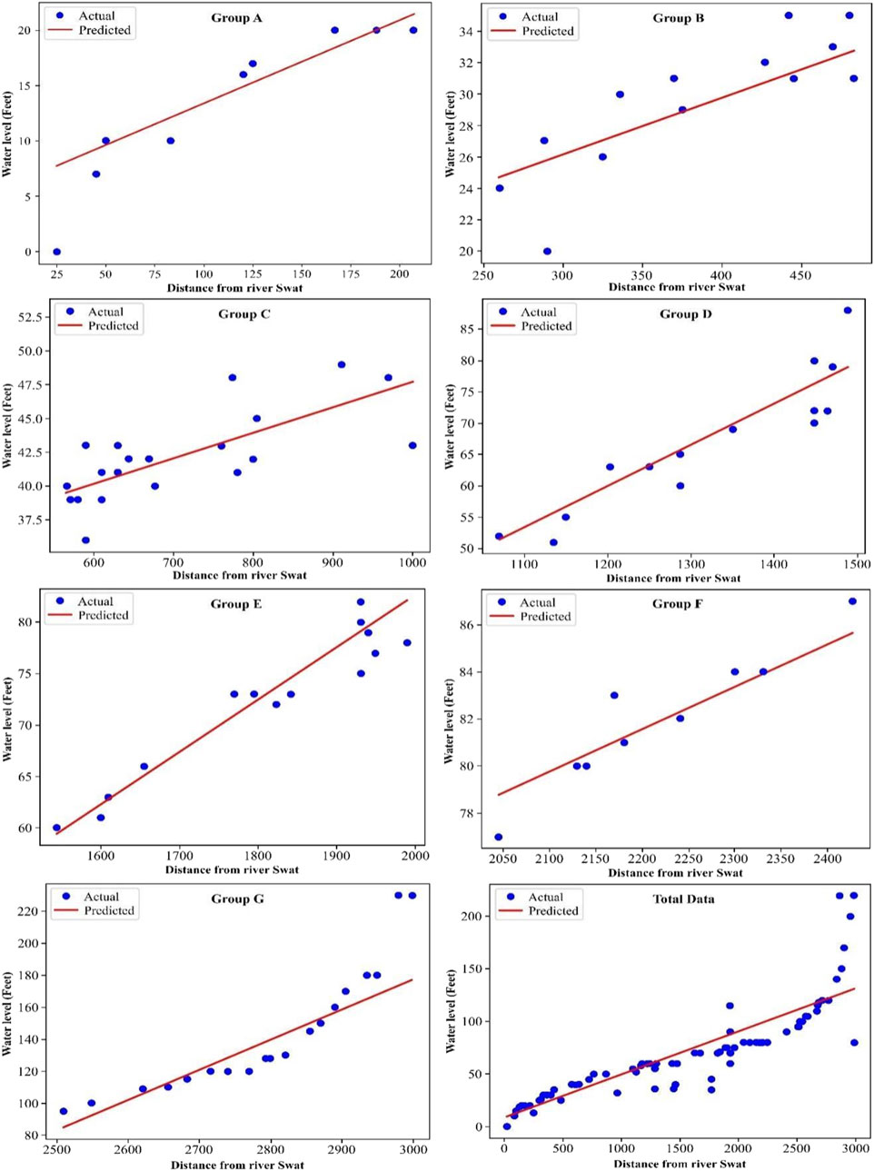
Figure 6. Cross plot of the observed water level depth in wells of Group G vs. its distance from the Swat River, representing actual data and a predicted line for water level depth with increasing distance from the Swat River.

The cross plot compares the observed depth of the water table/level in wells of Group G with their respective distances from the Swat River. The plot includes both actually acquired data and a predicted line, which represents a linear trend of water table/level depth with the increasing distance from the Swat River (Figure 6). The predicted line is obtained from a machine learning program (linear regression model), which allows us to predict the actual depth of the water table/level in the potential zone of floodplain region of the Swat River at variable distances from the river (Figure 7).

Figure 7

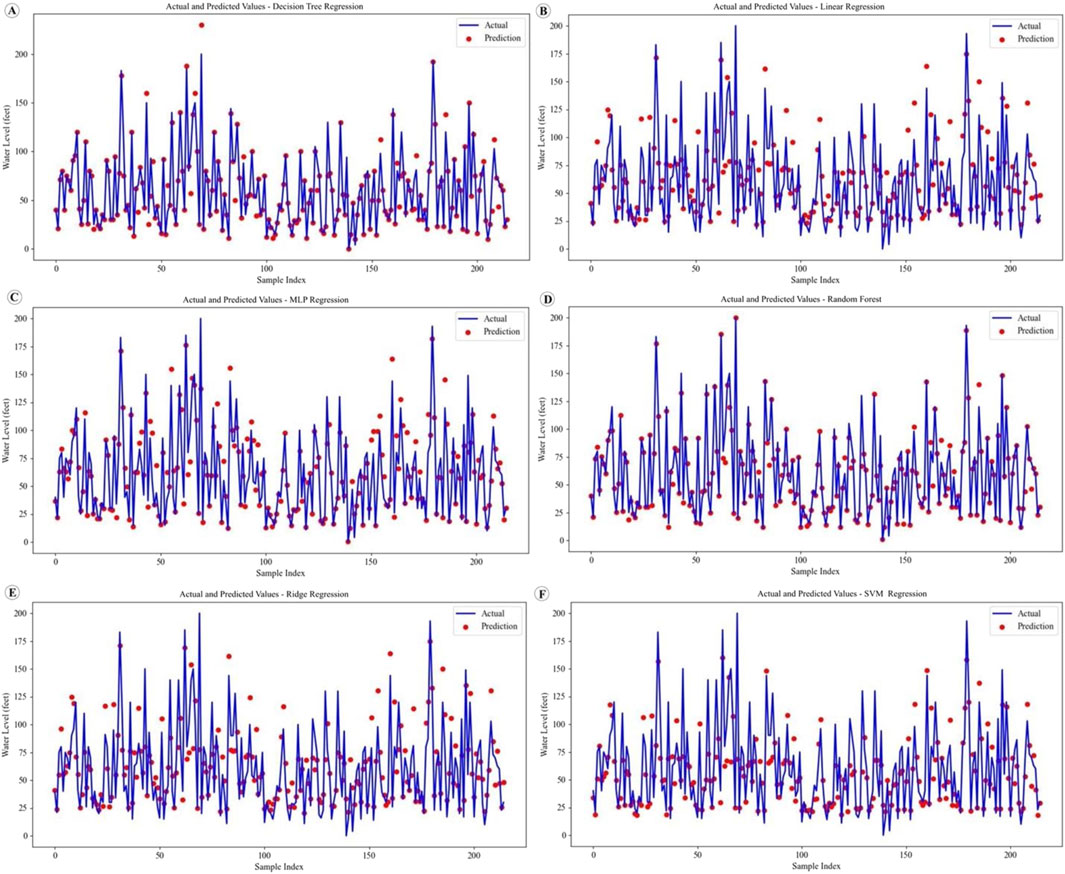
Figure 7. Cross plot exhibiting the observed water depth in the studied wells vs. its distance from the Swat River, representing actual data and predicted water depth with increasing distance from the Swat River using the (A) decision tree regression model, (B) linear regression model, (C) MLP regression model, (D) random forest model, (E) ridge regression model, and (F) SVM regression model.

Water table/level depths were plotted against their respective distances from the Swat River, and a general trend of increasing water table/level depth with increasing distance from the river in the floodplain regime was observed. The acquired data were then plotted and processed using the linear regression model of the machine learning program. We obtained a predicted line for the drilling of wells in suitable locations with the defined depth of the water table/level and its corresponding distance from the river in the floodplain area. The use of linear regression is very helpful in the accurate demarcation of potential groundwater zones in the investigated area. It has been concluded from this study that the obtained predicted line demonstrates a linear trend, indicating that as the distance from the river increases, the water table/level depth in the wells also increases (Figure 7).

The observed recharge mechanisms (river infiltration in floodplain zones and rainwater percolation in elevated zones) are consistent with findings by Xu and Beekman (2003) in southern Africa and Panda et al. (2020) in India. Similarly, our high model accuracy (R² = 0.95 for RF) parallels recent success in hybrid ML applications in groundwater prediction (Naghibi et al., 2017b). The results validate the reliability of coupling geochemical data with AI models for spatial groundwater forecasting, as also reported by Rahmati et al. (2016).

However, unlike prior studies that rely solely on remote sensing or modeling, our field-based, chemically validated approach enhances local relevance and reduces uncertainty. This multi-source validation provides a significant methodological advancement.

5.1 Future perspectives

The findings of this study lay the foundation for future groundwater exploration in data-scarce mountainous regions. Integration of remote sensing and real-time hydrological data with AI-driven models could significantly enhance prediction accuracy. Moreover, the methodology developed in this study can be adapted for similar terrains in other parts of Pakistan and globally, aiding in the sustainable management of water resources under changing climatic conditions.

6 Conclusion

The severe exploitation of groundwater resources is compromising not only the quality but also the quantity of groundwater. In this study, acceptable similarities were observed in the geochemical composition of the rock samples, spring water samples, and representative wells in their immediate neighborhood. Moreover, the concentration of rock-forming minerals increases in water with increasing distance from the Swat River. This increase in dissolved minerals illustrates the interaction of groundwater with the bedrock during its migration from the source to the reservoir. Analytical data interpretation reveals that the recharge source for groundwater in the floodplain regime is the Swat River, while infiltration and percolation of rainwater act as probable recharge sources in the mountainous and elevated areas. The linear regression was observed between the water table and the distance from the Swat River, demonstrating that water depth in wells increases with increasing distance from the main recharge source. Different parameters (analytical data and field data) were plotted in Python and used to demarcate the predicted zones of potential groundwater in model wells using linear regression algorithms from machine learning techniques. The multi-model ML approach allowed for the cross-verification of predictions, while the use of geochemical compatibility analysis ensured field-based reliability. This combined methodology enhances the scientific validity and practical utility of the results, setting it apart from conventional single-model approaches.

Data availability statement

The original contributions presented in the study are included in the article/supplementary material; further inquiries can be directed to the corresponding authors.

Author contributions

IA: Writing – original draft, Resources, Supervision, Conceptualization. IU: Methodology, Writing – original draft, Investigation. MA: Writing – original draft, Visualization, Software. IG: Writing – review and editing. MK: Writing – review and editing, Validation. KK: Writing – review and editing, Methodology. UU: Investigation, Writing – review and editing. MR: Data curation, Writing – review and editing. MM: Writing – review and editing, Funding acquisition.

Funding

The author(s) declare that financial support was received for the research and/or publication of this article. This work has been funded by the Ongoing Research Funding program (ORF-2025-89), King Saud University, Riyadh, Saudi Arabia.

Conflict of interest

The authors declare that the research was conducted in the absence of any commercial or financial relationships that could be construed as a potential conflict of interest.

Generative AI statement

The author(s) declare that no Generative AI was used in the creation of this manuscript.

Publisher’s note

All claims expressed in this article are solely those of the authors and do not necessarily represent those of their affiliated organizations, or those of the publisher, the editors and the reviewers. Any product that may be evaluated in this article, or claim that may be made by its manufacturer, is not guaranteed or endorsed by the publisher.

References

Abdullahi, M. G., and Garba, I. (2015). Effect of rainfall on groundwater level fluctuation in Terengganu, Malaysia. J. Geophys. and Remote Sens. 4 (2), 142–146. doi:10.4172/2469-4134.1000142

CrossRef Full Text | Google Scholar

Ajith, M. P., and James, M. K. (2016). Impact of chamravattam regulator cum bridge on bharathapuzha river and adjacent areas. Indian J. Econ. Dev. 4 (1), 2320–9828.

Google Scholar

Akhtar, N., Syakir Ishak, M. I., Bhawani, S. A., and Umar, K. (2021). Various natural and anthropogenic factors responsible for water quality degradation: a review. Water 13, 2660. doi:10.3390/w13192660

CrossRef Full Text | Google Scholar

APHA (2017). Standard methods for the examination of water and wastewater. 23rd Edition. Washington, DC: American Public Health Association, American Water Works Association, Water Environment Federation.

Google Scholar

Arabameri, A., Rezaei, K., Cerda, A., Lombardo, L., and Rodrigo-Comino, J. (2019). GIS-Based ground water potential mapping in shahroud plain, Iran. A comparison among statistical (bivariate and multivariate), data mining and MCDM approaches. Sci. Total Environ. 658, 160–177. doi:10.1016/j.scitotenv.2018.12.115

PubMed Abstract | CrossRef Full Text | Google Scholar

Baart, F., de Boer, G., Pronk, M., van Koningsveld, M., and Muis, S. (2024). A semantic notation for comparing global high-resolution coastal flooding studies. Front. Earth Sci. 12, 1465040. doi:10.3389/feart.2024.1465040

CrossRef Full Text | Google Scholar

Bishop, C. M. (2006). Pattern recognition and machine learning. New York, NY: Springer.

Google Scholar

Boerner, A., and Weaver, C. (2012). Nebraska recharge estimation from chloride mass balance.

Google Scholar

Breiman, L. (2001). Random forests. Mach. Learn. 45, 5–32. doi:10.1023/a:1010933404324

CrossRef Full Text | Google Scholar

Carrard, N., Foster, T., and Willetts, J. (2019). Groundwater as a source of drinking water in southeast Asia and the Pacific: a multi-country review of current reliance and resource concerns. Water 11, 1605. doi:10.3390/w11081605

CrossRef Full Text | Google Scholar

Chen, W., Li, H., Hou, E., Wang, S., Wang, G., Panahi, M., et al. (2018). GIS-Based groundwater potential analysis using novel ensemble weights-of-evidence with logistic regression and functional tree models. Sci. Total Environ. 634, 853–867. doi:10.1016/j.scitotenv.2018.04.055

PubMed Abstract | CrossRef Full Text | Google Scholar

Crosbie, R. S., Binning, P., and Kalma, J. D. (2005). A time series approach to inferring groundwater recharge using the water table fluctuation method. Water Resour. Res. 41 (1). doi:10.1029/2004wr003077

CrossRef Full Text | Google Scholar

Das, B., and Pal, S. C. (2019). Combination of GIS and fuzzy-AHP for delineating groundwater recharge potential zones in the critical Goghat-II block of West Bengal, India. HydroResearch 2, 21–30. doi:10.1016/j.hydres.2019.10.001

CrossRef Full Text | Google Scholar

Domingos, P. (2012). A few useful things to know about machine learning. Commun. ACM 55 (10), 78–87. doi:10.1145/2347736.2347755

CrossRef Full Text | Google Scholar

Faheem, H., Khattak, Z., Islam, F., Ali, R., Khan, R., Khan, I., et al. (2023). Groundwater potential zone mapping using geographic information systems and multi-influencing factors: a case study of the kohat district, Khyber Pakhtunkhwa. Front. Earth Sci. 11, 1097484. doi:10.3389/feart.2023.1097484

CrossRef Full Text | Google Scholar

Golkarian, A., Naghibi, S. A., Kalantar, B., and Pradhan, B. (2018). Groundwater potential mapping using C5. 0, random forest, and multivariate adaptive regression spline models in GIS. Environ Ment. Monit. Assess. 190 (3), 149–16. doi:10.1007/s10661-018-6507-8

PubMed Abstract | CrossRef Full Text | Google Scholar

Goodfellow, I., Bengio, Y., and Courville, A. (2016). Deep learning. Cambridge, MA: MIT Press.

Google Scholar

Guru, B., Seshan, K., and Bera, S. (2017). Frequency ratio model for groundwater potential mapping and its sustainable management in cold desert, India. J. King Saud University-Science 29 (3), 333–347. doi:10.1016/j.jksus.2016.08.003

CrossRef Full Text | Google Scholar

Hastie, T., Tibshirani, R., Friedman, J., Hastie, T., Tibshirani, R., and Friedman, J. (2009). “Linear methods for regression,” in The elements of statistical learning: data mining, inference, and prediction, 43–99.

Google Scholar

Healy, R. W. (2010). Estimating groundwater recharge. United States: Cambridge University Press. doi:10.1017/CBO9780511780745

CrossRef Full Text | Google Scholar

Hobbs, N. F., Ahmmed, B., Sulca, D. F., Stauffer, P. H., and Bennett, K. E. (2025). Identifying recharge sources and their impacts on a north central New Mexico shallow aquifer using unsupervised machine learning. J. Hydrology 650, 132503. doi:10.1016/j.jhydrol.2024.132503

CrossRef Full Text | Google Scholar

Hoerl, A. E., and Kennard, R. W. (1970). Ridge regression: biased estimation for nonorthogonal problems. Technometrics 12 (1), 55–67. doi:10.2307/1267351

CrossRef Full Text | Google Scholar

Hussain, A., Rahman, K. U., Shahid, M., Haider, S., Pham, Q. B., Linh, N. T. T., et al. (2022). Investigating feasible sites for multi-purpose small dams in swat district of Khyber Pakhtunkhwa province, Pakistan: socioeconomic and environmental considerations. Environ. Dev. Sustain. 24, 10852–10875. doi:10.1007/s10668-021-01886-z

CrossRef Full Text | Google Scholar

Hussain, H. M., Al-Haidarey, M., Al-Ansari, N., and Knutsson, S. (2014). Evaluation and mapping groundwater suitability for irrigation using GIS in Najaf governorate, IRAQ. J. Environ. hydrology 22.

Google Scholar

Jha, M. K., Chowdhury, A., and Chowdary, V. M. (2010). Groundwater assessment in salboni block, West Bengal (india) using remote sensing, geographical information system and multi-criteria decision analysis techniques. Hydrogeology J. 18 (7), 1713–1728. doi:10.1007/s10040-010-0631-z

CrossRef Full Text | Google Scholar

Jordan, M. I., and Mitchell, T. M. (2015). Machine learning: trends, perspectives, and prospects. Science 349 (6245), 255–260. doi:10.1126/science.aaa8415

PubMed Abstract | CrossRef Full Text | Google Scholar

Karunanidhi, D., Subramani, T., Srinivasamoorthy, K., and Yang, Q. (2022). Environmental chemistry, toxicity and health risk assessment of groundwater: environmental persistence and management strategies. Environ. Res. 214, 113884. doi:10.1016/j.envres.2022.113884

PubMed Abstract | CrossRef Full Text | Google Scholar

Kordestani, M. D., Naghibi, S. A., Hashemi, H., Ahmadi, K., Kalantar, B., and Pradhan, B. (2019). Groundwater potential mapping using a novel data-mining ensemble model. Hydrogeol. J. 27 (1), 211–224. doi:10.1007/s10040-018-1848-5

CrossRef Full Text | Google Scholar

LeCun, Y., Bottou, L., Orr, G. B., and Müller, K. R. (1998). “Efficient backprop,” in Neural networks: tricks of the trade. Editors G. B. Orr, and K. R. 9 Müller (Berlin, Germany: Springer-Verlag)–53.

Google Scholar

Lee, K., Lim, J., Ahn, S., and Kim, J. (2018). Feature extraction using a deep learning algorithm for uncertainty quantification of channelized reservoirs. J. Petroleum Sci. Eng. 171, 1007–1022. doi:10.1016/j.petrol.2018.07.070

CrossRef Full Text | Google Scholar

Li, P., Karunanidhi, D., Subramani, T., and Srinivasamoorthy, K. (2021). Sources and consequences of groundwater contamination. Arch. Environ. Contam. Toxicol. 80, 1–10. doi:10.1007/s00244-020-00805-z

PubMed Abstract | CrossRef Full Text | Google Scholar

Liaw, A., and Wiener, M. (2002). Classification and regression by randomForest. R. news 2 (3), 18–22.

Google Scholar

Manna, F., Murray, S., Abbey, D., Martin, P., Cherry, J., and Parker, B. (2019). Spatial and temporal variability of groundwater recharge in a sandstone aquifer in a semiarid region. Hydrology Earth Syst. Sci. 23 (4), 2187–2205. doi:10.5194/hess-23-2187-2019

CrossRef Full Text | Google Scholar

Marei, A., Khayat, S., Weise, S., Ghannam, S., Sbaih, M., and Geyer, S. (2010). Estimating groundwater recharge using the chloride mass-balance method in the west bank, Palestine. Hydrological Sci. J. 55 (5), 780–791. doi:10.1080/02626667.2010.491987

CrossRef Full Text | Google Scholar

McAfee, A., and Brynjolfsson, E. (2017). Machine, platform, crowd: harnessing our digital future. New York: W. W. Norton.

Google Scholar

Murasingh, S., Jha, M. K., Dash, S. S., and Jayanarayanan, K. (2018). Evaluation of daily and monthly streamflow simulation for a hilly watershed of north-east India. Washington, D.C.: AGU Fall Meeting, H43E–2434.

Google Scholar

Naghibi, S. A., and Dashtpagerdi, M. M. (2017a). Evaluation of four supervised learning methods for groundwater spring potential mapping in khalkhal region (iran) using GIS-Based features. Hydrogeology J. 25 (1), 169–189. doi:10.1007/s10040-016-1466-z

CrossRef Full Text | Google Scholar

Naghibi, S. A., Moghaddam, D. D., Kalantar, B., Pradhan, B., and Kisi, O. (2017b). A comparative assessment of GIS-Based data mining models and a novel ensemble model in groundwater well potential mapping. J. Hydrology 548, 471–483. doi:10.1016/j.jhydrol.2017.03.020

CrossRef Full Text | Google Scholar

Naghibi, S. A., and Pourghasemi, H. R. (2015). A comparative assessment between three machine learning models and their performance comparison by bivariate and multivariate statistical methods in groundwater potential mapping. Water Resour. Manag. 29, 5217–5236. doi:10.1007/s11269-015-1114-8

CrossRef Full Text | Google Scholar

Naghibi, S. A., Pourghasemi, H. R., and Dixon, B. (2016). GIS-Based groundwater potential mapping using boosted regression tree, classification and regression tree, and random forest machine learning models in Iran. Environ. Monit. Assess. 188, 44–27. doi:10.1007/s10661-015-5049-6

PubMed Abstract | CrossRef Full Text | Google Scholar

Naghibi, S. A., Pourghasemi, H. R., Pourtaghi, Z. S., and Rezaei, A. (2015). Groundwater qanat potential mapping using frequency ratio and Shannon’s entropy models in the moghan watershed, Iran. Iran Earth Sci. Inf. 8 (1), 171–186. doi:10.1007/s12145-014-0145-7

CrossRef Full Text | Google Scholar

Ndehedehe, C. E., Ferreira, V. G., Agutu, N. O., Onojeghuo, A. O., Okwuashi, O., Kassahun, H. T., et al. (2021). What if the rains do not come? J. Hydrology 595, 126040. doi:10.1016/j.jhydrol.2021.126040

CrossRef Full Text | Google Scholar

Pak-EPA (Pakistan Environmental Protection Agency) (2008). National standards for drinking water quality, (ministry of environment), government of Pakistan, islamabad, Pakistan.

Google Scholar

Panda, B., Sabarathinam, C., Nagappan, G., Rajendiran, T., and Kamaraj, P. (2020). Multiple thematic spatial integration technique to identify the groundwater recharge potential Zones—A case study along the courtallam region, Tamil Nadu, India. Arabian J. Geosciences 13, 1284–16. doi:10.1007/s12517-020-06223-8

CrossRef Full Text | Google Scholar

Pourtaghi, Z. S., and Pourghasemi, H. R. (2014). GIS-Based groundwater spring potential assessment and mapping in the birjand township, southern khorasan province, Iran. Hydrogeol. J. 22 (3), 643–662. doi:10.1007/s10040-013-1089-6

CrossRef Full Text | Google Scholar

Rahmati, O., Pourghasemi, H. R., and Melesse, A. M. (2016). Application of GIS-Based data driven random forest and maximum entropy models for groundwater potential mapping: a case study at mehran region, Iran. Catena 137, 360–372. doi:10.1016/j.catena.2015.10.010

CrossRef Full Text | Google Scholar

Rumelhart, D. E., Hinton, G. E., and Williams, R. J. (1986). Learning representations by back-propagating errors. nature 323 (6088), 533–536. doi:10.1038/323533a0

CrossRef Full Text | Google Scholar

Seber, G. A., and Lee, A. J. (2012). “Departures from assumptions: diagnosis and remedies,” in Linear regression analysis, 329. John Wiley and Sons, 265–328. doi:10.1002/9780471722199.ch10

CrossRef Full Text | Google Scholar

Singh, P., Thakur, J. K., and Kumar, S. (2013). Delineating groundwater potential zones in a hard-rock terrain using geospatial tool. Hydrological Sci. J. 58 (1), 213–223. doi:10.1080/02626667.2012.745644

CrossRef Full Text | Google Scholar

Tahmassebipoor, N., Rahmati, O., Noormohamadi, F., and Lee, S. (2016). Spatial analysis of groundwater potential using weights of-evidence and evidential belief function models and remote sensing. Arabian J. Geosciences 9 (1), 79. doi:10.1007/s12517-015-2166-z

CrossRef Full Text | Google Scholar

Tikhonov, A. N., and Arsenin, V. Y. (1977). Solutions of ill-posed problems. New York: John Wiley and Sons.

Google Scholar

Ugural, M. N., Aghili, S., and Burgan, H. I. (2024). Adoption of lean construction and AI/IoT technologies in iran’s public construction sector: a mixed-methods approach using fuzzy logic. Buildings 14 (10), 3317. doi:10.3390/buildings14103317

CrossRef Full Text | Google Scholar

Vasconcelos, V. V., Koontanakulvong, S., Suthidhummajit, C., Junior, P. P. M., and Hadad, R. M. (2017). Analysis of SpatialTemporal patterns of water table change as a tool for conjunctive water management in the upper central plain of the chao phraya river basin, Thailand. Appl. Water Sci. 7, 245–262. doi:10.1007/s13201-014-0240-4

CrossRef Full Text | Google Scholar

Weisberg, P. J., Mortenson, S. G., and Dilts, T. E. (2013). Gallery forest or herbaceous wetland? The need for multi-target perspectives in riparian restoration planning. Restor. Ecol. 21 (1), 12–16. doi:10.1111/j.1526-100x.2012.00907.x

CrossRef Full Text | Google Scholar

Y. Xu, and H. E. Beekman (Editors) (2003). Groundwater recharge estimation in Southern Africa. Paris: Unesco, 64.

Google Scholar

Youssef, A. M., Pourghasemi, H. R., Pourtaghi, Z. S., and Al-Katheeri, M. M. (2016). Landslide susceptibility mapping using random forest, boosted regression tree, classification and regression tree, and general lin ear models and comparison of their performance at wadi tayyah basin, Asir region Saudi Arabia. Landslides 13 (5), 839–856. doi:10.1007/s10346-015-0614-1

CrossRef Full Text | Google Scholar

Youssef, Y. M., Gemail, K. S., Sugita, M., AlBarqawy, M., Teama, M. A., Koch, M., et al. (2021). Natural and anthropogenic coastal environmental hazards: an integrated remote sensing, GIS, and geophysical-based approach. Surv. Geophys. 42, 1109–1141. doi:10.1007/s10712-021-09660-6

CrossRef Full Text | Google Scholar

Zhang, Z., Li, Y., Wang, X., Liu, Y., Tang, W., Ding, W., et al. (2023). Investigating river health across Mountain to urban transitions using pythagorean fuzzy cloud technique under uncertain environment. J. Hydrol. 620, 129426. doi:10.1016/j.jhydrol.2023.129426

CrossRef Full Text | Google Scholar

Zhang, Z., and Wang, W. (2021). Managing aquifer recharge with multi-source water to realize sustainable management of groundwater resources in jinan, China. Environ. Sci. Pollut. Res. 28, 10872–10888. doi:10.1007/s11356-020-11353-3

PubMed Abstract | CrossRef Full Text | Google Scholar