Comprehensive data aleatory uncertainty propagation in regression random forest using a Monte Carlo approach: a struggle with incomplete data provision using a case study on probabilistic soil moisture regionalization

Data uncertainty never decreases along processing chains and should always be reported alongside processing results. In this study, we attempt to propagate aleatory data uncertainty through a multiple regression analysis to generate regionalized probabilistic soil moisture maps. We employ a non-parametric solution for multiple regression by means of random forests within a Monte Carlo framework. Our input data comprise sparse soil moisture data and spatially dense auxiliary soil and topographic maps, which serve as response and predictor variables in our regression model, respectively. While the methodology is technically straightforward, challenges arise due to incomplete communication of data uncertainty by data providers. This results in knowledge gaps that must be filled by subjective assumptions rather than data-driven insights. We highlight the issues that hinder straightforward uncertainty propagation, ultimately making our final uncertainty quantification of regionalized soil maps an optimistic estimate. Additionally, we sketch how existing uncertainty classification schemes could help data providers deliver quantified uncertainties with their data, enabling users to more accurately assess and report uncertainties in their derived data products.

1 Introduction

Soil moisture (SM) plays a crucial role in understanding hydrological, energy, ecological, and climate processes on regional and global scales (e.g., Babaeian et al., 2019; van Westen et al., 2008; Williams et al., 2012). Traditional SM observations have been limited to sub-catchment study areas, typically covering up to a few square kilometers. These observations rely mainly on in situ probing techniques such as soil sampling or time domain reflectometry. Alternatively, remote sensing products provide a broader overview of surface SM conditions but usually with coarse spatial resolution. In recent years, cosmic-ray neutron sensing (CRNS) has emerged as an effective method for observing root-zone SM at the catchment scale, encompassing study areas of several hundred square kilometers. CRNS measurements are sparse, integrating SM over a radius of approximately 200 m with penetration depths reaching several decimeters (e.g., Desilets et al., 2010; Köhli et al., 2015). When mounted on mobile vehicles operating along roads or rails, CRNS can provide valuable SM data along the travel routes (e.g., Chrisman and Zreda, 2013; Fersch et al., 2018; Schrön et al., 2018; Jakobi et al., 2020; Schrön et al., 2021; Altdorff et al., 2023).

The sparse nature of CRNS SM data necessitates a map generation process to produce SM distributions on dense spatial grids. This has been successfully achieved by fusing CRNS data with densely sampled auxiliary data sets (Heistermann et al., 2021; Dega et al., 2023; Brown et al., 2023), e.g., through multiple regression techniques (e.g., Howarth, 2001; Kleinbaum et al., 2013). In multiple regression, data are quantitative entities of coded information and they are incomplete without an associated quantified uncertainty (JCGM, 2008a). Uncertainty quantification (e.g., Sullivan, 2015) provides essential information regarding information coding precision and accuracy, thereby defining the limits for reliable information retrieval from data.

The importance of uncertainty quantification is well-recognized. However, large portions of the scientific community still operate under deterministic assumptions (Pelz et al., 2021), often neglecting the explicit inclusion of quantified uncertainty in SM map generation (e.g., Schröter et al., 2017; Brown et al., 2023). Even when uncertainty quantification is attempted, the chosen methodology often considers only selected aspects of the total uncertainty (e.g., Lele, 2020), leading to potentially over-optimistic assessments with dependency on the chosen methodology (Dega et al., 2023). Additionally, the communication of uncertainties frequently suffers from incompleteness, imprecision, and inaccuracies, necessitating subjective interpretations by users (Beven, 2016). This subjective supplementation introduces ambiguity, thereby undermining the fundamental objective of uncertainty quantification.

To address these issues, a robust and comprehensive approach to uncertainty quantification and communication is necessary. This ensures that soil moisture regionalization results are reliable and useful for interpretation, decision-making, computational modeling, and pattern recognition analyses. It starts with a consistent reflection about uncertainty types present in SM and auxiliary data and how these uncertainties propagate into the final SM map. Competing general uncertainty classification systems exist (e.g., Beven, 2016; Pelz et al., 2021; Gault and Albaraghtheh, 2023). We employ here a system differentiating aleatory, epistemic (Kiureghian and Ditlevsen, 2009) and ontological (Lane and Maxfield, 2005) uncertainty. This system has been found useful for geoscientific data in the past (e.g., Beven, 2016; Paasche et al., 2022; Asadi, 2023). Since the exact definitions of the three uncertainty types may slightly differ, we summarize in Table 1 how we use them in our study. When using multiple regression techniques to integrate sparse SM data with densely mapped auxiliary data, we strive to transform epistemic uncertainty in the sparse SM data into quantifiable aleatory uncertainty integrating the aleatory uncertainty of the CRNS and auxiliary data (see Table 1). This can be done by embedding the multiple regression in a Monte Carlo approach as used by Dega et al. (2023). This is a favorable choice when the probability density distributions quantifying data aleatory uncertainty are non-normally distributed or of complex shape (JCGM, 2008b).

Table 1

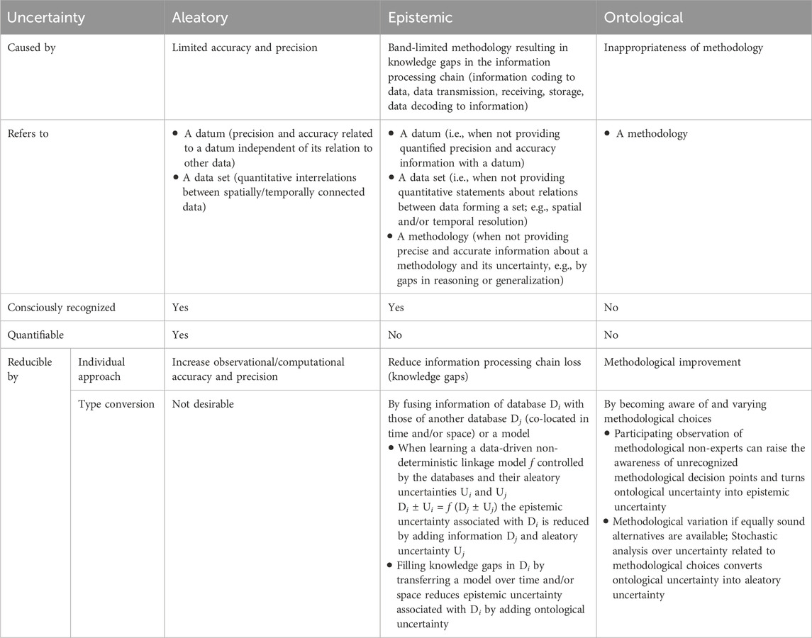
Table 1. Types of uncertainty (Asadi, 2023, modified).

We utilize a non-parametric multiple regression approach, specifically regression random forest (RF; e.g., Breiman, 2001), to regionalize CRNS SM data. To account for the aleatory uncertainty associated with the data, we use the RF regression within a Monte Carlo (MC) framework. This methodology is applied to a CRNS SM data set provided by a research institution and auxiliary data sourced from a science-based foundation and governmental authorities.

While both regression RF and MC methods are well-established, their application to probabilistic SM regionalization with full consideration of aleatory data uncertainty propagation is straightforward. However, our study highlights a significant challenge: the current practices of uncertainty communication by data providers hinder the seamless application of existing uncertainty quantification methodologies.

Despite these challenges, we successfully generate probabilistic SM maps that individually and jointly illustrate the contributions of aleatory uncertainty from both CRNS and auxiliary data sets to SM regionalization. Our findings not only pinpoint specific issues in the uncertainty communication practices of the data providers we utilized but also offer general recommendations for improving future uncertainty reporting. Since ontological uncertainty is not included in our analyses, our uncertainty quantification should be regarded as a potentially optimistic estimate. Nonetheless, it represents a more comprehensive approach than usually done and extends the work of Dega et al. (2023).

We begin by introducing the survey area, available data sets, and the uncertainty information provided. We detail and illustrate our methodology for incorporating data aleatory uncertainty into RF regressions within a MC framework. We critically evaluate our results, discuss the limitations of our uncertainty quantification, and finally propose recommendations to improve such analyses through enhanced uncertainty communication.

2 Study area and database

2.1 The Müglitz catchment and its vicinity

The Müglitz catchment is located in the federal state of Saxony, eastern Germany, covering an area of 209 km² (Figure 1a). The Müglitz river drains the eastern part of the Ore Mountains, flowing north from the German-Czech border into the Elbe River, south of the city of Dresden. The river originates in the Czech Republic at an altitude of 780 m and joins the Elbe at 113 m above sea level. It has a total length of approximately 50 km, with the first 400 m running through the Czech Republic.

Figure 1

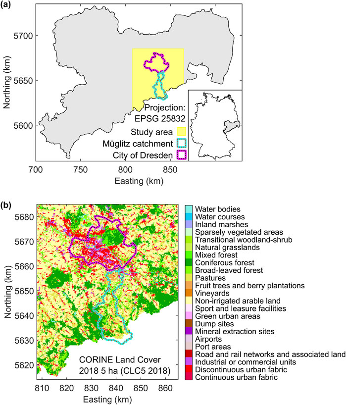
Figure 1. (a) The political boundaries of the federal state of Saxony, along with the study area, the contours of the Müglitz catchment, and the administrative boundaries of the City of Dresden. The inset map highlights Saxony’s location in eastern Germany. (b) CORINE land cover information with a minimal area size of 5 ha as provided by the Federal Agency for Cartography and Geodesy (BKG; https://gdz.bkg.bund.de/index.php/default/open-data/corine-land-cover-5-ha-stand-2018-clc5-2018.html, accessed 15 October 2024).

The landscape is characterized by expansive rolling plateaus and narrow valleys with steep slopes. More than 50% of the catchment consists of pastures and arable land on plateaus covered by thin soils. Around one-third of the area is forested (Figure 1b), primarily along the steep valley slopes.

The Müglitz catchment has been extensively studied in recent years (e.g., Tarasova et al., 2020; Hannemann et al., 2022; Rink et al., 2022; Wieser et al., 2023) as it is one of the intensive test sites within the Modular Observation Solutions for Earth Systems (MOSES) initiative (Weber et al., 2022). The Müglitz catchment and various data acquisition and modeling initiatives have been visualized in a virtual geographic environment, available at https://www.youtube.com/watch?v=plPEtkkR0pQ (last accessed 19 February 2025; Rink et al., 2022).

Our study area is bounded to the south by the German-Czech border and extends around the German section of the Müglitz catchment, which accounts for approximately 95% of the total Müglitz catchment (Figure 1). The survey area includes parts of the Ore Mountains and the Elbe Sandstone Highlands, situated west and east of the Müglitz catchment, respectively. North of the catchment, the city of Dresden lies within the Dresden Basin, a 10 km-wide valley of the Elbe River stretching northwest. The survey area also includes parts of the Lusatian Plateau to the north and the West Lusatian Hill Country and Uplands to the northeast.

2.2 The auxiliary data

2.2.1 Soil data

We use maps of physical and chemical soil state variables, including bulk density, sand fraction, clay content, and soil organic carbon, within the 5–15 cm depth range. The data are mapped on a regular grid with a 250 m node spacing, with gaps in urban areas. The soil data were obtained from www.soilgrids.org (accessed 15 October 2024), a service maintained by ISRIC–World Soil Information, an independent, science-based foundation.

The soil maps are generated using non-parametric multiple regression through quantile RFs, combining sparse soil profiles with multiple layers of densely mapped auxiliary data (Poggio et al., 2021). For each state variable, maps are provided for both the median (quantile q_0.5) and mean values at each grid node. Additionally, quantile maps for q_0.05 and q_0.95 define the lower and upper bounds of a 90% prediction interval. Corresponding maps are shown in Figure 2.

Figure 2

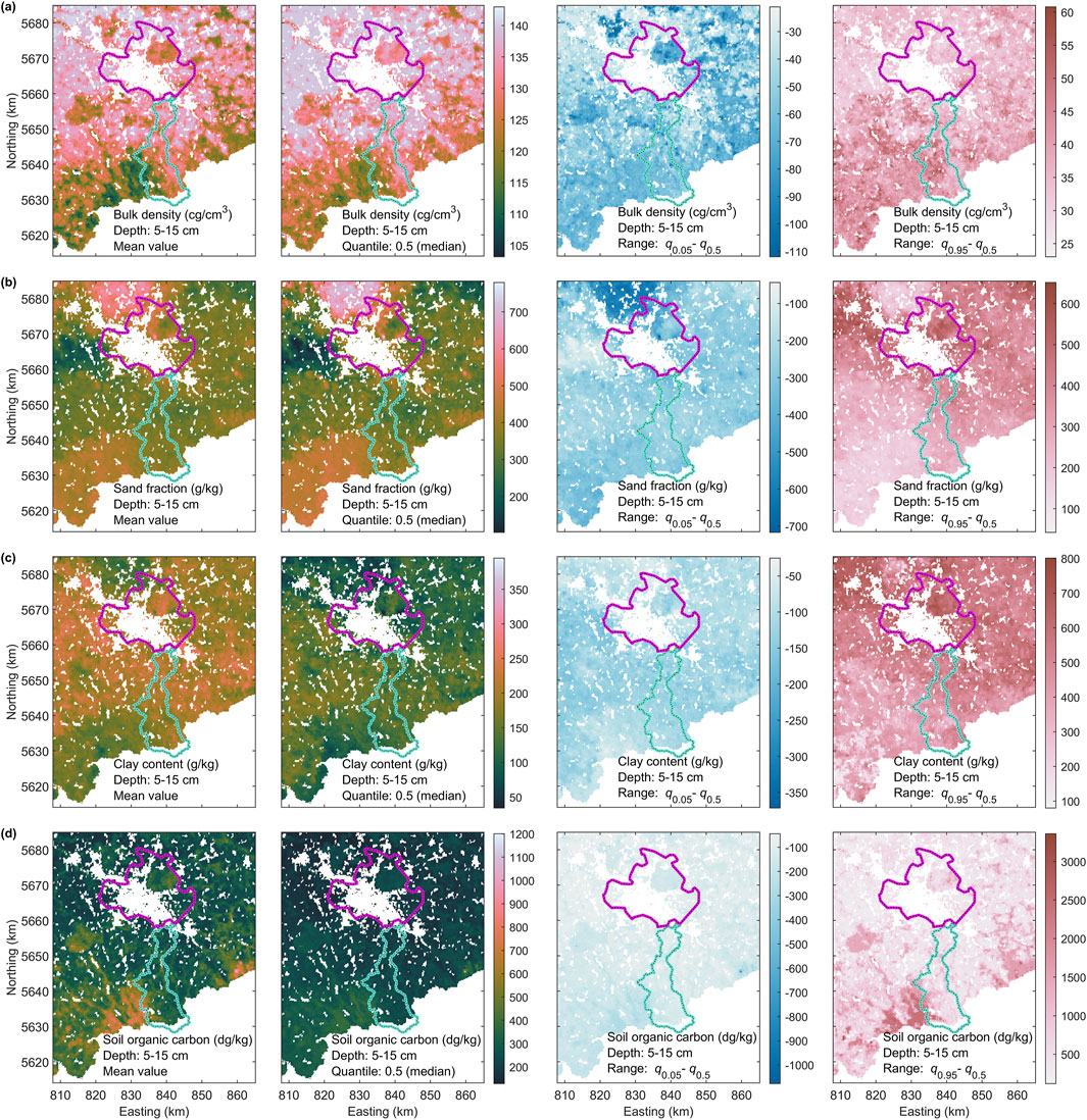
Figure 2. Median and mean soil maps for (a) Bulk density, (b) Sand fraction, (c) Clay content, (d) Soil organic carbon with a grid node spacing of 250 m. Additionally, for each data set ranges between quantiles q_0.5 and q_0.05 as well as q_0.95 and q_0.5 are shown which fully illustrates the information delivered by the data provider. For explanation of magenta and cyan polygons see Figure 1a.

An uncertainty map is also available, quantifying the ratio q_0.5/(q_0.95 - q_0.05). However, we do not display or use this uncertainty layer here, as it is a linear combination of the provided quantile maps and does not offer additional independent information. The quantile and mean maps in Figure 2 are sparse representations of probability density functions (PDFs) for each grid cell resultant from quantile RFs. Differences between mean and median maps indicate skewed PDFs. This is further supported by different absolute distances between q_0.05 and q_0.95 from q_0.5 (see, for example, Figure 2a).

2.2.2 Topographic data

In addition to the soil maps, we also obtained a digital terrain model with a 200 m grid spacing (DGM200), provided by the German Federal Agency for Cartography and Geodesy (BKG; https://gdz.bkg.bund.de/index.php/default/digitales-gelandemodell-gitterweite-200-m-dgm200.html, accessed 15 October 2024). According to the BKG, the positional precision/accuracy is ±5 m, while the elevation precision/accuracy is ±10 m (BKG, 2021). Note that in BKG (2021), the German word “Genauigkeit” is used, which does not distinguish between precision and accuracy. The DGM200 was derived from the DGM5 (a 5 m grid terrain model) by selecting the relevant grid points. The DGM5 data sets were originally generated by state surveying authorities and later merged by the BKG into a homogeneous, nationwide data set (BKG, 2021).

The Landesamt für Geobasisinformation Sachsen (GeoSN) is the state surveying authority for Saxony, where our survey area is located. According to GeoSN, their digital terrain models are produced according to product and quality standard for digital terrain models (AdV, 2021), established by the AdV (Working Group of Surveying Administrations of the Federal and State Governments). These models are derived through LiDAR data interpolation, and their elevation precision/accuracy matches that of the LiDAR data. The elevation uncertainty of the LiDAR data is given as ±0.15 m, representing two standard deviations (https://www.landesvermessung.sachsen.de/fachliche-details-8645.html, accessed 2 January 2025).

In AdV (2021), certain data sets are listed meeting the standards defining the product and quality characteristics of digital terrain models within the official German surveying system (ATKIS-DGM; AdV, 2021). Among the listed products are DGM5 data sets from the federal states and the DGM200 data set from the BKG. The elevation precision/accuracy of georeferenced raster elements in digital terrain models is specified as (i) flat to gently sloping, open terrain: ±10 cm + 5% of the raster width and (ii) steep terrain with dense vegetation: ±10 cm + 20% of the raster width.

For a 1 m grid terrain model (DGM1), this corresponds to ±0.15 m and ±0.3 m, depending on terrain slope and vegetation. For a DGM5, the expected uncertainty ranges from ±0.35 m to ±1.1 m, which is significantly higher than the ±0.15 m stated by GeoSN. Surveying authorities in other federal states report these higher uncertainty values for their DGM5 data sets, explicitly stating that they represent two standard deviations (e.g., https://www.lvermgeo.sachsen-anhalt.de/de/gdp-dgm-dom-lsa.html, accessed 2 January 2025). For the DGM200 from BKG, this method results in elevation uncertainty (two standard deviations) of ±10.2 m in flat open terrain and ±40.2 m in steep terrain with dense vegetation. It is explicitly stated, that the measurement values used as the basis for deriving the raster element position have positional inaccuracies, which are accounted for in the elevation accuracy specification of the raster element position, already. This would make an additional statement about position precision/accuracy as provided by the BKG for the DGM200 unnecessary. Figure 3 shows the DGM200 mapped on the same grid previously used for the soil data.

Figure 3

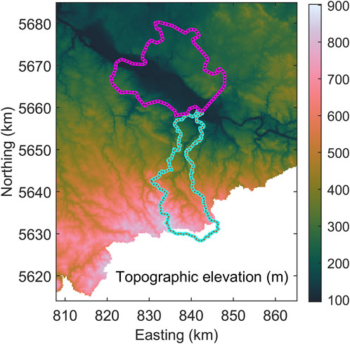
Figure 3. Digital Terrain model with 200 m node spacing mapped on the same grid as used for the maps in Figure 2.

2.3 The soil moisture data

CRNS measurements were conducted on 16 July 2019, between approximately 6:25 a.m. and 11:05 a.m. No precipitation was recorded in the survey area during this period. The system was mounted on a car (e.g., Schrön et al., 2018) that traveled along parts of the public road network within and near the Müglitz catchment (Figure 4a). The route was chosen as a compromise to cover large distances across the catchment in the short available time frame, and the driving speed was kept as constant as possible without compromising traffic safety or the driver’s well-being.

Figure 4

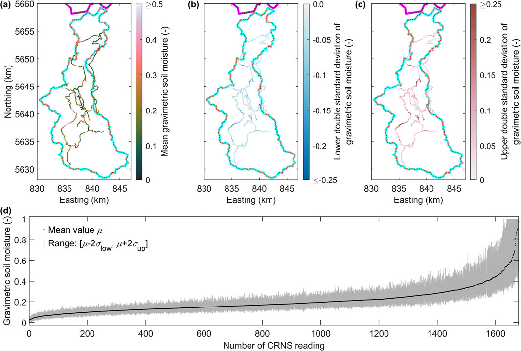
Figure 4. (a) Mean gravimetric soil moisture values derived from CRNS measurements and their corresponding (b) lower and (c) upper double standard deviations. For explanation of magenta line and cyan polygon see Figure 1a. (d) All 1,682 soil moisture data with their double standard deviation range sorted in ascending order. Note, that the upper standard deviation systematically exceeds the lower standard deviation. Standard deviations are clipped for high and low soil moisture values.

Neutron counts were integrated over 10-s intervals, resulting in 1,682 readings. As detailed in Dega et al. (2023), a non-linear function was used to convert the measured neutron counts into gravimetric SM. This processing skewed the normally distributed aleatory uncertainty of neutron count rates into asymmetric distributions. The uncertainty in gravimetric SM was characterized by merging the left- and right-hand sides of two different normal distributions at their common mean. This resulted in upper and lower standard deviations, σ_up and σ_low, respectively, associated with a mean value μ, which represents the measured gravimetric SM (Figures 4a–c). The upper standard deviation exceeded the lower one. For high mean values, the upper standard deviation was clipped to ensure that μ + 2σ_up ≤ 1. Similarly, μ - 2σ_low ≥ 0 (Figure 4d). While the lower cutoff credits a physical limitation, the motivation of the data provider for the upper cutoff appears empirical.

3 Methodology

Our methodology is summarized in the flowchart shown in Figure 5. We walk through the diagram by discussing the processing branches related to the auxiliary data and the soil moisture data separately. Please note that the final two steps in the flowchart (evaluation and visualization) correspond to the content presented in the Results and Discussion sections.

Figure 5

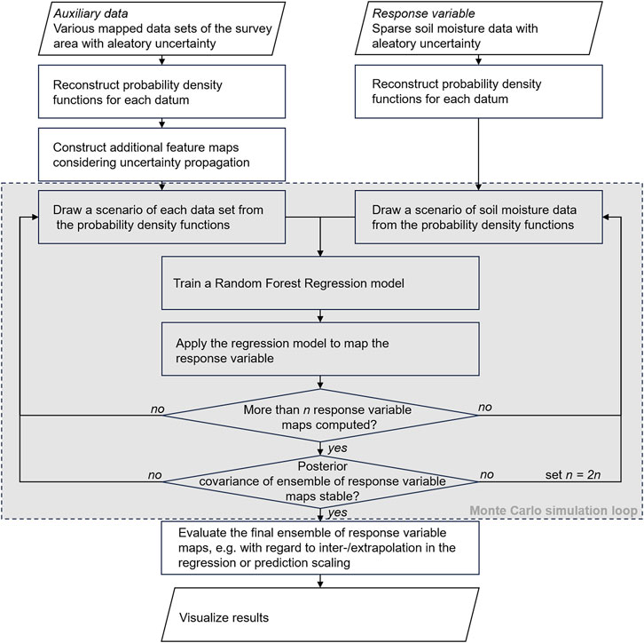
Figure 5. Flow chart of the data processing workflow.

3.1 Aleatory uncertainty in auxiliary soil data

The provided quantile and mean values for each map grid node offer a sparse representation of the PDFs derived from quantile RFs. To quantify the aleatory uncertainty at each grid node, we need to reconstruct the full PDF or its integral, the cumulative distribution function (CDF).

However, with only three given quantiles (q_0.05, q_0.5, and q_0.95) there are only three support points available for the PDF or its corresponding CDF. This introduces significant epistemic uncertainty in how these points should be connected, resulting in an infinite number of possible PDFs or CDFs. At this point the data provider does not match the requirements of aleatory uncertainty communication (Table 1). Consequently, this epistemic uncertainty makes it impossible to quantify aleatory data uncertainty based on the data alone.

However, we replace epistemic uncertainty with beliefs, converting it into ontological uncertainty (Table 1), which remains outside the scope of our subsequent analyses. To address this, we apply the philosophical principle known as Occam’s razor and determine that the points defining the CDF are connected by straight lines – the simplest point connectors according to our belief. Additionally, we determine lower and upper limits for the CDFs, setting them at 20 cg/cm³ and 200 cg/cm³, respectively, based on Panagos et al. (2024).

Since the CDF must satisfy not only the chosen limits and the three given quantiles but also the provided mean value, we formulate an optimization problem to find a suitable CDF. To maintain simplicity, we limit it to just two model parameters. These parameters represent additional points that help define the shape of the CDF beyond the given support points and chosen limits.

Figure 6 illustrates different setups for the bulk density of the central map grid node at 836.5 km East and 5,648 km North. To determine the optimal CDFs that meet the limits, support points, and mean value, we employ particle swarm optimization (PSO; Kennedy and Eberhart, 1995). Our swarm consists of 100 particles. We follow Tronicke et al. (2012) and chose an inertia weight of 0.7298 and cognitive and social learning rates of 1.4962. The algorithm terminates after 300 iterations or when the absolute difference between the measured and modeled mean value is less than 1e-9. We initialize the PSO four times and show the resulting solutions in Figure 6.

Figure 6

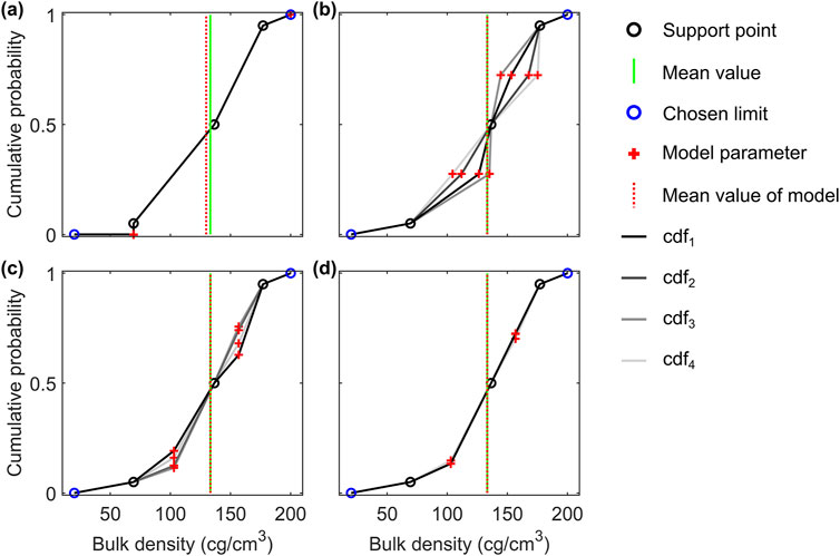
Figure 6. Cumulative distribution functions for the central map grid node in Figure 2a. (a-d) Solutions with different model parameters. For details see text.

In Figure 6a, we present the solutions obtained when allowing the model parameters to vary freely within the intervals (q₀, q_0.05) and (q_0.95, q₁). All four runs yield nearly identical results but fail to produce CDFs that match the given mean value. The model parameters tend to converge toward extreme solutions positioned at the edges of the permitted intervals.

To address this, we adjust the model setup by placing the model parameters at the midpoint between the given support points, allowing them to vary either horizontally or vertically (Figures 6b,c). All four runs produce CDFs that satisfy both the support points and the mean value. However, the resulting CDF shapes vary significantly, indicating the presence of multiple deep local optima that still provide a sufficient data fit.

To improve reproducibility, we introduce a penalty term to constrain the smoothness of the CDF and combine this with the setup shown in Figure 6c. This adjustment leads to more stable solutions (Figure 6d), ensuring reasonable reproducibility while still maintaining consistency with the given mean value.

We apply this setup to compute bulk density CDFs for each grid node, achieving solutions where the mismatch between measured and modeled mean values remains below 2e-7. Similarly, we extend this approach to sand fraction, clay content, and soil organic carbon data, as shown in Figure 2. Through empirical analysis, we determine the lower limits to be 0.7⋅q_0.05, 0.5⋅q_0.05, and 0.5⋅q_0.05, respectively. The upper limits for all three data sets are set to 1.3⋅q_0.95.

3.2 Aleatory uncertainties in auxiliary topographic data

By providing a central value and a double standard deviation, the shape of the PDF is well-defined as a normal distribution, with its model parameters fully specified. However, the standard deviation is not explicitly given for each map grid node. Instead, it is differentiated into two distinct values based on topographic slope and dense vegetation cover. The actual function governing this differentiation is only described qualitatively using definitions such as “flat to gently sloping, open terrain” and “steep terrain with dense vegetation”. However, no quantitative details are provided regarding the transition between these categories or how slope and vegetation precisely influence the double standard deviation. This epistemic uncertainty requires filling the knowledge gap with a methodology that relies more on beliefs than on concrete knowledge and fails to provide quantitative data uncertainty statements (Table 1). As a result, epistemic uncertainty is replaced with ontological uncertainty, which remains outside the scope of subsequent analyses.

Furthermore, there is uncertainty regarding how to integrate the uncertainty information provided by BKG (2021) and AdV (2021), both of which are claimed to apply to the DGM200. Additionally, no clarification is given on how accuracy and precision contribute to the reported double standard deviations. Paasche and Schröter (2023) demonstrated that spatial noise fields following a normal distribution, with varying spatial correlation wavelengths but the same mean and double standard deviation, can be applied to digital terrain data while still adhering to the given uncertainty definitions. However, the way these noise fields propagate through subsequent analyses differs.

Due to the lack of information about spatial uncertainty correlation, we address this epistemic uncertainty by assuming no correlation between grid nodes. Treating double standard deviations in the range of [10.2, 40.2] m as spatially uncorrelated uncertainty in the digital terrain model would lead to topographic slopes and aspects that are largely random, which would generally question the value of the DGM200. To mitigate this, we lower the maximum accepted double standard deviation to 10 m, following BKG (2021), assuming this value represents a maximal spatially uncorrelated uncertainty.

When computing PDFs for each map grid node of the digital terrain model, we interpret “dense vegetation” as forest. Using CORINE land cover data (Figure 1b), we derive a binary mask F that classifies mixed forest, coniferous forest, and broad-leaved forest as areas of dense vegetation within the survey region (Figure 7a).

Figure 7

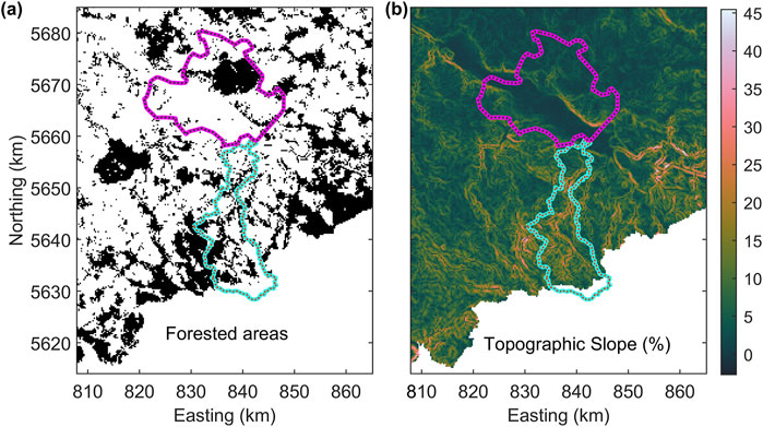
Figure 7. (a) Binary mask derived from the land cover data in Figure 1b. Black regions depict forested areas. (b) Topographic slope map derived from the Map in Figure 3. For explanation of magenta and cyan polygons see Figure 1a.

Additionally, we generate a topographic slope map S of the survey area (Figure 7b) from the digital terrain model (Figure 3), applying a deterministic approach. We define an empirical mixing model that combines slope and dense vegetation to compute the elevation uncertainty u_j for the jth map grid node

$u_j=u_{0j}+u_{Fj}+u_{Sj}.(1)$

u_0j is the base uncertainty for the jth grid node referring to open flat terrain and defined as

$u_{0j}=r_j·{\sigma }_0,(2)$

with r_j being a random number drawn from the standard normal distribution and σ₀ being the standard deviation of 1.5 m u_Fj is the forest related uncertainty determined as

$u_{\mathrm{F}j}={\sigma }_{\mathrm{F}}·f_j·\left\{\begin{array}{cc}-1& if{r}_j<1\\ 1& else\end{array}\right.(3)$

with σ_F = 4 m and f_j ∈ F. u_Sj is the slope related uncertainty

$u_{\mathrm{S}j}=r_j·{\sigma }_1·d_j,(4)$

with σ₁ = 1.5 m d_j realizes a slope related scaling by

$d_j=\min \left\{1,\frac{s_j}{s_L}\right\},(5)$

with s_j ∈ S and s_L = 50%. Using Equations 1–5, we can discretely sample the PDFs for each grid node of the digital terrain model, assuming no spatial correlation, and compute the mean elevation values along with their corresponding standard deviations (Figure 8a). The standard deviations σ₀, σ_F, and σ_S are empirically chosen and preserve the ratio given by the data provider that σ_F+σ_S ≈ 4⋅σ₀ for steep forested terrain. The resultant mean double standard deviation of the map is approximately 8 m and falls slightly below the assumed maximal uncorrelated double standard deviation of 10 m.

Figure 8

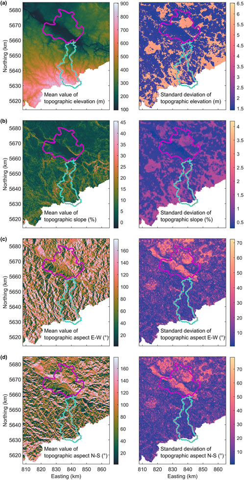
Figure 8. Mean maps and corresponding standard deviations of topographic (a) elevation (b) slope, and aspect split into its sine and cosine components representing its (c) east-west and (d) north-south components.

By randomly sampling from these PDFs, we derive probabilistic topographic slope and aspect information, as well as their associated standard deviations. These additional topographic data sets, together with topographic elevation and the soil maps, serve as auxiliary data in our multiple regression analysis. Since RF regression assumes that data are projected on a linear axis, we transform the circular topographic aspect information by splitting it into its sine and cosine components, representing the east-west and north-south aspect directions, respectively (Figures 8b–d).

3.3 CRNS data uncertainty and its relation to the information fusion methodology

The 1,682 soil moisture readings fall within 419 map grid cells of the auxiliary data, with the number of readings per grid cell varying. We merge the PDFs of gravimetric SM for each grid cell.

Since the gravimetric SM PDFs are defined by a mean value and lower and upper standard deviations, merging them requires linking two normal distributions with different standard deviations at their common mean value. One approach is to generate continuous, smooth, skewed PDFs, as shown in Figure 9a. However, in these skewed distributions, the mean value no longer aligns with the most likely value, which was initially the common mean of the two individual normal distributions.

Figure 9

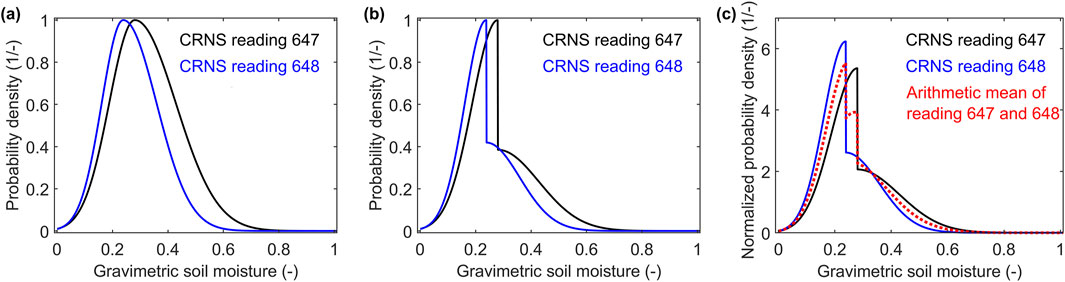
Figure 9. Probability density distributions of the soil moisture data falling with the map grid cell centered at 834,25 km East and 5,637.25 km North (blue and black lines). (a) Equal scaling of upper and lower standard deviation. (b) and (c) Weighted upper and lower standard deviation so that the center value corresponds to the mean value of each distribution. The red dotted line in (c) is the arithmetic mean of the blue and black curve representing the integrated soil moisture PDF for this grid cell.

To preserve the given definition, where PDFs are characterized by a mean value and two distinct standard deviations, we scale the left and right sides of the common distributions differently. This results in discontinuous, non-smooth PDFs at their mean value, as seen in Figure 9b which are outside the strict definitions of distributions reasonably described by mean values and standard deviations. However, their mean values and lower and upper standard deviations can be computed anyway and remain consistent with the provided data. The blue curve in Figure 9b represents a more concentrated distribution than the black curve, indicating lower uncertainty. To account for this reduced uncertainty, we scale both PDFs so that the area under each curve remains equal (Figure 9c). By summing the scaled PDFs, we obtain an integrated PDF that quantifies gravimetric SM uncertainty for the grid cell based on all CRNS measurements falling therein.

3.4 Random forest regression and Monte Carlo sampling

We use multiple nonlinear regression (e.g., Howarth, 2001; Kleinbaum et al., 2013) to regionalize the sparse soil moisture data. This method relates a one-dimensional response variable (also referred to as dependent variable, target variable, label data), y (size m × 1), to a densely sampled multi-dimensional predictor (also referred to as independent variable, feature data, explanatory variable), X (size n × t), where t = 8 is the number of vectorized auxiliary data sets (Figures 2, 8) available at n co-located map grid cells.

To set up a multiple regression of the form y = g (X, U) (Arens et al., 2015), SM data must be available for m grid cells. U is a disturbance matrix capturing uncertainty in X and y. Here, we limit it to aleatory uncertainty.

With m co-located pairs of X and y, we compute a regression model g by means of regression RF to estimate SM across all n nodes. To account for U, we embed the regression in a Monte Carlo framework, repeatedly sampling m co-located data sets from y and X along with their PDFs or CDFs. A regression model is then computed for each sampled pair of y and X.

To determine a regression model g, we use a RF algorithm (Breiman, 2001), that makes no assumptions about the model’s form. As with any regression method, g depends on parameter choices, including numerical settings (e.g., the number of trees) and conceptual decisions (e.g., the objective function). Ontological uncertainty associated with these choices is not part of our analyses.

We generate bootstrapped data sets using replacement sampling (Horowitz, 2019), with an in-bag fraction of 0.66. At each tree split, the optimal predictor is selected from two randomly chosen auxiliary data sets in X. In some cases, the best results were obtained using only one randomly selected auxiliary variable when combined with more than 500 trees, suggesting a relatively noisy database.

Of the 419 map grid nodes with available soil moisture data, 64 were excluded due to missing auxiliary information, leaving 355 nodes. These were divided into a learning set (m = 319) and a test set (m^* = 36), with the test set held out from model training. To ensure a fair comparison with interpolated (and not extrapolated) predictions, the test set includes only map nodes within the convex hull of the m learning nodes in predictor space.

Settings were chosen based on empirical testing of the first 10 Monte Carlo samples considering the aleatory uncertainty of y and X. Figure 10a shows the mean squared error as a function of the minimum allowed leaf size. Since we do not impose a fitting limit, the random forest likely overfits when using a minimal leaf size of 1. However, as results for leaf sizes of 1 and 2 largely overlap, we select a minimum leaf size of 5. Stable solutions are achieved when the random forest consists of 200 trees (Figure 10a).

Figure 10

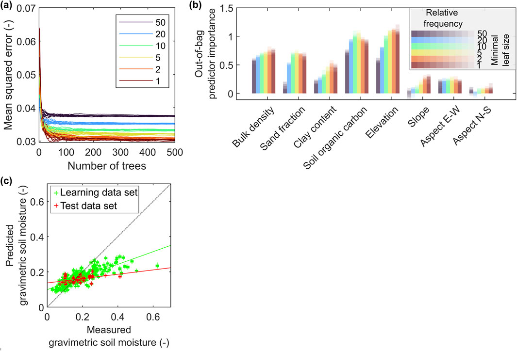
Figure 10. (a) Mean squared error of RF regression over the number of trees in the RF for 10 repeated runs with random initialization and different minimal leaf node sizes between 1 and 50 for the same MC realization of predictor and response variable. (b) Importance of the auxiliary data sets in Figures 2, 7 as predictors in the RF runs illustrated in (a). (c) Scatter plot of predicted vs. measured soil moisture values for 10 randomly initialized runs with minimal leaf size of 5. Solid green and red lines indicate linear models optimally fitting learning and test data.

The relative importance of predictors depends on the degree of data fitting, which is controlled by the minimum leaf size (Figure 10b). Topographic slope and aspect have low importance when the minimum leaf size is set to 5. However, aspect data contribute positively when the minimum leaf size is increased to 50, suggesting their relevance at early tree splits. In contrast, variables like sand fraction gain importance later in the tree growth process, primarily during fine-tuning at deeper splits.

Since auxiliary data sets that are rarely used in splitting decisions contribute minimally to the uncertainty of the random forest regression model, we do not discard them a priori. Feature importance varies with Monte Carlo sampling of y and X, meaning a strict cutoff would introduce ontological uncertainty and could lead to the unintended exclusion of useful predictors in some Monte Carlo runs.

Figure 10c presents a scatter plot of predicted versus measured soil moisture. The predicted values show a reduced range, indicating imperfect leaf separation and significant scattering within the leaves, which suggests a noisy database. The slopes of linear models fitted to the measured and predicted data are clearly lower than 1 (Table 2).

Table 2

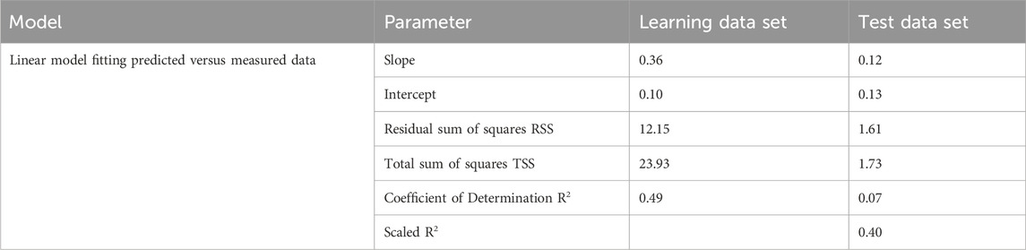
Table 2. Parameters of a linear model fitting predicted versus measured soil moisture data. The linear model has been fitted to the results of the first 10 Monte Carlo runs.

For the learning data, the coefficient of determination ($R_{\mathrm{L}}^2$ = 0.49; Table 2) indicates moderate explanatory power, suggesting some variance remains unexplained by the model. Speculating, this might again possibly indicate noisy data and might have improved when additionally considering meteorological variables, such as precipitation, that are known to influence soil moisture. For the test data set, $R_{\mathrm{T}}^2$ = 0.07, which suggests a poor model. However, directly comparing both R² values is not entirely fair, as the test data set has a significantly reduced range due to the selection of points only within the convex hull, meaning for the total sum of squares TSS_T << TSS_L.

The aleatory uncertainty in the test data should be comparable to that in the learning set (and therefore also their normalized residual sum of squares RSS_T and RSS_L) unless there is a systematic correlation with the convex hull in the predictor space, which we did not find. When scaling the RSS_T by multiplication with m/m^* to account for the smaller size of the test sample, we get RSS_Tscaled = 14.27, slightly higher than RSS_L = 12.15. This confirms a lower performance for the regression model on the test data set when relating RSS_Tscaled and TSS_L, resulting in a scaled $R_{\text{Tscaled}}^2$ = 0.4, which still suggests moderate performance, albeit weaker than for the learning data.

We continuously perform MC sampling, generating regression models for each pair of y and X by randomly drawing from their probability density functions (PDFs). These models are then applied to compute gravimetric SM maps. To assess the representativeness of the generated ensemble, we conduct an a posteriori correlation analysis (Tronicke et al., 2012, particularly Equations 3–5 therein). Specifically, we randomly select 1,000 grid nodes and calculate the grid node correlation matrix over a set of SM maps. Figures 11a,b present the correlation matrices P₁₉ and P₁₉₄₅₆, corresponding to the first 50 of the 1,000 selected grid nodes, calculated over 19 and 19,456 SM maps, respectively. While P₁₉ displays a seemingly random mix of positive and negative correlations, P₁₉₄₅₆ reveals more systematic patterns, with some grid nodes showing consistently positive correlations and others showing little to no correlation, but almost no negative correlations. The positive correlations occur because certain grid nodes are frequently assigned to the same leaf, regardless of MC sampling variations.

Figure 11

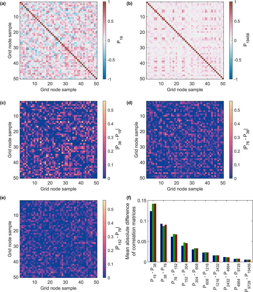
Figure 11. Soil moisture grid node correlation matrices (P₁₉ and (b) P₁₉₄₅₆ calculated for 50 grid nodes over ensembles of 19 and 19,456 soil moisture maps achieved by MC regression RF considering uncertainty in y and X, respectively. (c–e) Differences in correlation matrices (a) P_1_9 and (b) P_1_9_4_5_6 calculated for ensembles comprising different numbers of soil moisture maps. (f) Mean absolute differences of correlation matrices comprising different number of soil maps. Blue, green, and red bars refer to ensembles (i) ignoring uncertainty in X, (ii) ignoring uncertainty in y, and (iii) considering uncertainty in y and X, respectively. For explanation of y and X see text.

Figures 11c–e illustrate the differences between correlation matrices computed from pairs of SM map subsets. For each comparison, the number of maps used to compute the correlation matrices is doubled. As the ensemble size increases, differences between correlation matrices diminish, indicating increasing statistical stability of the ensemble (see red bars in Figure 11f). We extend our computations to an ensemble of 20,000 soil moisture maps, ultimately achieving a mean absolute correlation matrix difference of 0.0057.

Following the procedure outlined above, we generate additional ensembles of soil moisture maps, each accounting for different sources of uncertainty. One ensemble is computed while ignoring the aleatory uncertainty in the soil moisture data (y), and another while ignoring the uncertainty in the auxiliary data (X). For ensemble sizes of 20,000 soil moisture maps, the mean absolute differences between correlation matrices remain below 0.006, confirming the statistical stability of the results (Figure 11f).

4 Results

Figure 12 depicts the computed SM maps. Figure 12a shows the deterministic solution, where aleatory uncertainty in the CRNS SM (y) and auxiliary (X) data is ignored. Since no MC sampling was performed, this approach does not provide quantified uncertainty estimates for the map.

Figure 12

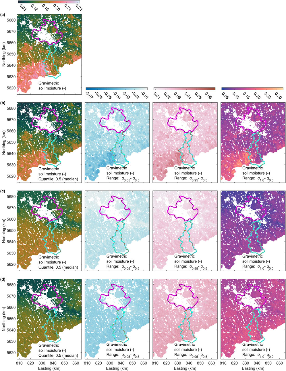
Figure 12. (a) Deterministic soil moisture map achieved by regression RF ignoring uncertainty in y and X. (b–d) Median (q_0.5) soil moisture maps and three corresponding quantile ranges describing ensembles of 20,000 soil moisture maps computed using MC regression random forest when (i) ignoring uncertainty in X, (ii) ignoring uncertainty in y, and (iii) considering uncertainty in y and X, respectively. For explanation of y and X see text. For explanation of magenta and cyan polygons see Figure 1a.

Figures 12b,c illustrate the results from 3 MC ensembles (i) ignoring uncertainty in X, (ii) ignoring uncertainty in y, and (iii) considering uncertainty in both y and X, respectively. For each ensemble, we display the q_0.5 map, which represents the median soil moisture value at each grid node. This is supplemented with percentile ranges, showing the spread between q_0.5 and q_0.05, q_0.95 and q_0.5, and q_1.0 and q_0.0 to provide a sense of uncertainty in the soil moisture distribution.

The overall pattern in the deterministic and q_0.5 soil moisture maps (Figures 12a,b) is similar. The lowest soil moisture values are observed in the Dresden Basin, extending from the center of the map toward the northwest. In contrast, the highest values appear in the southwest, aligning with the high-elevation areas of the Ore Mountains. Since both maps were generated ignoring the aleatory uncertainty in the auxiliary data, their only difference is that the q_0.5 map (Figure 12b) incorporates the uncertainty of the soil moisture data, whereas the deterministic map does not. The q_0.5 map also exhibits a slightly damped amplitude compared to the deterministic map. The percentile range maps in Figure 12b reveal a clear positive correlation between uncertainty and SM values. This reflects the propagation of aleatory uncertainty in the SM data, which is itself correlated with SM levels (see Figure 4d).

When aleatory uncertainty in the auxiliary data is considered, the pattern of the q_0.5 SM map changes. The previously distinct high soil moisture area in the southwest becomes more uniform, merging into a broader region of elevated soil moisture across the mountainous and hilly areas. The corresponding uncertainty distribution is also smoother and shows a slight correlation with topographic elevation. However, the sharp spatial variations in uncertainty seen in the topographic data (caused by vegetation differences) or in certain soil maps (see Figures 2, 8) are largely smoothed out.

When both SM and auxiliary data uncertainties are included, the percentile ranges further increase, leading to an even smoother representation. Simultaneously, the q_0.5 SM map’s amplitude is further damped. Across much of the study area, the 90% prediction interval (q_0.05 q_0.95) does not fall below 0.06. Given that median SM values mostly range between 0.1 and 0.18, this suggests that, with propagated aleatory uncertainty, the SM regionalization can reliably distinguish only broad wet and dry conditions, while finer-scale differentiation remains highly uncertain.

5 Discussion

Considering aleatory uncertainty in the auxiliary data can alter the spatial pattern of median SM. As aleatory uncertainty increases, the risk of regression shrinkage also grows, often due to imperfect node separation or high variability within leaves. MC sampling does not help mitigating this, resulting in median SM maps with reduced amplitude. However, when interpreted alongside their corresponding uncertainty estimates, these maps still provide some insights while minimizing the risk of overinterpretation.

Addressing this amplitude reduction is challenging. A straightforward approach is to apply a posteriori scaling, adjusting the SM maps by computing an optimal linear correction model for each map in the ensemble based on the match between predicted and measured SM. Figure 13a demonstrates this method for the ensemble that includes aleatory uncertainty in both y and X (Figure 12d). While this adjustment increases the range of the median map and its uncertainty bounds, it also introduces negative SM values in approximately 27% of the grid nodes, primarily affecting the Dresden Basin and the Lusatian Plateau in the north.

Figure 13

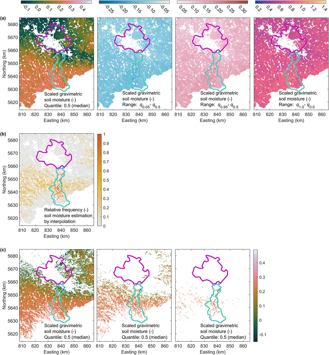
Figure 13. (a) The same as in Figure 12d but scaled to match the measured gravimetric data optimally. (b) Relative frequency of interpolating the RF regression model to achieve a soil moisture estimation for a map grid node. (c) The same scaled q_0.5 gravimetric soil moisture map as in Figure 13a with regions corresponding to relative frequencies >0, >0.1 and >0.5. For explanation of magenta and cyan polygons see Figure 1a.

For each map in the ensemble, we assess which grid nodes fall inside the convex hull of the predictor space defined by the learning data set. Grid nodes inside the convex hull require interpolation, while those outside require extrapolation, introducing increased ontological uncertainty - a factor not captured in our quantitative uncertainty propagation. Figure 13b illustrates the relative frequency of each grid node being inside the convex hull. The results indicate that our SM data set is not representative for certain areas, particularly the Dresden Basin and the Lusatian Plateau at the northern edge of the map, as these regions consistently require extrapolation. Beyond the sampling locations and their immediate surroundings, relative frequencies rarely exceed 0.5, suggesting that extrapolation dominates across most of the survey area.

We use the data shown in Figure 13b to generate binary masks, which are then overlaid on the median soil moisture map in Figure 13a. The binarization process uses increasing thresholds of >0, >0.1, and >0.5. As the threshold increases, larger regions of the survey area are blanked out (Figure 13c).

When grid nodes requiring 100% extrapolation are excluded, the fraction of grid nodes with negative SM values is reduced to 7.5%. The Dresden Basin and Lusatian Plateau in the northern part of the map are now blanked out. With thresholds >0.1 and >0.5, the fraction of negative values decreases further to 0.6% and 0.3%, respectively. This illustrates that the problem is largely due to ontological uncertainty, by applying our SM data to regions where they are not representative. For a threshold >0.1, even the northern and southern parts of the Müglitz catchment are no longer covered, raising questions about the representativeness of the CRNS survey for this area which was a major survey goal under the MOSES activities. Focusing only on areas where interpolation dominates reduces the mapped coverage to only 1.8% of the grid nodes, representing a very sparse sample of SM data across the survey area.

In future CRNS surveys, we recommend enhancing the information return of the CRNS data set by analyzing the predictor variables intended for regionalization prior to data acquisition. Schröter et al. (2015) successfully demonstrated that such preparatory efforts can result in highly efficient sparse sampling schemes with substantial information gain. However, in the case of mobile CRNS data acquisition, the selection of sampling locations is constrained by the road network, which might limit the efficiency of any optimized sampling design compared to those reported by Schröter et al. (2015).

6 Conclusion

We used regression RF embedded within a MC approach to propagate aleatory uncertainty from densely sampled auxiliary data sets and sparse gravimetric SM data into regionalized SM maps. However, method-inherent ontological uncertainty, such as uncertainties regarding the general suitability of our regression and MC methodology, falls outside the scope of our analysis and is assumed to overlay the considered aleatory uncertainty.

Despite the straightforward nature of our methods, the quantified uncertainties in our SM maps remain only estimates with unquantified residual uncertainty. Nonetheless, our results demonstrate that uncertainties in both response and predictor variables can significantly influence regionalized soil moisture and exhibit distinct spatial patterns. A true uncertainty quantification was not possible due to epistemic uncertainty in the communication of auxiliary data providers. This forced us to fill knowledge gaps with assumptions, introducing additional ontological uncertainty and ultimately preventing a purely quantified propagation of aleatory data uncertainty.

Problems arose due to the data providers’ insufficient consideration of the aleatory uncertainty associated with the data sets. The providers of soil maps and topographic data did not quantify the spatial relationships within their maps, requiring us to fill this gap, e.g., by assuming spatially uncorrelated uncertainty. Although the soil maps included quantitative uncertainty information for each datum, the provided uncertainty data were so sparse that we had to make additional assumptions about the smoothness of the PDFs. The topographic data, on the other hand, were supplied with well-defined PDF shapes assumed to follow normal distributions, but not at a datum-specific level. Instead, qualitative statements regarding uncertainty were provided based on slope and vegetation, leaving it to the user to determine how to apply them quantitatively. Had both data providers accounted for the nature of aleatory uncertainty (Table 1), they could have supplied quantitative uncertainty estimates for each datum as well as for the spatial relationships within their data sets. This would have made a study like the present one more straightforward and resulted in more realistic aleatory uncertainty quantification for the regionalized soil moisture maps. If simple models cannot be used to quantify aleatory uncertainty at the datum and data set levels, e.g., such as parameters of a normal distribution and a global (direction-dependent) frequency spectrum quantifying spatial data interrelations, respectively, a practical alternative would be to provide a set of maps that representatively sample aleatory uncertainty in a Monte Carlo framework.

Data availability statement

The raw data supporting the conclusions of this article will be made available by the authors, without undue reservation.

Author contributions

HP: Software, Methodology, Writing – original draft, Formal Analysis, Visualization, Conceptualization. SD: Formal Analysis, Methodology, Conceptualization, Writing – review and editing. MS: Formal Analysis, Data curation, Software, Conceptualization, Writing – review and editing, Funding acquisition. PD: Writing – review and editing, Conceptualization, Project administration, Supervision.

Funding

The author(s) declare that financial support was received for the research and/or publication of this article. CRNS measurement campaigns were conducted with support from the Helmholtz Association within the framework of MOSES. MS was supported by the Deutsche Forschungsgemeinschaft (DFG grant 357874777; research unit FOR 2694, Cosmic Sense II).

Acknowledgments

We thank Uta Ködel and Andreas Schoßland for organizing and conducting the CRNS measurement campaign.

Conflict of interest

Authors HP, SD, MS, and PD were employed by UFZ – Helmholtz Centre for Environmental Research GmbH.

Generative AI statement

The author(s) declare that no Generative AI was used in the creation of this manuscript.

Publisher’s note

All claims expressed in this article are solely those of the authors and do not necessarily represent those of their affiliated organizations, or those of the publisher, the editors and the reviewers. Any product that may be evaluated in this article, or claim that may be made by its manufacturer, is not guaranteed or endorsed by the publisher.

References

AdV (2021). Produkt-und Qualitätsstandard für Digitale Geländemodelle Version 3.2. Bearbeitungsstand 22.12.2021. Arbeitsgemeinschaft Vermessungsverwaltungen der Länder der Bundesrepublik Deutschland (AdV).

Google Scholar

Altdorff, D., Oswald, S. E., Zacharias, S., Zengerle, C., Dietrich, P., Mollenhauer, H., et al. (2023). Toward large-scale soil moisture monitoring using rail-based cosmic ray neutron sensing. Water Resour. Res. 59, e2022WR033514. doi:10.1029/2022wr033514

CrossRef Full Text | Google Scholar

Arens, T., Hettlich, F., Karpfinger, C., Kockelkorn, U., Lichtenegger, K., and Stachel, H. (2015). Mathematik. Springer.

Google Scholar

Asadi, J. (2023). “UQ in Earth science data,” in Uncertainty quantification dictionary. The helmholtz UQ community. Editors M. Frank, C. Fuchs, and B. Zeller-Plumhoff Available online at: https://dictionary.helmholtz-uq.de/content/types_of_uncertainty_overview.html (Accessed February 26, 2025).

Google Scholar

Babaeian, E., Sadeghi, M., Jones, S. B., Montzka, C., Vereecken, H., and Tuller, M. (2019). Ground, proximal, and satellite remote sensing of soil moisture. Rev. Geophys. 57, 530–616. doi:10.1029/2018rg000618

CrossRef Full Text | Google Scholar

Beven, K. (2016). Facets of uncertainty: epistemic uncertainty, nonstationarity, likelihood, hypothesis testing, and communication. Hydrological Sci. J. 61, 1652–1665. doi:10.1080/02626667.2015.1031761

CrossRef Full Text | Google Scholar

BKG (2021). Dokumentation digitales geländemodell gitterweite 200 m DGM200. Stand 17.03.2021. Berlin: Bundesamt für Kartographie und Geodäsie.

Google Scholar

Breiman, L. (2001). Random forests. Mach. Learn. 45, 5–32. doi:10.1023/a:1010933404324

CrossRef Full Text | Google Scholar

Brown, W. G., Cosh, M. H., Dong, J., and Ochsner, T. E. (2023). Upscaling soil moisture from point scale to field scale: toward a general model. Vadose Zone J. 22, e20244. doi:10.1002/vzj2.20244

CrossRef Full Text | Google Scholar

Chrisman, B., and Zreda, M. (2013). Quantifying mesoscale soil moisture with the cosmic-ray rover. Hydrology Earth Syst. Sci. 17 (12), 5097–5108. doi:10.5194/hess-17-5097-2013

CrossRef Full Text | Google Scholar

Dega, S., Dietrich, P., Schrön, M., and Paasche, H. (2023). Probabilistic prediction by means of the propagation of response variable uncertainty through a monte carlo approach in regression random forest: application to soil moisture regionalization. Front. Environ. Sci. 11, 1009191. doi:10.3389/fenvs.2023.1009191

CrossRef Full Text | Google Scholar

Desilets, D., Zreda, M., and Ferré, T. P. A. (2010). Nature’s neutron probe: land surface hydrology at an elusive scale with cosmic rays. Water Resour. Res. 46, W11505. doi:10.1029/2009wr008726

CrossRef Full Text | Google Scholar

Fersch, B., Jagdhuber, T., Schrön, M., Völksch, I., and Jäger, M. (2018). Synergies for soil moisture retrieval across scales from airborne polarimetric SAR, cosmic ray neutron roving, and an in situ sensor network. Water Resour. Res. 54, 9364–9383. doi:10.1029/2018wr023337

CrossRef Full Text | Google Scholar

Gault, J. A., and Albaraghtheh, T. (2023). “Types of uncertainty: overview,” in Uncertainty quantification dictionary. The helmholtz UQ community. Editors M. Frank, C. Fuchs, and B. Zeller-Plumhoff Available online at: https://dictionary.helmholtz-uq.de/content/types_of_uncertainty_overview.html (Accessed February 26, 2025).

Google Scholar

Hannemann, M., Nixdorf, E., Kreck, M., Schoßland, A., and Dietrich, P. (2022). Dataset of hydrological records in 5 min resolution of tributaries in the Mueglitz River basin Germany. Data Brief 40, 107832. doi:10.1016/j.dib.2022.107832

PubMed Abstract | CrossRef Full Text | Google Scholar

Heistermann, M., Francke, T., Schrön, M., and Oswald, S. E. (2021). Spatio-temporal soil moisture retrieval at the catchment scale using a dense network of cosmic-ray neutron sensors. Hydrology Earth Syst. Sci. 25, 4807–4824. doi:10.5194/hess-25-4807-2021

CrossRef Full Text | Google Scholar

Horowitz, J. L. (2019). Bootstrap methods in econometrics. Annu. Rev. Econ. 11, 193–224. doi:10.1146/annurev-economics-080218-025651

CrossRef Full Text | Google Scholar

Howarth, R. J. (2001). A history of regression and related model-fitting in the earth sciences (1636-2000). Nat. Resour. Res. 10, 241–286. doi:10.1023/a:1013928826796

CrossRef Full Text | Google Scholar

Jakobi, J., Huisman, J. A., Schrön, M., Fiedler, J., Brogi, C., Vereecken, H., et al. (2020). Error estimation for soil moisture measurements with cosmic ray neutron sensing and implications for rover surveys. Front. Water 2, 10. doi:10.3389/frwa.2020.00010

CrossRef Full Text | Google Scholar

JCGM (2008a). Evaluation of measurement data – guide to the expression of uncertainty in measurement. Joint committee for guides in metrology. JCGM 100, 2008.

Google Scholar

JCGM (2008b). Evaluation of measurement data – supplement 1 to the “Guide to the Expression of Uncertainty in Measurement” – propagation of distributions using Monte Carlo method. Joint Comm. Guid. Metrology, JCGM 101, 2008.

Google Scholar

Kennedy, J., and Eberhart, R. C. (1995). “Particle swarm optimization,” in Proceedings of the IEEE International Joint Conference on Neural Networks, Perth, WA, Australia, 27 November 1995 - 01 December 1995 (IEEE), 1942–1948.

CrossRef Full Text | Google Scholar

Kiureghian, A. D., and Ditlevsen, O. (2009). Aleatory or epistemic? Does it matter? Struct. Saf. 31, 105–112. doi:10.1016/j.strusafe.2008.06.020

CrossRef Full Text | Google Scholar

Kleinbaum, D. G., Kupper, L. L., Nizam, A., and Rosenberg, E. S. (2013). Applied regression analysis and other multivariable methods. Boston, MA: Cengage Learning.

Google Scholar

Köhli, M., Schrön, M., Zreda, M., Schmidt, U., Dietrich, P., and Zacharias, S. (2015). Footprint characteristics revised for field-scale soil moisture monitoring with cosmic-ray neutrons. Water Resour. Res. 51, 5772–5790. doi:10.1002/2015wr017169

CrossRef Full Text | Google Scholar

Lane, D. A., and Maxfield, R. R. (2005). Ontological uncertainty and innovation. J. Evol. Econ. 15, 3–50. doi:10.1007/s00191-004-0227-7

CrossRef Full Text | Google Scholar

Lele, S. R. (2020). How should we quantify uncertainty in statistical inference? Front. Ecol. Evol. 8, 35. doi:10.3389/fevo.2020.00035

CrossRef Full Text | Google Scholar

Paasche, H., Gross, M., Lüttgau, J., Greenberg, D. S., and Weigel, T. (2022). To the brave scientists: aren't we strong enough to stand (and profit from) uncertainty in Earth system measurement and modelling? Geoscience Data J. 9, 393–399. doi:10.1002/gdj3.132

CrossRef Full Text | Google Scholar

Paasche, H., and Schröter, I. (2023). Quantification of data-related uncertainty of spatially dense soil moisture patterns on the small catchment scale estimated using unsupervised multiple regression. Vadose Zone J. 22, e20258. doi:10.1002/vzj2.20258

CrossRef Full Text | Google Scholar

Panagos, P., De Rosa, D., Liakos, L., Labouyrie, M., Borrelli, P., and Ballabio, C. (2024). Soil bulk density assessment in Europe. Agric. Ecosyst. and Environ. 364, 108907. doi:10.1016/j.agee.2024.108907

CrossRef Full Text | Google Scholar

Pelz, P. F., Groche, P., Pfetsch, M. E., and Schaeffner, M. (2021). Mastering uncertainty in mechanical engineering. Springer.

Google Scholar

Poggio, L., de Sousa, L. M., Batjes, N. H., Heuvelink, G. B. M., Kempen, B., Ribeiro, E., et al. (2021). SoilGrids 2.0: producing soil information for the globe with quantified spatial uncertainty. Soil 7, 217–240. doi:10.5194/soil-7-217-2021

CrossRef Full Text | Google Scholar

Rink, K., Şen, Ö. O., Hannemann, M., Ködel, U., Nixdorf, E., Weber, U., et al. (2022). An environmental exploration system for visual scenario analysis of regional hydro-meteorological systems. Comput. and Graph. 103, 192–200. doi:10.1016/j.cag.2022.02.009

CrossRef Full Text | Google Scholar

Schrön, M., Oswald, S. E., Zacharias, S., Kasner, M., Dietrich, P., and Attinger, S. (2021). Neutrons on rails: transregional monitoring of soil moisture and snow water equivalent. Geophys. Res. Lett. 48, e2021GL093924. doi:10.1029/2021gl093924

CrossRef Full Text | Google Scholar

Schrön, M., Rosolem, R., Köhli, M. A., Piussi, L., Schröter, I., Kögler, S., et al. (2018). Cosmic-ray neutron rover surveys of field soil moisture and the influence of roads. Water Resour. Res. 54, 6441–6459. doi:10.1029/2017wr021719

CrossRef Full Text | Google Scholar

Schröter, I., Paasche, H., Dietrich, P., and Wollschläger, U. (2015). Estimation of catchment-scale soil moisture patterns based on terrain data and sparse TDR measurements using a fuzzy c-means clustering approach. Vadose Zone J. 14, 1–16. doi:10.2136/vzj2015.01.0008

CrossRef Full Text | Google Scholar

Schröter, I., Paasche, H., Doktor, D., Xu, X., Dietrich, P., and Wollschläger, U. (2017). Estimating soil moisture patterns with remote sensing and terrain data at the small catchment scale. Vadose Zone J. 16, 1–21. doi:10.2136/vzj2017.01.0012

CrossRef Full Text | Google Scholar

Sullivan, T. J. (2015). Introduction to uncertainty quantification. Springer.

Google Scholar

Tarasova, L., Basso, S., and Merz, R. (2020). Transformation of generation processes from small runoff events to large floods. Geophys. Res. Lett. 47, e2020GL090547. doi:10.1029/2020gl090547

CrossRef Full Text | Google Scholar

Tronicke, J., Paasche, H., and Böniger, U. (2012). Crosshole traveltime tomography using particle swarm optimization: a near surface field example. Geophysics 77, R19–R32. doi:10.1190/geo2010-0411.1

CrossRef Full Text | Google Scholar

Van Westen, C. J., Castellanos, E., and Kuriakose, S. L. (2008). Spatial data for landslide susceptibility, hazard, and vulnerability assessment: an overview. Eng. Geol. 102, 112–131. doi:10.1016/j.enggeo.2008.03.010

CrossRef Full Text | Google Scholar

Weber, U., Attinger, S., Baschek, B., Boike, J., Borchardt, D., Brix, H., et al. (2022). MOSES: a novel observation system to monitor dynamic events across Earth compartments. Bull. Am. Meteorological Soc. 103, E339–E348. doi:10.1175/bams-d-20-0158.1

CrossRef Full Text | Google Scholar

Wieser, A., Güntner, A., Dietrich, P., Handwerker, J., Khordakova, D., Ködel, U., et al. (2023). First implementation of a new cross-disciplinary observation strategy for heavy precipitation events from formation to flooding. Environ. Earth Sci. 82, 406. doi:10.1007/s12665-023-11050-7

CrossRef Full Text | Google Scholar

Williams, K. J., Belbin, L., Austin, M. P., Stein, J. L., and Ferrier, S. (2012). Which environmental variables should I use in my biodiversity model? Int. J. Geogr. Inf. Sci. 26, 2009–2047. doi:10.1080/13658816.2012.698015

CrossRef Full Text | Google Scholar