Large scale atmospheric conditions favoring storm surges in the North and Baltic Seas and possible future changes

Climate change will not only cause significant sea level rise but is likely to also change the large-scale atmospheric circulation. Here, we analyse atmospheric conditions that caused storm surges at the German North and Baltic Sea coasts. Possible future changes thereof are examined using a multi-model CMIP6 ensemble of global climate simulations under different emission scenarios. Observed storm surges are analyzed from peak water level observations at the gauge stations Koserow, Warnemünde, Kiel-Holtenau, and Flensburg along the German Baltic Sea coast, and at Cuxhaven located in the North Sea. For the classification of the meteorological conditions on the respective day of a storm surge we use two atmospheric reanalyses. We employ a simple weather type classification approach, based on daily mean sea-level pressure fields as input. This approach can be applied easily to global or regional climate model simulations which makes it an effective tool for climate change investigations. For each of the gauge stations, a proxy for storm surge favorable atmospheric conditions–the effective wind–is derived. Westerly and cyclonic weather types are the atmospheric drivers of observed storm surges at Cuxhaven. The most favorable weather types at the stations Koserow and Warnemünde are north-east and cyclonic, adding anticyclonic for Kiel-Holtenau and Flensburg. Towards the end of the 21st century, the CMIP6 ensemble projects a significant increase in the frequency of westerly effective winds for Cuxhaven under the scenarios SSP3-7.0 and SSP5-8.5. In contrast, a significant decrease of easterly effective winds is projected for all four locations at the Baltic Sea coast. These findings are a result of the tendency towards strengthened westerly stream and a north-western shift of the storm tracks in climate projections over these regions that is also described by other investigations. Our results indicate that the increasing risk for extreme water levels associated with the virtually certain sea-level rise is additionally fueled by more frequent weather patterns favoring storm surges at the German North Sea coast, while changes of the large-scale circulation may dampen the increase of storm surge risk associated with sea-level rise at the German Baltic Sea coast to some degree.

1 Introduction

Storm surges cause a significant rise in coastal water levels that can have significant socio-economic consequences and–in extreme cases–may even result in fatalities. Furthermore, these extreme water levels (EWLs), in combination with strong winds and long-lasting precipitation events, can severely impact on- and offshore transport system and its infrastructure (e.g., Buthe et al., 2015; Kew et al., 2013; Schade, 2017). Disruptions to transport and traffic chains may lead to delays, re-routing, and thus secondary financial consequences and maybe even additional human losses not only at the direct coastline but also far inland.

In this study, we investigate the large-scale atmospheric conditions associated with storm surges along the German North and Baltic Seas coastlines, as well as their projected changes under future climate scenarios. The goal is to support the assessment of potential implications on off- and onshore transport systems. To characterize the large scale circulation, we employ a weather type classification method originally developed by Lamb (1950) which is used operationally at the German Federal Maritime and Hydrographic Agency (BSH). This method is applied to atmospheric reanalyses for the recent past (1971–2000) and climate model projections for the far future (2071–2100).

Our study builds on previous research examining the representation and potential changes in atmospheric circulation and wind speeds over Central Europe. Herrera-Lormendez et al. (2022) for example, show that the weather type classification method by Jenkinson and Collison (1977) applied over Germany reproduced the occurrence of the observed circulation patterns, as well as the interannual variability and its climatological frequencies. Several climate change studies show a poleward shift of the storm tracks over Europe in a warming climate with an increase in westerly conditions (Barnes and Polvani, 2013; Bengtsson et al., 2006; Harvey et al., 2020; Mbengue and Schneider, 2013; Priestley et al., 2020; Wu et al., 2011). These tendencies are visible in global climate models (GCMs; e.g., Donat et al., 2010) as well as in high resolution regional models (RCMs; e.g., Plavcová and Kyselý, 2013). The increase in westerly conditions is accompanied by a profound decrease of easterly conditions during the winter months. Both signals are robust in both the global (Demuzere et al., 2009; Stryhal and Huth, 2019) and the regional (Riediger and Gratzki, 2014) simulations. Furthermore, an increase in westerly conditions would lead to an increase in the occurrence of resulting storm surges at the German North Sea coast while a decrease in easterly conditions would lead to a decrease of resulting storm surges at the German Baltic Sea coast due to their exposure to the respective direction.

However, comparisons of historical storm surges with climate projections based on RCP (Representative Concentration Pathways) scenarios of a small regional ensemble in the North Sea area did not show significant changes in extreme wind speeds until 2,100 (Bott et al., 2020). At most, a slightly positive trend could be seen in the south-eastern North Sea, as well as a small increase in the occurrence of westerly winds. These trends were always within the yearly and decadal variability of the respective models and, therefore, not robust. Other studies employed a different method and identified single low-pressure systems and their paths. In a recent investigation Meyer and Gaslikova (2024) used an atmospheric reanalysis driven tide surge model to simulate water levels during severe storm tides - a storm tide consists of the normal astronomical tide plus the storm surge caused by the atmospherical conditions - over the last 120 years in the German Bight.

Europe lies at the “Exit” of the North Atlantic storm tracks, where, climatologically, there is a local maximum in the passage of intensified low-pressure systems. Many climate models project a future increase in both the frequency and the intensity of storms affecting the British Island, the North Sea and northern Central Europe (Donat et al., 2010; Zappa and Shepherd, 2017). However, it is apparent that different models yield varying and sometimes even contradictory results. This uncertainty leads to the necessity to conduct climate change analyses on the basis of an ensemble of models of sufficient size and quality, as done within the sixth assessment report of the Intergovernmental Panel on Climate Change (IPCC; Intergovernmental Panel on Climate Change (IPCC), 2022).

Investigations of the latest CMIP6 model generation have shown notable improvements over previous generations, not only in terms of higher model resolution but also in the representation of model physics. They can reproduce the northern hemispherical storm tracks better and show smaller deviations compared to reanalyses (Harvey et al., 2020; Priestley et al., 2020). A recent study also shows the usability of the Hess and Brezowsky “Großwetterlagen” (Hess and Brezowsky, 1952) using a deep learning ensemble for automatic classification of weather types for an ensemble of 31 CMIP6 climate model simulations. Heinrich et al. (2024) found a robust increase in the frequency of the atmospheric pattern Cyclonic Westerly towards the end of the 21st century during the winter months among all models and scenarios. This pattern is associated with compound flooding events, caused by a combination of strong (but not necessarily extreme) or long-lasting precipitation, on-shore winds, and high water levels at the European Coasts.

Our study complements the research by Jensen et al. (2022) investigating the opposing extreme, the so called “negative storm surges”: The large ensemble produced by the Swedish Meteorological and Hydrological Institute (SMHI-LENS; Wyser et al., 2021), employing the atmosphere-ocean general circulation model EC-Earth3 (Döscher et al., 2022) was used to robustly isolate the climate change signal from the background of internal variability by comprising 50 simulations for each, the historical period 1970–2014 and different scenarios covering the period 2015–2100. In our study we use an ensemble of different runs from different CMIP6 models to improve the robustness of possible climate change signals regarding storm surges. Further, this approach has two distinct advantages: (i) the substantial model uncertainty of climate change signals related to extra-tropical cyclones and associated wind storms demands for large multi-model ensembles to allow for a robust assessment of any potential climate change signal in this respect; (ii) despite not being perfect, global climate models with given resolution are arguably better in representing the sea level pressure pattern of extra-tropical cyclones than all types of meso-scale wind fields associated with the frontal systems of the storms. Hence, our rather simple approach should be less affected by existing model deficiencies than any analysis of the model wind speeds themselves (see e.g., Krieger and Weisse, 2025). In addition, some recent studies have already shown that the CMIP6 models outperform the older model generations in the representation of the atmospheric circulation over Europe based on the same objective classification method we use in this study (e.g., Brands, 2022; Fernandez-Granja et al., 2021).

In the following we first introduce the data and methods used in this study (Section 2). We assign observed storm peak water levels at four stations in the Baltic Sea and one in the North Sea to weather types derived from ERA5 and NCEP sea level pressure data and identify atmospheric situations favouring storm surges at the respective tide gauges. Then, we investigate possible future changes of these situations using a CMIP 6 GCM ensemble (Section 3). Finally, we discuss our findings (Section 4).

2 Data and methods

2.1 Data

2.1.1 Observational water level data from gauge stations

We use observations of the storm peak water levels at the gauges in Flensburg, Kiel-Holtenau, Warnemünde, and Koserow located at the German Baltic Sea Coast, as well as in Cuxhaven in the German Bight of the North Sea (see Figure 1) for the period 1951–2022. Water levels for Cuxhaven have been downloaded from the Portal Zentrales Datenmanagement (ZDM) Küstendaten of the German Federal Waterways and Shipping Administration (WSV, last access 25 June 2022)¹. Water levels for the Baltic Sea stations have been provided by the BSH (personal communication, Ines Perlet-Markus and Jürgen Holfort).

Figure 1

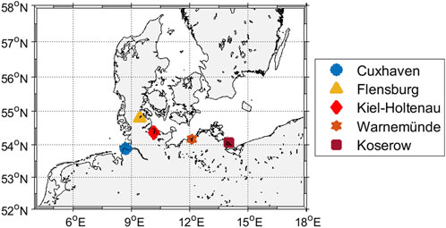
Figure 1. Locations of the investigated gauge stations at the German North- and Baltic Sea coast.

2.1.2 Atmospheric reanalysis data

For the analysis of past meteorological conditions associated with the observed storm surges, we use both the NCEP/NCAR R1 and the ERA5 reanalyses sea level pressure (SLP) data.

The National Centers for Environmental Prediction (NCEP) and the National Center for Atmospheric Research (NCAR) produced the Reanalysis 1 (Kalnay et al., 1996) in close cooperation. The central module is identical to the operational system then used at the NCEP, but with a spectral T62 horizontal resolution, i.e., about 210 km grid spacing and 28 vertical levels. The reanalysis was initially completed in 1996, but continued through an identical Climate Data Assimilation System (CDAS) to ensure consistency with the earlier decades.

ERA5 is one of the most recent reanalysis datasets produced by the European Centre for Medium-Range Weather Forecasts (ECMWF, Hersbach et al., 2020). As such, it is one of the most modern and advanced global reanalyses, using the Integrated Forecasting System (IFS) jointly developed and maintained by ECMWF and Météo-France. The ERA5 data are available on a high-resolution grid with a spacing of 0.25° and in hourly resolution for the period from 1979 to the present and are updated at regular intervals. To additionally cover the period before 1978 we included the ERA5 backward extension (Bell et al., 2021). For this investigation we calculated daily means of the hourly SLP values from 0UTC to 23UTC. The daily SLP means are used to calculate daily weather type classifications, Gale strengths and effective winds.

2.1.3 Climate model simulations

In order to analyse the potential future change of meteorological conditions favorable for storm surges at the German coasts, we make use of an ensemble of global climate models. All simulations of a given experiment are subject to identical external forcings, such as greenhouse gases and aero-sols, following the protocol for the historical experiment of the Coupled Model Intercomparison Project in its sixth phase (CMIP6) (Eyring et al., 2016), and ScenarioMIP (O’Neill et al., 2016), respectively. For the analyses presented in this study, we examined the four Tier1-scenarios of ScenarioMIP that is SSP1-2.6, SSP2-4.5, SSP3-7.0, and SSP5-8.5. The SSP (Shared Socioeconomic Pathways) scenarios span a wide range of socio-economic narratives and greenhouse gas concentration pathways for the remainder of the 21st century (Riahi et al., 2017).

The large number of simulations available for CMIP6 makes it an excellent tool to derive robust estimates of climate change signals projected by these models. Our analyses were based on daily mean SLP fields taken from these simulations. In order to be able to compare our results with a different method that has recently been successfully tested for past storm surges at Cuxhaven (Schaffer et al., 2024), we use only models with a high temporal resolution for the wind components in our ensemble. Altogether, our ensemble consists of seven different GCMs and in total 23 model runs (Table 1).

Table 1

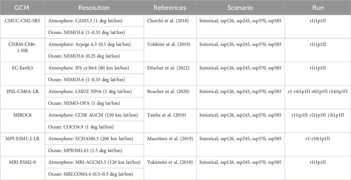
Table 1. Global climate models (GCMs) used for this investigation, including the resolution of the model components for the atmosphere und the ocean, references, scenarios and the respective runs.

2.2 Methods

2.2.1 Defining storm surges

For the German North Sea coast, storm surges are defined as EWLs exceeding 1.5 m above the mean high water (Bundesamt für Seeschifffahrt, 2025). 272 storm tides and respective peak water levels were recorded at the gauge Cuxhaven in the period 1951–2022, which corresponds to an average of about four storm tides per year. It should be emphasized here that these events are not necessarily independent of each other. A large-scale synoptic weather situation may lead to a succession of several high waters that meet the criterion of a storm surge given here. In the following, we detect and treat each storm tide as a separate event ignoring their possible dependence.

For the German Baltic Sea coast, storm surges are defined as EWLs exceeding 1 m above the mean water level (MWL). 184 storm tides were recorded at the gauge Flensburg, 161 at the gauge Kiel-Holtenau, 103 at the gauge Warnemünde, and 105 at the gauge Koserow.

2.2.2 Classification of the large-scale atmospheric circulation

A coherent description of the large-scale atmospheric circulation is possible using defined circulation patterns or weather types (e.g., Lamb, 1950). At BSH, the automatic classification method developed by Jenkinson and Collison (Jenkinson and Collison, 1977) to objectify the “Lamb Weather Types” (hereafter LWTs) is used operationally as part of the analysis of the state of the North Sea region (Löwe, 2005), and, since 2020, for the Baltic Sea region as well. This classification method is also applied in this study. It is solely based on daily means of the SLP fields at 16 grid points $p_x(withx=1\dots 16$) in the extended North or Baltic Seas region (see Figure 2) to calculate the vector components (u*,v*) of the geostrophic wind (V*) and the vorticity (${\mathrm{\zeta }}^{*}$) as described by Löwe (2005), appendix A, GL. A5 - A7 & GL. A13/14), where

$V^{*}\left(hPa\right)=\sqrt{{u^{*}}^2+{v^{*}}^2}$

with

$u^{*}\left(hPa\right)=\frac{1}{2}\left(p_{12}+p_{13}\right)-\frac{1}{2}\left(p_4+p_5\right)$

$v^{*}\left(hPa\right)=\frac{1}{\mathit{cos}{\phi }_0}\left\{\frac{1}{4}\left(p_5+2p_9+p_{13}\right)-\frac{1}{4}\left(p_4+2p_8+p_{12}\right)\right\}$

Figure 2

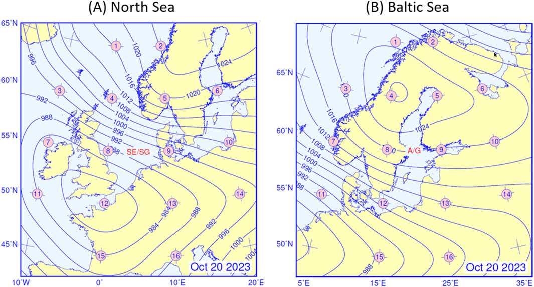
Figure 2. Pressure fields for Oktober 20th, 2023 (storm Babet, UK Met Office) with LWT and Gale Index (red letters) from daily mean of NCEP/NCAR1 sea level pressure in [hPa](blue isolines) over the (A) North and (B) Baltic Seas. Also indicated are the 16 grid points (pink numbered) used to calculate LWTs, Gale index, and the effective geostrophic wind (not pictured here).

And

${\zeta }^{*}\left(hPa\right)={\zeta }_u^{*}+{\zeta }_v^{*}$

with

${\zeta }_u^{*}\left(hPa\right)=\frac{\mathit{sin}{\phi }_0}{\sin \left({\phi }_0+\Delta \phi /2\right)}\left\{\frac{1}{2}\left[\left(p_{15}+p_{16}\right)-\left(p_8+p_9\right)\right]\right\}-\frac{\mathit{sin}{\phi }_0}{\sin \left({\phi }_0-\Delta \phi /2\right)}\left\{\frac{1}{2}\left[\left(p_8+p_9\right)-\left(p_1+p_2\right)\right]\right\}$

${\zeta }_v^{*}\left(hPa\right)=\frac{1}{2{\mathit{cos}}^2{\phi }_0}\left\{\frac{1}{4}\left[\left(p_6+{2p}_{10}+p_{14}\right)-\left(p_5+2p_9+p_{13}\right)\right]-\frac{1}{4}\left[\left(p_4+{2p}_8+p_{12}\right)-\left(p_3+2p_7+p_{11}\right)\right]\right\}$

where ${\phi }_0$ is the latitude of the respective central point of the respective grid (55°N, 5°E for the North Sea; 60°N, 20°E for the Baltic Sea), and $\Delta \phi$ is 10°. The Baltic Sea grid has been shifted 5° north- and 15° eastwards from the North Sea grid to accommodate for the Coriolis frequency, i.e., to ensure that gales are identified at an identical geostrophic wind and vorticity scale in either region.

The geostrophic wind is a good approximation of the large-scale wind conditions in the free atmosphere. The LWTs are derived from the relationships between the geostrophic wind components and the vorticity. While the classification procedure originally allowed for 27 different weather types, a condensed version is used here that identifies six characteristic weather types in order to assure more reliable and robust statistics. This is achieved by reclassifying the hybrid weather types which appear only five to six times a year, and by evenly distributing the rather undistinctive types into two rotational and four directional types (Löwe, 2009; Löwe et al., 2013). These six characteristic weather types are anticyclonic (A), cyclonic (C), north-east (NE), north-west (NW), south-east (SE), and south-west (SW). Although technically only valid at its respective central points, the results are representative of the North- and Baltic Seas.

LWT A is an anticyclone centered over the area with its core at or near the central point and is characterized by mainly dry conditions and light winds, warm in the summer season and cold in winter due to the influence of the continental land masses. LWT C in contrast is a cyclone or depression centered over the area, usually wet with variable wind conditions, mild temperatures in autumn and winter and colder temperatures in spring and summer, oftentimes accompanied by gales or thunderstorms.

The directional LWTs (NE, SE, SW, NW) are defined due to the quadrant, i.e., the directional boundaries of a four-point compass (0°, 90°, 180°, 270°). The classification criteria are summarized in Table 2. LWT SW is characterized by low pressure systems traveling the Atlantic eastwards with mild temperatures, rainfall and frequent gales during the winter months and cool conditions in summer. LWT NW is accompanied by cooler conditions than SW but shows similar overall conditions with low-pressure systems traveling eastwards from Island into the North Sea with greatest intensity over the Baltic or Scandinavia and gale strength winds (Lamb, 1950). Westerly winds would also push water masses onshore the German North Sea Coast and offshore the coast of Schleswig-Holstein, where Kiel and Flensburg are located. LWT NE brings cold arctic air to the area, resulting e.g., in severe frost in winter and water pushed onshore the German Baltic Sea Coast. LWT SE is the main driver for negative storm surges in the German Bight of the North Sea and is characterized by a positive pressure anomaly over Scandinavia and a negative pressure anomaly over the north Atlantic and the Iberian Peninsula (Jensen et al., 2022).

Table 2

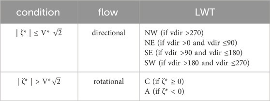
Table 2. Reduced LAMB Weather Type classification criteria based on geostrophic wind (V*), vorticity (${\mathrm{\zeta }}^{*}$) and geostrophic wind direction (vdir).

2.2.3 Gale strength

Another variable that is relevant for storm surges and provided by the LWT classification is the gale strength. A gale index G* is calculated, based on an elliptical relationship between geostrophic wind (V*) and vorticity (${\mathrm{\zeta }}^{*}$) (Löwe, 2005, appendix A3, GL. A16):

$G^{*}=\sqrt{{V^{*}}^2+\frac{{{\mathrm{\zeta }}^{*}}^2}{4}}$

As part of the classification, the gale index is then classified as G (“Gale”), SG (“Severe Gale”) and VSG (“Very Severe Gale”) if it exceeds the 90th, 98th and 99.73rd percentile of the climatological G* distribution based on a reference period of 1971–2000 (Löwe, 2009; Löwe et al., 2013). All values below the 90th percentile are associated with NUL (“No Gale”). Both, daily LWTs and gale strengths data for the North and Baltic Seas from 1948 till 2024 are referenced via the World Data Center for Climate (WDCC), hosted and maintained by the German Climate Computing Center (DKRZ) in Hamburg, Germany (see Loewe, 2022; Loewe and Schade, 2024).

In the specific case depicted in Figure 2, a severe storm surge (storm “Babet”, UK Met Office) was observed on 20 October 2023, along the German and Danish Baltic Sea coast, caused by easterly winds (LWT = A, Gale = G), as well as a negative storm surge (e.g., Jensen et al., 2022) at the North Sea Coast (LWT = SE, Severe Gale = SG). This event was described in several publications (e.g., Groll et al., 2024; Kiesel et al., 2024) and led to substantial damages like dyke breaks and flooding in several cities, e.g., Flensburg and Schleswig at the Baltic Sea coast of Schleswig-Holstein, Germany.

2.2.4 Effective wind

The combination of large-scale wind direction, as indicated by the LWT, and gale strength can be captured by the effective wind. The effective wind is defined as the wind component (or the part of the wind vector) that has the strongest effect on the water level at a specific location. In the cases examined here, this is the wind direction driving the water directly to the gauge station resulting in a storm surge.

In order to identify the wind direction for the effective wind at each station, the respective mean geostrophic wind direction has been calculated by averaging the geostrophic wind components at the respective calendar days of the observed storm surges. In case the peak water levels occurred before 6 a.m., the geostrophic wind components of the previous day were used in order to link the delayed response of the water body to the influence of the wind conditions. Then, the daily geostrophic wind vectors for the entire study period were projected onto the wind direction to calculate the absolute effective wind (v_eff), combining both wind direction and strength into a scalar metric for simplified analysis. Note that the effective wind calculated here is specific to storm surges at the respective gauge stations and the observational time period. This approach has been employed in several studies on storm surges - or their opposite, “negative storm surges” - (e.g., Ganske et al., 2018; Jensen et al., 2022; Koziar et al., 2006) and it has been proven to be effective.

3 Results

The data catalogues of observed peak water levels (see Section 2.1.1) allow a statistical analysis of the common atmospheric conditions at the time of storm surges. The Lamb classification method is employed as described in Section 2.2 to investigate the LWTs, gale indices and effective winds at the respective calendar days of observed storm surges. To account for the influence of the wind conditions on the respective events, all peak water levels occurring before 6 a.m. are linked to the atmospheric conditions the previous day.

3.1 North sea (gauge cuxhaven)

3.1.1 Observed storm surge events

Figure 3A shows the distribution of LWT occurrences at Cuxhaven in the German Bight, calculated from daily NCEP/NCAR R1 SLP data for the entire period (1951–2022), while Figure 3B shows the distribution of LWT occurrences specifically for observed storm surges. The two distributions differ noticeably. During storm surges, the occurrence of LTW NW is threefold higher than in the climatological mean, 61% in total. 14.9% of observed storm surges are associated with LWT SW, and the remaining 24.1% with LWT C, which indicates that the center of the storm is located directly over the central North Sea. Easterly LWTs (SE, NE) are completely missing during storm surges, as well as the LWT A, which could be expected, since westerly winds (especially NW) are needed to push water masses in the direction of the German Bight. Furthermore, the sequence of LWTs SW, C and NW is connected with low pressure systems in this region.

Figure 3

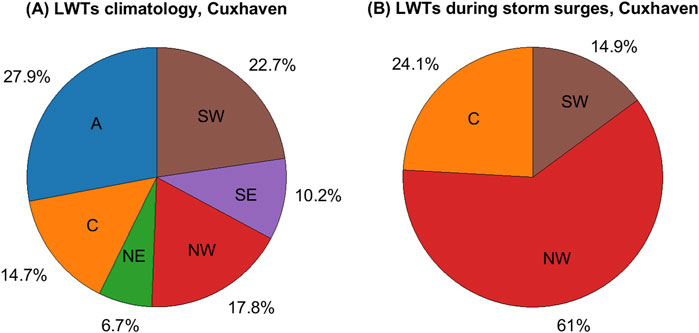
Figure 3. Mean distribution of LWTs determined from daily means of NCEP/NCAR R1 sea level pressure (SLP) for the entire period from 1951 to 2022 (A) and during observed storm surges at the gauge Cuxhaven between 1951 and 2022 (B) Adapted from Schade et al. (2023), Figure 4-1.

Similarly, to Figures 3, 4 shows the distribution of the gale index (G*) derived from the LWT classification. While the probability that a storm (indices G, SG and VSG) occurs is about 9% for all peak water levels, this probability rises to about 84.4% during observed storm surges. The remaining 15.6% show G*-values below the 90th percentile, which were therefore classified as no storm. This is the case for 44 storm surge events from the catalogue. In some of those 44 cases, a storm was detected the day before, or the EWL was caused by a combination of untimely tidal high waters and westerly winds not reaching gale strength. In fact, all those 44 EWL cases show persistent westerly conditions in the days and even weeks before the peak high water, and/or high effective geostrophic wind speeds. Therefore, it proves necessary to analyze the directional component together with its strength. Also, at least part of the 44 EWLs classified with “no gale” could be explained by the presence of external surges (Böhme et al., 2023).

Figure 4

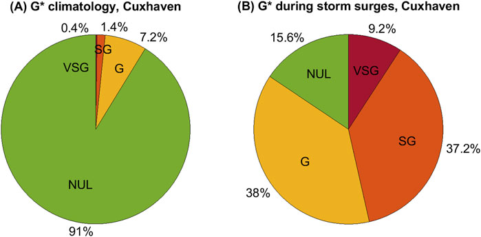
Figure 4. Mean distribution of the gale index (G*) determined from daily means of NCEP/NCAR R1 sea level pressure (SLP) for the entire period from 1951 to 2022 (A) and during observed storm surges at the gauge Cuxhaven between 1951 and 2022 (B). Adapted from Schade et al. (2023), Figure 4-2.

For Cuxhaven, the effective wind direction is 295° (Müller-Navarra and Giese, 1999). Figure 5 shows the empirical probability distribution function of the effective wind (Section 2.2.2) as a climatology for the entire period 1951–2022 and during storm surges in [m/s] using the equations from Löwe (2005); appendix A1, GL. A3/A4). The two distributions are clearly different. During storm surges, the effective wind is always positive and mostly higher than 13 m/s which in turn approx. Matches the 95th percentile of the climatological distribution that is close to the modal value of 14 m/s. The climatological probability distribution of the effective wind spreads from about −23 m/s to 31 m/s with a mean value of approx. 2.4 m/s, indicating a predominant westerly circulation over the North Sea. It is noticeable that a number of storm surges can be observed at v_eff values clearly below the extremes of the climatological distribution. This is in sync with below extreme gale values during observed storm surges and shows that the combined effect of a tidal high-water situation and not extreme westerly winds can lead to extreme peak water levels as well. Further, external surges can contribute to the generation of extreme events under non-extreme wind conditions. Nevertheless, the analysis indicates that v_eff can be used as a proxy to indicate storm surge favorable atmospheric conditions and the 95th percentile of the climatological v_eff distribution can serve as a threshold to identify these situations in climate model simulations.

Figure 5

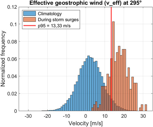
Figure 5. Normalized effective wind (v_eff) distribution determined from daily means of NCEP/NCAR R1 sea level pressure (SLP) and projected onto 295° for the entire period from 1951 to 2022 (blue), and during observed storm surges (orange) at the gauge Cuxhaven between 1951 and 2022. The red line marks the 95th percentile of the climatological distribution. Adapted from Schade et al. (2023), Figure 4-3.

3.1.2 Climate change signals using a CMIP6 ensemble

The results from the previous sections demonstrate that both, wind direction and wind speed play a crucial role in triggering storm surges. The question arises whether these conditions might change in the future. In the following we analyze the frequency of westerly LWTs (SW, NW), including LWT C, gale classes, as well as v_eff in four SSP climate scenarios based on the CMIP6 ensemble (Section 2.1.3).

Figure 6A shows the occurrence of the sum of the derived LWTs NW, C, and SW per year for NCEP/NCAR R1, ERA5 and the 23-member CMIP6 ensemble for the historical period (1971–2000) and the far future (2071–2,100) in SSP1-2.6, SSP2-4.5, SSP3-7.0, and SSP5-8.5, respectively. In these plots, two median values are significantly different (p < 0.05) if their confidence intervals (marked by the center of the triangular markers) do not overlap. It can be concluded that the median occurrences of NW, C and SW LWTs in CMIP6 historical is consistent with those in ERA5, while the occurrences of those LWTs calculated from NCEP is lower.

Figure 6

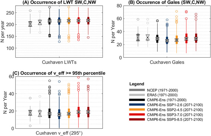
Figure 6. Boxplot of the occurrence of (A) the Lamb Weather Types (LWTs) SW, C, and NW, (B) Gales, and (C) effective geostrophic winds ≥95th percentile at the gauge Cuxhaven (North Sea) for NCEP/NCAR R1 (dark grey), ERA5 (light grey) and the CMIP6 ensemble (black) for the historical period (1971–2000) as well as the respective runs for each the SSP-Scenarios 1–2.6 (blue), 2–4.5 (orange), 3–7.0 (light red), and 5–8.5 (dark red) for the far future (2071–2,100). Boxplots display the median (black dot), the interquartile range (25–27th Percentile, box), the extremes, i.e., approximately ±2.7 sigma and 99.3 coverage, of the distribution (whiskers), and outliers (circles). Notches, depicted as triangles around the median, correspond to q2 - 1.57 (q3 - q1)/sqrt (n) and q2 + 1.57 (q3 - q1)/sqrt (n), where q2 is the median (50th percentile), q1 and q3 are the 25th and 75th percentiles, respectively, and n is the number of observations. Adapted from Schade et al. (2023), Figure 5-1.

The frequency of relevant LWTs hardly changes with the projected climate change according to the CMIP6 data. In the supplements (Supplementary Figure S1) we show the changes in the frequency for all six LWTs. Here we find that LWT C will occur significantly less in a changing climate. The drop is more pronounced in the higher emission scenario. In contrast, both westerly LWTs (NW,SW) show significant increases. This is arguably due to the projected poleward shift of the storm tracks and the cores of the single storm systems, resulting in a more directly westerly driven circulation and therefore a higher probability in the occurrence of v_eff above the 95th percentile (see Figure 6C).

Figure 6B shows the distribution of the occurrence of gales (G, SG, and VSG) during LWTs SW, C, and NW per year for the historical period and the far future. A significant decrease for the SSP1-2.6 scenario is apparent, while the higher scenarios reach historical levels, but with an extended range regarding the extremes.

Figure 6C shows the distribution of the occurrence of effective winds being above the 95th percentile of the climatological probability distribution function of the historical period. For NCEP, this 95th percentile approximately matches the value of 13 m/s, and we have seen in Figure 5 that the majority of storm surges were caused by effective winds beyond this threshold. Hence, we consider such extreme effective winds a reasonable proxy for the risk of storm surges, without including the actual tide phases (or sea level rise for that matter). CMIP6 shows a shift towards more frequent situations with extreme effective winds under the SSP3-7.0, and SSP5-8.5 scenarios. These scenarios have a significantly higher median than in the historical scenario (see also Supplementary Figure S2). This shift can be explained with the significant increase of westerly LWTs, even though the mean frequency of gales during relevant LWT-situations does not change.

3.2 Baltic Sea

3.2.1 Observed storm surge events

Figure 7 shows the frequency distribution of LWTs for observed storm surges at the Baltic Sea gauge stations in Flensburg (A), Kiel-Holtenau (B), Warnemünde (C), and Koserow (D) between 1951 and 2022. Obviously, the situation in the Baltic Sea is completely different from the North Sea. First of all, the storm surge favorable atmospheric conditions are dominated by easterly winds, especially for the more exposed stations at Koserow and Warnemünde (see Figure 1). But even at those stations, storm surges are recorded when the wind comes from westerly directions, i.e., blowing offshore instead of onshore. This is most pronounced for Kiel-Holtenau and Flensburg.

Figure 7

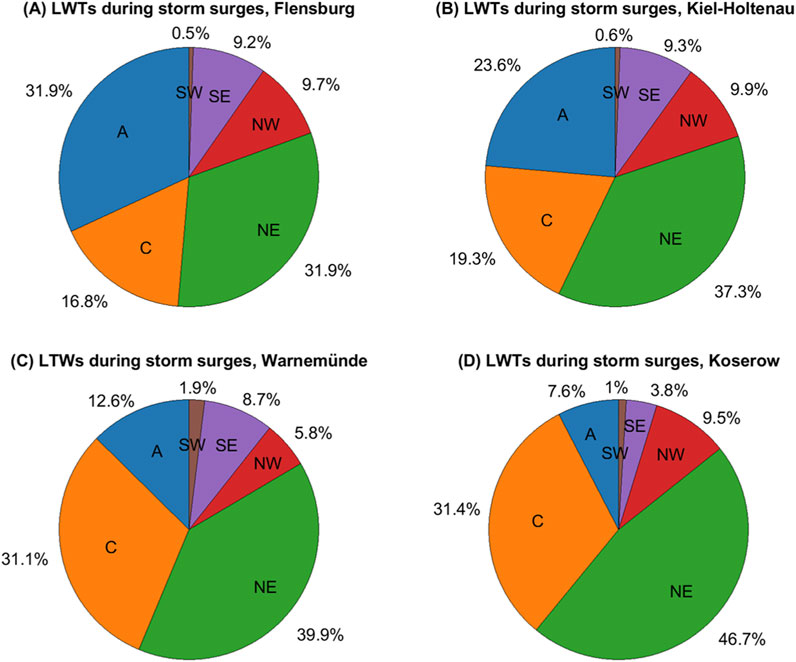
Figure 7. Mean distribution of LWTs determined from daily means of NCEP/NCAR R1 sea level pressure (SLP) during observed storm surges at the gauges Flensburg (A) Kiel-Holtenau (B) Warnemünde (C) and Koserow (D) between 1951 and 2022.

Nevertheless, to obtain a v_eff direction to describe the direct atmospheric trigger for the Baltic Sea gauge stations, the mean v_eff has been derived from the distribution during observed storm surges, exemplary shown as wind roses for four Baltic Sea stations (Figure 8). For Koserow (D), the mean v_eff direction is 34°. Compared to the other Baltic Sea stations, the wind rose is narrower around the mean v_eff direction due to its more exposed location, but still shows some westerly winds during storm surge events. Kiel-Holtenau (B), and Flensburg (A), especially, show a wide spread in directions from north-west to south-east, yet, most directions are north-easterly during storm surges. Therefore, the mean v_eff direction seems mostly feasible to assess the direct atmospheric circulation influence and changes thereof in future scenarios.

Figure 8

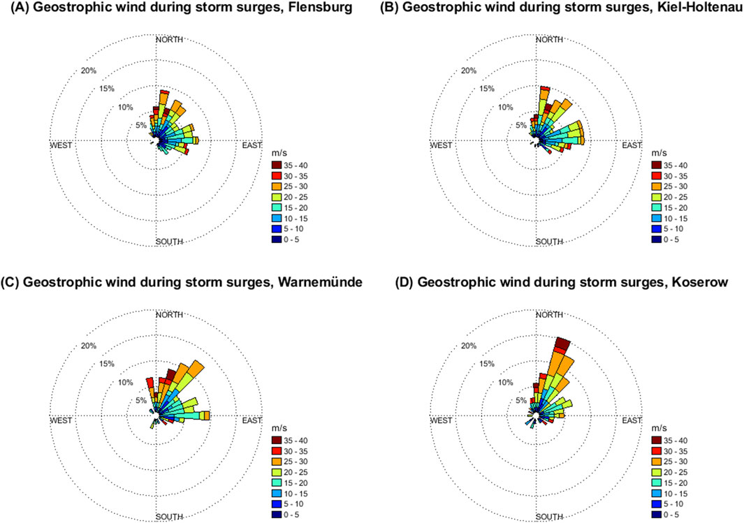
Figure 8. Wind roses from output of LWTs determined from daily means of NCEP/NCAR R1 sea level pressure (SLP) during observed storm surges at gauge stations (A) Flensburg, (B) Kiel-Holtenau, (C) Warnemünde, and (D) Koserow between 1951 and 2022.

Figure 9 shows the empirical probability distribution function of the effective wind speeds for the entire period 1951–2022 and during storm surges for the Baltic Sea stations. As in Cuxhaven, a clear distinction between the two distributions is obvious, but here these differences are not as pronounced. The main difference, however, is that a number of storm surges can be observed at negative v_eff values. This shows again that the atmospheric component is not the sole driver of these extreme peak water level events which becomes even more obvious at the stations Kiel-Holtenau (B) and Flensburg (A) where the 95th percentile is not including the modal value of the geostrophic effective wind speed.

Figure 9

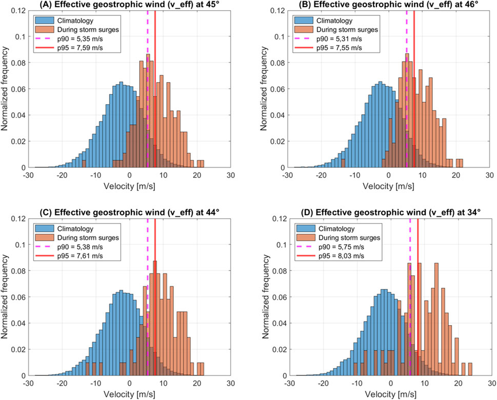
Figure 9. Normalized effective wind (v_eff) distributions determined from daily means of NCEP/NCAR R1 sea level pressure (SLP) for the entire period from 1951 to 2022 (blue), and during observed storm surges (orange) at the gauges (A) Flensburg, (B) Kiel-Holtenau, (C) Warnemünde, and (D) Koserow between 1951 and 2022. The red lines mark the 95th percentiles of the climatological distributions, the dashed magenta lines the 90th percentiles.

However, the analysis indicates that the 95th percentile of the climatological v_eff distribution can serve as threshold to identify storm surge favorable atmospheric conditions in climate model simulations as well. It has to be pointed out here that the 90th percentile could be used instead, especially for the stations Kiel-Holtenau (B) and Flensburg (A), since the modal value of the distribution for actual storm surge events would be included then as well. For consistency reasons, we display the results for the 95th percentile here, but the results using the 90th percentile are included in the supplements. While the total values change of course, the tendencies of the climate change projections do not differ from those using the 95th percentile. We will present the results for Koserow in the following, since the exposed location of the station makes it the best exemplary study case based on the previous results. The results for the other stations will be discussed, but the respective figures are placed in the supplements.

3.2.2 Climate change signals using the CMIP6 ensemble

Figure 10A shows the distribution of the occurrence of the relevant LWTs NE and C per year for NCEP/NCAR R1, ERA5 and the 23-member CMIP6 ensemble for Koserow for the historical period (1971–2000) and the far future (2071–2,100) in SSP1-2.6, SSP2-4.5, SSP3-7.0, and SSP5-8.5, respectively. As for Cuxhaven, the CMIP6 historical ensemble is consistent with ERA5 values regarding the median frequency for the relevant LWTs. The frequency of relevant LWTs hardly changes in the future regardless of the scenario. The same holds true for the other stations (see supplements). Easterly LWTs that favor storm surge conditions in the Baltic occur much less frequent than the corresponding westerly LWTs in Cuxhaven. It should be mentioned that southerly LWTs (SE, SW) are not well represented with the CMIP6 ensemble compared to both reanalyses (Supplementary Figure S3): While SW is significantly underestimated, SE is significantly overestimated. Yet, both LWTs are seldomly associated with storm surges in the Baltic Sea (see Figure 7).

Figure 10

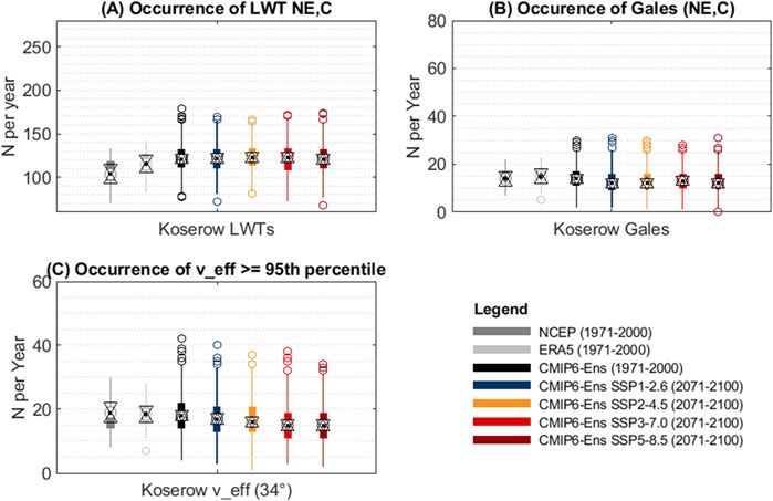
Figure 10. Boxplot of the occurrence of (A) the Lamb Weather Types (LWTs) NE, and C, (B) Gales, and (C) effective geostrophic winds ≥95th percentile at the gauge Koserow (Baltic Sea) for NCEP/NCAR R1 (dark grey), ERA5 (light grey) and the CMIP6 ensemble (black) for the historical period (1971–2000) as well as the respective runs for each the SSP-Scenarios 1–2.6 (blue), 2–4.5 (orange), 3–7.0 (light red), and 5–8.5 (dark red) for the far future (2071–2,100). Boxplots display the median (black dot), the interquartile range (25–27th Percentile, box), the extremes, i.e., approximately ±2.7 sigma and 99.3 coverage, of the distribution (whiskers), and outliers (circles). Notches, depicted as triangles around the median, correspond to q2 - 1.57 (q3 - q1)/sqrt (n) and q2 + 1.57 (q3 - q1)/sqrt (n), where q2 is the median (50th percentile), q1 and q3 are the 25th and 75th percentiles, respectively, and n is the number of observations.

Figure 10B shows the distribution of the occurrence of gales (G, SG, and VSG) during LWTs NE, and C per year for the historical period and the far future. A significant decrease for all the SSP scenarios is apparent, while not as strong for the scenario SSP3-7.0 (see Supplementary Figure S4 for a depiction of changes in the medians and confidence intervals only). An overall decrease can be seen for all scenarios at all the Baltic Seas stations (see Supplementary Figures S5-S7). Compared to gales from westerly directions in the North Sea, easterly gales in the Baltic Sea in general are considerably less frequent as well.

Figure 10C shows the distribution of the occurrence of effective winds being above the 95th percentile of the climatological probability distribution function of the historical period. The CMIP6 data shows a shift towards significant less frequent situations with extreme effective winds under the SSP3-7.0, and SSP5-8.5 scenarios regarding the median frequency. This cannot be explained with the changes of the relevant LWTs NE and C (see Supplementary Figure S3): While there is a decrease of LWT NE for the scenarios SSP3-7.0 and SSP5-8.5, an increase of LWT C for the respective scenarios and SSP2-4.5 can be seen. It is therefore likely explained by the decrease in easterly gales as mentioned above.

Using the 90th percentile of the climatological v_eff distribution as threshold, the results do not change except of course for the overall mean values increasing and, likewise, the amount of decrease in the far future (see Supplementary Figures S8-S11), i.e., the situations with extreme effective winds decrease even more. But one could argue that “extremes” described with values above the 90th percentile of a distribution are not considered statistically extreme values anymore.

4 Discussion

Our investigations of LWTs over the North Sea show that westerly and cyclonic LWTs are the atmospheric drivers at days with observed storm surges at Cuxhaven. For the Baltic Sea region, storm surges can occur with each weather type. Yet, favorable LWTs at the stations Koserow and Warnemünde are NE and C with the addition of A for Kiel and Flensburg.

Towards the end of the 21st century (2071–2,100), the multi-model ensemble projects a significant increase in the frequency of atmospheric conditions favouring storm surges, i.e., westerly effective geostrophic winds, in the direction of Cuxhaven under the scenarios SSP3-7.0 and SSP5-8.5. In contrast, a significant decrease of easterly effective geostrophic winds can be seen in the direction of all four locations at the Baltic Sea coast. These results are in accordance with the projected increased flow from westerly directions and a north-western shift of the storm tracks in climate projections over the North and Baltic Seas region described by other investigations (e.g., Donat et al., 2010; Heinrich et al., 2024; Plavcová and Kyselý, 2013).

Further, our study supports similar investigations that a direct atmospheric trigger is not the sole contributor for the development of EWLs in the German Baltic Sea, and that other factors like the pre-filling due to westerly winds, pushing water masses from the North Sea through the Skagerrak (the strait running between the Jutland peninsula of Denmark, the east coast of Norway, and the west coast of Sweden) or the seiche-effect have to be considered. Groll et al. (2024) for example, showed that two out of the recent three mayor Baltic Sea storm surges were caused by a combination of wind-induced water level and prefilling rather than by extremes in direct atmospheric effects alone. In addition, Lorenz et al. (2024) found that from the three main influences for EWLs (storm surges, seiches, and pre-filling), storm surges dominate the western parts of the Baltic Sea while in the Central and Northern Baltic Sea pre-filling is the main influence (see e.g., their Figure 3). We therefore conclude that EWLs at more exposed stations at the German Baltic Sea coast like Koserow - that are more receptive to a direct wind influence - can be described using our approach while it still works reasonably well for the stations Warnemünde, Kiel-Holtenau and Flensburg.

In the North Sea area, LWTs have been tested as part of the European Cooperation in Science and Technology (COST) Action 733 “Harmonisation and Applications of Weather Type Classifications for European regions” (Philipp et al., 2010), and have proven useful in climate studies (e.g., Fealy and Mills, 2018; Jensen et al., 2022). Recent studies by Krieger and Weisse (2025) using a similar approach namely, calculating geostrophic wind speeds from a triangle of SLP grid points located over the German Bight derived from a slightly enhanced CMIP6 ensemble support our findings of increased (north) westerly winds and a decrease in easterly winds. They also found increases in the very high percentiles (above the 99th), i.e., effective wind speeds above 30 m/s (their Figures 9, 10) in the German Bight. They concluded that the likelihood of very severe storms may increase significantly in a warming climate despite an overall reduction of storm activity. This was also found by Priestley et al., 2020 and is in line with projected storm track changes described by Harvey et al. (2020).

To conclude, we want to highlight that our method can be applied easily to global as well as regional climate model simulations which makes it an effective tool for climate change investigations of the atmospheric conditions that may trigger EWLs. We argue and show that the (large) majority of storm surges are associated with the respective atmospheric circulation patterns. Analysis of the frequency of these weather types therefore yields results that are valuable with respect to potential changes in storm surge risk. Furthermore, a robust assessment of potential climate change signals requires the analysis of multi-model ensembles. These are still only available from GCMs which unfortunately provide only limited output. Therefore, any methods based solely on GCMs without having sub daily information is of particular interest for the community. Further, an advantage of this method is the independence of geostrophic wind speeds on surface wind parametrizations which may differ between models and introduce biases in the analysis of absolute surface or near-surface wind speeds and derived trends (see Krieger and Weisse, 2025). More in depth analyses on storm tracks, however, require a different approach (e.g., Schaffer et al., 2024; Schaffer et al., 2023).

It should be noted here as well that the virtually certain climate change signal of the sea level rise has to be added when assessing the full risk of EWLs along the coastlines in the future. Also, compound events with more than one contributor to add to the EWLs have to be considered. In these cases, the single contributors do not have to be extreme per se, but the combination of two or more contributors may lead to a resulting EWL. This holds especially true for the Baltic Sea, where pre-filling, seiches, sea level rise, and direct atmospheric triggers have to be considered.

Data availability statement

Existing datasets are available from the following publicly accessible sources: 1) Water level observations at Cuxhaven, Kiel-Holtenau, Flensburg, Warnemünde, and Koserow are available from the Federal Waterways and Shipping Administration (WSV). 2) NCEP/NCAR SLP data are operationally used at BSH for calculations of Lamb Weather Types and Gales (see https://www.wdc-climate.de/ui/project?acronym=BSHwt) and are obtained via the NOAA/OAR/ESRL Physical Sciences Laboratory, Boulder, Colorado, USA. (2014). NCEP/NCAR Reanalysis 1: Surface - Sea Level Pressure (Daily), 1948-continuing. https://www.psl.noaa.gov/data/gridded/data.ncep.reanalysis.surface.html. 3) The ERA5-SLP data is publicly available from the Copernicus Climate Change Service (C3S) Climate Data Store (CDS, https://cds.climate.copernicus.eu/datasets). Hersbach, H., Bell, B., Berrisford, P., Biavati, G., Horányi, A., Muñoz Sabater, J., Nicolas, J., Peubey, C., Radu, R., Rozum, I., Schepers, D., Simmons, A., Soci, C., Dee, D., Thépaut, J-N. (2018): ERA5 hourly data on single levels from 1979 to present. Copernicus Climate Change Service (C3S) Climate Data Store (CDS). (accessed on 13 June 2022), DOI: 10.24381/cds.adbb2d47; 4) CMIP6 SLP data: The SLP-fields are publicly available from the from the Earth System Grid Federations (ESGF) for the respective experiments: 5) CMCC-CM2-SR5 (2020): Lovato, Tomas; Peano, Daniele (2020). CMCC CMCC-CM2-SR5 model output prepared for CMIP6 ScenarioMIP. Version 20220627. Earth System Grid Federation. https://doi.org/10.22033/ESGF/CMIP6.1365. 6) CNRM-CM6-1-HR (2019): Voldoire, Aurore (2019). CNRM-CERFACS CNRM-CM6-1-HR model output prepared for CMIP6 ScenarioMIP. Version 20220617. Earth System Grid Federation. https://doi.org/10.22033/ESGF/CMIP6.1388. 7) EC-Earth3 (2019): EC-Earth Consortium (EC-Earth) (2019). EC-Earth-Consortium EC-Earth3 model output prepared for CMIP6 ScenarioMIP. Version 20220603. Earth System Grid Federation. https://doi.org/10.22033/ESGF/CMIP6.251. 8) IPSL-CM6A-LR (2019): Boucher, Olivier; Denvil, Sébastien; Levavasseur, Guillaume; Cozic, Anne; Caubel, Arnaud; Foujols, Marie-Alice; Meurdesoif, Yann; Cadule, Patricia; Devilliers, Marion; Dupont, Eliott; Lurton, Thibaut (2019). IPSL IPSL-CM6A-LR model output prepared for CMIP6 ScenarioMIP. Version 20220603. Earth System Grid Federation. https://doi.org/10.22033/ESGF/CMIP6.1532. 9) MIROC6 (2019): Shiogama, Hideo; Abe, Manabu; Tatebe, Hiroaki (2019). MIROC MIROC6 model output prepared for CMIP6 ScenarioMIP. Version 20220610. Earth System Grid Federation. https://doi.org/10.22033/ESGF/CMIP6.898. 10) MPI-ESM1-2-LR (2019): Wieners, Karl-Hermann; Giorgetta, Marco; Jungclaus, Johann; Reick, Christian; Esch, Monika; Bittner, Matthias; Gayler, Veronika; Haak, Helmuth; de Vrese, Philipp; Raddatz, Thomas; Mauritsen, Thorsten; von Storch, Jin-Song; Behrens, Jörg; Brovkin, Victor; Claussen, Martin; Crueger, Traute; Fast, Irina; Fiedler, Stephanie; Hagemann, Stefan; Hohenegger, Cathy; Jahns, Thomas; Kloster, Silvia; Kinne, Stefan; Lasslop, Gitta; Kornblueh, Luis; Marotzke, Jochem; Matei, Daniela; Meraner, Katharina; Mikolajewicz, Uwe; Modali, Kameswarrao; Müller, Wolfgang; Nabel, Julia; Notz, Dirk; Peters-von Gehlen, Karsten; Pincus, Robert; Pohlmann, Holger; Pongratz, Julia; Rast, Sebastian; Schmidt, Hauke; Schnur, Reiner; Schulzweida, Uwe; Six, Katharina; Stevens, Bjorn; Voigt, Aiko; Roeckner, Erich (2019). MPI-M MPIESM1.2-LR model out-put prepared for CMIP6 ScenarioMIP. Version 20220616. Earth System Grid Federation. https://doi.org/10.22033/ESGF/CMIP6.793. 11) MRI-ESM2-0 (2019): Yukimoto, Seiji; Koshiro, Tsuyoshi; Kawai, Hideaki; Oshima, Naga; Yoshida, Kohei; Urakawa, Shogo; Tsujino, Hiroyuki; Deushi, Makoto; Tanaka, Taichu; Hosaka, Masahiro; Yoshimura, Hiromasa; Shindo, Eiki; Mizuta, Ryo; Ishii, Masayoshi; Obata, Atsushi; Adachi, Yukimasa (2019). MRI MRI-ESM2.0 model output prepared for CMIP6 ScenarioMIP. Version 20220807. Earth System Grid Federation. https://doi.org/10.22033/ESGF/CMIP6.638.

Author contributions

NS: Writing – review and editing, Methodology, Writing – original draft, Conceptualization, Investigation, Visualization, Validation. CJ: Writing – original draft, Investigation, Methodology, Writing – review and editing. TK: Supervision, Conceptualization, Writing – review and editing, Investigation, Writing – original draft.

Funding

The author(s) declare that financial support was received for the research and/or publication of this article. This research is part of the Research Network funded by the German Federal Ministry of Transport (BMV).

Acknowledgments

Baltic Sea peak water levels have been provided by Ines Perlet-Markus and Jürgen Holfort of the German Federal Maritime and Hydrographic Agency (BSH). We acknowledge the World Climate Research Programme (WCRP) for coordinating and promoting CMIP6. We thank the climate modeling groups for producing and making available their model output, the Earth System Grid Federation (ESGF) for archiving the data and providing access, and the multiple funding agencies who support CMIP6 and ESGF. We thank the German Climate Computing Center (DKRZ) for providing their computing resources, as well as Claudia Hinrichs and Laura Schaffer for additional review and proof-reading.

Conflict of interest

The authors declare that the research was conducted in the absence of any commercial or financial relationships that could be construed as a potential conflict of interest.

Generative AI statement

The author(s) declare that no Generative AI was used in the creation of this manuscript.

Publisher’s note

All claims expressed in this article are solely those of the authors and do not necessarily represent those of their affiliated organizations, or those of the publisher, the editors and the reviewers. Any product that may be evaluated in this article, or claim that may be made by its manufacturer, is not guaranteed or endorsed by the publisher.

Supplementary material

The Supplementary Material for this article can be found online at: https://www.frontiersin.org/articles/10.3389/fenvs.2025.1601836/full#supplementary-material

Footnotes

¹https://www.c.de/DE/Services/Messreihen_Dateien_Download/Download_Zeitreihen_node.html.

References

Bell, B., Hersbach, H., Simmons, A., Berrisford, P., Dahlgren, P., Horányi, A., et al. (2021). The ERA5 global reanalysis: preliminary extension to 1950. Quart. J. R. Meteoro Soc. 147, 4186–4227. doi:10.1002/qj.4174

CrossRef Full Text | Google Scholar

Böhme, A., Gerkensmeier, B., Bratz, B., Krautwald, C., Müller, O., Goseberg, N., et al. (2023). Improvements to the detection and analysis of external surges in the north sea. Nat. Hazards Earth Syst. Sci. 23, 1947–1966. doi:10.5194/nhess-23-1947-2023

CrossRef Full Text | Google Scholar

Bott, F., Lohrengel, A.-F., Forbriger, M., Ganske, A., Haller, M., and Herrmann, C. (2020). Klimawirkungsanalyse des Bundesverkehrssystems im Kontext von Stürmen - Schlussbericht des Schwerpunktthemas Sturmgefahren (SP-104) im Themenfeld 1 des BMVI-Expertennetzwerks. doi:10.5675/ExpNBF2020.2020.05

CrossRef Full Text | Google Scholar

Boucher, O., Servonnat, J., Albright, A. L., Aumont, O., Balkanski, Y., Bastrikov, V., et al. (2020). Presentation and evaluation of the IPSL-CM6A-LR climate model. J. Adv. Model Earth Syst. 12, e2019MS002010. doi:10.1029/2019MS002010

CrossRef Full Text | Google Scholar

Brands, S. (2022). A circulation-based performance atlas of the CMIP5 and 6 models for regional climate studies in the northern hemisphere mid-to-high latitudes. Geosci. Model Dev. 15, 1375–1411. doi:10.5194/gmd-15-1375-2022

CrossRef Full Text | Google Scholar

Bundesamt für Seeschifffahrt (2025). Storm surges. Available online at: https://www.bsh.de/EN/TOPICS/Water_levels_and_tides/Storm_surges/Storm_surges_node.html (Accessed June 24, 25).

Google Scholar

Buthe, B., Jakubowski, D. P., and Pütz, T., (2015). BBSR-analysen KOMPAKT 06/2015.

Google Scholar

Cherchi, A., Fogli, P. G., Lovato, T., Peano, D., Iovino, D., Gualdi, S., et al. (2018). Global mean climate and main patterns of variability in the CMCC-CM2 coupled model. J. Adv. Model. Earth Syst. 2018MS001369. 11, 185–209. doi:10.1029/2018MS001369

CrossRef Full Text | Google Scholar

Demuzere, M., Werner, M., van Lipzig, N. P. M., and Roeckner, E. (2009). An analysis of present and future ECHAM5 pressure fields using a classification of circulation patterns. Int. J. Climatol. 29, 1796–1810. doi:10.1002/joc.1821

CrossRef Full Text | Google Scholar

Donat, M., Leckebusch, G., Pinto, J., and Ulbrich, U. (2010). European storminess and associated circulation weather types: future changes deduced from a multi-model ensemble of GCM simulations. Clim. Res. 42, 27–43. doi:10.3354/cr00853

CrossRef Full Text | Google Scholar

Döscher, R., Acosta, M., Alessandri, A., Anthoni, P., Arsouze, T., Bergman, T., et al. (2022). The EC-Earth3 Earth system model for the coupled model intercomparison project 6. Geosci. Model Dev. 15, 2973–3020. doi:10.5194/gmd-15-2973-2022

CrossRef Full Text | Google Scholar

Eyring, V., Bony, S., Meehl, G. A., Senior, C. A., Stevens, B., Stouffer, R. J., et al. (2016). Overview of the coupled model intercomparison project phase 6 (CMIP6) experimental design and organization. Geosci. Model Dev. 9, 1937–1958. doi:10.5194/gmd-9-1937-2016

CrossRef Full Text | Google Scholar

Fealy, R., and Mills, G. (2018). Deriving lamb weather types suited to regional climate studies: a case study on the synoptic origins of precipitation over Ireland. Intl J. Climatol. 38, 3439–3448. doi:10.1002/joc.5495

CrossRef Full Text | Google Scholar

Fernandez-Granja, J. A., Casanueva, A., Bedia, J., and Fernandez, J. (2021). Improved atmospheric circulation over Europe by the new generation of CMIP6 Earth system models. Clim. Dyn. 56, 3527–3540. doi:10.1007/s00382-021-05652-9

CrossRef Full Text | Google Scholar

Ganske, A., Fery, N., Gaslikova, L., Grabemann, I., Weisse, R., and Tinz, B. (2018). Identification of extreme storm surges with high-impact potential along the German north sea coastline. Ocean. Dyn. 68, 1371–1382. doi:10.1007/s10236-018-1190-4

CrossRef Full Text | Google Scholar

Groll, N., Gaslikova, L., and Weisse, R. (2024). Recent Baltic sea storm surge events from A climate perspective (preprint). Sea. Ocean Coast. Hazards. doi:10.5194/egusphere-2024-2664

CrossRef Full Text | Google Scholar

Harvey, B. J., Cook, P., Shaffrey, L. C., and Schiemann, R. (2020). The response of the northern hemisphere storm tracks and jet streams to climate change in the CMIP3, CMIP5, and CMIP6 climate models. J. Geophys. Res. Atmos. 125. doi:10.1029/2020JD032701

CrossRef Full Text | Google Scholar

Heinrich, P., Hagemann, S., and Weisse, R. (2024). Automated classification of atmospheric circulation types for compound flood risk assessment: CMIP6 model analysis utilising a deep learning ensemble (preprint). Review. doi:10.21203/rs.3.rs-4017900/v1

CrossRef Full Text | Google Scholar

Herrera-Lormendez, P., Mastrantonas, N., Douville, H., Hoy, A., and Matschullat, J. (2022). Synoptic circulation changes over central Europe from 1900 to 2100: reanalyses and coupled model intercomparison project phase 6. Intl J. Climatol. 42, 4062–4077. doi:10.1002/joc.7481

CrossRef Full Text | Google Scholar

Hersbach, H., Bell, B., Berrisford, P., Hirahara, S., Horányi, A., Muñoz-Sabater, J., et al. (2020). The ERA5 global reanalysis. Q.J.R. Meteorol. Soc. 146, 1999–2049. doi:10.1002/qj.3803

CrossRef Full Text | Google Scholar

Hess, P., and Brezowsky, H. (1952). Katalog der Großwetterlagen Europas (No. 33), Berichte des Deutschen Wetterdienstes. Deutscher Wetterdienst. Available online at: https://dwdbib.dwd.de/retrosammlung/content/titleinfo/4180.

Google Scholar

Jenkinson, A., and Collison, F. (1977). An initial climatology of gales over the north sea. Synop. Climatol. branch Memo. 62, 18.

Google Scholar

Jensen, C., Mahavadi, T., Schade, N. H., Hache, I., and Kruschke, T. (2022). Negative storm surges in the elbe Estuary—large-scale meteorological conditions and future climate change. Atmosphere 13, 1634. doi:10.3390/atmos13101634

CrossRef Full Text | Google Scholar

Kalnay, E., Kanamitsu, M., Kistler, R., Collins, W., Deaven, D., Gandin, L., et al. (1996). The NCEP/NCAR 40-Year reanalysis project. Bull. Am. Meteorological Soc. 77, 437–471. doi:10.1175/1520-0477(1996)077<0437:TNYRP>2.0.CO;2

CrossRef Full Text | Google Scholar

Kew, S. F., Selten, F. M., Lenderink, G., and Hazeleger, W. (2013). The simultaneous occurrence of surge and discharge extremes for the rhine Delta. Nat. Hazards Earth Syst. Sci. 13, 2017–2029. doi:10.5194/nhess-13-2017-2013

CrossRef Full Text | Google Scholar

Kiesel, J., Wolff, C., and Lorenz, M. (2024). Brief communication: from modelling to reality – flood modelling gaps highlighted by a recent severe storm surge event along the German Baltic sea Coast. Nat. Hazards Earth Syst. Sci. 24, 3841–3849. doi:10.5194/nhess-24-3841-2024

CrossRef Full Text | Google Scholar

Koziar, C., Renner, V., and Wetterdienst, D. (2006). KFKI-Projekt: muse. Hamburg: Deutscher Wetterdienst.

Google Scholar

Krieger, D., and Weisse, R. (2025). “CMIP6 multi-model assessment of northeast Atlantic and German bight storm activity (preprint),” in Natural hazards and extreme Events/human/earth system Interactions/earth system and climate modeling. doi:10.5194/egusphere-2025-111

CrossRef Full Text | Google Scholar

Lamb, H. H. (1950). Types and spells of weather around the year in the British isles: annual trends, seasonal structure of the year, singularities. Q. J. R. Meteorological Soc. 76, 393–429. doi:10.1002/qj.49707633005

CrossRef Full Text | Google Scholar

Loewe, P. (2022). Lamb weather types (reduced set) and gale days over the north sea since 1948 based on NCEP/NCAR reanalysis 1 daily mean sea level pressure fields. doi:10.26050/WDCC/LambWTyRSetAndGaleDaysOverTheNo

CrossRef Full Text | Google Scholar

Loewe, P., and Schade, N. (2024). Lamb weather types (reduced set) and gale days over the Baltic sea since 1948 based on NCEP/NCAR reanalysis 1 daily mean sea level pressure fields. doi:10.26050/WDCC/LambWTyRSetAndGaleDaysOverTheBa

CrossRef Full Text | Google Scholar

Lorenz, M., Viigand, K., and Gräwe, U. (2024). Untangling the waves: decomposing extreme sea levels in a non-tidal basin, the Baltic sea (preprint). Sea. Ocean Coast. Hazards. doi:10.5194/nhess-2024-198

CrossRef Full Text | Google Scholar

P. Löwe (2005). Nordseezustand 2003, Berichte des BSH, Nr, 38, 220p. Available online at: https://www.bsh.de/download/Berichte-des-BSH-38.pdf.

Google Scholar

P. Löwe (2009). System Nordsee – Zustand 2005 im Kontext langzeitlicher Entwicklungen, Berichte des BSH, Nr. 44, Bundesamt für Seeschifffahrt und Hydrographie, Hamburg und Rostock. Available online at: https://www.bsh.de/download/Berichte-des-BSH-44.pdf.

Google Scholar

P. Löwe, H. Klein, and S. Weigelt-Krenz (2013). System Nordsee – 2006 & 2007: Zustand und Entwicklungen, Berichte des BSH, Nr. 49, Bundesamt für Seeschifffahrt und Hydrographie, Hamburg und Rostock. Available online at: https://www.bsh.de/download/Berichte-des-BSH-49.pdf.

Google Scholar

Mauritsen, T., Bader, J., Becker, T., Behrens, J., Bittner, M., Brokopf, R., et al. (2019). Developments in the MPI-M Earth system model version 1.2 (MPI-ESM1.2) and its response to increasing CO ₂. J. Adv. Model. Earth Syst. 11, 998–1038. doi:10.1029/2018MS001400

PubMed Abstract | CrossRef Full Text | Google Scholar

Meyer, E. M. I., and Gaslikova, L. (2024). Investigation of historical severe storms and storm tides in the German bight with century reanalysis data. Nat. Hazards Earth Syst. Sci. 24, 481–499. doi:10.5194/nhess-24-481-2024

CrossRef Full Text | Google Scholar

Müller-Navarra, S. H., and Giese, H. (1999). Improvements of an empirical model to forecast wind surge in the German bight. Dtsch. Hydrogr. Z. 51, 385–405. doi:10.1007/BF02764162

CrossRef Full Text | Google Scholar

O’Neill, B. C., Tebaldi, C., van Vuuren, D. P., Eyring, V., Friedlingstein, P., Hurtt, G., et al. (2016). The scenario model intercomparison project (ScenarioMIP) for CMIP6. Geosci. Model Dev. 9, 3461–3482. doi:10.5194/gmd-9-3461-2016

CrossRef Full Text | Google Scholar

Philipp, A., Bartholy, J., Beck, C., Erpicum, M., Esteban, P., Fettweis, X., et al. (2010). Cost733cat – a database of weather and circulation type classifications. Phys. Chem. Earth, Parts A/B/C 35, 360–373. doi:10.1016/j.pce.2009.12.010

CrossRef Full Text | Google Scholar

Plavcová, E., and Kyselý, J. (2013). Projected evolution of circulation types and their temperatures over central Europe in climate models. Theor. Appl. Climatol. 114, 625–634. doi:10.1007/s00704-013-0874-4

CrossRef Full Text | Google Scholar

Priestley, M. D. K., Ackerley, D., Catto, J. L., Hodges, K. I., McDonald, R. E., and Lee, R. W. (2020). An overview of the extratropical storm tracks in CMIP6 historical simulations. J. Clim. 33, 6315–6343. doi:10.1175/JCLI-D-19-0928.1

CrossRef Full Text | Google Scholar

Riahi, K., van Vuuren, D.P., Kriegler, E., Edmonds, J., O’Neill, B.C., and Fujimori, S. (2017). The Shared Socioeconomic Pathways and their energy, land use, and greenhouse gas emissions implications: An overview. Global Environmental Change 42, 153–168. doi:10.1016/j.gloenvcha.2016.05.009

CrossRef Full Text | Google Scholar

Riediger, U., and Gratzki, A. (2014). Future weather types and their influence on mean and extreme climate indices for precipitation and temperature in central Europe. metz 23, 231–252. doi:10.1127/0941-2948/2014/0519

CrossRef Full Text | Google Scholar

Schade, N. H. (2017). Evaluating the atmospheric drivers leading to the December 2014 flood in schleswig-holstein, Germany. Earth Syst. Dynam. 8, 405–418. doi:10.5194/esd-8-405-2017

CrossRef Full Text | Google Scholar

Schade, N. H., Jensen, C., Schaffer, L., Ditzinger, G. X., Möller, J., and Kruschke, T. (2023). Wirkungsanalyse Sturm/Sturmfluten, Sonderanalysen und methodische Entwicklungen Berichtsreihe des Schwerpunktthemas 101. Bundesamt für Seeschifffahrt Hydrogr. (BSH). doi:10.57802/44q8-4h46

CrossRef Full Text | Google Scholar

Schade, N. H., Sadikni, R., Jahnke-Bornemann, A., Hinrichs, I., Gates, L., Tinz, B., et al. (2018). The KLIWAS north sea climatology. Part II: assessment against global reanalyses. J. Atmos. Ocean. Technol. 35, 127–145. doi:10.1175/JTECH-D-17-0045.1

CrossRef Full Text | Google Scholar

Schaffer, L., Becker, N., Schenk, L., Hinrichs, C., Ditzinger, G., Schade, N. H., et al. (2023). Objective assessment of storm surge risk in the German bight – historical events and future climate change (other). oral. doi:10.5194/egusphere-egu23-7236

CrossRef Full Text | Google Scholar

Schaffer, L., Boesch, A., Baehr, J., and Kruschke, T. (2024). Development of a wind-based storm surge model for the German bight (preprint). Sea. Ocean Coast. Hazards. doi:10.5194/egusphere-2024-3144

CrossRef Full Text | Google Scholar

Stryhal, J., and Huth, R. (2019). Trends in winter circulation over the British isles and central Europe in twenty-first century projections by 25 CMIP5 GCMs. Clim. Dyn. 52, 1063–1075. doi:10.1007/s00382-018-4178-3

CrossRef Full Text | Google Scholar

Tatebe, H., Ogura, T., Nitta, T., Komuro, Y., Ogochi, K., Takemura, T., et al. (2019). Description and basic evaluation of simulated mean state, internal variability, and climate sensitivity in MIROC6. Geosci. Model Dev. 12, 2727–2765. doi:10.5194/gmd-12-2727-2019

CrossRef Full Text | Google Scholar

Voldoire, A., Saint-Martin, D., Sénési, S., Decharme, B., Alias, A., Chevallier, M., et al. (2019). Evaluation of CMIP6 DECK experiments with CNRM-CM6-1. J. Adv. Model. Earth Syst. 11, 2177–2213. doi:10.1029/2019MS001683

CrossRef Full Text | Google Scholar

Wyser, K., Koenigk, T., Fladrich, U., Fuentes-Franco, R., Karami, M. P., and Kruschke, T. (2021). The SMHI large ensemble (SMHI-LENS) with EC-Earth3.3.1. Model Dev. 14, 4781–4796. doi:10.5194/gmd-14-4781-2021

CrossRef Full Text | Google Scholar

Yukimoto, S., Kawai, H., Koshiro, T., Oshima, N., Yoshida, K., Urakawa, S., et al. (2019). The meteorological research institute Earth system model version 2.0, MRI-ESM2.0: Description and basic evaluation of the physical component. J. Meteorological Soc. Jpn. 97, 931–965. doi:10.2151/jmsj.2019-051

CrossRef Full Text | Google Scholar

Zappa, G., and Shepherd, T. G. (2017). Storylines of atmospheric circulation change for European regional climate impact assessment. J. Clim. 30, 6561–6577. doi:10.1175/JCLI-D-16-0807.1

CrossRef Full Text | Google Scholar