Performance assessment of drone-based photogrammetry coupled with machine-learning for the estimation of hail size distributions on the ground

Hail-producing convective thunderstorms are a major threat to agriculture and infrastructure causing large financial losses. Remote sensing techniques such as dual-polarimetric weather radar can provide hail observations over large areas, but do not necessary reflect the situation on the ground. Current ground-based observations—such as automatic hail sensors, hail pads, and crowd-sourced reports—provide valuable information but exhibit limitations for validating radar products in terms of area coverage. Drone-based hail photogrammetry coupled with machine-learning (ML) techniques has the potential to close this observational gap by sampling thousands of hailstones within the hail core across large areas of hundreds of square meters and provide a hail size distribution estimation. However, the reliability of this new technique has not yet been assessed. In this study, we conducted experiments on different grass surfaces using synthetic hail objects of known sizes and quantity to assess the uncertainty of the ML-based hail size distribution retrievals. The findings of the experiments are then compared with a real hail event surveyed using drone-based hail photogrammetry. Using drone-based hail photogrammetry coupled with ML, 98% of the synthetic hail objects and 81% of hailstones were correctly detected. Additionally, sizes of the detected objects were retrieved with a minor underestimation of around −0.75 mm across all sizes for both synthetic hail objects (10–78 mm) and hailstones (3–24 mm). Hence, the high accuracy coupled with a large sampling area provides an estimation of representative hail size distributions on the ground. These reliable ground observations are a valuable basis for applications such as validation of weather radar hail estimates.

1 Introduction

Hail bears a major threat to society, with single regional events causing economic losses of up to CHF 400 million (Gebäudeversicherung Luzern GVL, 2022). Such a particular extreme event related to a severe convective weather outbreak in Switzerland is described in detail by Kopp et al. (2023b), while event intensity tends to increase in the future across many regions around the globe (Battaglioli et al., 2023; Raupach et al., 2021).

Current hail warning systems rely on a combination of products including satellite imagery, lightning data, numerical weather prediction models, digital elevation models, and importantly, weather radar observations. Weather radar observations enable the detection of hail in thunderstorm cells, along with the prediction of the cell evolution in the next minutes to hours (Germann et al., 2022). An example is the MeteoSwiss thunderstorm radar tracking (TRT) algorithm, operational since the early 2000s (Hering et al., 2004). TRT uses an object detection technique combined with velocity advection schemes to extrapolate storm movements and to identify warning areas. Various algorithms have been developed and are running operationally to identify the probability of hail (POH, Witt et al., 1998; Waldvogel et al., 1979) and the maximum expected severe hail size (MESHS, Treloar, 1998) based on radar signatures (Hering and Betschart, 2012). Additional use of polarimetric signatures of weather radar data enables hydrometeor classification, which could enhance operational hail detection (Besic et al., 2016; Grazioli et al., 2019) and nowcasting (Rombeek et al., 2024) in the future. Nowadays, machine-learning (ML) techniques integrate these data sources to predict storm cell evolution more accurately (Leinonen et al., 2023). However, all these observations only serve as indirect proxies for hail in the atmosphere, and thus extrapolation to predict the impact of hail on the ground involves significant uncertainty (Schuster et al., 2006). Therefore, ground-based observations are essential to verify and improve hail estimations.

Various ground-based observation technologies are widely used to verify and improve these indirect hail estimations. In the late seventies, 330 hail pads were installed in a large-scale field experiment in Switzerland to analyze hail size distributions (HSD) and associated properties, such as kinetic energy (Federer et al., 1986). Hail pads are still commonly used in many field campaigns nowadays thanks to their ease in installation and low cost (e.g., Dessens et al., 2007; Punge and Kunz, 2016; Brimelow et al., 2023). Since 2018, a network of automatic hail sensors is operational in three hail-prone regions in Switzerland. These sensors estimate the size of individual hailstones by measuring the kinetic energy of their impact. The associated datasets have been extensively studied: they have been used to infer the spatio-temporal invariance of normalized hail size distributions and to model them (Ferrone et al., 2024), and they have been compared with hail pad data (Kopp et al., 2023a) and crowd-sourced hail data (Barras et al., 2019). Crowd-sourced hail data is currently the third method operationally used by MeteoSwiss to observe hail on the ground providing information about the size of single hailstones in populated areas (Kopp et al., 2024).

Within the last decade, these three independent and complementary observational methods, namely, hail pads, automatic hail sensors and crowd sourcing, lead to large progress in characterizing the regional distribution of hail. However, observational gaps remain, particularly when hail size distribution is of interest. In fact, weather radar data can provide hail size estimation and information about the probability of hail across large areas, but only via an indirect estimation at a resolution of roughly 1 km². Hail pads have limitations due to their manual data collection process and missing time information. Automatic hail sensors provide precise point observations of HSD, but only across the observational area of 0.2 m². Crowd-sourced data offers extensive spatial coverage but with limited accuracy and observer bias towards populated areas (Barras et al., 2019; Allen and Tippett, 2021).

Photogrammetry is widely used in many fields to map, measure and reconstruct objects of interest from individual images (e.g., Kraus, 2007; Groos et al., 2019; An et al., 2025). In recent years, innovative methods based on aerial photogrammetric data from uncrewed autonomous vehicles (UAVs or drones) for observing hail size distributions have emerged. Images of hail on the ground recorded by a drone were analyzed using a ML method to estimate the HSD (Soderholm et al., 2020; Lainer et al., 2024). Thanks to UAVs, large areas of several hundred square meters can be covered, with corresponding HSDs that can include thousands of individual hailstones. Given that automatic hail sensors record a number of impacts typically in the order of 10–80 per event, the integration of observations from UAVs coupled with ML is expected to complement and improve estimations of HSD.

However, this UAV coupled with ML method involves several challenges. Firstly, in terms of logistics, it is difficult to perform the measurements at the right location and at the right time, as this involves to be physically present within the center of the hail core, shortly after the event, before significant melting occurs. Secondly, the data collection process is time-consuming as it involves preparing the UAV and its flight path, placing reference objects on the ground and flying over the area in a grid-like manner. Another challenge is the assessment of its performance, given the absence of ground truth measurements. The two published events so far rely on size estimations from photogrammetric imagery, supplemented by limited field observations by eye and comparisons with nearby automatic hail sensors (Soderholm et al., 2020; Lainer et al., 2024). However, the true sizes and number of hailstones remain undetermined. Additionally, the UAV cannot be operated in the hail streak itself due to the environmental conditions, such as severe wind gust, hail damaging the UAV, or intense precipitation. Thus, the observations are temporally separated and melting can occur during the time delay between the hail event and the drone flight (usually in the order of 5–10 min). The surface on which the photogrammetric data is collected, which can vary between events, further adds complexity. The most promising surfaces are soccer fields, which can be identified prior and during the storm chase based on map data, and are usually of uniform conditions (short grass without bare soil spots). However, the choice of surfaces is also limited by regulatory restrictions on drone operations. Finally, light conditions during data collection play a critical role. The diurnal cycle of (large) hail usually peaks in the afternoon to evening (Nisi et al., 2020; Hulton and Schultz, 2024) and natural illumination is reduced underneath thunderstorm clouds, impacting the collection of suitable photogrammetric data.

In this study, we conducted an experiment using the approach demonstrated by Soderholm et al. (2020) and Lainer et al. (2024) in order to assess the performance of the drone-based hail photogrammetry method in retrieving HSDs. In the framework of a master thesis (Portmann, 2024), we tested the approach on synthetic hail objects of known number and size on different types of grass. This allowed us to quantify the differences between the HSD of the synthetic objects and the drone-derived HSD.

The current paper is structured as follows. Section 2 presents the equipment used to collect the photogrammetric data, the characterization of the three synthetic hail objects employed to mimic hail properties (expanded polystyrene EPS, glass pebbles, and ice cones), illustrates the various surfaces selected for the experiment, and describes a hail event occurred on 28 June 2022 in Locarno (Switzerland), which serves as a comparison for the experimental results. Section 3 describes the methodology, followed by a presentation of the results in Section 4, showing that around 98% of synthetic hail objects were correctly detected, with a mean bias of around (−0.75$\pm$ 1.6) mm and 81% of hailstones in the real event were correctly detected with a mean bias of around (−0.79 $\pm$ 1.5) mm. In the discussion (Section 5), the results are put into context with data collected from the real hail event in Locarno. Finally, Section 6 presents the conclusions of the study and discusses future research directions.

2 Materials and equipment

In this section, we first present the hardware used to collect the photogrammetric images for the experiments and the real hail event (Section 2.1), followed by a detailed description of the synthetic hail objects used and the grass surfaces selected for the experiments (Section 2.2) and finally, we provide a characterization of the hail event in Locarno (Section 2.3).

2.1 Photogrammetry system

Photogrammetric methods can be used to determine the location, shape and size of objects in measurements retrieved from cameras. This enables the derivation of various products, such as point clouds (PC), geometric models or rectified images (orthophotos) (Kraus, 2007).

Data collection was performed using the commercial multicopter drone DJI Matrice 300 RTK and the DJI Zenmuse P1 camera (DJI, 2020a; 2021). This setup is described in more detail in Lainer et al. (2024). Whilst the hardware is similar, specific settings vary between the synthetic hail experiments, the real hail event presented in Section 2.3, and the hail event presented in Lainer et al. (2024). An overview of the hardware and settings is provided in Table 1.

Table 1

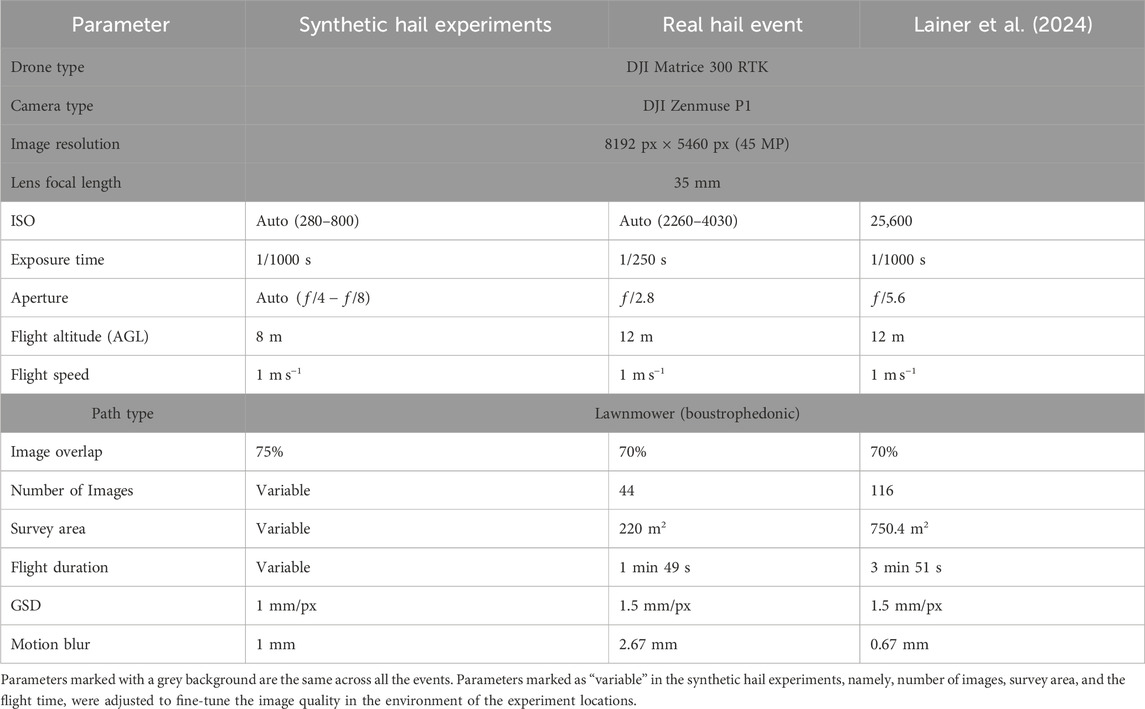
Table 1. Hardware and settings used during the photogrammetric data collection of the cases presented in this paper, synthetic hail experiment and the real hail event that occurred in 2022 in Locarno, with regards to those used in Lainer et al. (2024).

The flight planning software UgCS was used to setup the drone flight paths with the specific parameters (SPH Engineering, 2024). Digital elevation models (DEM) can be loaded, which are available for Switzerland in high resolution (0.5 m) as 1 km² grid cells (Federal Office of Topography swisstopo, 2023), providing detailed surface elevation information. This allows the drone to maintain a constant altitude above ground level (AGL), which is essential for a uniform ground sampling distance (GSD). Photogrammetry parameters can be directly defined in the software. These parameters include the flight patterns, the GSD, the overlap between images, the flight speed and the camera angle. With UgCS, the minimum altitude AGL corresponds to 6 m, while in the DJI Pilot 2 app, as used by Lainer et al. (2024), the minimum flight altitude was restricted to 12 m AGL, resulting in a GSD of 1.5 mm/px (Table 1). The individual photos are taken with a constant exposure time during the flight while the drone is moving, leading to motion blur. The exposure time is set as low as possible and the speed is chosen such that motion blur is below or at the resolution of the GSD. Motion blur $b$ is calculated as:

$b=\frac{v\cdot t_e}{\text{GSD}}$

where $v$ is the flight speed of the drone, $t_e$ the exposure time. For a GSD of 1 mm/px, the motion blur is exactly 1 px at an exposure time of $t_e$ = 1/1000 s. These values were used during the synthetic hail experiments. Due to low light conditions, an exposure time of 1/250 s was used for the real hail event (Table 1). Aperture opening (f-number) and sensor sensitivity (ISO setting) were set to automatic, with metering set to average.

2.2 Synthetic hail experiments

This section introduces the synthetic hail objects used for the experiments (Section 2.2.1), the different surfaces (Section 2.2.2) and the experimental setup (Section 2.2.3).

2.2.1 Synthetic hail objects used for experiments

Commercially available synthetic objects were used to mimic hail in terms of optical properties, size and number distributions. Hereafter, these objects are referred to as “synthetic hail objects” and include EPS spheroids, painted oblate glass pebbles and ice from a consumer-grade ice maker (Figure 1).

Figure 1

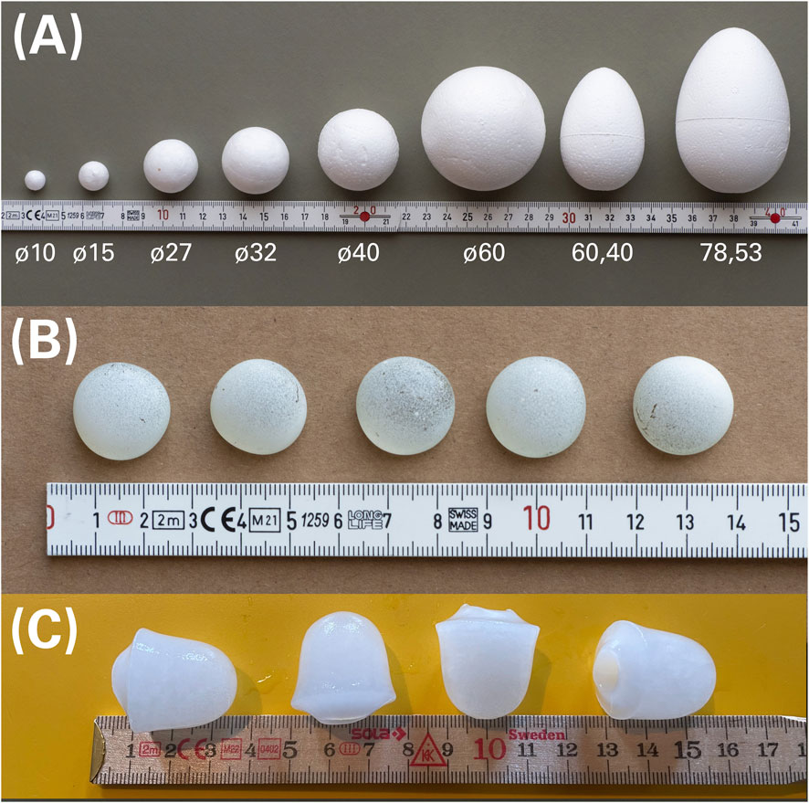
Figure 1. Synthetic hail objects used for the experiments. (A) EPS hail objects (10 mm–78 mm) with their measurements in mm, (B) Oblate, painted glass pebbles (\diameter 19.5 mm), (C) ice hail objects (25 mm$\times$25 mm).

First, EPS hail objects were used to imitate different sizes (major axes from 10–78 mm) and axis ratios (spheres, spheroid ovals) of hail. The size distribution of the EPS spheroids are listed in Table 2, where $d_{\text{ref}}$ is the size reported by the manufacturer, which slightly deviates from the actual size $(d_{\text{act}})$. For the subsequent size estimation, the reference sizes given by the manufacturer are used. The intrinsic limitation of this approach and the uncertainties introduced are discussed in Section 5. In the experimental setup, the EPS hail objects were fixed to the ground with wooden sticks to prevent unintended displacement caused by drone-induced rotor wind or natural wind at the experiment site. In half of the experiments with EPS hail objects, the largest three EPS spheres were substituted by spheroid oval EPS objects to assess the axis ratio of non-spherical objects (see Table 2). In total, 50 EPS hail objects were used in each experiment.

Table 2

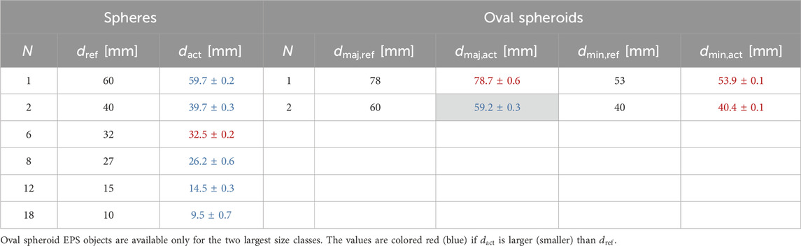
Table 2. Number $(N)$ and size $(d)$ of spherical (diameter) and oval (major and minor axes) EPS objects used per experiment: $d_{\text{ref}}$ refers to the sizes reported by the manufacturer, while $d_{\text{act}}$ indicates the measured mean $\pm$ standard deviation of the actual objects used in this study.

Second, glass pebbles with a flat base and coated with a thin layer of white spray-paint were used to replicate the translucent characteristic of hail, which cannot be represented by EPS hail objects (Figure 1). These glass pebbles are off-the-shelf aquarium decoration of uniform size (19.5 mm $\times$ 19.5 mm $\times$ 0.9 mm) and are thereafter referred to as glass hail objects. During each synthetic hail experiment, 50 glass hail objects were used.

Third, ice produced by an ice maker in cylindrical form were used to emulate hail in terms of albedo, translucency and color (Figure 1). These ice objects have a size of 25 mm $\times$ 25 mm $\times$ 25 mm (measured in the field before placement). They were produced in the evening prior to the experiment and stored in the freezer over night. In the morning, the ice objects were transferred to a thermally isolated container until used in the field experiment. Since the ice objects start to melt when laid out in the field, their size will subsequently be smaller than initially determined. During each synthetic hail experiment, 50 ice hail objects were used.

2.2.2 Experiment surfaces

In order to assess the sensitivity of automatic HSD retrievals as a function of different surfaces, synthetic hail experiments were conducted on various grass surfaces with distinct visual properties. Five sites with varying grass coverage were selected, from dense and uniform soccer fields to patchy meadows, occasionally featuring some flowers such as dandelions or clovers (Figure 2).

Figure 2

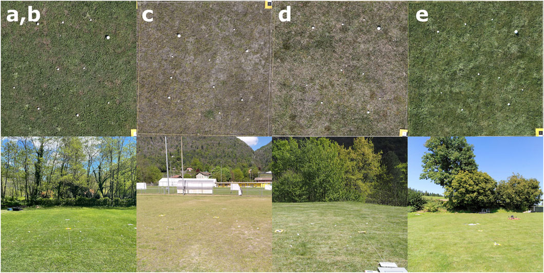
Figure 2. Surfaces of the experiments (a–e). Top row: Excerpts from orthophotos. Bottom row: Images showing the surroundings of the experiment sites. Surfaces (a–d) are soccer fields and e is an airfield for remote-controlled model airplanes. The surfaces can be characterized as follows: (a,b) short, high-density grass of uniform length with small dirt patches, (c) short, very low-density grass of uniform length with large dirt patches, (d) long, medium density grass with high plant variety and no dirt patches, (e) long, very high-density grass of varying lengths with no dirt patches. Due to a different setup (Section 2.2.3), configurations (a,b) share the same type of surface. Experiments on surface (a–d) were conducted during April 2024 in Ticino (southern Switzerland), while experiments on surface e were conducted in August 2024 near Zurich (northern Switzerland).

2.2.3 Experimental setup and dataset

On each surface, an experiment area of 5 m$\times$5 m was defined and divided into four quadrants (Figure 3A). The hail objects (EPS, glass and ice, see Section 2.2.1) were sparsely distributed in two of the quadrants, arranged according to a predefined template to ensure consistent placement across the different surfaces. In one of the quadrants with EPS synthetic hail objects, the largest spheres were replaced by the oval spheroid counterparts with a similar minor axis (diameters 60 mm and 40 mm, Table 2). Ground control points (GCP) with 150 mm side length were placed in the middle and to the side of the experiment area to verify the GSD. One type of synthetic hail objects was placed in the area, and the experiment flight was then completed. This process was repeated for each type of synthetic hail object and on each surface type.

Figure 3

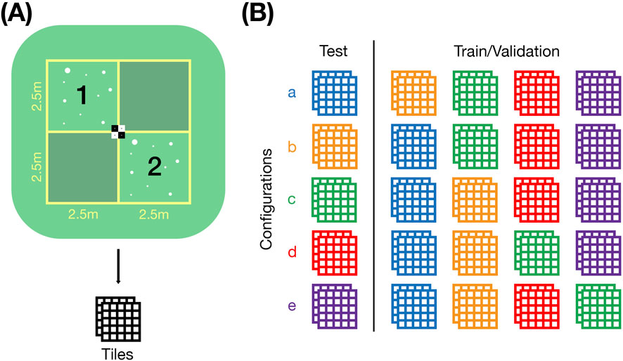
Figure 3. Design of the experiments with synthetic hail objects. (A) Setup of the experiments with the 5 m$\times$5 m square, subdivided into the quadrants and quadrants 1 and 2 are used for this study. Each quadrant is split into 25 tiles of 600 px$\times$600 px, including a 50 px overlap in each direction to prevent cutting off hail objects. (B) All tiles of the two quadrants from each configuration (a–e), are used in a leave-one-out cross-validation (LOOCV) during the ML process. Thus to train the ML model for testing on surface a, all quadrants of the remaining surfaces (b–e) are used as training and validation set and the tiles of the quadrants from surface a is used as the test dataset. This is referred to as configuration (a).

For the training and validation of the ML process, a leave-one-out cross-validation (LOOCV) is applied, as shown in Figure 3B. A single test dataset consists of the two quadrants from the experiment surface with the same name, whereas the quadrants from the remaining experiments are used for model training and validation. Each quadrant is split into tiles of 600 px $\times$600 px, which overlap 50 px in each direction with each other. This tiling process and splitting of datasets is further detailed in Section 3.2.

The experiments on surfaces a and b were conducted slightly differently from those on surfaces c–e. Instead of repeating the experiments in the same 5 m $\times$ 5 m square, three separate squares were set up, with each type of hail object placed in one of them in four quadrants instead of two, resulting in configurations a and b. A single flight was conducted over all these setups, leading to longer flight times (4 min 30 s) compared to the other experiments (around 2–3 min). Additionally, the time delay between the placing of the ice hail objects and capturing the first image was longer in this experiment and thus influenced by melting. Furthermore, the ice objects were placed only once, meaning configuration b does not exist for them. As a result, the other configurations with ice objects use data from only three surfaces, whereas EPS and glass use four.

2.3 Real hail event

In addition to the experimental setup described above, data from a real hail event is used to assess the performance of the automatic HSD retrieval. The data was collected in Locarno-Monti (Switzerland) on 28 June 2022, after a passage of a hail-producing thunderstorm cell. Besides the operational weather radar and crowd-sourced reports, several instruments on-site recorded the event. The automatic rain gauge, located directly at the drone survey site, recorded precipitation rates of 90 mm h⁻¹ (15 mm/10 min). In addition, the automatic hail sensor, situated 30 m from the drone survey location, registered the first hailstone impact at 07:51:58 UTC and the last at 07:58:27 UTC, with the largest estimated size of 1.4 cm (see Kopp et al. (2023a) for more details on the automatic hail sensors). Radar-derived maximum expected severe hail sizes (MESHS) indicated hail of up to 4–5 cm, while crowd sourced reports suggested sizes of around 2–3 cm.

The drone survey was only started 19 min 31 s after the hail stopped, due to strong wind gusts of up to 15 ms⁻¹ and the intense precipitation rates. The first image was captured by the drone at 08:17:58 UTC, while the last image was captured at 08:19:47 UTC. The flight duration of the photogrammetry mission was 1 min 49 s. Due to complications with some of the drone’s sensors, only a single flight could be completed.

This event was surveyed under challenging light conditions, resulting in low contrast between the hail and the surface in the images (see the generated orthophoto in Figure 10). Additionally, the presence of numerous clover flowers and other objects pose a challenge for both human experts and ML models to distinguish hail from unrelated objects and the background.

3 Methods

This section describes the full workflow, from processing the captured photogrammetric data to the final detection and evaluation of hail objects. First, the collected images from both synthetic experiments and real hail events are processed to generate high-resolution orthophotos (Section 3.1). These orthophotos are divided into smaller tiles, used as the training, validation, and test datasets for a region-based convolutional neural network (R-CNN) for automatic hail detection, with hail objects within these tiles manually annotated to enable supervised learning (Section 3.2). The ML model is then trained using these annotated datasets (Section 3.3). Once trained, the model is applied to the test datasets and additional tiles from the real hail event to automatically detect hail objects and estimate the HSD (Section 3.4). Finally, this section describes the error metrics used to evaluate the model’s performance in terms of detection and size estimation (Section 3.5).

3.1 Orthophoto generation

The photogrammetric data gathered in the field is first separated into groups corresponding to each flight for further processing. Then, the open-source photogrammetry tool OpenDroneMap (ODM) is used to generate the orthophoto (OpenDroneMap Authors, 2020; Groos et al., 2019). It uses structure from motion (SfM) and scale-invariant feature transform (SIFT) to match multiple images together and create a three-dimensional point-cloud, from which a textured 3D mesh is generated. The textured mesh is then used to compute the orthophoto by projecting it onto a horizontal plane. An in-depth explanation of the orthophoto generation process for hail photogrammetry can be found in Lainer et al. (2024) and a more general workflow for using ODM in Groos et al. (2019).

The theoretical GSD (matching the setting used during flight planning in UgCS) is passed as an option to ODM for generating the orthophoto. The GSD of the resulting orthophoto may slightly deviate from the theoretical GSD in different regions of the orthophoto due inconsistent flight altitude during the survey and distortion effects during reconstruction of the point-cloud. To verify the resulting GSD, we therefore use the GCP placed in the area of the orthophoto. If the sides of a GCP deviate more than 5% in the orthophoto from its actual size, the orthophoto is scaled manually to the correct size.

An important limitation of the automatic hail detection is related to potential misclassification of objects in regions where hail detection is not desired (e.g., in bushes covered by the orthophoto of the real event or the GCPs containing white dots). To mitigate this, these areas are visually identified and masked in black on the orthophoto to exclude them from the ML process. For the real hail event (Figure 10), we therefore only use an area of 194.6² for the hail detection compared to the total area of 220.2 m² covered by the orthophoto.

3.2 Data preparation for ML

In this section, the steps needed to prepare the generated orthophoto for the ML process are detailed. The orthophoto is split into smaller, overlapping tiles (Section 3.2.1) and then the tiles are partitioned into training, validation and test datasets (Section 3.2.2).

3.2.1 Tile splitting and manual annotations

After its generation, the orthophoto is split into tiles of 600 × 600 px for the ML process. This tile size is necessary to not exceed computational limitations and prevent excessive resizing during the ML process. In addition, the tiles overlap with each other in all directions by 50 px to prevent cutting off hail objects at the edges of the image. Detected objects in a given tile with their center inside the overlap area are ignored and will be included in the adjacent tile. The method using overlapping tiles is also used by Soderholm et al. (2020), but not by Lainer et al. (2024).

Manual annotation, i.e., the visually determined hail objects in an image by a human expert, is crucial for supervised learning in the framework of image-based ML. These annotations, together with the image data, serve as train, validation and test datasets for the ML process.

To annotate the image tiles we used CVAT (CVAT.ai Corporation, 2023), a tool specifically designed for annotation of images. In each of the tiles, a polygon is manually drawn around the hail objects (both synthetic or real) to define its perimeter, which is further used for the ML process (training, validation and test). In this study, the annotation process is conducted by three different human experts (referred to as E1, E2 and E3), resulting in three independent training, validation and test datasets, based on the same orthophotos.

Annotated tiles are exported in the COCO (Common Objects in Context, Lin et al. (2014)) annotation format, which stores annotations and image metadata in JavaScript Object Notation (JSON). This is a widely used and preferred format for the image detection toolbox detectron2 used subsequently in this analysis (Section 3.3).

3.2.2 Partitioning of training, validation and test datasets

For the synthetic hail experiments, all tiles were annotated and partitioned into a training, a validation and a test dataset to be used in the LOOCV framework. The test dataset always consists of the annotated tiles from a single surface (Figure 3). The remaining annotations were randomly split into training (80%) and validation (20%) subsets using a fixed seed to ensure repeatability. The seed initializes the pseudo-random number generator, guaranteeing the same split is reproduced consistently for test: 20%, validation: 16%, and training: 64%. As an example, all tiles of configuration a are used for the test dataset, while training and validation is performed using the annotated tiles from configurations b to e.

For the real hail event, 40 out of 435 tiles were randomly selected for annotation and further partitioned into a test (10 tiles), a validation (6) and a training (24) dataset. The remaining 395 tiles are not annotated and only used for the detection with the trained model.

3.3 ML model training

In ML, the process of training (or learning) refers to iteratively adjusting model weights, such that an input leads to the preferred output defined by the user. After each intermediate step, the loss (measure of the difference between the predicted and actual values) is calculated based on a loss function against the validation dataset. The goal of training is to minimize this loss. Following the work done in Lainer et al. (2024), the learning rate (LR), gamma $(\gamma )$ and batch-size (BS) hyper-parameters were used. The tested LR values are 0.0001, 0.000 25, 0.0005, 0.001 and $\gamma$ values 0.1, 0.5, which are both the same as Lainer et al. (2024) used. For BS, it was observed that 128 was never among the models with the lowest loss, thus 256 and 512 were used (instead of 128 and 256 in Lainer et al. (2024)).

We used the library detecron2 (Wu et al., 2019) to train and apply the model to our data. We selected a pretrained mask R-CNN model, which is a widely used type of neural network for object detection and image segmentation He et al. (2016) and He et al. (2018). In our case, it consists of a FPN (feature pyramid network, Lin et al. (2017)) as the backbone, a region proposal network (RPN) and region of interest (ROI) heads, which in conjunction allows us to detect hail from images. We use the baseline model for the COCO instance segmentation task and an LR schedule of 3×¹ as a starting point (same as in Lainer et al., 2024). Since the training is based on an existing model, the training process is called fine-tuning, which means training a general-purpose model on specific data (in our case: synthetic hail or real hail). Training is performed on servers of the Swiss National Supercomputing Center (CSCS), using Nvidia V100 GPU (NVIDIA, 2017). The synthetic hail experiments use 600 iterations, while the real hail event is trained over 2,000 iterations to account for the more numerous annotations and less optimal conditions of the image data.

3.4 Hail detection and size estimation

The trained model is then used to detect synthetic hail objects in the test datasets of the experiments and real hail in the test dataset of the real hail event, respectively. The process of applying the model to a dataset is generally called model-inference and the output is a prediction. In this study we use the verb “detect” to refer to inference and “detection” to refer to the model predictions. A detection consists of three parts: (1) a bounding box around the object of interest with a confidence value between 0 and 1 (called object detection), (2) a detection mask (area of pixels) of the proposed borders of the detected object (called image segmentation), and (3) the assignment of the class label. The class is assigned to each detected object which in the present analysis only covers one single class: hail or hail object, respectively. Therefore, we only have to set a confidence threshold to categorize the proposed detections into binary classifications of hail or no-hail. The optimal threshold is found at the maximum of the $F_1$-score. We limit the selection to thresholds $>0.5$ because lower scores indicate that an object is more likely to be not hail than to be hail. This threshold is determined based on data independent of the training dataset to avoid overfitting to the training dataset. We use the test dataset to find the ideal threshold for each model.

Aside of the detection itself, the size of the detected object and its corresponding annotation is of high interest in automatic hail detection. To estimate the major axes from a detection or annotation mask, the minimal area bounding box is fitted to each mask using OpenCV’s implementation (Bradski, 2000). These bounding boxes can be rotated relative to the image coordinates, such that the axes of asymmetrical hail objects are estimated correctly. The length in pixels of the longer side of the bounding box is then used to retrieve the major axis by multiplying it with the GSD to get the size in mm. Detections and annotations within the overlapping area of 50 px are ignored.

The estimations of the major axes retrieved from the detection masks are evaluated against the major axis retrieved from the annotations in both the experiments and the real hail event. For the experiments, the estimated major axes can also be evaluated against the real size of the synthetic hail objects. We use the annotated sizees to assign the closest real size $d_{\text{ref}}$ to each detection (Table 2).

3.5 Error metrics for model evaluation

The performance of the automatic HSD retrieval is assessed from two perspectives. First, the detections are assessed in terms of number of correctly- and misclassified hail objects, and second the size estimation retrieved from the detections is compared to the size retrieved from the annotations and in case of the experiments against the known real size of the synthetic hail objects.

In order to determine if a detection is correct, it needs to be compared with the corresponding annotation. To this aim, the pixel mask from the model is compared with the mask from the annotation, which in general do not perfectly coincide. Therefore, the intersection-over-union (IoU, also called Jaccard-Index) is used (e.g., Müller et al., 2022). This measure quantifies to what degree the two masks overlap and thus further allows us to determine if a detection is true-positive (TP, correct detection), false-positive (FP, false detection) and false-negative (FN, missed detection). The IoU is calculated as:

$IoU=\frac{A\cap B}{A\cup B}$

where $A$ and $B$ are pixel masks from the annotation and the detection, respectively. A TP detection is defined as a detection from the model, which has an $IoU>0.5$ with an annotation.

To assess the model performance in terms of detection, precision and recall are computed, which are two common metrics applied to evaluate image segmentation models (e.g., Ding et al., 2021; Müller et al., 2022; Lainer et al., 2024).

Precision measures the proportion of correctly identified hail objects relative to the total number of detected objects:

$\text{precision}=\frac{\text{TP}}{\text{TP}+\text{FP}}$

where TP represents true positives and FP represents false positives.

Recall quantifies the proportion of correctly identified hail objects among all hail objects:

$\text{recall}=\frac{\text{TP}}{\text{TP}+\text{FN}}$

where FN represents false negatives.

Given the trade-off between precision and recall, the F-score $(F_1)$, computed as their harmonic mean, serves as a critical metric in the performance assessment:

$F_1=2\frac{\text{precision}\cdot \text{recall}}{\text{precision}+\text{recall}}$

Note that for the current analysis, only the annotations of one expert (E3) are used as a reference to assess the performance in terms of detection. The annotations from the remaining two experts are only used for the model training, the model validation, and for evaluating the model performance in terms of size estimation. This enables to consistently quantify the performance of the models trained with different training data, allowing to estimate the influence of the subjective process of manual visual annotation. Expert E3 did annotate all visible synthetic hail objects in the different experiments, whereas experts E1 and E2 missed a few individual hail objects.

To assess the model performance in terms of the size estimation, we restrict our analysis to the estimation of the major axis, as done by Lainer et al. (2024). To this aim, the bias and the relative bias are computed between the major axis retrieved from model detections $(d_{\text{det}})$ and the major axis from the ground truth $(d_{\text{gt}})$.

Bias:

$\mathrm{\Delta }d=\frac{1}{N}{\displaystyle \sum _{i=1}^N}\left(d_{\text{i,det}}-d_{\text{i,gt}}\right)$

Relative bias:

$\mathrm{\Delta }{d}_{\text{rel}}=\frac{1}{N}{\displaystyle \sum _{i=1}^N}\frac{d_{\text{i,det}}-d_{\text{i,gt}}}{d_{\text{i,gt}}}$

where the index $i$ refers to a pair of major axes of a TP detection and the corresponding ground truth major axis in the total number of TP detections of a dataset. For the real hail event, the ground truth corresponds to the annotations given in the test dataset. For the experiments with synthetic hail objects, the ground truth either corresponds to the annotations given in the test dataset or the real sizes of the synthetic hail objects. The assessment against the real size of the synthetic hail objects allows us to estimate the uncertainty introduced by the manual annotation process.

4 Results

The main challenge in evaluating HSD retrieval based on photogrammetric data lies in the absence of a known ground truth, which is essential for verifying how well hail objects of different sizes are detected and their sizes estimated by the model. For real hail events, the only available ground truth stem from manual annotations. In contrast, the experimental setup presented in this study provides a known ground truth, allowing for a precise assessment of correctly detected hail objects and their estimated sizes. First, the model’s performance in terms of detection is analyzed (Section 4.1), followed by an evaluation of its accuracy in terms of size estimation (Section 4.2), both based on the data from the experiments. The effect of the manual annotations on the model performance is examined in more detail in Section 4.3. Finally, the findings are compared with the results from the real hail event to estimate the uncertainty of a real-world case (Section 4.4).

4.1 Assessing model performance in terms of detection

The visible ground truth slightly deviates from Table 2, since some hail objects are hidden in the orthophoto and can thus not be identified by the models. To assess the model performance in terms of detection, thus we use the annotations from E3 as the ground truth to compute the scores, which reflects the visible ground truth, while the other experts tended to miss a few visible hail objects. In Figure 4 the scores for the different experiment configurations (a-e) are grouped according to the type of objects used (EPS, ice and glass), the three experts (E1, E2, E3) annotated up to 244 EPS objects (E1: 240, E2: 235, E3: 244), 252 glass objects (E1: 251, E2: 252, E3: 251) and 199 ice objects (E1: 197, E2: 197, E3: 199). There are 6 EPS ($\le$15 mm only), 1 ice and 0 glass invisible hail objects across all experiments. In Figure 5 the FN and FP detections are shown as a function of the size.

Figure 4

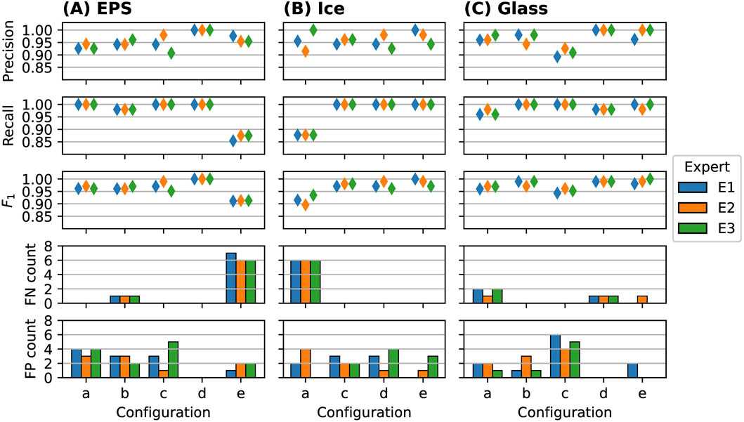
Figure 4. Scores to assess the model performance in terms of detection (1st row: precision, 2nd row: recall, 3rd row: $F_1$) and number of FN detections (4th row) and FP detections (5th row) of EPS (A), ice (B) and glass (C) hail objects in configurations a, b, c, d and e (surface of the test set, Figure 2), annotated by 3 different experts E1-E3 (colors). Note that the axis is cropped to only show the range [0.8, 1], while 1 corresponds to a perfect score. Over all experiments, a total of 250 EPS objects, 200 Ice objects and 251 glass objects have been placed. Note that for the glass objects, in one experiment 26 instead of the planned 25 objects were placed. Across all different types of objects, 7 objects (1.00%) were not visible (i.e., could not be annotated by the experts) in the orthophoto.

Figure 5

Figure 5. Sizes of FN (top row) and FP (bottom row) detections for hail object types EPS (A), ice (B) and glass (C) hail objects in all experiment configurations, annotated by 3 different experts E1-E3 (colors). The results are binned with a bin size of 10 mm. In the upper row (FN) the sizes are estimated based on the corresponding annotation, because the object was missed and the size of the object can only be inferred from the corresponding annotated object. Vice versa, the FP detections in the lower row are estimated based on the detection and do not have a corresponding annotation, and thus the size estimated based on the detections is shown. The binning is done because both, the detections and the annotations, are expected to not exactly correspond to the real size of the objects used in the experiments (with diameters 10, 15, 27, 32, 40, 60, 78 as shown in Table 2).

In the following, we present results for EPS hail objects, which allow us to assess detection performance across different size classes. Then, we report results for ice and glass hail objects, which are of uniform size.

4.1.1 EPS hail objects

In Figure 4A the model performance in terms of detection scores are shown for the EPS hail objects. The precision is in a range of 0.907-1.000, recall is in a range of 0.854–1.000 and the $F_1$ score is in a range of 0.911–1.000 across all experiment configurations.

The $F_1$ scores for all experts are above 0.95 for the configurations a–d, and above 0.85 for configuration e. Configuration e exhibits 6–7 FN, indicating missed hail objects by the model. This is also reflected in lower recall scores compared to the other experiment configurations. 1 to 5 FP detections were observed, indicating detections of objects without an annotated ground truth, in all experiment configurations except configuration d.

In Figure 5A the FN and FP detections depending on the size class are shown. All EPS hail objects above the 10–20 mm bin are correctly detected in all experiments (i.e., no FN), while most FP detections occur below 20 mm. The FP in the size bin of (50–60 mm) can be assign to a highly reflective leaf with a size of 57 mm in configuration a, which was falsely detected by the models of all experts. Overall, both FP and FN detections tend to occur for small size classes below 20 mm and fewer FN than FP detections can be observed, with rare FP detections of large objects as hail (e.g., leaves or flowers).

The results indicate that independent of the background, the ML-based model can detect EPS hail objects correctly with only few FP detections (below 5%) and even less FN detections (below 3%) across all surfaces. However for the surfaces with higher and more dense grass (experiment e) slightly enhanced FN detections thus lower the scores.

4.1.2 Ice and glass hail objects

In Figure 4B, the model performance in terms of detection scores for ice hail objects are shown. Similar to the EPS objects, the precision is above 0.9, recall is above 0.85 and the $F_1$ scores above 0.89 for all model configurations. For the experiment configuration a, the $F_1$ scores are dominated by 6 FN detections, indicating missed ice objects for the models for all experts. Note that for the ice objects, the experiment configuration b is not available due to a different setup during the data collection (see 2.2.3). In configurations c-e, all ice hail objects were correctly detected.

In Figure 4C, the model performance in terms of detection scores for glass hail objects are shown. As for EPS and ice objects, the precision is above 0.9, recall is above 0.95 and the $F_1$ scores above 0.94 for all model configurations. In general, the $F_1$ scores of the glass experiments are more consistent than the $F_1$ scores of the ice and EPS experiments, for which one experiment configuration exhibits lower $F_1$ scores (configuration e for EPS and configuration a for ice). Only a slight degradation of scores in configuration c can be observed for the glass objects.

4.2 Assessing model performance in terms of size estimation

To assess the model performance in terms of size estimation, the major axis determined from the detections of the hail objects is compared with two ground truths, the major axis estimation of the annotations and the real size of the objects. This allows estimate the uncertainty of the size estimation based on the visually determined annotation by including the real size of the objects which in real hail case are not available.

Similarly to Section 4.1, we first present results for EPS hail objects, followed by those for ice and glass hail objects.

4.2.1 EPS hail objects

Figure 6 shows the biases $\mathrm{\Delta }d$ grouped by experiment configurations in (A) and total in (B). The bias is computed with the annotations as a reference (light shade) and the real size as a reference (dark shade) for each expert. The magnitude of the biases in configuration a and b are below 1 mm with a spread of the IQR of 1–2 mm (black lines) for all experts, while the major axis tends to be overestimated compared to the real size but underestimated compared to the annotations. The bias in configurations c-e are slightly higher within the range −0.5 to −1.0 with a spread of about 2 mm and thus the detections tend to underestimate the major axis compared to both, the annotation and the actual real size of the objects. The biases are computed across all configurations and all sizes for the experts E1-E3 as bias $\pm$ standard-deviation (E1: (−0.41 $\pm$ 1.41) mm, E2: (0.03 $\pm$ 1.78) mm and E3: (−0.30 $\pm$ 1.48) mm). The relative biases do not show a different pattern but lie in a range of −10%–5%, with a mean bias around −5% (not shown).

Figure 6

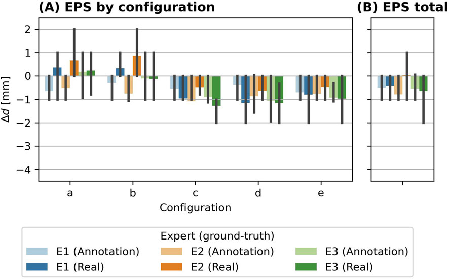
Figure 6. Bias $(\mathrm{\Delta }d)$ of detected major hail object axes compared to annotated major axes (light shade) and real major axes (dark shade) for each expert E1-E3 (colors) of TP detections. The black lines show the inter-quartile range (IQR). (A) The biases are grouped by configuration over all sizes. In each configuration (surface of the test set, Figure 2), there are a similar amount of annotations and detections. (B) Bias across all configurations and sizes.

Figure 7 presents the biases (top) and relative biases (bottom) of the EPS objects, grouped by shape (spherical and oval spheroid). In (A), the biases $\mathrm{\Delta }d$ are grouped by their real size classes over all experiment configurations with spherical EPS hail objects are shown. Similarly, the biases over all experiment configurations with oval spheroid EPS hail objects are shown in (B). The bias is computed with the annotations as reference (light shade) and the real size as reference (dark shade) for each expert. The horizontal grey bars represent the objects’ measured ranges as shown in Table 2. The bias for spherical objects with a size of $\le$40 mm is in the range of $\pm$1 mm) with a IQR spread of up to 2 mm), while the oval objects with larger sizes (60 mm and 78 mm exhibit a larger bias from −2.7  to 1.2 mm and the IQR spread is also increased, reaching values of up to 6 mm. The relative biases are shown for spherical EPS hail objects in (C) and for oval spheroid hail objects in (D). The largest relative biases are observed for the smallest size class (10 mm) with values reaching −8%. The relative bias is smallest in magnitude for the 40 mm size class, with values near 0%, but increases again for size classes $>$40 mm. Oval spheroid objects exhibit a substantially higher relative bias, approaching that of the 10 mm spherical EPS hail objects.

Figure 7

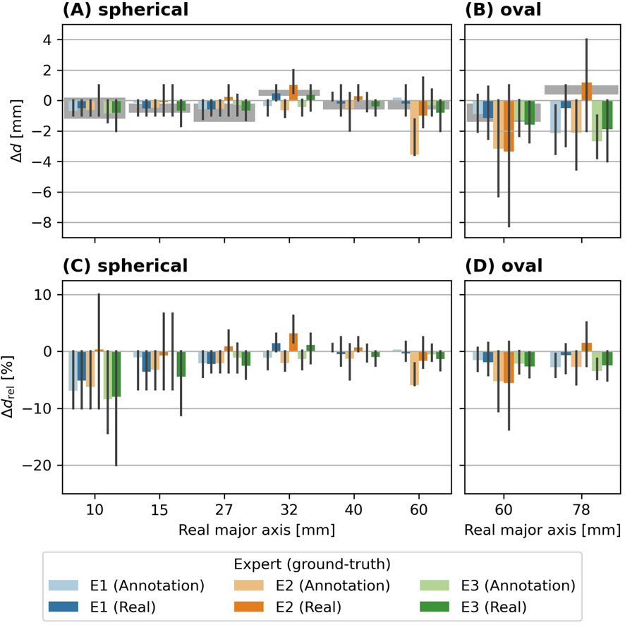
Figure 7. Bias $(\mathrm{\Delta }d)$ of detected major hail object axes compared to annotated major axes (light shade) and real major axes (dark shade) for each expert E1-E3 (colors) of TP detections. The black lines show the inter-quartile range (IQR). Top: absolute bias $\mathrm{\Delta }d$, the horizontal grey bars show the measured size as mean $\pm$ standard deviation (Table 2). Bottom: relative bias $\mathrm{\Delta }{d}_{\text{rel}}$. (A) biases of all EPS spheres ranging from 10 mm to 60 mm, grouped by size class. (B) biases of all EPS oval spheroid objects 60 mm and 78 mm, grouped by size class. (C) relative biases of all EPS spheres ranging from 10 mm to 60 mm, grouped by size class. (D) relative biases of all EPS oval spheroid objects 60 mm and 78 mm, grouped by size class.

4.2.2 Ice and glass hail objects

In Figure 8A, the bias $\mathrm{\Delta }d$ for ice and glass hail objects is shown. In contrast to the EPS objects, only one size was used and thus the bias can only be assessed as a function of the different experiment configurations. For the ice objects, largest biases are observed for experiment configuration a with biases between −3 mm and −2 mm against the real size as reference. The biases tend to be smaller in magnitude for experiment configuration a if the annotations are used as reference. In the other experiment configurations (c-e), the biases are in the order of −0.5 mm to −1 mm, and a tendency for larger biases in magnitude is prevalent if the real sizes are used as reference. The biases for the glass objects, shown in panel (C), are similar for all experiment configurations between −1 mm and −2 mm. Only in the experiment configuration c larger biases are observed, when the real sizes are used as a reference, whereas for the other experiments, the biases tend to be higher if the annotation size is used as a reference.

Figure 8

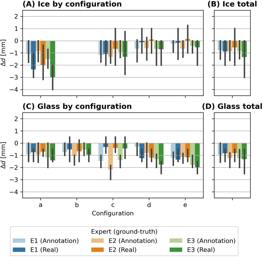
Figure 8. Bias of detected major hail object axes $(\mathrm{\Delta }d)$ compared to annotated major axes (light shade) and real major axes (dark shade) for each expert E1-E3 (colors). The black lines show the inter-quartile range (IQR). (A) Ice hail objects grouped by configuration, (B) ice hail objects cross all configurations (surface of the test set, Figure 2), (C) glass hail objects grouped by configuration, (D) glass hail objects across all configurations.

Regarding the difference between using the annotation or the real size as reference, the results indicate a complex behavior. In some experiments, the biases between the detected size and the real size are smaller than the biases between the detected size and the annotated size. This is the case for configurations a and b with EPS hail objects, for annotations from experts E1 and E2 (Figure 6), ice experiment d with annotations from expert E1 and E2, configurations c with glass hail objects for annotations of all experts. The occurrence of these larger biases in the annotations is not consistent for different types of hail objects, e.g., they appear in configuration a and b for EPS hail objects, but in configuration d for ice hail objects.

4.3 Direct comparison between annotated and real sizes

The major limitation of the ML-based approach to automatically retrieve the HSD from photogrammetric data is related to the absence of real ground truth data. The only ground truth that can be used is the manually annotated test dataset. The visual annotation is partially subjective to the expert and highly depends on the quality of the orthophoto. In the experiment setup for this study, the real ground truth is known, which allows to estimate an uncertainty of the annotations itself.

In Figure 9, the bias between the annotated major axes and the real major axes of EPS hail objects are shown. This bias corresponds to the difference between the dark and light bars from Figure 6. Across all EPS experiment configurations and sizes (panel (C)), the mean bias and the spread differ between the experts, but the biases between them is even smaller compared to the ML-based retrievals. E1 and E3 are very close to the real sizes with slight over- and underestimations, while E2 exhibits a more pronounced overestimation compared to the real size (E1: (0.09 $\pm$ 1.35) mm, E2: (0.82 $\pm$ 1.53) mm, E3: (−0.10 $\pm$ 1.43) mm). This highlights the subjectivity of annotations, as each expert has a different bias when annotating the same images. The subjective over- and underestimation also depends on the surface type, as shown in panel (A). Experts E1 and E2 tend to underestimate the real size for experiments a and b, whereas E1 and E3 tend to underestimate the size in configuration c-e. Similarly, for the real size classes, E2 tends to overestimate all sizes with the largest positive bias for large sizes, whereas E1 and E3 tend to underestimate the sizes for most size classes, shown in panel (B). Generally, the biases between the annotations and real sizes are smaller in magnitude than the biases of detected sizes compared to the references. E2 is an exception, where large annotations lead to a counteraction of the underestimation (compare Figure 6). A similar pattern was observed for ice (E1: (−0.11 $\pm$ 2.12) mm, E2: (0.31 $\pm$ 2.21) mm, E3: (−0.48 $\pm$ 1.98) mm) and glass (E1: (0.09 $\pm$ 1.34), E2: (0.41 $\pm$ 1.40), E3: (−0.08 $\pm$ 1.28)) (not shown). Across all types of hail objects, the biases between the references (annotated and real sizes) tend to be smaller in magnitude than the biases between both the detected and the real size as well as between the detected and annotated size.

Figure 9

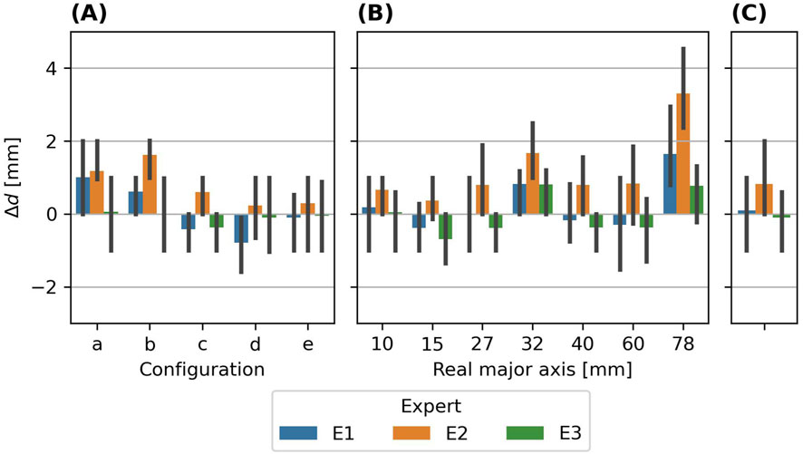
Figure 9. Biases $(\mathrm{\Delta }d)$ between annotated major axes and real major axes of EPS hail objects. The black bars show the IQR. (A) Biases grouped by configurations (surface of the test set, Figure 2), (B) Biases grouped by real size classes, (C) Biases across all experiments and size classes.

4.4 Real hail event

In addition to the experiments, data from a real hail event is used to assess the performance of the ML-based HSD retrieval in a real-world case. Figure 10 shows the processed orthophoto of the event described in Section 2.3, with masked areas as described in Section 3.1. The meadow on which the orthophoto was taken can be described as having irregular density, with medium to long grass and many clover flowers (most similar to experiment background e).

Figure 10

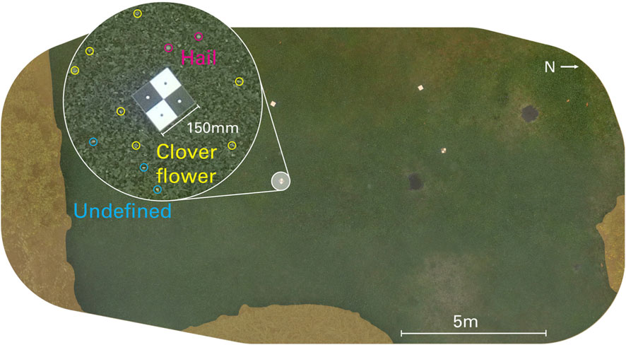
Figure 10. Orthophoto of the hail event surveyed on 28 June 2022 in Locarno-Monti (Switzerland) covering 220.2 m² and generated based on 44 individual drone images. The excerpt on the left shows the challenging conditions for annotation and detection due to low contrast and similar appearance of hail (magenta), flowers of clover (yellow) and other unknown objects (cyan). The excerpt also shows the ground control point (GCP) with a side-length of 150 mm. The orange areas indicate the masked areas such as tall grass, bushes and the GCPs, which do not show any hailstones. This area is filled with solid black color for detection, leaving 194.6 m².

In Figure 11, the scores to assess the model performance for the real hail event verified against the annotations in the test dataset of each of the experts are shown. In general, slightly lower scores compared to the experiments are achieved. Precision is in range of 0.69–0.81) (panel (A)), recall is in range of 0.77–0.83) (panel (B)) and the $F_1$ score is in the range between 0.75 and 0.82 (panel (C)). Regarding FP and FN detection depending on the size, the peak of FP detections is found between 6 mm and 8 mm, while there are no FP detections larger than 14 mm. There are fewer FN detections than FP detections (E1: 23, E2: 19 and E3: 31). The FP detections range from 4 mm to 14 mm for all models. Most FN detections are also between 6 mm and 8 mm, with only few FN detections $>$10 mm.

Figure 11

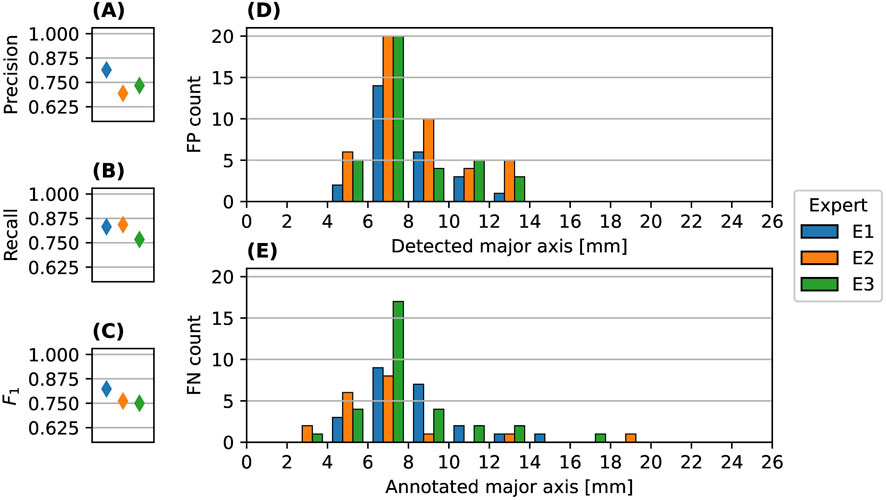
Figure 11. Scores to assess the model performance in terms of detection: precision (A), recall (B), $F_1$ (C) and number of FP detections (D) and FN detections (E) of the real hail event annotated by 3 different experts E1-E3 (colors). Note that the axis is cropped to only show the range [0.55, 1] (different from Figure 4), while 1 corresponds to a perfect score.

In Figure 12, the retrieved HSD are shown for the annotations in the test dataset in panel (A), for the detections in the test dataset in panel (B), and for the detections in the full dataset including train, validation and test in panel (C). The total number of detections in the full set are for the experts E1: 4087, E2: 4420, E3: 4180. The annotations in the test dataset range from 3 mm to 18 mm, while the detections in the test dataset range from 4.5 mm to 15 mm. The peak of the HSD of the annotations in the test dataset are for all models between 10 mm and 12 mm, while the peak of the detections in the test dataset is shifted to slightly smaller major axes between 8 mm and 10 mm, which is similar to the peak of the detections of the full dataset. The HSD of annotations (A) is wider than the HSD of the detections (B), partially due to the FN detections $>$14 mm by the models of all experts (Figure 11E). The model of expert E1 performs better than the models of E2 and E3, as indicated by the higher $F_1$ score, as well as lower FP and FN counts and no larger ($>$16 mm) hailstones missed. The KDEs of the full dataset (panel (C)) show good agreement between the models from different experts in the range of 6 mm–14 mm, while there is more agreement between E2 and E3 below that range and more agreement between E1 and E3 above it. All models agree on the largest size of around 24 mm.

Figure 12

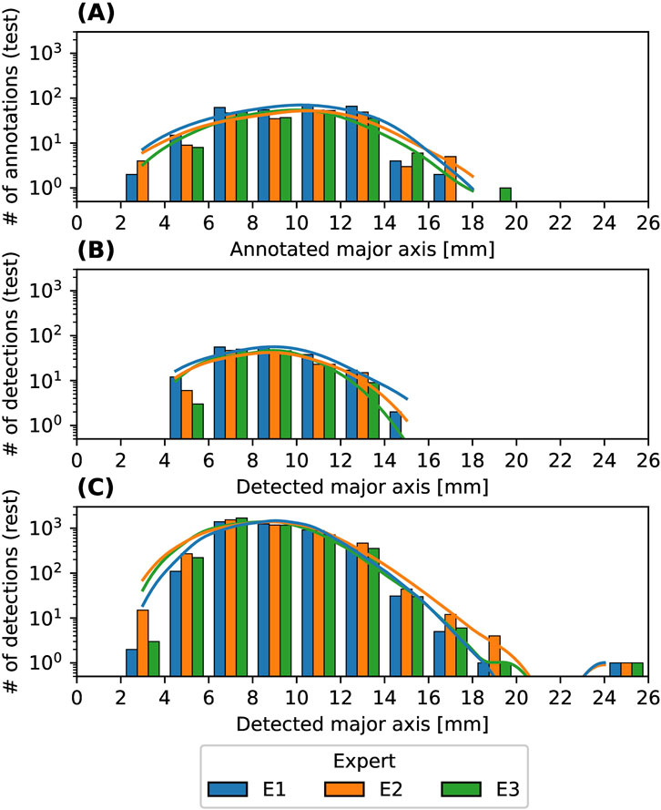
Figure 12. HSD of the hail event on a logarithmic scale in bins of 2 mm. The lines show the kernel density estimation (KDE). (A): HSD of the annotations in the test dataset, (B): HSD of detections in the test dataset, (C): Detections in the full dataset, including training, validation and test.

Figure 13, shows the biases between the experts annotations and the model detections of the hail event in the test dataset, grouped by their annotated major axes in 2 mm bins from 2 mm to 18 mm in panel (A), and across all sizes in panel (B). Only TP detections can be analyzed, since FN are not detected and FP do not have an annotation to compare against. There is a single detection in the bin 16 mm–18 mm, which is estimated with a bias of nearly 3 mm, thus, it shows up in the 12–14 mm bin in Figure 12. For the number of detections in each bin of the test dataset, refer to Figure 12A. Over all sizes, the biases for the models of the experts are E1: (−0.84 $\pm$ 1.36) mm, E2: (−0.16 $\pm$ 1.50) mm, E3: (−1.22 $\pm$ 1.47) mm, which are comparable to the biases found in the experiments, but the difference between the experts is more pronounced. Compared to the 10 mm and 15 mm EPS hail objects from the experiments, the biases of the hail event do not follow the same characteristics. The biases for small EPS hail objects are smaller than for large EPS hail objects, but there is only a small difference between 10 mm and 15 mm hail objects. Since the experiments lack hail objects below 10 mm, there is no comparison available for these small sizes from the experiments.

Figure 13

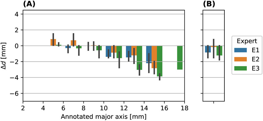
Figure 13. Bias of detected major hail object axes $(\mathrm{\Delta }d)$ compared to annotated major axes for each expert E1-E3 (colors). The black lines show the IQR, if at least two values are present in the bin. (A) biases grouped into 2 mm bins, (B) biases across all sizes.

5 Discussion

The results show that small hail objects were more frequently missed on taller grass. Similar results were obtained for different types of hail objects, with some differences in individual experiments. The sizes of the hail objects were estimated with only a small underestimation and slight variations depending on the experts annotations for the model training. Previous research (Soderholm et al., 2020; Lainer et al., 2024) showed promising results from drone-based hail photogrammetry, but could not accurately quantify the errors of the method, due to a lack of a known ground truth. We also compared the results from the synthetic hail experiments to a real hail event, where we found slightly larger biases and reduced detection performance for real hailstones due to challenging light conditions.

The experiments conducted in this study allowed us to quantify the performance of drone-based hail photogrammetry coupled with ML, in detecting synthetic hail objects of various types and retrieve their size classes on different grass surfaces. In this section, we first highlight the key factors influencing the model’s performance (Section 5.1) based on the findings from the experiments. Then these findings and their implications for real hail events are discussed in (Section 5.2). Finally, we address the limitations of our experimental setup and suggest areas for improvement (Section 5.3).

5.1 Factors influencing the model performance

In terms of detecting synthetic hail objects, the models perform well, independent of the type of synthetic hail object used (EPS, glass, ice) with a $F_1$ score $>$0.95 for most configurations. This indicates that drone based HSD retrievals are overall highly accurate and able to correctly detect individual synthetic hail objects. However, with backgrounds exhibiting long grass (experiment e) slightly lower scores in terms of detection are reached for EPS hail objects, but not for ice and glass objects. This is likely related to EPS hail objects partially or fully hidden by the grass. This can be related to the positioning of the EPS hail objects, which were fixed to the ground using wooden toothpicks. Therefore some small size EPS objects ($\le$15 mm) were placed lower in the grass to imitate the position in real hail events. In contrast, ice and glass objects were of uniform size and mostly stayed on top of the grass and were thus less prone to be covered by longer grass.

The translucent characteristics of real hail can pose significant challenges for the identification of hailstones in the orthophoto for both human experts and ML models by lowering the lightness as reported by Lainer et al. (2024). To imitate the translucency of real hail, ice and glass objects were used. In particular for configuration a with the ice hail objects, a higher number of missed objects is observed, which can be attributed to more translucent ice. This particular setup of configuration a (Section 2.2.2) lead to longer melting times compared to the other configurations of the experiments with ice objects. Therefore, the lowered performance is likely explained by more translucent ice objects.

Similarly, in experiments with glass, configuration c exhibits a higher number of FP detections. This can be attributed to an interplay between lower light availability due to a cumulus clouds passing above the survey area and the translucent characteristic of glass hail objects. The reduction in sunlight lowered the image quality and therefore the contrast of the glass hail objects in the orthophoto. Under these environmental conditions, the (translucent) glass hail objects exhibit similar characteristics as non-hail objects (i.e., clover flowers and bright stones). Therefore, more FP detections can occur. This effect was not observed for experiments with EPS and ice hail objects, where no clouds were present.

Based on the experiments with the EPS hail objects, the performance of detection was further assessed according to the size of the objects. Generally, missed hail objects (i.e., FN counts) tend to be of smaller size ($\le$15 mm), while misclassified non-hail objects (i.e., FP counts) can also be large objects, such as a highly reflective leaf with an axis of around 57 mm, which was identified as hail by the models of all experts one configuration a with EPS hail objects. Therefore, it is important to manually check the largest detections for FP detections manually and remove non-hail objects from the final HSD, such that the largest size reported is actually hail. Furthermore, on site observations during the data collection procedure should be carefully documented to be aware of objects that might be misclassified (e.g., leaves or flowers). In some configurations, perfect $F_1$ scores of 1.00 were achieved, indicating perfect model performance. This is likely attributed to the nature of the experiments representing best-case scenarios and limited number of hail objects and thus can likely not directly be transferred to real hail events.

Beside the detection itself, a correct estimation of the retrieved size of the detections is crucial for further use of such data. The performance of the size estimation in EPS experiments overall yields a small underestimation of less than 1 mm when compared to both, the real and the annotated sizes, with only small variations between the experts. This indicates that the retrieved HSD overall closely follows the real HSD. But the bias depends on the actual size and shape of the EPS hail objects, where larger absolute biases are found for large oval spheroid hail objects. In relative terms, the largest biases are observed for small EPS hail objects ($\le$15 mm). To further translate those error estimates from EPS hail objects to real hail events, the biases found for ice and glass hail objects are taken into account. For those transparent objects, the biases are generally higher compared to the same size of EPS objects. Thus the translucent characteristics of hail—which is imitated by the ice and glass objects—tends to increase the errors. For the ice objects with a size of around 25 mm, the errors are up to 3 mm, whereas the EPS objects of 27 mm indicate errors below 1 mm. Similarly, glass objects with a size of 19.5 mm exhibit errors up to 2 mm, whereas the errors for EPS objects of similar size are smaller than 1 mm. Thus the uncertainty in the retrieved HSD estimation for a real event will likely be increased compared to the findings based on the experiments with EPS objects. Another aspect, in particular for ice objects, is related to the melting. As discussed above for the performance regarding the detections, ice hail objects show a more pronounced underestimation for configuration a, which can be attributed to the different setup and longer flight time, what leads to longer melting an therefore to smaller ice hail objects during the data collection. If configuration a is excluded from the analysis, the biases still tend to be larger compared to EPS hail objects, but similar to the glass hail objects. In comparison to existing methods for hail size estimations on the ground, automatic hail sensors use size classes of 5 mm due to uncertainties related to the estimation of the kinetic energy of up to 20%, which are reported by the manufacturer (Kopp et al., 2023a). Thus, the biases found for EPS hail objects in the experiments, as well as the increased errors found based on ice and glass objects are comparable to the uncertainties of automatic hail sensors and can therefore be a valuable complementary data source.

The third aspect is related to the annotation process of the hail objects in the orthophoto. The annotations among the three experts indicate differences of up to 2 mm for the largest EPS size class, but depending on the background (i.e., experiment configuration) the biases show only small variations between the experts. These biases are in a similar range as the biases between the size of the detection (model retrievals) and the size of the annotations and the real sizes respectively.

Subjectivity of annotations also has an influence on the final model predictions. For example, annotations from expert E2 were larger than the real object’s sizes and annotations from other experts. The ML model trained with annotations from E2 showed less underestimation of object sizes compared to models trained with annotations from other experts, with some instances even showing overestimation. Thus, this resulted in a smaller bias compared to the real sizes, showing that under these circumstances, a higher performance can be achieved on inaccurate annotations.

Thus the differences between the experts are small, but they still highlight the subjectivity of the annotations and the importance of quantifying the accuracy of the annotations that are used to train the ML models. We suggest to place some hail-like reference objects (such as the synthetic hail objects used in this study) in the survey area during the data collection, which allows to quantify the uncertainty associated to the annotation process from different experts.

5.2 Implications of synthetic hail experiments for application to real hail events

In the real event, slightly reduced $F_1$ scores for detection and slightly increased biases in size estimation were observed compared to the experiments with synthetic hail objects. Both recall and precision are lower compared to the experiments, as a result of more FP and FN detections. Overall the biases between the detected size and the annotations in the real event are larger (up to 4 mm) compared to the biases estimated based on the EPS experiments, but is in good agreement when the biases of the ice and glass experiments are taken into account. In the real event, biases in size estimation show a tendency to increase towards larger hailstones (10–20 mm) (note that the largest annotation is 20 mm). Likewise for the EPS experiments, increased biases are found mainly for large hail objects. The larger biases are only apparent at sizes of $\ge$60 mm for the EPS experiments, while the 10–27 mm EPS objects tended to be underestimated. This increase of the bias towards larger objects in the HSD can be related to two factors. Firstly, in the real event the number of large hailstones is much lower than the number of small hailstones, which leads to higher uncertainties for large hailstones. This distribution is also present by design for the synthetic hail objects. Secondly, this observation could partially be explained with an inherent bias of the ML models towards a center size (mean around 9–10 mm in the real event, depending on the expert) for all hailstones or hail objects in the training set, meaning that small hailstones were overestimated and large hailstones were underestimated. This could partially be observed for EPS hail objects in the experiments as well. However, this effect was already apparent at 14–16 mm with hailstones, while the experiments with EPS exhibited it only for oval spheroid objects with sizes $\ge$60 mm, while the smallest size classes still tended to be underestimated. Further examination of this effect is necessary and other models could be examined to better understand and quantify this effect. The biases of the experts’ annotations should also be taken into account to separate their effects from the model biases.

The real hail event discussed here is a representative case that highlights the challenges of hail photogrammetry. The low light conditions during the thunderstorm leading to reduced contrast of hail in the photogrammetric data and clover flowers make detection more challenging compared to the experimental setup. The detection performance score in the test dataset $F_1$ = 0.75, is of the same order of the score reported in Lainer et al. (2024) ($F_1$ = 0.80) for a different event. The exact number of hailstones and the minimum survey area required for a representative HSD depend on the specific conditions of the event. Soderholm et al. (2020) estimated that a survey area of 40.1 m², containing 2,088 hailstones, is sufficient based on their observed distribution. In our case, approximately 4,000 hailstones were detected in the orthophoto, suggesting that a representative estimation of the HSD is achievable. In comparison, Lainer et al. (2024) detected around 18,000 hailstones, which reflects the significantly larger survey area of 750.4 m², as opposed to our 194.6 m². In Lainer et al. (2024) only the test dataset was annotated by 3 experts, here we annotated all datasets (training, validation and test) by 3 experts. This allows to assess differences in the final HSD distribution, retrieved by the models trained with the dataset from the different experts. In the test dataset, similar variations between the models of the experts are observed, as for the event analyzed by Lainer et al. (2024). Additionally the variations in the final HSD for all experts are similar, which indicates that the retrieved HSD are robust despite the subjective annotation process. Overall, these biases with respect to the annotations in the real event are larger in magnitude (up to 4 mm) compared to the biases with respect to the annotations in the EPS experiments ($>$1 mm) and as well compared to biases for the ice and glass experiments ($>$2 mm). Thus we conclude that in case of real events, the uncertainty of the size estimation increases, but are similar to the uncertainties obtained with other ground observation systems (e.g., automatic hail senors).

Based on the results with synthetic hail objects, we recommend to perform surveys on surfaces with short and uniform grass cover, with a minimum amount of flowers or other objects that could be mistaken for hail. Additionally, a minimum delay between the last falling of hail and the start of the survey is crucial for high quality data. These strategies were already mentioned in Soderholm et al. (2020) and supported by our experiments. Surveys on different surfaces such as asphalt could also be considered, but exhibit other problems, including the washing away of hailstones by liquid precipitation, increased melting rates due to the likely warmer ground, as well as shattering of hailstones on impact. These are however only hypotheses and would need to be evaluated further.

In the real event presented in this study, hail was followed by strong winds and intense rain. Therefore, the data collection using the drone started roughly 20 min after the hail strike ceded, time during which the hailstones continued to melt. Research on the melting behavior of hailstones focuses on the atmosphere (e.g., Fraile et al., 2003). Investigation of hailstones melting on the ground was first performed in Lainer et al. (2024) using drone-based photogrammetry. Assuming the same hypothetical melting rate of 0.5 mm/min during the delay between the end of the hail strike and start of the survey (18.65 min in Lainer et al. (2024)), we estimate the largest size of about 35 mm for the largest hailstones at the time of the photogrammetry flight. This estimation is within the order of the reports from the crowd-sourced data of 20–30 mm in a radius of 2 km, even though the same melting rate is not directly applicable to the event in Locarno due to different environmental conditions (such as temperature, humidity, wind, grass, hailstone size). The melting of the event in Lainer et al. (2024) was observed at ambient temperatures of around 20 °C with relative humidity around 85%, while the melting of the event in Locarno was observed around 17 °C at a relative humidity between 90 % and 100%. Further experiments to assess melting behavior of hailstones on the ground, such as presented in Lainer et al. (2024), under different ambient conditions would be of high value.

The objects in the experiments are more distinct compared to the hailstones in the real event, but even under ideal conditions, there was some disagreement in the annotations between experts. The uncertainty of the annotations in the real event is considerably higher, as it is impossible to know if the annotations are correct. This means that, by accident, a model could be trained that detects both clover leaves and hail, because the annotations include annotations of clover flowers as hail, leading to high $F_1$ scores, while detecting a large proportion of clover leaves as hail. Therefore it is helpful for the experts to know the conditions during the event at the survey site to increase the confidence when annotating. However, even with this uncertainty, the models of all experts agree on the largest hailstone (with a size of 25 mm) and the resulting HSDs have similar shapes. The lower tail of the HSD is most prone to false detections, since small objects are harder to identify for both human experts and the ML models, as shown in the experimental setup. Since hailstones $>$5 mm are not considered as hail (American Meteorological Society, 2025), this could serve as threshold for inclusion, which is also used for data from the automatic hail sensors (Ferrone et al., 2024).

5.3 Limitations and uncertainties in the experimental setup

For the size comparison of EPS objects, we used the reference size reported by the manufacturer. To confirm the reported sizes, the objects were measured in the lab and revealed slightly deviating axes than reported. We found that the deviation from the reported manufacturer’s sizes (Table 2) correlates with the biases found in EPS experiments (Figure 6). For example, 32 mm EPS hail objects were overestimated by the models, while also being larger than the manufacturer’s size. However, the used objects vary by up to 0.7 mm in size within a size class. To eliminate the influence of the varying object’s axes, the experiments should be repeated with calibrated objects in future studies.

The larger biases observed for oval spheroid EPS objects (Figure 7) can be partly attributed to deviations from the manufacturer’s reported sizes. However, only the 60 mm objects are smaller than specified (grey cell in Table 2), while the 78 mm objects tend to be larger than the manufacturer’s specification. Another factor explaining the larger biases, is the fitted bounding box being slightly rotated to the major and minor axes of the object, since the algorithm tries to minimize the area of the bounding box. In case of low axis ratios, the major axis gets underestimated and the minor axis gets overestimated. Additionally, the subjectivity of the annotation process might again play a role here. It was observed that coarse annotations influenced the resulting bounding box more than for spherical objects. For events with hailstones with low axis ratios (i.e., non-spherical), the current approach might need to be improved to correctly estimate the axes.

Another limiting factor is that the optimal threshold for the ML detection (Section 3.4) was determined based on the test dataset, which could lead to overfitting, since we optimize the model to the conditions of the test set. Due to the design of the LOOCV, it is not suitable to set the thresholds based on the validation dataset, as the validation dataset is constructed based on the data from all surfaces except the surfaces used for the test dataset. Setting the threshold based on the test dataset means that the detection scores represent a best-case scenario and real-world applications are expected to perform slightly worse, which is confirmed by the observations from the real hail event.

We noticed that in certain experiment configurations, hail objects were hidden in the corresponding orthophoto. Overall, this corresponds to only 1% of placed hail objects, only affecting EPS hail objects $\le$15 mm. The amount of hidden objects mostly depends on the length of grass, with most hidden hailstones present in configuration e. Therefore, we highly recommend to avoid surfaces with long grass ($>$30 mm) and be aware that the lower tail of the HSD is affected by such invisible hailstones. Currently, we cannot accurately account for hidden hailstones in real hail events, since in this case the distribution of hidden hailstones is unknown. A suggested solution could be to count hailstones in a predefined area (i.e., 1 m²) in the filed prior to performing the survey. The ratio of hailstones counted in field to annotated hailstones in the orthophoto could be used to estimate the ratio of hidden hailstone over the entire survey area (Soderholm et al., 2020). This ratio could be used to estimate the amount of hidden hailstones more accurately.

The scores reported need to be interpreted using detailed expert knowledge about the event, the surface and the environmental conditions. In particular for photogrammetric data from real events, a high $F_1$ score alone does not automatically mean that a model is well trained to detect hail. The experts annotating the dataset may encounter uncertainty in classifying objects as hail, which is hard to quantify (e.g., clover, leaves, other objects), meaning that the annotated ground truth is not representative. In the experiments, the distribution and number of the hail objects are known and thus we have high confidence in the annotations and by extension in the reliability of the resulting $F_1$ scores to indicate model performance. However, for real hail events, where a ground truth is absent, faulty annotation of non-hail objects by experts cannot be excluded.

In the experiments, the aperture of the lens varies between $f/4$ and $f/8$, while for the real event it is fixed at $f/2.8$. An open aperture (low f-number) leads to decreased optical resolution, but allows for shorter exposure times, since more light reaches the sensor. This allows us to reduce the exposure time, limiting motion blur. A trade-off between optical resolution (aperture opening and lens characteristics), motion blur (exposure time) and noise (ISO value) is always present for photogrammetric data capture. More events and experiments with systematic variation of these parameters under different conditions need to be analyzed to accurately quantify these effects in practical terms. The theoretical uncertainties that arise from the GSD are 1 mm/px for the synthetic hail experiments and 1.5 mm/px for the real hail event, from motion blur are 1 mm for the synthetic experiments and 2.67 mm for the real hail event. Additionally, the uncertainty in scaling the orthophoto is around 5% (measurements accurate only to 2–3 px). These uncertainties are similar or larger than the magnitude of the bias ($\le$2 mm for ice and glass hail objects, $\le$1 mm for EPS hail objects) in the estimated major axes for the synthetic hail experiments under ideal conditions—compared to the measured real major axes of the synthetic hail objects. The uncertainties found from this study are generally small in regard to the application of verifying radar estimates, where POH and MESHS are measured in cm.

6 Conclusion and outlook

Drone-based hail photogrammetry shows promising potential to retrieve accurate HSDs of hail on the ground, which provide valuable data that can complement existing ground observation systems. While previous studies applied this approach, a systematic comparison against a known ground-truth HSD was lacking. Our experiments with synthetic hail objects of known sizes addressed this gap by assessing the performance of drone-based photogrammetry coupled with ML, in detecting and estimating the size of individual hail objects on different types of grass.

Overall, the type of grass cover only had a small impact on the performance, but the length of the grass affected the detection of small hail objects. A comparison to the performance of this approach applied to a real event revealed that the real-world conditions pose greater challenges for hail detection and size estimation. Despite these challenges, our results indicate that drone-based retrievals of real hail provide reliable HSD retrievals. Further, we improved several aspects of the hail photogrammetry process by combining the advantages of Soderholm et al. (2020), such as using a overlapping area to prevent cutting off hail, and the advantages of Lainer et al. (2024), such as using the R-CNN model for direct size estimation.

The key results from our experiments with artificial hail objects and the real hail event are the following:

$•$ There are only small differences between the types of artificial hail in terms of detection and size estimation

$•$ Large hail objects were detected correctly, but smaller hail objects are harder to detect

$•$ The estimated sizes of the hail objects in the experiments agree well with the ground truth (with $\mathrm{\Delta }d$ in the order of −0.75 mm)

$•$ Experiments on different grass types lead to similar results, but long grass leads to more hidden hail objects in the orthophoto and thus missing in the HSD

$•$ Detection of hailstones in the orthophoto of the real event is more challenging due to lower contrast as a result of low light conditions and melting

$•$ The bias between annotated sizes of the real hailstones are slightly larger in magnitude compared to the experiments but overall remain small

$•$ Annotation styles vary among experts, leading to small but systematic differences in the trained models

These results demonstrate the reliability of drone-based HSD retrievals and serve as a evaluation framework for further improvement.

However, there are limitations that were not assessed in this study, such as the melting of hail on the ground and the model performance on surfaces other than grass. A key limitation remains the dependence on natural light. The experiments were conducted during bright sunlight conditions, which is usually not the case during hail producing thunderstorms. An artificial light source on the drone or at the survey site would thus be highly valuable to extend the applications of drone-based hail photogrammetry. During the design of the experiments, we considered using the DJI Zenmuse H20T (DJI, 2020b) infrared (IR) camera. However, the limited resolution of 640 px$\times$521 px, it is unsuitable for hail photogrammetry. Since then, DJI released the Zenmuse H30T (DJI, 2024), quadrupling the resolution to 1280 px$\times$1024 px, resulting in a GSD of around 4 mm/px. Further advances in IR hardware could enable photogrammetry in the infrared spectrum, reducing the reliance on visible light. But currently, thermal cameras have greatly reduced image resolutions and are very costly.

To better understand the performance under real conditions, more surveys of real hail events would be highly valuable. In addition to the recommendations from Lainer et al. (2024), we suggest to add reference hail objects, such as used for the experiments, in the area of the orthophoto. These reference objects should be annotated the same way as hailstones, and the annotated sizes should be compared to the reference values. The LOOCV showed low dependency on the training data in terms of surface type, as long as the hail objects were visible. Experiments used the same objects and were conducted under similar conditions in terms of light (bright daylight). During real events, these parameters are likely to vary. Therefore, we recommend to train models using event-specific data. With more hail data becoming available from real events in the future, training a single, generalizable model for different events and surfaces may become feasible.

Although drone-based hail photogrammetry will likely not be useful in an operational manner, it could provide invaluable data when combined with other hail measurement devices, such as hailpads and automatic hail sensors. In particular, hailpads or compact radar systems for measuring fall speeds of hailstones (e.g., Gartner and Brimelow, 2024) could be deployed quickly in the field during a drone survey. A combination of these instruments could be highly beneficial for field campaigns, where different types of measurement devices are concentrated in a small area to observe hail at different stages from formation to the impacts on the ground and as a representative ground-truth for the validation of polarimetric weather radar products.

Data availability statement

Data of the event in Locarno-Monti can be found under lainer_hail_lom (Lainer, 2024) and and data of the experiments under portmann_experiments_2025 (Portmann and Lainer, 2025). Python codes used for analysis and generation of figures are available on (GitHub) portmann_ehw_code_2025 (Portmann and Lainer, 2025).

Author contributions

JP: Formal Analysis, Writing – original draft, Visualization, Project administration, Methodology, Software, Investigation, Validation, Conceptualization, Data curation, Writing – review and editing. ML: Conceptualization, Data curation, Formal Analysis, Investigation, Methodology, Software, Supervision, Validation, Writing – review and editing. KB: Conceptualization, Methodology, Supervision, Writing – review and editing. MJ: Data curation, Validation, Writing – review and editing. MG: Data curation, Validation, Writing – review and editing. SM: Conceptualization, Methodology, Project administration, Supervision, Validation, Writing – original draft, Writing – review and editing.

Funding

The author(s) declare that financial support was received for the research and/or publication of this article. The work of KB was funded by the Swiss National Science Foundation (SNSF) Sinergia grant CRSII5_201792.

Acknowledgments

The authors would like to thank Joshua Soderholm for the continued scientific exchange. We would also like to thank Alessandro Hering for input on the experimental design.

Conflict of interest

The authors declare that the research was conducted in the absence of any commercial or financial relationships that could be construed as a potential conflict of interest.

Generative AI statement

The author(s) declare that no Generative AI was used in the creation of this manuscript.

Any alternative text (alt text) provided alongside figures in this article has been generated by Frontiers with the support of artificial intelligence and reasonable efforts have been made to ensure accuracy, including review by the authors wherever possible. If you identify any issues, please contact us.

Publisher’s note

All claims expressed in this article are solely those of the authors and do not necessarily represent those of their affiliated organizations, or those of the publisher, the editors and the reviewers. Any product that may be evaluated in this article, or claim that may be made by its manufacturer, is not guaranteed or endorsed by the publisher.

Footnotes

¹Model weights from https://github.com/facebookresearch/detectron2/blob/main/configs/COCO-InstanceSegmentation/mask_rcnn_R_50_FPN_3x.yaml

References

Allen, J. T., and Tippett, M. K. (2021). The characteristics of United States hail reports: 1955-2014. E-J. Severe Storms Meteorol. 10, 1–31. doi:10.55599/ejssm.v10i3.60

CrossRef Full Text | Google Scholar

American Meteorological Society (2025). “Hail,” in Glossary of meteorology. Available online at: https://glossary.ametsoc.org/wiki/Hail.

Google Scholar

An, P., Yong, R., Du, S., Long, Y., Chen, J., Zhong, Z., et al. (2025). Potential of smartphone-based photogrammetry for measuring particle size and shape in field surveys. Bull. Eng. Geol. Environ. 84, 238. doi:10.1007/s10064-025-04246-7

CrossRef Full Text | Google Scholar

Barras, H., Hering, A., Martynov, A., Noti, P.-A., Germann, U., and Martius, O. (2019). Experiences with >50,000 crowdsourced hail reports in Switzerland. Bull. Am. Meteorological Soc. 100, 1429–1440. doi:10.1175/BAMS-D-18-0090.1

CrossRef Full Text | Google Scholar

Battaglioli, F., Groenemeijer, P., Púčik, T., Taszarek, M., Ulbrich, U., and Rust, H. (2023). Modeled multidecadal trends of lightning and (very) large hail in Europe and North America (1950–2021). J. Appl. Meteorol. Climatol. 62, 1627–1653. doi:10.1175/JAMC-D-22-0195.1

CrossRef Full Text | Google Scholar

Besic, N., Figueras I Ventura, J., Grazioli, J., Gabella, M., Germann, U., and Berne, A. (2016). Hydrometeor classification through statistical clustering of polarimetric radar measurements: a semi-supervised approach. Atmos. Meas. Tech. 9, 4425–4445. doi:10.5194/amt-9-4425-2016

CrossRef Full Text | Google Scholar

Bradski, G. (2000). The OpenCV library. Dr. Dobb’s J. Softw. Tools. 2236121.

Google Scholar

Brimelow, J. C., Kopp, G. A., and Sills, D. M. L. (2023). “The northern hail project: a renaissance in hail research in Canada,” in 11th European conference on severe storms, 41–50. doi:10.5194/ecss2023-170

CrossRef Full Text | Google Scholar

CVAT.ai Corporation (2023). Computer Vision Annotation Tool (CVAT). Available online at: https://github.com/cvat-ai/cvat.

Google Scholar

Dessens, J., Berthet, C., and Sanchez, J. (2007). A point hailfall classification based on hailpad measurements: the anelfa scale. Atmos. Res. 83, 132–139. doi:10.1016/j.atmosres.2006.02.029

CrossRef Full Text | Google Scholar

Ding, J., Wang, J., Yang, W., and Xia, G.-S. (2021). “Object detection in remote sensing,” in Deep learning for the Earth sciences (John Wiley and Sons, Ltd), 67–89. doi:10.1002/9781119646181.ch6

CrossRef Full Text | Google Scholar

DJI (2020a). Matrice 300 RTK.

Google Scholar

DJI (2020b). Zenmuse H20T.

Google Scholar

DJI (2021). Zenmuse P1

Google Scholar

DJI (2024). Zenmuse H30T.

Google Scholar

Federal Office of Topography swisstopo (2023). swissSURFACE3D raster.

Google Scholar

Federer, B., Waldvogel, A., Schmid, W., Schiesser, H. H., Hampel, F., Schweingruber, M., et al. (1986). Main results of grossversuch IV. J. Appl. Meteorology Climatol. 25, 917–957. doi:10.1175/1520-0450(1986)025<0917:mrogi>2.0.co;2

CrossRef Full Text | Google Scholar

Ferrone, A., Kopp, J., Lainer, M., Gabella, M., Germann, U., and Berne, A. (2024). Double-moment normalization of hail size number distributions over Switzerland. Atmos. Meas. Tech. 17, 7143–7168. doi:10.5194/amt-17-7143-2024

CrossRef Full Text | Google Scholar

Fraile, R., Castro, A., López, L., Sánchez, J. L., and Palencia, C. (2003). The influence of melting on hailstone size distribution 67-68, 203–213. doi:10.1016/S0169-8095(03)00052-8

CrossRef Full Text | Google Scholar

Gartner, M., and Brimelow, J. (2024). “The effectiveness of a continuous-wave radar to measure the fall speed of hailstones,” in 4th European hail workshop, 98.

Google Scholar

Gebäudeversicherung Luzern (GVL) (2022). Hagelereignis überschattet das Geschäftsjahr 2021.

Google Scholar

Germann, U., Boscacci, M., Clementi, L., Gabella, M., Hering, A., Sartori, M., et al. (2022). Weather radar in complex orography. Remote Sens. 14, 503. doi:10.3390/rs14030503

CrossRef Full Text | Google Scholar

Grazioli, J., Leuenberger, A., Peyraud, L., Figueras i Ventura, J., Gabella, M., Hering, A., et al. (2019). An adaptive thunderstorm measurement concept using C-Band and X-Band radar data. IEEE Geoscience Remote Sens. Lett. 16, 1673–1677. doi:10.1109/LGRS.2019.2909970

CrossRef Full Text | Google Scholar

Groos, A. R., Bertschinger, T. J., Kummer, C. M., Erlwein, S., Munz, L., and Philipp, A. (2019). The potential of low-cost UAVs and open-source photogrammetry software for high-resolution monitoring of alpine glaciers: a case study from the kanderfirn (Swiss alps). Geosciences 9, 356. doi:10.3390/geosciences9080356

CrossRef Full Text | Google Scholar

He, K., Zhang, X., Ren, S., and Sun, J. (2016). “Deep residual learning for image recognition,” in Proceedings of the IEEE conference on computer vision and pattern recognition (CVPR).

Google Scholar

He, K., Gkioxari, G., Dollár, P., and Girshick, R. (2018). Mask R-CNN. arXiv.org. doi:10.48550/arXiv.1703.06870

CrossRef Full Text | Google Scholar

Hering, A., and Betschart, M. (2012). Automatic hail detection at MeteoSwiss - Verification of the radar-based hail detection algorithms POH, MESHS and HAIL. Tech. Rep. 238.

Google Scholar

Hering, A. M., Morel, C., Galli, G., Sénési, S., Ambrosetti, P., and Boscacci, M. (2004). Nowcasting thunderstorms in the alpine region using a radar based adaptive thresholding scheme, 206–211.

Google Scholar

Hulton, F., and Schultz, D. M. (2024). Climatology of large hail in Europe: characteristics of the European severe weather database. Nat. Hazards Earth Syst. Sci. 24, 1079–1098. doi:10.5194/nhess-24-1079-2024

CrossRef Full Text | Google Scholar

Kopp, J., Manzato, A., Hering, A., Germann, U., and Martius, O. (2023a). How observations from automatic hail sensors in Switzerland shed light on local hailfall duration and compare with hailpad measurements. Atmos. Meas. Tech. 16, 3487–3503. doi:10.5194/amt-16-3487-2023

CrossRef Full Text | Google Scholar

Kopp, J., Schröer, K., Schwierz, C., Hering, A., Germann, U., and Martius, O. (2023b). The summer 2021 Switzerland hailstorms: weather situation, major impacts and unique observational data. Weather 78, 184–191. doi:10.1002/wea.4306

CrossRef Full Text | Google Scholar

Kopp, J., Hering, A., Germann, U., and Martius, O. (2024). Verification of weather-radar-based hail metrics with crowdsourced observations from Switzerland. Atmos. Meas. Tech. 17, 4529–4552. doi:10.5194/amt-17-4529-2024

CrossRef Full Text | Google Scholar

Kraus, K. (2007). Photogrammetry: geometry from images and laser scans. Berlin: Walter de Gruyter. doi:10.1515/9783110892871

CrossRef Full Text | Google Scholar

Lainer, M. (2024). Hail event on 2022-06-28 in Locarno-Monti (TI), Switzerland: drone photogrammetry imagery, mask R-CNN model and analysis data of hailstones. doi:10.5281/zenodo.13837508

CrossRef Full Text | Google Scholar

Lainer, M., Brennan, K. P., Hering, A., Kopp, J., Monhart, S., Wolfensberger, D., et al. (2024). Drone-based photogrammetry combined with deep learning to estimate hail size distributions and melting of hail on the ground. Atmos. Meas. Tech. 17, 2539–2557. doi:10.5194/amt-17-2539-2024

CrossRef Full Text | Google Scholar

Leinonen, J., Hamann, U., Sideris, I. V., and Germann, U. (2023). Thunderstorm nowcasting with deep learning: a multi-hazard data fusion model. Geophys. Res. Lett. 50, e2022GL101626. doi:10.1029/2022GL101626

CrossRef Full Text | Google Scholar

Lin, T.-Y., Maire, M., Belongie, S., Bourdev, L., Girshick, R., Hays, J., et al. (2014). Microsoft COCO: common objects in context. arXiv.org, 740–755. doi:10.1007/978-3-319-10602-1_48

CrossRef Full Text | Google Scholar

Lin, T.-Y., Dollár, P., Girshick, R., He, K., Hariharan, B., and Belongie, S. (2017). Feature pyramid networks for object detection. arXiv.org. doi:10.1109/CVPR.2017.106

CrossRef Full Text | Google Scholar

Müller, D., Soto-Rey, I., and Kramer, F. (2022). Towards a guideline for evaluation metrics in medical image segmentation. BMC Res. Notes 15, 210. doi:10.1186/s13104-022-06096-y

PubMed Abstract | CrossRef Full Text | Google Scholar

Nisi, L., Hering, A., Germann, U., Schroeer, K., Barras, H., Kunz, M., et al. (2020). Hailstorms in the alpine region: diurnal cycle, 4d-characteristics, and the nowcasting potential of lightning properties. Q. J. R. Meteorological Soc. 146, 4170–4194. doi:10.1002/qj.3897

CrossRef Full Text | Google Scholar

NVIDIA (2017). NVIDIA tesla V100.

Google Scholar

OpenDroneMap Authors (2020). ODM - a command line toolkit to generate maps, point clouds, 3D models and DEMs from drone, balloon or kite images.

Google Scholar

Portmann, J. (2024). Hail on the Ground: Assessing the Performance of Drone Based Hail Photogrammetry Using Synthetic Hail and Exploring Applications to Crowdsourced Images. Master’s thesis, ETH Zürich. [Epub ahead of print].

Google Scholar

Portmann, J., and Lainer, M. (2025). Ehw24 hail photogrammetry.

Google Scholar

Punge, H., and Kunz, M. (2016). Hail observations and hailstorm characteristics in Europe: a review. Atmos. Res. 176-177, 159–184. doi:10.1016/j.atmosres.2016.02.012

CrossRef Full Text | Google Scholar

Raupach, T. H., Martius, O., Allen, J. T., Kunz, M., Lasher-Trapp, S., Mohr, S., et al. (2021). The effects of climate change on hailstorms. Nat. Rev. Earth Environ. 2, 213–226. doi:10.1038/s43017-020-00133-9

CrossRef Full Text | Google Scholar

Rombeek, N., Leinonen, J., and Hamann, U. (2024). Exploiting radar polarimetry for nowcasting thunderstorm hazards using deep learning. Nat. Hazards Earth Syst. Sci. 24, 133–144. doi:10.5194/nhess-24-133-2024

CrossRef Full Text | Google Scholar

Schuster, S. S., Blong, R. J., and McAneney, K. J. (2006). Relationship between radar-derived hail kinetic energy and damage to insured buildings for severe hailstorms in Eastern Australia. Atmos. Res. 81, 215–235. doi:10.1016/j.atmosres.2005.12.003

CrossRef Full Text | Google Scholar

Soderholm, J. S., Kumjian, M. R., McCarthy, N., Maldonado, P., and Wang, M. (2020). Quantifying hail size distributions from the sky – application of drone aerial photogrammetry. Atmos. Meas. Tech. 13, 747–754. doi:10.5194/amt-13-747-2020

CrossRef Full Text | Google Scholar

SPH Engineering (2024). UgCS - drone flight planning software.

Google Scholar

Treloar, A. B. (1998). “Vertically integrated radar reflectivity as an indicator of hail size in the greater Sydney region of Australia,” in Proceedings of 19th conference on severe local storms (Minneapolis, United States: Amer. Meteor. Soc.), 48–51.

Google Scholar

Waldvogel, A., Federer, B., and Grimm, P. (1979). Criteria for the detection of hail cells. J. Appl. Meteorology Climatol. 18, 1521–1525. doi:10.1175/1520-0450(1979)018<1521:cftdoh>2.0.co;2

CrossRef Full Text | Google Scholar

Witt, A., Eilts, M. D., Stumpf, G. J., Johnson, J. T., Mitchell, E. D. W., and Thomas, K. W. (1998). An enhanced hail detection algorithm for the WSR-88D. Weather Forecast. 13, 286–303. doi:10.1175/1520-0434(1998)013<0286:aehdaf>2.0.co;2

CrossRef Full Text | Google Scholar

Wu, Y., Kirillov, A., Massa, F., Lo, W.-Y., and Girshick, R. (2019). Detectron2. Available online at: https://github.com/facebookresearch/detectron2.

Google Scholar