Multi-pollutant air quality forecasting using bidirectional attention and multi-scale temporal networks

Introduction: Accurate multi-pollutant forecasting is vital for urban governance and public health. Existing deep models struggle to capture multi-scale temporal dynamics and synergistic cross-pollutant relations.

Methods: We propose an Enhanced Bidirectional Attention Multi-scale Temporal Network (EBAMTN) that combines a multi-scale TCN with linear attention, a two-layer BiLSTM augmented by multi-head self-attention, and a gated fusion layer. Under a multi-task paradigm, the backbone jointly learns shared temporal representations and outputs PM₂.₅ and PM₁₀ via task-specific heads.

Results: Using hourly data from Guangzhou, Beijing, and Chengdu, EBAMTN achieved R² > 0.94 for both pollutants while maintaining low errors (e.g., PM₂.₅ MAE≈2.03, RMSE≈2.94; PM₁₀ MAE≈3.44, RMSE≈4.99). Confidence-interval analyses and scatter plots indicate strong trend tracking and robustness, with remaining challenges mainly at sharp peaks.

Discussion: The integration of multi-scale convolutions, bidirectional memory, attention, and gated fusion improves accuracy, interpretability, and generalization. The lightweight design (≈2.1M parameters; ∼ 13.2 ms/sample) supports real-time and edge deployment. Overall, EBAMTN offers a scalable, interpretable solution for multi-pollutant forecasting in complex urban settings.

1 Introduction

In recent years, with the rapid advancement of urbanization and industrialization, air pollution has emerged as an increasingly severe public health concern on a global scale. Fine particulate matter $(PM)$, specifically $P{M}_{2.5}$ (particles with a diameter less than 2.5$\mu \text{m}$) and $P{M}_{10}$ (particles with a diameter less than 10$\mu \text{m}$), has been identified by the World Health Organization (WHO) as among the most hazardous air pollutants due to their small size and ability to penetrate deep into the human respiratory system (Organization, 2021). Numerous studies have demonstrated that prolonged exposure to high concentrations of $P{M}_{2.5}$ significantly increases the risk of asthma, chronic obstructive pulmonary disease (COPD), cardiovascular and cerebrovascular diseases, as well as the incidence and mortality rates of lung cancer (Ansari and Ehrampoush, 2019; Lelieveld et al., 2019). Consequently, developing efficient and accurate air quality forecasting models is of substantial importance for safeguarding public health and informing environmental policymaking.

Early air quality forecasting approaches primarily include numerical models, statistical techniques, and traditional machine learning methods. Numerical models, akin to weather forecasting systems, divide temporal and spatial domains into grids based on atmospheric physical and chemical principles, using computer simulations to predict meteorological and pollutant data. Common models include CMAQ, CAMx, and NAQPMS (Appel et al., 2021; Pouyaei et al., 2021; Liu H. et al., 2021; Qi et al., 2022; Cheng et al., 2022). Statistical models generally assume linearity and stationarity, using curve fitting and parameter estimation to model air quality. Typical examples include ARMA, ARIMA, MLR, and time series regression (Zhou et al., 2020; Liu B. et al., 2021; Lai and Dzombak, 2020; Kumari and Singh, 2023; Gong et al., 2022). For instance, ARIMA achieves good performance in low volatility $P{M}_{2.5}$ scenarios in Beijing (Zhao et al., 2022), but its linear structure limits its capacity to capture nonlinear patterns, seasonality, and external influences (Box et al., 2015). To address these issues, machine learning models such as support vector machines (SVM) and random forests (RF) have been applied to improve nonlinear feature learning (Karimian et al., 2019). However, they often require extensive feature engineering and struggle with generalization.

With the rapid advancement of deep learning, an increasing number of studies have applied these techniques to air quality time series forecasting. Depending on architecture, models are commonly classified into CNN-based, RNN-based, and attention-based approaches. Convolutional neural networks (CNNs) are widely used due to their strength in extracting local spatial features (Wang et al., 2024). As standard CNNs operate on regular grids, hybrid models are often adopted. For instance, Zhang and Li (2022) implemented a CNN-LSTM model for air quality prediction in Beijing. To enhance accuracy, Duan et al. (2023) proposed an ARIMA-BiLSTM model, which improved performance by approximately 10%. Among RNN variants, long short-term memory (LSTM) networks are the most prominent. Compared with CNNs, LSTMs are better at modeling long-term temporal dependencies and integrating with other modules. Seng et al. (2021) predicted $P{M}_{2.5}$ concentrations in Beijing 1–3 h ahead using an LSTM-based approach, while Chen et al. (Tran et al., 2023) developed an optimized LSTM for hourly $P{M}_{2.5}$ forecasting in highly polluted regions of Taiwan, outperforming traditional statistical methods. Jin et al. (2021) proposed MTMC-NLSTM, a nested LSTM-based framework that achieved superior multivariate air quality forecasting with low training time, enabling near real-time AQI monitoring. Luo and Gong (2023) introduced an ARIMA-WOA-LSTM hybrid model for pollutant prediction. Additionally, GRU-based models have also been explored; for example, Tao et al. (2019) developed a CBGRU model combining 1D CNN with bidirectional GRU for $P{M}_{2.5}$ forecasting.

In recent years, recurrent neural network models such as RNNs and LSTMs have achieved strong performance across a wide range of tasks. However, due to their inherently sequential structure, they encounter difficulties in parallelizing the training process. Consequently, batch processing of long-term sequences often leads to memory limitations. Inspired by the human visual attention mechanism, attention-based models have been proposed to address these issues (Niu et al., 2021). Compared with recurrent models, attention mechanisms offer greater flexibility in handling inputs of varying shapes and help mitigate the problem of unbalanced computational resource allocation. As a result, attention-based architectures have gained widespread adoption and become one of the most prominent deep learning paradigms. Zhang et al. proposed a lightweight deep learning approach based on sparse attention mechanisms within Transformer Networks (Zhang et al., 2023), aimed at capturing long-term dependencies and complex feature relationships from input data. Iskandaryan et al. employed graph neural networks (GNNs) to predict air quality in Madrid (Iskandaryan et al., 2023). Their model integrates attention mechanisms, gated recurrent units (GRUs), and graph convolutional networks (GCNs). Experimental results show that the proposed method outperforms other approaches, including Time Graph Convolutional Networks (TGCNs), LSTM, and GRU models. Based on these research advances, incorporating attention mechanisms into other air quality forecasting models emerges as a promising direction for improving prediction accuracy and enhancing model interpretability (Ma et al., 2024).

Although deep learning-based models have achieved considerable progress in air quality forecasting, several key challenges remain. First, many existing models focus solely on single-scale temporal features, overlooking the multi-scale nature of pollutant concentration variations. This limitation hinders the model’s ability to jointly capture short-term fluctuations and long-term trends. Second, most models adopt a single task learning architecture, which fails to exploit the inherent correlations and synergistic relationships between multiple pollutants (e.g., $P{M}_{2.5}$ and $P{M}_{10}$), thereby limiting predictive performance. Furthermore, some models suffer from overly complex structures, high computational costs, and poor interpretability, which restrict their scalability and real-world applicability. Despite significant progress in deep learning-based air quality forecasting, a critical gap remains in integrating both multi-scale temporal dynamics and multi-task pollutant prediction. Most existing approaches either focus on fine-grained temporal modeling without considering inter-pollutant relationships, or treat each pollutant as an independent task, failing to leverage the inherent synergy between them. Additionally, there is limited exploration of architectures that combine multi-resolution convolutional modules with bidirectional sequence modeling and task-shared attention mechanisms. This lack of unified multi-scale, multi-task frameworks limits the adaptability and accuracy of models in complex, real-world urban environments. To address these issues, this paper proposes a novel multi-task air quality forecasting model with the following key contributions:

1. A novel deep learning model named Enhanced Bidirectional Attention Multi-scale Temporal Network (EBAMTN) which is introduced to capture dynamic patterns across multiple temporal scales, which integrates a multi-scale attention Temporal Convolutional Network with an enhanced bidirectional attention LSTM. By employing parallel multi-scale convolutional branches, the model effectively captures temporal features across different receptive fields, thereby improving its capability to model multi-scale dynamic patterns in air quality data.

2. A cross-branch attention mechanism and a temporal attention mechanism are introduced to dynamically fuse multi-scale features and enhance feature responses at critical time steps, respectively. These mechanisms improve both the expressive capacity and interpretability of the model.

3. A multi-task prediction framework is designed to enable the joint modeling of $P{M}_{2.5}$ and $P{M}_{10}$, effectively leveraging the synergistic relationship between pollutants and significantly enhancing overall prediction performance.

The remainder of this paper is organized as follows. Section 2 (Materials and Methods) provides a comprehensive review of related work and introduces the structure of the proposed EBAMTN model, including detailed algorithmic components. Section 3 (Results and Analysis) presents experimental settings, performance comparisons, and visualized results across three cities. Section 4 (Conclusion) summarizes key contributions and outlines potential directions for future enhancement.

2 Materials and methods

2.1 Related work

2.1.1 Temporal Convolutional Network

The Temporal Convolutional Network (TCN) is a convolutional neural network architecture specifically designed for sequence modeling tasks (Bednarski et al., 2022). Unlike traditional recurrent neural networks (RNNs) and their variants such as LSTM and GRU, TCNs utilize causal and dilated convolutions to capture temporal dependencies while enabling high degrees of parallelism and ensuring stable gradient propagation. TCNs have demonstrated strong performance across various sequential tasks, including time series forecasting, speech synthesis, and natural language understanding (Chen et al., 2020). A complete TCN architecture consists of three main components: causal convolution, dilated convolution, and residual connections between inputs and outputs (denoted as X and Y). These components are described in detail below:

$\mathrm{X}=\left[x_1,x_2,\dots ,x_T\right]\in {\mathbb{R}}^{C\times T}(1)$

$\mathrm{Y}=\left[y_1,y_2,\dots ,y_T\right]\in {\mathbb{R}}^{D\times T}(2)$

Key formulations for the TCN components are summarized in Equations 1–7.

2.1.1.1 Causal convolution

To ensure temporal consistency and prevent information leakage from future time steps, the TCN employs causal convolution. In this design, the output at time step $t$, denoted as $y_t$, depends strictly on the inputs up to time $t$, i.e., $x_1,x_2,\dots ,x_t$, without accessing any future values. This property is essential for predictive modeling in real-world time series scenarios.

In a causal one-dimensional convolution, the output $y$ at time step $t$ is computed as:

$y_t={\displaystyle \sum _{i=0}^{k-1}}{w}_i\cdot x_{t-i}(3)$

where $k$ is the kernel size, $w_i$is the $i_{th}$convolutional weight, and $x$represents the corresponding input at an earlier time step. This formulation ensures that the model adheres to the causal constraint, making it suitable for time-dependent forecasting tasks.

2.1.1.2 Dilated convolution

The second component is dilated convolution, which is employed in TCNs to expand the receptive field without significantly increasing model depth or computational cost. Dilated convolution introduces a fixed interval, known as the dilation factor, between input elements, allowing the model to efficiently capture long-range temporal dependencies. When used across multiple layers with exponentially increasing dilation factors, the model can simultaneously learn both short-term fluctuations and long-term trends. To expand the receptive field in causal convolution, the dilation factor $d$ is introduced, and the dilated convolution is defined as:

$y_t={\displaystyle \sum _{i=0}^{k-1}}{w}_i\cdot x_{t-d\cdot i}(4)$

where$k$ is the convolution kernel size, $d$ is the dilation factor, $w_i$ is the $i_{th}$ convolution weight, and $x_{t-di}$ is the input at a dilated position. This formulation allows TCNs to model temporal dependencies over a broader range with fewer layers. When $d=1$, the dilated convolution becomes equivalent to a standard causal convolution. An exponentially expanding receptive field can be achieved by increasing the dilation factor exponentially across layers, for example: 1, 2, 4, 8. Under this configuration, the total receptive field of a multi-layer TCN can be calculated as:

$\text{Receptive\hspace{0.17em}Field}=\left(k-1\right)\cdot {\displaystyle \sum _{l=0}^{L-1}}{d}_l+1(5)$

where $k$ is the kernel size, $L$ is the number of layers, and $d_l$ is the dilation factor at the $l_{th}$ layer. This formulation enables efficient modeling of both local and long-range temporal dependencies while maintaining computational efficiency.

2.1.1.3 Residual connections

TCN incorporates residual connections, where each residual block consists of two dilated convolutional layers, each followed by weight normalization, ReLU activation, and dropout for regularization. These residual links are crucial for facilitating gradient flow and mitigating degradation in deep networks. When the input and output dimensions differ, a 1$\times$ 1 convolution is applied to align them. Each residual block, denoted as ${\mathcal{F}}^{\left(l\right)}\left(\mathbf{x}\right)$, is defined as:

$F^{\left(l\right)}\left(x\right)=\sigma \left(\text{Dropout}\left(\sigma \left({\text{Conv}1\text{D}}^{\left(2\right)}\left(\text{Dropout}\left({\text{Conv}1\text{D}}^{\left(1\right)}\left(x\right)\right)\right)\right)\right)\right)(6)$

where $\sigma$ denotes the ReLU activation function. The final output of the residual block is obtained by adding the input $x$ to the block output:

$y^{\left(l\right)}=F^{\left(l\right)}\left(x\right)+x(7)$

This residual structure helps stabilize training and enables the construction of deeper TCN models.

2.1.2 Long short-term memory

Long Short-Term Memory (LSTM) networks have been widely used for sequence modeling due to their ability to capture long-range temporal dependencies. In this study, we adopt LSTM as one of the baseline models. Its structure and mathematical formulation can be found in prior works (Hochreiter and Schmidhuber, 1997). The detailed description is omitted here for brevity, as our focus lies in the proposed architectures.

2.2 Method

2.2.1 Problem formulation

The air quality forecasting task is formalized as a multi-task series prediction problem. Let the historical input sequence be $\mathbf{X}=\{x_1,x_2,\dots ,x_T\}\in {\mathbb{R}}^{T\times d}$, where T denotes the number of time steps and d represents the feature dimension. The objective of modeling is to simultaneously predict the concentration levels of $P{M}_{2.5}$ and $P{M}_{10}$ at each time step t, represented as $y=\left[{\text{y}}^2\cdot ,{\text{\hspace{0.17em}y}}^1\right]\in {\mathbb{R}}^2$. The proposed multi-task learning framework not only captures the potential interdependence between different pollutants but also improves the generalization ability of the model by leveraging shared representations. Prior studies have demonstrated a strong physicochemical correlation between $P{M}_{2.5}$ and $P{M}_{10}$, and this correlation can be effectively exploited through the feature-sharing mechanism to enhance prediction accuracy. To formally represent the multi-task prediction process, we denote the predictive function as follows:

${\widehat{\mathrm{y}}}_t=f\left({\mathrm{x}}_{t-w+1:t};\theta \right),{\widehat{\mathrm{y}}}_t\in {\mathbb{R}}^2(8)$

where f $f\left(;\theta \right)$ is the forecasting model with learnable parameters $\theta$, and $x_{t-w+1:t}$ is a window of past $w$ time steps. The model outputs the predicted values for $P{M}_{2.5}$ and $P{M}_{10}$ simultaneously at each time step $t$.

2.2.2 Enhanced bidirectional attention multi-scale temporal network (EBAMTN)

To effectively model the complex temporal evolution of air pollutant concentrations, this paper proposes a multi-module synergistic deep hybrid architecture. The overall architecture is illustrated in Figure 1 and comprises four key sub-modules: 1) a Multi-Scale Temporal Convolution Module with Linear Attention, 2) an Enhanced Bidirectional LSTM with Muti-Head Attention, 3) a Feature Fusion Module with Gating, 4) Multi-Task Output Heads. This integrated design enables the model to capture both short-term fluctuations and long-term trends in air quality data. Moreover, it demonstrates strong generalization capability and supports simultaneous multi-target forecasting.

Figure 1

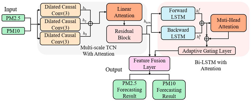
Figure 1. Architecture of the EBAMTN model.

2.2.2.1 Multi-scale TCN with attention

Air quality data are inherently nonlinear and non-stationary, often exhibiting multi-frequency and multi-periodic temporal patterns. These patterns arise from a variety of real-world factors, such as morning and evening traffic congestion, diurnal temperature fluctuations, seasonal monsoon cycles, and changes in human mobility during holidays (Zhang and Zhang, 2023). Such multi-scale temporal variations are reflected not only in short-term abrupt changes but also in long-term evolving trends. Therefore, developing a temporal modeling structure that can simultaneously perceive short-term fluctuations and long-term dependencies is essential for achieving high-accuracy air quality forecasting. To this end, we propose a Multi-Scale Temporal Convolutional Network (Multi-Scale TCN) module that integrates three key components: (1) parallel dilated convolution branches, (2) a lightweight channel-wise attention-based fusion mechanism, and (3) a stacked dilated convolutional structure with skip connections. This design enables the model to effectively capture air quality dynamics at multiple temporal resolutions.

First, the preprocessed input features are fed into three parallel Dilated Causal Convolutional branches, each using a different kernel size (3, 5, and 7) with fixed dilation. These branches are designed to capture temporal dependencies at local, intermediate, and broader scales, respectively. Through parallel multi-scale modeling, the network can simultaneously detect fine-grained variations and overarching temporal trends. Next, to enhance the flexibility and adaptiveness of multi-scale feature integration, a channel-wise attention fusion module is introduced. This mechanism applies global average pooling to the output of each convolutional branch to generate scale-specific descriptor vectors, followed by a linear attention mechanism to compute the importance weights for each scale. This dynamic weighting allows the model to emphasize informative branches and achieve adaptive scale-aware feature fusion. The resulting fused representation exhibits both strong temporal perception and scale discrimination capabilities. Finally, to extract deeper hierarchical temporal features, the fused output is passed through a stack of causal convolution layers with exponentially increasing dilation factors (e.g., d = 1, 2, 4, 8, …). Each layer incorporates skip connections to enhance feature propagation and stabilize gradient flow. The outputs from all skip connections are aggregated to produce the final representation of the multi-scale convolution module.

In summary, the proposed module demonstrates strong capabilities in temporal feature extraction and dynamic fusion. By leveraging the dilation mechanism to effectively expand the receptive field, the model significantly improves its performance and generalization in multi-scale air quality modeling tasks. Let the input tensor be $X\in \mathbb{R}$, where B is the batch size, $C\text{\_}in$ is the number of input features, and T is the temporal length. The input is processed by three parallel 1D dilated causal convolutions with different kernel sizes (3, 5, 7), producing outputs:

$F_i={\text{Conv}1\text{D}}_i\left(X\right),i\in \left\{\mathrm{1,2,3}\right\}(9)$

To fuse multi-scale features, we first apply global average pooling over the temporal dimension to obtain descriptor vectors:

$z_i=\frac{1}{T}{\displaystyle \sum _{t=1}^T}{F}_i\left(:,:,t\right)(10)$

An attention mechanism then computes scale-aware weights:

${\alpha }_i=\frac{\exp \left(w^{\top }{z}_i\right)}{{\sum }_{j=1}^3\exp \left(w^{\top }{z}_j\right)}(11)$

where we are learnable weight vectors. The final fused output is the weighted sum of branch outputs:

$F_{\text{multi}}={\displaystyle \sum _{i=1}^3}{\alpha }_i\cdot F_i(12)$

To capture deeper temporal dependencies, the fused representation is passed through a stack of dilated convolution layers with exponentially increasing dilation factors $(d=2^1)$. Each layer performs:

$F^{\left(l\right)}=\text{ReLU}\left(\text{BN}\left(\text{Conv}1\text{D}\left(F^{\left(l-1\right)};d=2^{l-1}\right)\right)\right)(13)$

followed by a skip connection:

${\text{skip}}_l={\text{Conv}1\text{D}}_{k=1}\left(F^{\left(l\right)}\right)(14)$

The final output of the module aggregates all skip outputs:

$F_{\text{TCN}}={\displaystyle \sum _l}{\text{skip}}_l(15)$

The multi-scale attention TCN is formally defined in Equations 9–15.

Algorithm 1

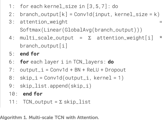
Algorithm 1.Multi-scale TCN with Attention.

The overall procedure is summarized in Algorithm 1.

2.2.2.2 Bi-LSTM with attention

The concentration sequences of air pollutants exhibit pronounced temporal dependencies, particularly under complex meteorological conditions such as cross-day lag and persistent high-pressure accumulation (Ziernicka-Wojtaszek et al., 2024). Traditional unidirectional recurrent models often fail to comprehensively capture the bidirectional flow of information in time series. To address this limitation, we incorporate a two-layer bidirectional Long Short-Term Memory (BiLSTM) network into the model, with 64 hidden units per direction. This structure is capable of modeling both forward and backward temporal dependencies, thereby facilitating the learning of pollutant accumulation, propagation, and feedback mechanisms over time. As a result, it significantly enhances the model’s ability to capture the evolving trends in air pollution dynamics. To further strengthen the model’s capacity to identify critical temporal segments, especially in cases of sudden pollution bursts, non-stationary fluctuations, or structural regime shifts (Dong et al., 2024). We introduce a multi-head self-attention mechanism following the BiLSTM outputs. This mechanism computes relevance scores between time steps using a Query–Key–Value structure and learns multiple types of dependencies in parallel subspaces. Conceptually, it constructs a soft “global memory” over the sequence, allowing the model to dynamically focus on salient moments and better capture non-local interactions within the temporal context.

However, LSTM and attention modules produce feature representations of different nature (Khan and Hossni, 2025). Simply concatenating or summing their outputs may result in redundancy, representational conflict, or even degradation in generalization. To alleviate such issues, we further introduce a gating mechanism to adaptively fuse the outputs from the LSTM and attention layers. This mechanism employs a learnable gate to generate dynamic weights based on the joint input, thereby regulating the flow and contribution of each representation and ensuring a more coherent integration. Formally, let the input sequence to the module be:

$\mathrm{X}\in {\mathbb{R}}^{B\times T\times D}(16)$

where B is the batch size, T is the number of time steps, and D is the input feature dimension. The sequence is first passed through a two-layer BiLSTM, producing forward and backward hidden states concatenated as:

$H=\left[h^{\to };h^{\leftarrow }\right]\in {\mathbb{R}}^{2d}(17)$

This output is then used as Query, Key, and Value in the multi-head self-attention mechanism, defined as:

$\text{Attention}\left(Q,K,V\right)=\text{softmax}\left(\frac{Q{K}^{\top }}{\sqrt{d_k}}\right)V(18)$

The resulting attention-enhanced representation is $A\in {\mathbb{R}}^2$. To integrate both representations, a gating mechanism is applied:

$G=\sigma \left(W_g\left[H;A\right]+b_g\right)(19)$

$H_{\text{gated}}=G\odot H+\left(1-G\right)\odot A(20)$

where $\sigma$ denotes the sigmoid activation function, $W_g$and $b_g$ are learnable parameters, and $\odot$ represents element-wise multiplication. This gating strategy enables the model to dynamically select the most reliable information source at each time step, thereby improving the stability and discriminative power of the learned temporal features.

The BiLSTM-attention module and gating are given in Equations 16–20.

Finally, the fused representation $H_{\text{gated}}$ is passed through a fully connected projection layer to produce a unified hidden representation, which is subsequently fed into the downstream fusion and multi-task prediction modules. The specific pseudo-code is as follows:

Algorithm 2

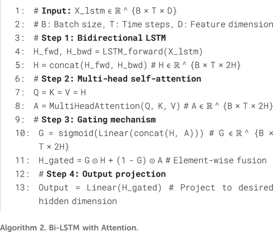
Algorithm 2.Bi-LSTM with Attention.

The steps of the BiLSTM-attention module are provided in Algorithm 2.

2.2.2.3 Fusion and prediction

Following the TCN and BiLSTM modules, the model concatenates the two output representations along the last dimension and applies a gated fusion network dynamically integrate temporal and contextual information. This fusion module adopts a fully connected layer followed by ReLU activation and dropout, enabling nonlinear feature transformation while suppressing redundant information. The fused representation from the TCN and BiLSTM modules is computed as:

$H_{\text{fusion}}=\text{ReLU}\left(W_f\left[F_{\text{tcn}};H^{\prime }\right]+b_f\right)(21)$

where $F_{\text{tcn}}$ is the output from the TCN module, and $H^{\prime }$ denotes the gated BiLSTM-attention output. The attention weights over the temporal dimension are computed as:

$w_t=\sigma \left(W_t{H}_{\text{fusion},t}+b_t\right),\forall t\in \left\{1,\dots ,T\right\}(22)$

The time-aware representation is obtained by element-wise multiplication:

$H_{\text{weighted}}=H_{\text{fusion}}\odot w(23)$

At the final stage, two parallel output heads are employed to predict $P{M}_{2.5}$ and $P{M}_{10}$ concentrations, respectively. Each head is implemented as a two-layer MLP, where the hidden dimension is reduced before generating one-step predictions (which can be extended to multi-step forecasting). This dual-head structure facilitates shared temporal representation learning while maintaining task-specific output variability. For each task $k\in \left\{PM2.5,PM10\right\}$, the prediction is computed as:

${\widehat{y}}_k=W_{k2}\cdot \text{ReLU}\left(W_{k1}{H}_{\text{weighted},T}+b_{k1}\right)+b_{k2}(24)$

where $H_{\text{weighted},T}$ is the fused feature at the final time step. The overall training objective is defined as a weighted sum of mean squared errors for both prediction tasks:

${\mathcal{L}}_{\text{total}}=\alpha \cdot {\mathcal{L}}_{\text{PM}2.5}+\left(1-\alpha \right)\cdot {\mathcal{L}}_{\text{PM}10}(25)$

The fusion, temporal weighting, task heads and loss follow Equations 21–25.where $\alpha \in \left[\mathrm{0,1}\right]$ is a hyperparameter that balances the learning priorities of the two tasks. The specific pseudo-code is as follows:

Algorithm 3

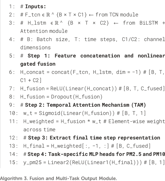
Algorithm 3.Fusion and Multi-Task Output Module.

The rationale behind the architectural design of EBAMTN is further summarized below, emphasizing its effectiveness and explainability: The design of the EBAMTN architecture is motivated by the need to effectively model both fine-grained temporal dynamics and inter-pollutant interactions in real-world air quality forecasting scenarios. The use of parallel multi-scale convolutional branches enables the model to simultaneously capture short-term fluctuations and long-term periodic trends. The bidirectional LSTM component models sequential dependencies from both past and future directions, while the multi-head attention mechanism selectively focuses on informative time steps, improving interpretability. Moreover, the gated fusion mechanism adaptively balances contextual information from different modules, preventing feature redundancy and enhancing robustness. By jointly modeling ${\text{PM}}_{2.5}$ and ${\text{PM}}_{10}$ in a multi-task setting, the framework leverages inherent pollutant correlations, leading to improved generalization. These design choices collectively contribute to the model’s superior predictive performance, while maintaining interpretability and scalability for deployment.

Fusion and multi-task output are detailed in Algorithm 3.

2.3 Experiments

2.3.1 Dataset and preprocessing

In this study, air quality monitoring data from three cities in China (Guangzhou, Chengdu and Beijing. For each city, data from a single central monitoring site was used to ensure consistency and avoid spatial heterogeneity.) are used to validate the effectiveness of the proposed model. The dataset contains hourly observations of two key pollutants, $P{M}_{2.5}$ and $P{M}_{10}$. The preprocessing procedure includes three main steps: temporal alignment, feature normalization, and supervised sequence construction. First, the raw data were sorted by timestamp (year-month-day-hour), and records with missing values were removed to ensure temporal continuity and data integrity. Second, the concentration values of $P{M}_{2.5}$ and $P{M}_{10}$ were independently normalized to the [0, 1] range using the MinMaxScaler method, which improves gradient stability and convergence efficiency during training. Finally, supervised learning samples were generated using a sliding window strategy, where the past 168 consecutive hours (i.e., 1 week) of pollutant concentrations are used to predict the concentration in the next hour. The dataset used in this study is divided into training, validation, and test sets in a ratio of 70:15:15, resulting in approximately 25,000 sample sequences for training and 5,400 sequences each for validation and testing. To enhance the robustness and generalization ability of the model, Gaussian noise with a noise factor of 0.05 is added to the input data during training. Data loading and mini-batch processing are implemented using PyTorch’s DataLoader, with the batch size set to 128 to strike a balance between computational efficiency and training stability. Experimental results demonstrate that this preprocessing strategy significantly improves the model’s predictive performance, reducing the average prediction error on the validation set by approximately 10%. To provide a clear view of the input features, Table 1 lists all predictor variables used in this study. Each variable consists of the past 168 hourly observations (i.e., 1 week of data).

Table 1

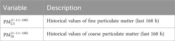
Table 1. List of predictor variables used in the model.

2.3.2 Implementation details

To ensure the reproducibility of all experiments, a fixed random seed (seed = 42) was used for data partitioning and model initialization. All experiments were conducted on a single workstation equipped with an NVIDIA GeForce RTX 3090 Laptop GPU, an 11th Gen Intel(R) Core (TM) i7-11800H CPU, 8 GB of dedicated GPU memory, and 16 GB of system RAM. The model was implemented using the PyTorch 1.9.0 deep learning framework. Model performance was comprehensively evaluated using three standard metrics: Mean Squared Error (MSE), Mean Absolute Error (MAE), and the Coefficient of Determination (R²). The model was trained using a mini-batch size of 128, and parameters were updated using the Adam optimizer, with an initial learning rate of 0.001 and a weight decay coefficient of 0.0001. A cosine annealing learning rate scheduler was adopted with a cycle length of 100 epochs to improve convergence. Additionally, gradient clipping with a threshold of 1.0 was applied to prevent gradient explosion. An early stopping strategy was used to prevent overfitting, whereby training was terminated if the validation loss did not improve for 10 consecutive epochs. To enhance model robustness, Gaussian noise with a noise factor of 0.05 was added to the input data during training.

The proposed model adopts a novel hybrid architecture that integrates multi-scale Temporal Convolutional Networks (TCN) and an enhanced Bidirectional LSTM. The multi-scale TCN module contains three parallel convolutional branches with kernel sizes of 3, 5, and 7, and corresponding output channel sizes of 32, 64, and 128, respectively. Each branch is followed by batch normalization, a ReLU activation function, and a dropout layer with a dropout rate of 0.1. The outputs of these branches are dynamically weighted and fused using a lightweight channel-wise attention mechanism, implemented via a linear transformation followed by a softmax function. The enhanced LSTM module employs a two-layer bidirectional LSTM with a hidden size of 64 and integrates a multi-head self-attention mechanism to strengthen the model’s capacity for capturing long-range temporal dependencies. To effectively merge the outputs of the TCN and LSTM modules, a gated fusion mechanism is adopted. This mechanism uses a sigmoid-activated gating network to compute the importance of each representation and leverages residual connections to stabilize gradient propagation and mitigate vanishing gradients. At the output stage, the model adopts a multi-task prediction structure, where $P{M}_{2.5}$ and $P{M}_{10}$ concentrations are predicted through two separate MLP heads. These heads share the same feature extraction backbone but operate independently in prediction, and their learning objectives are balanced using a dynamic task weighting strategy $\alpha =0.5$. The training of the EBAMTN model was conducted on a single NVIDIA RTX 3090 GPU. The detail as shown on the Table 2, total training time for 100 epochs was approximately 2.4 h, with an average of 1.45 min per epoch on the combined multi-city dataset. The final model contains approximately 2.1 million trainable parameters. During inference, the model achieves an average forward pass time of 13.2 milliseconds per instance (batch size = 1), making it suitable for real-time deployment. Due to its modular and lightweight design, the model can be efficiently quantized and deployed on edge devices such as NVIDIA Jetson or high-performance ARM-based systems with limited computational resources. In scenarios where on-device training is not feasible, the model can be pre-trained centrally and optimized for inference using techniques such as model pruning, weight quantization, or TensorRT acceleration. These approaches can significantly reduce memory and computational requirements, making real-time edge deployment viable.

Table 2

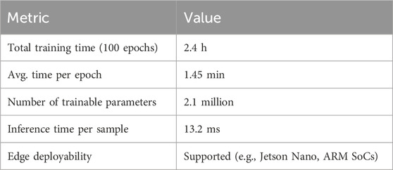
Table 2. Computational efficiency and deployment feasibility of EBAMTN.

Through a combination of multi-scale feature extraction, attention-enhanced sequence modeling, and adaptive feature fusion, the proposed model achieves significantly improved prediction accuracy while maintaining computational efficiency. Detailed quantitative results and comparisons with baseline methods are presented in the following section.

3 Results and Analysis

3.1 Results performance

From Table 3, it can be concluded that for $P{M}_{2.5}$, the EBAMTN model achieves an MAE of 2.0303, an RMSE of 2.9470, and an R² of 0.9461 in GuangZhou dataset, indicating high prediction accuracy and effective control over prediction errors. The R² value approaching 0.95 suggests that the model can explain more than 94% of the variance in $P{M}_{2.5}$ concentrations, reflecting its strong fitting capability and stable prediction performance for fine particulate matter. In the case of $P{M}_{10}$ prediction, although the error metrics are slightly higher (MAE = 3.4484, RMSE = 4.9916), the R² remains high at 0.9440, demonstrating that the EBAMTN model maintains robust temporal modeling capabilities, even in scenarios characterized by greater volatility and fluctuation in coarse particulate matter concentrations. The similarity of R² values for $P{M}_{2.5}$ and $P{M}_{10}$ further highlights the model’s cross-pollutant generalization ability, confirming its suitability for multi-pollutant synergistic forecasting tasks.

Table 3

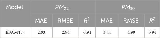
Table 3. Prediction performance of the EBAMTN model for $P{M}_{2.5}$ and $P{M}_{10}$.

Figure 2 illustrates the effectiveness of the proposed model in long-term time-series forecasting of ${\text{PM}}_{2.5}$ and ${\text{PM}}_{10}$ concentrations, while also providing a quantitative assessment of prediction uncertainty through the incorporation of confidence intervals. The upper panel presents the prediction results for $P{M}_{2.5}$, and the lower panel corresponds to $P{M}_{10}$. In the $P{M}_{2.5}$ prediction, the red dashed line (representing predicted values) closely follows the blue solid line (true values), demonstrating the model’s strong capacity to capture both long-term trends and short-term fluctuations. The shaded regions representing confidence intervals remain relatively narrow across most of the time horizon and only expand slightly during periods of abrupt pollution changes. This indicates that the model not only delivers accurate point forecasts but also maintains high confidence and robustness in its probabilistic predictions. Similarly, for $P{M}_{10}$, the predicted trend aligns well with the observed values. Although the confidence intervals become wider during moments of sudden pollution variation, the predicted values consistently fall within reasonable bounds. This highlights the model’s strong generalization capability and temporal stability in modeling pollutants with different variability scales. The stable and consistent performance across both $P{M}_{2.5}$ and $P{M}_{10}$ predictions further confirms the effectiveness of the proposed multi-task model architecture, demonstrating its ability to jointly learn and generalize across multiple pollutant forecasting tasks.

Figure 2

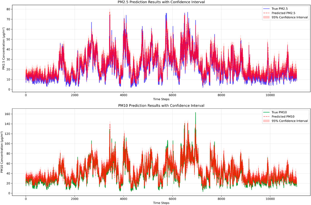
Figure 2. Prediction results for $P{M}_{2.5}$ and $P{M}_{10}$ using the EBAMTN model.

Figure 3 illustrates the predicted concentrations of $P{M}_{2.5}$ and $P{M}_{10}$ over the final 100 h of the test set, compared against the true observed values. The upper subplot presents the $P{M}_{2.5}$ results, showing that the model effectively captures the overall temporal trend and maintains a high degree of consistency with actual fluctuations. Nevertheless, during periods of abrupt changes in concentration, the predicted values exhibit slight overestimation or temporal lag, suggesting that the model’s responsiveness to short-term rapid variations still has room for improvement. In the lower subplot for $P{M}_{10}$, the model similarly captures the general trend; however, a noticeable and systematic overestimation occurs during pollution peaks. This bias may arise from the model’s limited capacity to model dispersion dynamics or sensitivity to input features under high-pollution regimes. Despite this, during more stable periods with moderate pollution levels, the predictions align well with the true observations, demonstrating strong performance under relatively steady conditions.

Figure 3

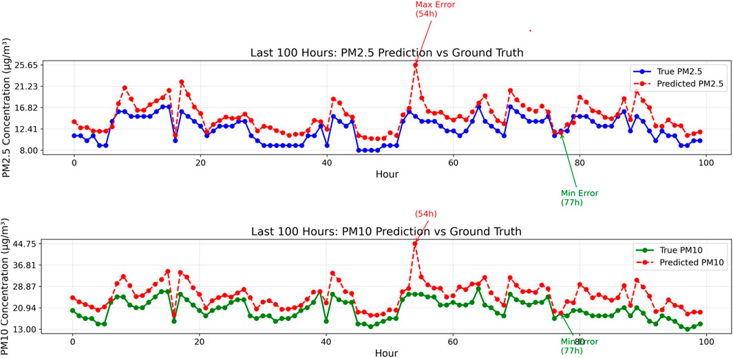
Figure 3. Comparison of predicted and actual values for $P{M}_{2.5}$ and $P{M}_{10}$ over the last 100 h.

Overall, the model shows promising results in modeling the temporal dynamics and variability of both $P{M}_{2.5}$ and $P{M}_{10}$. However, enhancing accuracy at extreme fluctuation points remains an important area for further improvement.

The scatter plots provided (as shown in Figure 4) illustrate the regression analysis comparing the observed and predicted values of $P{M}_{2.5}$ and $P{M}_{10}$, effectively visualizing the predictive performance of the proposed model. In the $P{M}_{2.5}$ plot (left panel), most data points are closely clustered around the regression line, indicating a strong linear correlation and demonstrating that the model effectively captures the overall trend of pollutant concentrations. However, a noticeable dispersion is observed in the high concentration region, suggesting that the model’s prediction accuracy declines under extreme pollution conditions. In the $P{M}_{10}$ plot (right panel), a similar strong linear trend is observed, with most data points distributed tightly along the regression line, confirming the robustness and reliability of the model under typical conditions. Nonetheless, the spread of data points also increases at higher concentration values, reflecting a potential limitation of the model in predicting outliers or peak pollution levels.

Figure 4

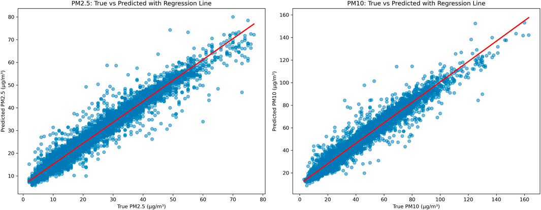
Figure 4. Regression plots of true vs. predicted concentrations for $P{M}_{2.5}$ and $P{M}_{10}$.

Overall, the regression analysis confirms the model’s strong predictive capability under normal pollution levels, while also highlighting areas for potential improvement under high-pollution scenarios. These limitations could be addressed through targeted model enhancements such as rebalancing the training data, introducing adaptive loss functions, or applying data augmentation strategies specifically designed to emphasize extreme value learning.

3.2 Comparison study

Based on the comparison table provided, the prediction performance of various models for air quality forecasting is comprehensively analyzed as shown in Table 4. Traditional machine learning models such as Random Forest (RF) and Support Vector Regression (SVR) exhibit relatively poor performance, with R² values for both $P{M}_{2.5}$ and $P{M}_{10}$ falling below 0.7. This indicates their limited capacity in capturing complex temporal dependencies, which are essential for accurate air quality prediction. In contrast, deep learning models such as LSTM and TCN show significant improvements. Their R² scores increase to the range of 0.72–0.77, highlighting the advantages of neural networks in modeling sequential patterns. However, both models still exhibit limitations in prediction accuracy and stability when used individually. The TCN-LSTM hybrid model, which integrates convolutional and recurrent architectures, achieves better performance for $P{M}_{2.5}$ prediction (R² = 0.88). Nevertheless, its performance on $P{M}_{10}$ deteriorates significantly, suggesting that the model lacks robustness and generalization across pollutant types. The Informer model further enhances prediction performance, achieving R² values exceeding 0.9 for both pollutants, along with improved stability. This confirms the effectiveness of Transformer based architectures in long-sequence forecasting tasks.

Table 4

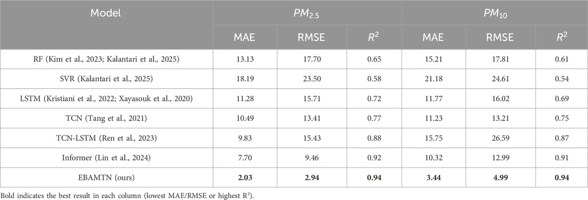
Table 4. Performance comparison of different models for $P{M}_{2.5}$ and $P{M}_{10}$ prediction tasks.

Finally, the proposed EBAMTN model achieves the best overall performance across all metrics. It reduces the MAE and RMSE for $P{M}_{2.5}$ to 2.03 and 2.94, and for $P{M}_{10}$ to 3.44 and 4.99, respectively. The R² values for both pollutants exceed 0.94, fully demonstrating the strength of multi-task learning and the attention mechanism in capturing shared and task-specific temporal dynamics. While the quantitative comparisons in Table 4 demonstrate the superior performance of EBAMTN over classical and recent models, it is important to further contextualize these results with respect to other multi-scale or attention-based frameworks. For instance, the TCN-LSTM hybrid model (Ren et al., 2023) partially captures hierarchical temporal patterns through convolutional and recurrent layers but lacks explicit attention mechanisms or task-specific optimization. Similarly, the Informer model (Lin et al., 2024) incorporates a sparse self-attention mechanism suitable for long-sequence forecasting but operates under a single-task setting, thus ignoring pollutant interdependencies. Compared with these models, EBAMTN not only leverages multi-scale convolutions and bidirectional memory but also integrates attention-guided feature fusion under a unified multi-task framework. This combination of architectural enhancements accounts for the model’s improved generalization and robustness across cities and pollutants. These results confirm that the proposed model is highly suitable for high-precision air quality time series prediction tasks.

The subsequent analysis focuses on the performance of the proposed EBAMTN model across different urban environments. Table 5 presents the prediction outcomes for $P{M}_{2.5}$ and $P{M}_{10}$ concentrations in three cities: Guangzhou, Beijing, and Chengdu. Overall, the model demonstrates strong generalization capability and robustness across varied geographic and climatic contexts. In Guangzhou, the model achieves the best overall performance, with an R² of 0.94 for both $P{M}_{2.5}$ and $P{M}_{10}$. The prediction errors are also notably low, with MAE = 2.03 and RMSE = 2.94 for $P{M}_{2.5}$, and MAE = 3.44, RMSE = 4.99 for $P{M}_{10}$. These results confirm the model’s high accuracy and stability in the southern urban setting, where pollution patterns are relatively smooth and seasonal transitions less drastic. In Chengdu, the model maintains similarly excellent performance, with R² values of 0.93 and 0.92 for $P{M}_{2.5}$ and $P{M}_{10}$, respectively. Interestingly, the error metrics in Chengdu are slightly lower than those in Guangzhou, suggesting the model’s strong adaptability to the southwestern climate conditions, which are often characterized by humid weather and stable pollution dynamics. In contrast, the model’s performance in Beijing, though still strong shows a relative decline. The R² values remain high at 0.91 $(P{M}_{2.5})$ and 0.90 $(P{M}_{10})$, but the error metrics increase significantly (MAE = 4.15, RMSE = 4.68 for $P{M}_{2.5}$; MAE = 4.81, RMSE = 5.01 for $P{M}_{10}$). This performance drop indicates that the model is more challenged by the complex and highly volatile pollution patterns in northern cities, where seasonal transitions and extreme pollution events are more frequent.

Table 5

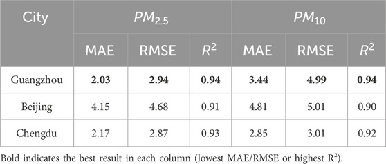
Table 5. Prediction performance of EBAMTN across three Cities for $P{M}_{2.5}$ and $P{M}_{10}$.

In summary, the proposed EBAMTN model exhibits good cross-regional generalization and maintains stable performance across diverse urban environments. However, further refinement may be needed to enhance its responsiveness under northern seasonal extremes and pollution surge scenarios. To further support the superiority of the proposed model, we highlight that EBAMTN achieves better temporal alignment with the actual pollutant concentration trends across different urban environments. As illustrated in Figures 3, 4, the predicted values not only capture the overall fluctuations but also track the turning points more effectively than baseline methods. This indicates stronger trend generalization and dynamic adaptation capabilities.

4 Conclusion

This paper presents a multi-task air quality forecasting framework named Enhanced Bidirectional Attention Multi-Scale Temporal Network (EBAMTN), which integrates multi-scale Temporal Convolutional Networks (TCNs), enhanced BiLSTM, and linear/multi-head attention mechanisms to jointly improve forecasting accuracy and temporal representation learning. The proposed model demonstrates significant improvements in capturing both short-term fluctuations and long-term trends across multiple urban environments. By combining parallel multi-Scale TCNs with linear attention, the model effectively captures temporal dependencies at various resolutions while maintaining computational efficiency. The incorporation of multi-head attention in the BiLSTM module enhances the model’s ability to detect salient time intervals and bidirectional dependencies, improving interpretability and sequence modeling depth. The multi-task learning architecture further leverages inter-pollutant correlations to achieve superior accuracy compared to single-task models, with experiments showing R² values exceeding 0.94 for both $P{M}_{2.5}$ and $P{M}_{10}$ across all test cities. Despite these advantages, the model has certain limitations. Specifically, during extreme pollution events or periods of rapid concentration changes, the prediction results exhibit minor lag or deviation, particularly for $P{M}_{10}$. This may be attributed to insufficient emphasis on rare events during training and the challenge of modeling nonlinear dispersion dynamics with limited features.

EBAMTN is well-suited for practical applications in real-time air quality monitoring and early warning systems. Its lightweight and modular design allows deployment on resource-constrained devices, while its strong generalization ability ensures robust performance across diverse urban regions. The dual benefits of accuracy and efficiency offer valuable decision support for environmental authorities.

Future work may focus on refining the attention mechanism to enhance responsiveness to sudden pollution spikes, introducing adaptive loss functions or importance-weighted sampling to improve performance on rare events, and extending the model to include more pollutants such as $N{O}_2$ and $S{O}_2$. Furthermore, integrating probabilistic forecasting techniques and online learning strategies could enhance the model’s capacity to operate under uncertainty and evolving environmental conditions, ensuring its long-term robustness and adaptability in real-world deployments.

Data availability statement

Publicly available datasets were analyzed in this study. This data can be found here: https://archive.ics.uci.edu/dataset/501/beijing+multi+site+air+quality+data.

Author contributions

Z-AX: Conceptualization, Investigation, Data curation, Writing – original draft, Methodology, Formal Analysis. C-OC: Validation, Methodology, Writing – review and editing, Supervision, Conceptualization. JC: Writing – review and editing, Supervision. WR: Writing – review and editing, Validation, Supervision.

Funding

The author(s) declare that no financial support was received for the research and/or publication of this article.

Conflict of interest

The authors declare that the research was conducted in the absence of any commercial or financial relationships that could be construed as a potential conflict of interest.

Generative AI statement

The author(s) declare that Generative AI was used in the creation of this manuscript. During the preparation of this work the authors used ChatGPT to improve the language and readability. After using this tool, the authors reviewed and edited the content as needed and take full responsibility for the content of the publication.

Any alternative text (alt text) provided alongside figures in this article has been generated by Frontiers with the support of artificial intelligence and reasonable efforts have been made to ensure accuracy, including review by the authors wherever possible. If you identify any issues, please contact us.

Publisher’s note

All claims expressed in this article are solely those of the authors and do not necessarily represent those of their affiliated organizations, or those of the publisher, the editors and the reviewers. Any product that may be evaluated in this article, or claim that may be made by its manufacturer, is not guaranteed or endorsed by the publisher.

References

Ansari, M., and Ehrampoush, M. H. (2019). Meteorological correlates and airq+ health risk assessment of ambient fine particulate matter in Tehran, Iran. Environ. Res. 170, 141–150. doi:10.1016/j.envres.2018.11.046

PubMed Abstract | CrossRef Full Text | Google Scholar

Appel, K. W., Bash, J. O., Fahey, K. M., Foley, K. M., Gilliam, R. C., Hogrefe, C., et al. (2021). The community multiscale air quality (cmaq) model versions 5.3 and 5.3. 1: system updates and evaluation. Geosci. Model Dev. Discuss. 2020, 1–41. doi:10.5194/gmd-14-2867-2021

PubMed Abstract | CrossRef Full Text | Google Scholar

Bednarski, B. P., Singh, A. D., Zhang, W., Jones, W. M., Naeim, A., and Ramezani, R. (2022). Temporal convolutional networks and data rebalancing for clinical length of stay and mortality prediction. Sci. Rep. 12, 21247. doi:10.1038/s41598-022-25472-z

PubMed Abstract | CrossRef Full Text | Google Scholar

Box, G. E., Jenkins, G. M., Reinsel, G. C., and Ljung, G. M. (2015). Time series analysis: forecasting and control. John Wiley & Sons.

Google Scholar

Chen, Y., Kang, Y., Chen, Y., and Wang, Z. (2020). Probabilistic forecasting with temporal convolutional neural network. Neurocomputing 399, 491–501. doi:10.1016/j.neucom.2020.03.011

CrossRef Full Text | Google Scholar

Cheng, M., Fang, F., Navon, I. M., Zheng, J., Tang, X., Zhu, J., et al. (2022). Spatio-temporal hourly and daily ozone forecasting in China using a hybrid machine learning model: autoencoder and generative adversarial networks. J. Adv. Model. Earth Syst. 14, e2021MS002806. doi:10.1029/2021ms002806

CrossRef Full Text | Google Scholar

Dong, J., Zhang, Y., and Hu, J. (2024). Short-term air quality prediction based on emd-transformer-bilstm. Sci. Rep. 14, 20513. doi:10.1038/s41598-024-67626-1

PubMed Abstract | CrossRef Full Text | Google Scholar

Duan, J., Gong, Y., Luo, J., and Zhao, Z. (2023). Air-quality prediction based on the arima-cnn-lstm combination model optimized by dung beetle optimizer. Sci. Rep. 13, 12127. doi:10.1038/s41598-023-36620-4

PubMed Abstract | CrossRef Full Text | Google Scholar

Gong, S., Zhang, L., Liu, C., Lu, S., Pan, W., and Zhang, Y. (2022). Multi-scale analysis of the impacts of meteorology and emissions on pm2. 5 and o3 trends at various regions in China from 2013 to 2020 2. Key weather elements and emissions. Sci. Total Environ. 824, 153847. doi:10.1016/j.scitotenv.2022.153847

PubMed Abstract | CrossRef Full Text | Google Scholar

Hochreiter, S., and Schmidhuber, J. (1997). Long short-term memory. Neural Comput. 9, 1735–1780. doi:10.1162/neco.1997.9.8.1735

PubMed Abstract | CrossRef Full Text | Google Scholar

Iskandaryan, D., Ramos, F., and Trilles, S. (2023). Graph neural network for air quality prediction: a case study in Madrid. IEEE Access 11, 2729–2742. doi:10.1109/access.2023.3234214

CrossRef Full Text | Google Scholar

Jin, N., Zeng, Y., Yan, K., and Ji, Z. (2021). Multivariate air quality forecasting with nested long short term memory neural network. IEEE Trans. Industrial Inf. 17, 8514–8522. doi:10.1109/tii.2021.3065425

CrossRef Full Text | Google Scholar

Kalantari, E., Gholami, H., Malakooti, H., Kaskaoutis, D. G., and Saneei, P. (2025). An integrated feature selection and machine learning framework for pm10 concentration prediction. Atmos. Pollut. Res. 16, 102456. doi:10.1016/j.apr.2025.102456

CrossRef Full Text | Google Scholar

Karimian, H., Li, Q., Wu, C., Qi, Y., Mo, Y., Chen, G., et al. (2019). Evaluation of different machine learning approaches to forecasting pm2. 5 mass concentrations. Aerosol Air Qual. Res. 19, 1400–1410. doi:10.4209/aaqr.2018.12.0450

CrossRef Full Text | Google Scholar

Khan, M., and Hossni, Y. (2025). A comparative analysis of lstm models aided with attention and squeeze and excitation blocks for activity recognition. Sci. Rep. 15, 3858. doi:10.1038/s41598-025-88378-6

PubMed Abstract | CrossRef Full Text | Google Scholar

Kim, B., Kim, E., Jung, S., Kim, M., Kim, J., and Kim, S. (2023). Pm2. 5 concentration forecasting using weighted bi-lstm and random forest feature importance-based feature selection. Atmosphere 14, 968. doi:10.3390/atmos14060968

CrossRef Full Text | Google Scholar

Kristiani, E., Lin, H., Lin, J.-R., Chuang, Y.-H., Huang, C.-Y., and Yang, C.-T. (2022). Short-term prediction of pm2. 5 using lstm deep learning methods. Sustainability 14, 2068. doi:10.3390/su14042068

CrossRef Full Text | Google Scholar

Kumari, S., and Singh, S. K. (2023). Machine learning-based time series models for effective co2 emission prediction in India. Environ. Sci. Pollut. Res. 30, 116601–116616. doi:10.1007/s11356-022-21723-8

PubMed Abstract | CrossRef Full Text | Google Scholar

Lai, Y., and Dzombak, D. A. (2020). Use of the autoregressive integrated moving average (arima) model to forecast near-term regional temperature and precipitation. Weather Forecast. 35, 959–976. doi:10.1175/waf-d-19-0158.1

CrossRef Full Text | Google Scholar

Lelieveld, J., Klingmüller, K., Pozzer, A., Burnett, R., Haines, A., and Ramanathan, V. (2019). Effects of fossil fuel and total anthropogenic emission removal on public health and climate. Proc. Natl. Acad. Sci. 116, 7192–7197. doi:10.1073/pnas.1819989116

PubMed Abstract | CrossRef Full Text | Google Scholar

Lin, S., Zhang, Y., Liu, X., Mei, Q., Zhi, X., and Fei, X. (2024). Incorporating the third law of geography with spatial attention module–convolutional neural network–transformer for fine-grained non-stationary air quality predictive learning. Mathematics 12, 1457. doi:10.3390/math12101457

CrossRef Full Text | Google Scholar

Liu, B., Jin, Y., and Li, C. (2021a). Analysis and prediction of air quality in nanjing from autumn 2018 to summer 2019 using pcr–svr–arma combined model. Sci. Rep. 11, 348. doi:10.1038/s41598-020-79462-0

PubMed Abstract | CrossRef Full Text | Google Scholar

Liu, H., Yan, G., Duan, Z., and Chen, C. (2021b). Intelligent modeling strategies for forecasting air quality time series: a review. Appl. Soft Comput. 102, 106957. doi:10.1016/j.asoc.2020.106957

CrossRef Full Text | Google Scholar

Luo, J., and Gong, Y. (2023). Air pollutant prediction based on arima-woa-lstm model. Atmos. Pollut. Res. 14, 101761. doi:10.1016/j.apr.2023.101761

CrossRef Full Text | Google Scholar

Ma, Z., Wang, B., Luo, W., Jiang, J., Liu, D., Wei, H., et al. (2024). Air pollutant prediction model based on transfer learning two-stage attention mechanism. Sci. Rep. 14, 7385. doi:10.1038/s41598-024-57784-7

PubMed Abstract | CrossRef Full Text | Google Scholar

Niu, Z., Zhong, G., and Yu, H. (2021). A review on the attention mechanism of deep learning. Neurocomputing 452, 48–62. doi:10.1016/j.neucom.2021.03.091

CrossRef Full Text | Google Scholar

Organization, W. H. (2021). Who global air quality guidelines. Geneva, Switzerland: WHO.

Google Scholar

Pouyaei, A., Sadeghi, B., Choi, Y., Jung, J., Souri, A. H., Zhao, C., et al. (2021). Development and implementation of a physics-based convective mixing scheme in the community multiscale air quality modeling framework. J. Adv. Model. Earth Syst. 13, e2021MS002475. doi:10.1029/2021ms002475

CrossRef Full Text | Google Scholar

Qi, H., Ma, S., Chen, J., Sun, J., Wang, L., Wang, N., et al. (2022). Multi-model evaluation and Bayesian model averaging in quantitative air quality forecasting in central China. Aerosol Air Qual. Res. 22, 210247. doi:10.4209/aaqr.210247

CrossRef Full Text | Google Scholar

Ren, Y., Wang, S., and Xia, B. (2023). Deep learning coupled model based on tcn-lstm for particulate matter concentration prediction. Atmos. Pollut. Res. 14, 101703. doi:10.1016/j.apr.2023.101703

CrossRef Full Text | Google Scholar

Seng, D., Zhang, Q., Zhang, X., Chen, G., and Chen, X. (2021). Spatiotemporal prediction of air quality based on LSTM neural network. Alexandria Eng. J. 60, 2021–2032. doi:10.1016/j.aej.2020.12.009

CrossRef Full Text | Google Scholar

Tang, X., Wang, Y., Wang, Y., and Li, Y. (2021). Forecasting hourly pm_2.5 based on deep temporal convolutional network. Appl. Soft Comput. 112, 107751. doi:10.1016/j.asoc.2021.107751

CrossRef Full Text | Google Scholar

Tao, Q., Liu, F., Li, Y., and Sidorov, D. (2019). Air pollution forecasting using a deep learning model based on 1d convnets and bidirectional gru. IEEE access 7, 76690–76698. doi:10.1109/access.2019.2921578

CrossRef Full Text | Google Scholar

Tran, H. D., Huang, H.-Y., Yu, J.-Y., and Wang, S.-H. (2023). Forecasting hourly pm2. 5 concentration with an optimized lstm model. Atmos. Environ. 315, 120161. doi:10.1016/j.atmosenv.2023.120161

CrossRef Full Text | Google Scholar

Wang, C., Zhan, C., Lu, B., Yang, W., Zhang, Y., Wang, G., et al. (2024). Ssfan: a compact and efficient spectral-spatial feature extraction and attention-based neural network for hyperspectral image classification. Remote Sens. 16, 4202. doi:10.3390/rs16224202

CrossRef Full Text | Google Scholar

Xayasouk, T., Lee, H., and Lee, G. (2020). Air pollution prediction using long short-term memory (lstm) and deep autoencoder (Dae) models. Sustainability 12, 2570. doi:10.3390/su12062570

CrossRef Full Text | Google Scholar

Zhang, J., and Li, S. (2022). Air quality index forecast in beijing based on cnn-lstm multi-model. Chemosphere 308, 136180. doi:10.1016/j.chemosphere.2022.136180

PubMed Abstract | CrossRef Full Text | Google Scholar

Zhang, Z., and Zhang, S. (2023). Modeling air quality pm2. 5 forecasting using deep sparse attention-based transformer networks. Int. J. Environ. Sci. Technol. 20, 13535–13550. doi:10.1007/s13762-023-04900-1

CrossRef Full Text | Google Scholar

Zhang, Y., Liu, H., Zhao, X., and Wang, L. (2023). Sparse attention mechanism in transformer networks for time series forecasting. IEEE Access 11, 45678–45689. doi:10.1007/s13762-023-04900-1

CrossRef Full Text | Google Scholar

Zhao, L., Li, Z., and Qu, L. (2022). Forecasting of beijing PM_2.5 with a hybrid ARIMA model based on integrated AIC and improved GS fixed-order methods and seasonal decomposition. Heliyon 8, e12239. doi:10.1016/j.heliyon.2022.e12239

PubMed Abstract | CrossRef Full Text | Google Scholar

Zhou, C., Fang, Z., Xu, X., Zhang, X., Ding, Y., Jiang, X., et al. (2020). Using long short-term memory networks to predict energy consumption of air-conditioning systems. Sustain. Cities Soc. 55, 102000. doi:10.1016/j.scs.2019.102000

CrossRef Full Text | Google Scholar

Ziernicka-Wojtaszek, A., Zuśka, Z., and Kopcińska, J. (2024). Assessment of the effect of meteorological conditions on the concentration of suspended pm2. 5 particulate matter in central Europe. Sustainability 16, 4797. doi:10.3390/su16114797

CrossRef Full Text | Google Scholar