Cumulative probability and regression analysis of ecosystem disruption by an integrated mechanism of AI with FF-flood dynamical model

Introduction: This article highlights the applications of artificial intelligence in the flood dynamics analysis with its effects on the ecosystem with the help of mathematical modeling and simulations.

Problem Statement: Flood prediction with control remains critical for all walks of lives. Due to nonlinear hydrological mechanism and delayed responses within natural systems, the integer-order models often fail to capture memory effects.

Results: A FF-Flood dynamical system is developed with five variables to capture the dynamics of flood more precisely. The theoretical results of the model ensure the existence of solution, uniqueness of solution, and stability analysis. Ecosystem disruption is inferred through dynamic water level changes, surface runoff and water contamination.

Methodology: A novel FF-Flood dynamical system is constructed which is integrating the surface storage, runoff, river flow, water level and flood area. Existence and boundedness are analytically verified with reference of fixed-point theory, and time-domain simulations demonstrate sensitivity patterns. The results are affirmed by the help of AI deep learning analysis: as process innovation.

1 Introduction

Climate change is a critical environmental complex challenge of the 21st century which is disrupting ecosystems, altering weather dynamics, and transforming human-environment interactions across the globe (Trenberth, 2014; Yang et al., 2014; Gazi et al., 2025). One of the most prominent outcomes of climate change is its disruptive impact on the natural hydrological system, leading to changes in rainfall systems, temperature rise, and an enhancement in extreme events like flooding. The hydrological system, which manages the natural exchange of water between the atmosphere, land, and underground sources, is increasingly disrupted by floods. Enhanced evaporation rates, irregular rainfall distribution, and unpredictable surface runoff and groundwater have magnified the frequency and severity of floods, damaging drainage networks and disturbing the ecological systems and human infrastructure (Wu et al., 2012; Nan et al., 2011; Barry et al., 2025). These climatic disruption have been induced by several sources. The consistent rise in global temperatures due to greenhouse gas emissions has triggered profound disruptions in the Earth’s climate system. The Intergovernmental Panel on Climate Change (IPCC) has warned that the average global temperature has increased by approximately $1.1^{\mathrm{deg}}C$ since the late 19th century. This warming trend has led to widespread results including the melting of polar ice, warming of ocean waters, and more frequent extreme heat events. These climatic transmission are also disrupting precipitation dynamics, resulting in more intense rainfall causing the floods while causing droughts in others for a long time (An et al., 2018; Cao et al., 2024; Amnuaylojaroen, 2023).

In the context of flooding, warmer air can retain greater moisture, significantly increasing the probability of heavy rainfall and storm-driven floods. Research indicates a consistent 2% rise per decade in annual precipitation across mid-latitude regions since the 1950s. Such patterns have resulted in devastating flood events-for instance, the catastrophic 2021 floods in Germany and Belgium, which inflicted over 40 billion in damages. Conversely, some regions face persistent water scarcity due to reduced snowpack, such as the southwestern United States, where the 2020–2022 megadrought marked the driest period in over a millennium (Janni et al., 2024; Ripple et al., 2024; Van Daalen et al., 2024).

These climatic changes place severe stress on water systems, agriculture, and disaster preparedness, amplifying the risks to human population and ecosystems together. The intersection of severe precipitation and outdated urban infrastructure often leads to overwhelmed drainage systems, urban floods, and loss of life and property. Addressing the threat of flood disasters necessitates urgent climate action-namely reducing emissions, enhancing resilient infrastructure, and implementing adaptive water governance. Sustained collaboration between scientists, policymakers, and communities is important to mitigating future impacts and ensuring resilience against worsening hydrological disruptions (Cai et al., 2024; Su and Ullah, 2024; Yaseen et al., 2024).

Floods are natural phenomenon that occur when water levels exceed the normal limits of rivers, lakes, or other water-bodies. The basic causes are including; heavy rainfall, rapid snowmelt, or dams failures. These events create a dynamic system where the balance between water volume, velocity, and the environment transfers dramatically (Wang et al., 2024; Rogers et al., 2025). The floods play dual role on ecosystems they are destructive for some regions while beneficial for others. On one hand, floods can disrupt habitats, affect wildlife, and cause soil erosion, causing to long-term biodiversity loss. On the other hand, floods also play a role in nutrient cycling by restructuring sediments and organic material, which can enhance soil fertility and improve the growth of plant species. The flood dynamic system is, therefore, a complex interaction between the natural forces and the resilience of the ecosystems it affects, highlighting the complex mechanism between environmental factors and the dependent organisms (Sun et al., 2024; Clarke et al., 2023; Badawy et al., 2024).

Floods are complex hydrological phenomenon influenced by a range of interacting natural and anthropogenic variables. Intense and/or prolonged rainfall, rapid snowmelt, topographic variations, and saturated soil factors often serve as basic natural flood resources (Salhi et al., 2024; Hamed et al., 2024; Darvishi Boloorani et al., 2024). Human activities such as urbanization, deforestation, and inadequate drainage mechanisms further implies flood risks by disrupting the natural flow and absorption of water. In flood dynamical systems, nonlinear feedback mechanisms between rainfall, runoff, river discharge, and land use jointly shape the intensity and duration of flooding dynaimcs (Gabr, 2023; Gebrael et al., 2024).

The repercussions of floods are far-reaching, extending beyond immediate property destruction. Financially, they cause significant costs on infrastructure repair, emergency response, and long-term economic recovery (Jonkman et al., 2024). Ecologically, floods can alter habitats, contaminate water, and lead to the transmission or death of wildlife. Prolonged overflow can also disrupt nutrient cycles and degrade agricultural land, dominating to food insecurity (Van Houtven, 2024; Terry et al., 2023). Therefore, the study of flood dynamical systems is important for developing predictive models and sustainability procedures to mitigate these downstream effects.

The Figure 1, highlights the floods and their financial and ecological impacts on Egypt, Algeria, Tunisia and Morocco. The evolution of flood-related financial and ecological impacts in Egypt, Algeria, Tunisia, and Morocco from 2015 to 2022. Financial losses are in million USD, showing a consistent growth in the graph in all countries. The Egypt is experiencing the most critical rise. Ecological loss, shown by a dimensionless index, also increases steadily, describing mounting environmental stress linked to recurrent flooding. Tunisia and Morocco have shown lower but gradually increasing impacts, whereas Algeria maintains a more moderate dynamics. This graph shows the growing effects of floods on both economic infrastructure and ecosystems across the MENA region, highlighting the need for significant flood management strategies (Gabr, 2023; Gebrael et al., 2024; Jonkman et al., 2024; Van Houtven, 2024; Terry et al., 2023; Kurniawan et al., 2024).

Figure 1

Figure 1. Subfigures present statistical data for the years 2015–2022: (a) financial impacts of floods (in million USD) and (b) ecological effects indices for Egypt, Algeria, Tunisia, and Morocco between 2015 and 2022.

1.1 Fractional order modeling of dynamical systems

Fractional differential equations (FDEs) suggest a pivotal extension of classical calculus. These are used to model systems with memory and hereditary aspects which make them more suitable for resilient real-world problems. In applied scientific field, FDEs have been successfully applied to viscoelastic materials, fluid dynamics, control theory, and biological problems. They capture anomalous diffusion and long-range temporal habits more precise than integer-order systems (Sabatier et al., 2007; Herrmann, 2011). Their viability gives accurate representations of dynamic intricate systems, especially where classical models are not well applicable (Caputo and Fabrizio, 2015; Bas et al., 2019). In the recent works, the readers can see a bridging role of FDEs between theoretical analysis and computational results in the works (Khan et al., 2025a; Khan et al., 2025b; Ahmad et al., 2024).

By incorporating fractal geometry into the idea of fractional derivatives, the fractal-fractional derivative is an expansion of the traditional fractional calculus. It simulates systems with long-range dependencies and irregular non-differentiable activities, which are prevalent of complex and natural phenomena. Fractal-fractional derivatives, in comparison to integer-order derivatives, are durable to capture anomalous diffusion and memory problems (Atangana, 2017; Atangana and Qureshi, 2019; Atangana and Araz, 2020). Due to these properties, they are applied in fields such as epidemiology for modeling of disease transmission including sophisticated time-dependent relationships. Additionally, they are used in biology, physics, and finance to explain phenomena like as anomalous diffusion, diffusion in porous media, and chaotic system behaviors, providing more realistic and realistic representations of dynamics in the real world. For more detail about the applications and usefulness of the fractional derivatives and their applications in the environmental sciences, we refer the readers to the works (Sekerci, 2020; Kha et al., 2024; Kumar et al., 2021) and the references therein.

Definition 1.1. Assume that ${\psi }^{⊛}(\mathfrak{t})$ is a fractal differentiable function in the interval $(a,b)$ of order $\varpi$, then the fractal fractional derivative of ${\psi }^{⊛}\mathfrak{t}$ of order $\vartheta \in (\mathrm{0,1})$ in the Caputo’s sense is: ${}^{FF}{}_0{D}_{\mathfrak{t}}^{\vartheta ,\varpi }{\psi }^{⊛}=\frac{\mathfrak{M}(\vartheta )}{1-\vartheta }{\int }_0^{\mathfrak{t}}\frac{d}{d{t}^{\varpi }}{E}_{g_1^{⊛}}\left(-\frac{\vartheta }{1-\vartheta }{(\mathfrak{t}-s)}^{\vartheta }\right){\psi }^{⊛}(s)ds$, where $\mathfrak{M}(\vartheta )=1-\vartheta +\frac{\vartheta }{\mathrm{\Gamma }\vartheta }$.

Definition 1.2. Assume that ${\psi }^{⊛}$ is continues function (a, b) then the fractal-fractional integral of ${\psi }^{⊛}$ of order $\vartheta$ having Mittag–Leffler type kernal is given by ${}^{FF}{}_0{I}_{\mathfrak{t}}^{\vartheta ,\varpi }{\psi }^{⊛}=\frac{\vartheta \varpi }{\mathfrak{M}(\vartheta )\mathrm{\Gamma }\vartheta }{\int }_0^{\mathfrak{t}}{s}^{\varpi -1}{\psi }^{⊛}(s){(\mathfrak{t}-s)}^{\vartheta -1}ds+\frac{\varpi (1-\vartheta ){\mathfrak{t}}^{(\varpi -1)}}{\mathfrak{M}(\vartheta )}{\psi }^{⊛}$.

In the onward expressions, we will use $\mathcal{H}(\mathfrak{t},s)=s^{\varpi -1}{(\mathfrak{t}-s)}^{\vartheta -1}$, for simplicity. We introduce a Banach space of $\mathcal{B}=\{u\in C([0,T]:\mathbb{R})\}$, with a norm $\Vert u\Vert ={\max }_{\mathfrak{t}\in [0,T]}|u(\mathfrak{t})|$.

1.2 AI applications in science

Artificial Intelligence (AI) plays a vital role in analyzing systems by offering advanced techniques for modeling, forecasting, and optimization. In scenarios where system variables change over time, such as in dynamic environments, AI techniques including machine learning and neural networks efficiently handles at managing intricate and nonlinear patterns that conventional statistical methods often try to capture (Kumar and Mani, 1994; Böttcher et al., 2022). Artificial Intelligence (AI) plays a pivotal role in uncovering patterns from large datasets, capturing dynamical behaviors, and developing real-time forecasts. Techniques such as Recurrent Neural Networks (RNNs) and Long Short-Term Memory (LSTM) models are extensively applied for analyzing time-series data and anomalies recognitions. Additionally, AI contributes to solving inverse problems by finding system parameters from observed data. These methods also support automated model selection, parameter tuning, and error analysis, thereby enhancing the precision of dynamic simulations. Consequently, AI-driven approaches are increasingly adopted in domains like climate analysis, economic prediction, and engineering systems, where modeling complex and evolving phenomena is essential (Yuksel, 2024; Sharma et al., 2025; Khan et al., 2025c; Khan et al., 2025d).

1.2.1 FF-mathematical modeling of flood dynamical system

The dynamics of the presumed model is based on the excessive rainfall aiding to the flood demonstrated in the Figure 2. The excessive rainfall is raising to the water level in the rivers which are causing to the soil erosion and disrupting the natural water cycle which in severe cases causing to the floods. In this work, we assume the following as models’ variables; surface storage $(\mathfrak{S})$, surface runoff $({\mathfrak{Q}}_s)$, river flow $({\mathfrak{Q}}_r)$, water level $(\mathcal{H})$, and the area affected by flooding $({\mathfrak{A}}_f)$. The model is composed of ordinary differential equations (ODEs), modulated by a time-varying rainfall input $\mathfrak{R}(t)$, which is taken as a periodic function:

$\mathfrak{R}\left(t\right)=5\sin \left(0.2t\right)+10.$

Figure 2

Figure 2. Excessive rain fall raising to the water levels in rivers causing to the runoff of land structures and resulting to the floods and catastrophic situations.

Let $\mathbf{y}(t)={[\mathfrak{S}(t),{\mathfrak{Q}}_s(t),{\mathfrak{Q}}_r(t),\mathcal{H}(t),{\mathfrak{A}}_f(t)]}^{\top }$. The model is considered in the fractal-fractional sense of derivative:

$\left\{\begin{array}{cc}{}^{FF}{}_0{D}_{\mathfrak{t}}^{\vartheta ,\varpi }\mathfrak{S}\hfill & =f_1\mathfrak{R}\left(t\right)-f_2\mathfrak{S}-I,\hfill \\ {}^{FF}{}_0{D}_{\mathfrak{t}}^{\vartheta ,\varpi }{\mathfrak{Q}}_s\hfill & =\eta \max \left(\mathfrak{R}\left(t\right)-\theta \mathfrak{S}-I,0\right)-\mu {\mathfrak{Q}}_s,\hfill \\ {}^{FF}{}_0{D}_{\mathfrak{t}}^{\vartheta ,\varpi }{\mathfrak{Q}}_r\hfill & =\lambda {\mathfrak{Q}}_s-\delta {\mathfrak{Q}}_r,\hfill \\ {}^{FF}{}_0{D}_{\mathfrak{t}}^{\vartheta ,\varpi }\mathcal{H}\hfill & =\varphi \max \left({\mathfrak{Q}}_r-{\mathfrak{Q}}_{\text{cap}},0\right)-\zeta \mathcal{H},\hfill \\ {}^{FF}{}_0{D}_{\mathfrak{t}}^{\vartheta ,\varpi }{\mathfrak{A}}_f\hfill & =\rho \mathcal{H}-\gamma {\mathfrak{A}}_f,\hfill \end{array}\right.$

where $\mathfrak{I}$ denotes the infiltration rate, expressed as:

$\mathfrak{I}=k_i\max \left(\mathfrak{S}-{\mathfrak{S}}_{\text{sat}},0\right).$

Each term models physical processes relevant to flood behavior:

$•$ $\mathfrak{S}$: collects rain and loses water through runoff and infiltration.

$•$ ${\mathfrak{Q}}_s$: increases with excess rainfall and decreases through drainage.

$•$ ${\mathfrak{Q}}_r$: river flow builds up from surface runoff and decays naturally.

$•$ $\mathcal{H}$: rises when river flow exceeds capacity, decreases via dissipation.

$•$ ${\mathfrak{A}}_f$: flood extent grows with rising water level and recedes over time. The numerical values of the parameters are given in the Table 1.

Table 1

Table 1. Parameter definitions and values used in the FF-Flood dynamical system (1.1).

1.4 Novelty statement

$•$ Novelty: An FF-Flood dynamical system is developed incorporating memory effects and nonlinear interactions, capturing delayed hydrological aids often missed by classical differential equations.

$•$ Significance: The model explores how parameter shifts in infiltration and runoff significantly influence flood extent and timing, offering improved understanding of ecosystem disruptions.

$•$ Applicability: This model can predict water level raise in the rivers aiding to the floods, planning, and risk management by simulating different features under different environmental and climatic situations.

2 Mathematical analysis of the model

With the help of fixed point procedure, we check the existence of FF-Flood model (1.1). For this, we apply the FF-integral on the system (1.1) and get

$\left\{\begin{array}{cc}\mathfrak{S}\left(\mathfrak{t}\right)-\mathfrak{S}\left(0\right)\hfill & =\frac{\vartheta \varpi }{\mathfrak{M}\left(\vartheta \right)\mathrm{\Gamma }\vartheta }{\int }_0^{\mathfrak{t}}\mathcal{H}\left(\mathfrak{t},s\right)\left(f_1\mathcal{R}\left(t\right)-f_2\mathcal{S}-I\right)ds\hfill \\ \hfill & +\frac{\varpi \left(1-\vartheta \right)t^{\varpi -1}}{\mathfrak{M}\left(\vartheta \right)}\left(f_1\mathcal{R}\left(t\right)-f_2\mathcal{S}-I\right),\hfill \\ {\mathfrak{Q}}_s\left(\mathfrak{t}\right)-{\mathfrak{Q}}_s\left(0\right)\hfill & =\frac{\vartheta \varpi }{\mathfrak{M}\left(\vartheta \right)\mathrm{\Gamma }\vartheta }{\int }_0^{\mathfrak{t}}\mathcal{H}\left(\mathfrak{t},s\right)\left(\eta \max \left(\mathfrak{R}\left(t\right)-\theta \mathfrak{S}-I,0\right)-\mu {\mathfrak{Q}}_s\right)ds\hfill \\ \hfill & +\frac{\varpi \left(1-\vartheta \right)t^{\varpi -1}}{\mathfrak{M}\left(\vartheta \right)}\left(\eta \max \left(\mathfrak{R}\left(t\right)-\theta \mathfrak{S}-I,0\right)-\mu {\mathfrak{Q}}_s\right),\hfill \\ {\mathfrak{Q}}_r\left(\mathfrak{t}\right)-{\mathfrak{Q}}_r\left(0\right)\hfill & =\frac{\vartheta \varpi }{\mathfrak{M}\left(\vartheta \right)\mathrm{\Gamma }\vartheta }{\int }_0^{\mathfrak{t}}\mathcal{H}\left(\mathfrak{t},s\right)\left(\lambda {\mathfrak{Q}}_s-\delta {\mathfrak{Q}}_r\right)ds\hfill \\ \hfill & +\frac{\varpi \left(1-\vartheta \right)t^{\varpi -1}}{\mathfrak{M}\left(\vartheta \right)}\left(\lambda {\mathfrak{Q}}_s-\delta {\mathfrak{Q}}_r\right),\hfill \\ \mathcal{H}\left(\mathfrak{t}\right)-\mathcal{H}\left(0\right)\hfill & =\frac{\vartheta \varpi }{\mathfrak{M}\left(\vartheta \right)\mathrm{\Gamma }\vartheta }{\int }_0^{\mathfrak{t}}\mathcal{H}\left(\mathfrak{t},s\right)\left(\varphi \max \left({\mathfrak{Q}}_r-{\mathfrak{Q}}_{\text{cap}},0\right)-\zeta \mathcal{H}\right)ds\hfill \\ \hfill & +\frac{\varpi \left(1-\vartheta \right)t^{\varpi -1}}{\mathfrak{M}\left(\vartheta \right)}\left(\varphi \max \left({\mathfrak{Q}}_r-{\mathfrak{Q}}_{\text{cap}},0\right)-\zeta \mathcal{H}\right),\hfill \\ {\mathfrak{A}}_f\left(\mathfrak{t}\right)-{\mathfrak{A}}_f\left(0\right)\hfill & =\frac{\vartheta \varpi }{\mathfrak{M}\left(\vartheta \right)\mathrm{\Gamma }\vartheta }{\int }_0^{\mathfrak{t}}\mathcal{H}\left(\mathfrak{t},s\right)\left(\rho \mathcal{H}-\gamma {\mathfrak{A}}_f\right)ds\hfill \\ \hfill & +\frac{\varpi \left(1-\vartheta \right)t^{\varpi -1}}{\mathfrak{M}\left(\vartheta \right)}\left(\rho \mathcal{H}-\gamma {\mathfrak{A}}_f\right).\hfill \end{array}\right.(2.1)$

For simplicity in Equation 2.1, we define kernels ${\mathcal{Q}}_i$ and some constants ${\psi }_i^{⊛}$, $iϵN_1^4$, for the mathematical analysis of the model (1.1).

$\left\{\begin{array}{cc}{\mathcal{Q}}_1\left(\mathfrak{t},\mathfrak{S}\right)\hfill & =f_1\mathfrak{R}\left(t\right)-f_2\mathfrak{S}-I,\hfill \\ {\mathcal{Q}}_2\left(\mathfrak{t},{\mathfrak{Q}}_s\right)\hfill & =\eta \max \left(\mathfrak{R}\left(t\right)-\theta \mathfrak{S}-I,0\right)-\mu {\mathfrak{Q}}_s,\hfill \\ {\mathcal{Q}}_3\left(\mathfrak{t},{\mathfrak{Q}}_r\right)\hfill & =\lambda {\mathfrak{Q}}_s-\delta {\mathfrak{Q}}_r,\hfill \\ {\mathcal{Q}}_4\left(\mathfrak{t},\mathcal{H}\right)\hfill & =\varphi \max \left({\mathfrak{Q}}_r-{\mathfrak{Q}}_{\text{cap}},0\right)-\zeta \mathcal{H},\hfill \\ {\mathcal{Q}}_5\left(\mathfrak{t},{\mathfrak{A}}_f\right)\hfill & =\rho \mathcal{H}-\gamma {\mathfrak{A}}_f.\hfill \end{array}\right.(2.2)$

The following assumption is critical for the qualitative analysis of the model (1.1).

$•$ $({\mathcal{A}}^{⊛})$: The continues functions $\mathfrak{S}$, ${\mathfrak{Q}}_s$, ${\mathfrak{Q}}_r$, $\mathcal{H}$, ${\mathfrak{A}}_f$, and ${\mathfrak{S}}^{⊛}$, ${\mathfrak{Q}}_s^{⊛}$, ${\mathfrak{Q}}_r^{⊛}$, ${\mathcal{H}}^{⊛}$, ${\mathfrak{A}}_f^{⊛}$ all belongs to $L[\mathrm{0,1}]$ with the bondedness $\Vert \mathfrak{S}\Vert \le {\psi }_1^{⊛}$, $\Vert {\mathfrak{Q}}_s\Vert \le {\psi }_2^{⊛}$, $\Vert {\mathfrak{Q}}_r\Vert \le {\psi }_3^{⊛}$, $\Vert \mathcal{H}\Vert \le {\psi }_4^{⊛}$, $\Vert {\mathfrak{A}}_f\Vert \le {\psi }_5^{⊛}$, and for ${\psi }_1^{⊛}$, ${\psi }_2^{⊛}$, ${\psi }_3^{⊛}$, ${\psi }_4^{⊛}$, ${\psi }_5^{⊛}>0$ and constants.

Theorem 2.1. The Lipchitz conditions are fulfilled by all the kernals ${\mathcal{Q}}_i$ provided that assumptions $({\mathcal{A}}^{⊛})$, holds true with ${\varphi }_i<1$ for $i\in N_1^5$.

Proof. To check the Lipschitz criteria for the kernel ${\mathcal{Q}}_1(\mathfrak{t},\mathfrak{T})$, we proceed through Equation 2.2, as below

$\Vert {\mathcal{Q}}_1\left(\mathfrak{t},\mathfrak{S}\right)-{\mathcal{Q}}_1\left(\mathfrak{t},{\mathfrak{S}}^{⊛}\right)\Vert =\Vert \left(f_1\mathfrak{R}\left(t\right)-f_2\mathfrak{S}-I\right)-\left(f_1\mathfrak{R}\left(t\right)-f_2{\mathfrak{S}}^{⊛}-I\right)\Vert \le f_2\Vert \mathfrak{S}-{\mathfrak{S}}^{⊛}\Vert ={\varphi }_1\Vert \mathfrak{S}-{\mathfrak{S}}^{⊛}\Vert ,$

where ${\varphi }_1=f_2$. Hence ${\mathcal{Q}}_1$ satisfies LC and ${\varphi }_1<1$. Similarly, we can reach to the situation that ${\mathcal{Q}}_2(\mathfrak{t},{\mathfrak{Q}}_s)$ satisfies the LC with constant ${\varphi }_2=\mu$, where ${\varphi }_2<1$. For ${\varphi }_3=\delta$, with both the ${\varphi }_3<1$, the ${\mathcal{Q}}_3$ is also satisfying the LC. Also, ${\mathcal{Q}}_4(\mathfrak{t},\mathcal{H})$ satisfies the LC with constant ${\varphi }_4=\xi$, where ${\varphi }_4<1$, and finally, ${\varphi }_5=\gamma$, with the ${\varphi }_5<1$. Thus the ${\mathcal{Q}}_5$ is also satisfying the LC. Ultimately all the functions ${\mathcal{Q}}_i$, for $i=\mathrm{1,2},\dots ,5$, satisfy the LCs and are contractions with ${\varphi }_i<1$ for $i\in N_1^5$.

Theorem 2.2. Assume that $({\mathcal{A}}^{⊛})$, is satisfied then the solution of the FF-flood dynamical system (1.1) exist and is further implying the feasibility of dynamics of the problem.

Theorem 2.3. With the assertion $({\mathcal{A}}^{⊛})$, the uniqueness criteria for the solution of the FF-flood dynamical system (1.1) is guaranteed.

Theorem 2.4. With the assertion $({\mathcal{A}}^{⊛})$, the Hyers-Ulam stability of the solution for the FF-flood dynamical system (1.1) is guaranteed.

Theorem 2.5. With the assumption of condition $({\mathcal{A}}^{⊛})$, the generalized Hyers-Ulam stability of the solution of the FF-flood dynamical system (1.1) and is guaranteed.

Note: The proof of these theorems are omitted for the reason that the article is mainly focused on the artificial intelligence and computational results for the FF-flood dynamical system (1.1). For those readers who are interested in the mathematical proof of these results are referred to the works in (Khan et al., 2025a; Khan et al., 2025b; Ahmad et al., 2024; Khan et al., 2022).

3 Computational scheme

The computational scheme for the deep learning of FF-water cycle model (1.1) is described in this section. We start considering: ${}^{FFM}{}_0{D}_{\mathfrak{t}}^{\rho _1^{⊛},\rho _2^{⊛}}$${}_m\mathcal{G}(\mathfrak{t})=\mathrm{\Omega }(\mathfrak{t},{}_m\mathcal{G}(\mathfrak{t}))R$, where ${}_m\mathcal{G}(0)={{}_m\mathcal{G}}_0$. This is equivalent to:

${}_0^{C}D_{\mathfrak{t}}^{{\rho }_1^{⊛}}\left[{}_m\mathcal{G}\right]\left(\mathfrak{t}\right)=\rho _2^{⊛}{t}^{\rho _2^{⊛}-1}\mathrm{\Omega }\left(\mathfrak{t},{}_m\mathcal{G}\left(\mathfrak{t}\right)\right).(3.1)$

Taking help of the Riemann-Integral, we have

${}_m\mathcal{G}\left(\mathfrak{t}\right)={}_m\mathcal{G}\left(0\right)+\frac{\rho _1^{⊛}}{\mathrm{\Gamma }\left(\rho _1^{⊛}\right)}{\int }_0^{\mathfrak{t}}{\left(\mathfrak{t}-\zeta \right)}^{\rho _1^{⊛}-1}{\zeta }^{\rho _2^{⊛}-1}\mathrm{\Omega }\left(\zeta ,{}_m\mathcal{G}\left(\zeta \right)\right)d\zeta .(3.2)$

Taking the place of $(\mathfrak{t})$ by $t_{n+1}$, we have

${{}_m\mathcal{G}}^{n+1}={}_m\mathcal{G}\left(0\right)+\frac{\rho _1^{⊛}}{\mathrm{\Gamma }\left(\rho _1^{⊛}\right)}{\int }_0^{{\mathfrak{t}}_{n+1}}{\left({\mathfrak{t}}_{n+1}-\zeta \right)}^{\rho _1^{⊛}-1}{\zeta }^{\rho _2^{⊛}-1}\mathrm{\Omega }\left(\zeta ,{}_m\mathcal{G}\left(\zeta \right)\right)d\zeta .(3.3)$

Using two-step Lagrange Polynomial to integrate (3.3), we get

${\zeta }^{\rho _2^{⊛}-1}\mathrm{\Omega }\left(\zeta ,{}_m\mathcal{G}\left(\zeta \right)\right)=\frac{\zeta -t_{j-1}}{t_j-t_{j-1}}{t}_j^{{\rho }_2^{⊛}-1}\mathrm{\Omega }\left({\zeta }_j,{}_m\mathcal{G}\left({\zeta }_j\right)\right)-\frac{\zeta -t_j}{t_j-t_{j-1}}{t}_{j-1}^{{\rho }_2^{⊛}-1}\mathrm{\Omega }\left({\zeta }_{j-1},{}_m\mathcal{G}\left({\zeta }_{j-1}\right)\right).$

With the use of Equations 3.1–3.3, the following computational mechanism Equation 3.4 is developed:

$\begin{array}{cc}\hfill {{}_m\mathcal{G}}^{n+1}& ={}_m\mathcal{G}\left(0\right)+\frac{\rho _2^{⊛}{h}^{\rho _1^{⊛}}}{\mathrm{\Gamma }\left({\theta }_1+2\right)}[{\displaystyle \sum _{j=0}^n}{t}_j^{{\rho }_2^{⊛}-1}{\mathrm{\Omega }}_j({\left(n+1-j\right)}^{\rho _1^{⊛}}\left(\rho _1^{⊛}+n+2-j\right)-{\left(n-j\right)}^{\rho _1^{⊛}}\left(2\rho _1^{⊛}-j+n+2\right))-{\displaystyle \sum _{j=0}^n}{t}_{j-1}^{{\rho }_2^{⊛}-1}{\mathrm{\Omega }}_{j-1}({\left(n+1-j\right)}^{\rho _1^{⊛}+1}-{\left(n-j\right)}^{\rho _1^{⊛}}\left(\rho _1^{⊛}-j+n+1\right))].\hfill \end{array}(3.4)$

In the Figure 3, the flood dynamical system (1.1) is analyzed for the effects analysis of the surface storage depletion rates $f_2$. This figure has two subfigures explaining the presumed dynamics. The water surface depletion rate can be by several reasons including the evaporation, infiltration, plants and animal intakes. It is observed that under the variation of the $f_2$, the river flow has shown a comparatively higher growth for the highest value of the $f_2$ denoted by the red dotted line in the Figure 4a. In the first 20–30 days there is the highest level of water flow in the rivers which are then slightly decreased until day 80 but then a small spike is shown again. These water raise in the rivers are becoming the reasons of the surface runoff ${\mathfrak{Q}}_s$. It has been observed that in the first days the maximum surface runoff is studied which are then decreased to the least value around day 75. The maximum level of the $f_2$ has shown the largest surface runoff throughout the study in the Figure 4b.

Figure 3

Figure 3. The river flow dynamics and surface runoff under the effects of the variation in the surface storage depletion rate of the FF-flood dynamical system (1.1) for the FF-orders 0.98. (a) The impact of surface storage depletion rate f₂ over the river flow dynamics Qr of the FF-flood dynamical system (1.1). (b) The impact of surface storage depletion rate f₂ over the surface runoff Qs of the FF-flood dynamical system (1.1).

3.1 Explanation of figures with correct soil moisture interpretation

The Figure 4 shows the variation of soil moisture $\mathfrak{S}$ over 100 days under different values of the fraction of the rainfall aiding to surface storage $f_1$ (90%, 95%, 105%, and 110%). The figure highlights a rise and fall in the moisture levels the least value of the $f_1$ is comparatively less aiding to the moisturization while the larger value is greatly supporting to it. The second Figure 3b shows the dynamics of the soil moisture under the effects of the infiltration values. Both these figures show almost equal dynamics and highlighting that there is a clear variation of the soil moisturization. Initially, $\mathfrak{S}$ increases rapidly, reaching around 110 units by day 20. With time $\mathfrak{S}$ has shown a decline due to continuous infiltration and losses. For higher $k_i$ values, soil moisture levels decrease faster. At day 38, $\mathfrak{S}$ is approximately 85–90 for the different $k_i$. A second increase in $\mathfrak{S}$ appears near day 40 due to additional rainfall events. Higher infiltration rates consistently lead to reduced soil moisture retention. A maximum value of the moisture is observed on 80th which reaches to 140 units.

Figure 4

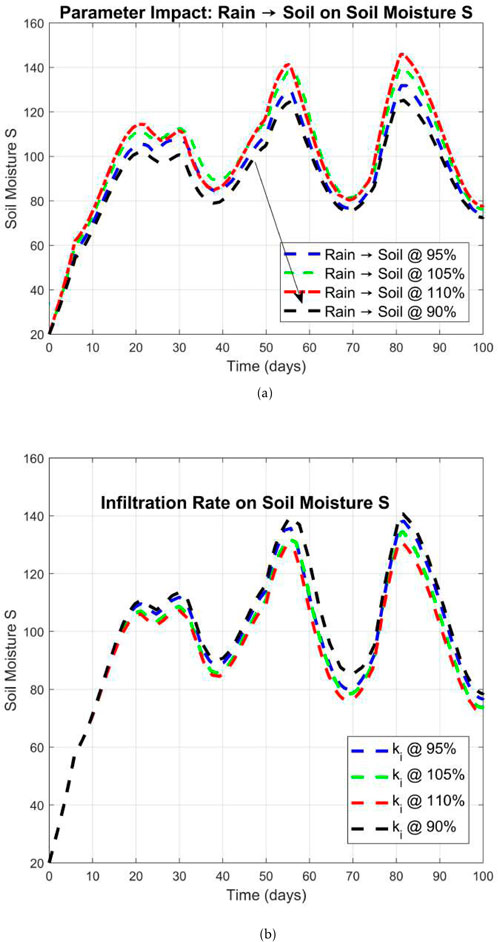
Figure 4. Soil moisturization $\mathfrak{S}$ under the effects of surface storage and infiltration rates by the FF-flood dynamical system (1.1) for the FF-orders 0.98. (a) Soil moisture variation under the effects of rain fall which is contributing to the surface storage as a fractional part f₁. (b) Moisturization of the soil under the effects of the infiltration rates k_i.

The Figure 5 shows the importance and effects of the $f_1$ over the flood height $\mathcal{H}$ and surface runoff ${\mathfrak{Q}}_s$. It is observed that for the minimum value of $f_1$ the flood height is highest shown in the Figure 5a. This is further impacting the surface runoff ${\mathfrak{Q}}_s$ given in the Figure 5b. The minimum $f_1$ level has shown the maximum surface runoff in the comparative graphs expressed by the dotted black line.

Figure 5

Figure 5. Flood raise and surface runoff caused by the rain fall with variation of the surface storage rates $f_1$ of the FF-dynamical system (1.1) of FF-orders 0.98. (a) Flood dynamics H under the effects of the Rain to soil infiltration caused by the fraction of the rain fall aiding to the surface storage f₁ of the FF-Flood system (1.1). (b) The surface runoff under the variations in the f₁ values of the model (1.1) for the FF-orders 0.98.

The heatmap describes the flood height $\mathcal{H}$ with deviations in the river overflow factor $\varphi$ and river capacity $Q_{\text{cap}}$. The data of $\varphi$ varies from 0.8 to 1.2, while ${\mathfrak{Q}}_{\text{cap}}$ also has the same variation limits ranging from 0.8 to 1.2 times its baseline value of 35. The color scale shows the flood height indicated during the computations. Higher flood level (up to 300 units) is recorded when $\varphi >1.15$ and ${\mathfrak{Q}}_{\text{cap}}<0.9\times 35$, showing conditions where river overflow is frequent and more intense. While, low $\varphi$ and high ${\mathfrak{Q}}_{\text{cap}}$ limit flooding.

In Figures 6–8, surface runoff, and cumulative frequency distribution of flood height impacted with the help of the infiltration rates and river capacity of the FF-flood dynamical system (1.1) of FF-orders 0.98 are given. In Figure 7a, the flow duration curve (FDC) compares river flow rates $Q_r$ under variation in the values for the surface storage depletion rate $f_2$. The x-axis represents ${\mathfrak{Q}}_r$ in $m^3/s$, ranging up to 250, while the y-axis shows exceedance probability from 0 to 1. Four cases are expressed: $f_2$ at 90%, 95%, 105%, and 110%. The dashed yellow line (110%) shows the highest flow for low-probability cases (e.g., $Q_r\approx 225$ at 0.1), showing more severe flood potential. While the black dashed line (90%) represents reduced flow values, particularly below 150 $m^3/s$ for high exceedance probabilities above 0.5. In Figure 7b the heatmap describes the deviation in flood height $H$ as directed by parameters $f_1$ and $\lambda$. The $f_1$ and $\lambda$ ranges from 0.8 to 1.2. Elevated flood heights above 500 are observed for lower $f_1$ and higher $\lambda$ values, indicating magnified surface water accumulation due to limited infiltration and reduced channel discharge efficiency. Conversely, as $f_1$ improves beyond 1.0, $H$ is significantly decreased to 150, which is demanding enhanced drainage conditions.

Figure 6

Figure 6. Surface runoff and flood height impacted with the help of the infiltration rates and river capacity of the FF-flood dynamical system (1.1) of FF-orders 0.98. (a) Infiltration rate on the surface runoff Q_s under the influence of the k_i. (b) nnn.

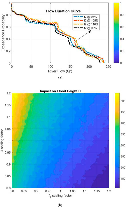
Figure 7

Figure 7. $f_1-\lambda$ scaling factors impact on the flood height observed by the dynamical system (1.1) of FF-orders 0.98. (a) f₁−λ scaling factors impact on the flood height observed by the dynamical system (1.1) of FF-orders 0.98. (b) f₁−λ scaling factors impact on the flood height observed by the dynamical system (1.1) FF-orders 0.98.

Figure 8

Figure 8. Cumulative frequency distribution of water and flood heights analysis by the scaling parameters $\rho -\gamma$ of the FF-Flood dynamical system (1.1) of FF-orders 0.98. (a) Cumulative frequency distribution of river flow under the variant f₁. (b) ρ-γ-scaling impacts over the flood height FF-water cycle model (1.1) of orders 0.98.

In Figure 8b, the heatmap indicates the sensitivity of flood height $\mathcal{H}$ to the changes in the scaling parameters of infiltration loss rate $\gamma$ and flood response coefficient $\rho$. The horizontal axis represents $\rho$ in domain from 0.8 to 1.2, while the vertical axis shows $\gamma$ has the domain from 0.8 to 1.2. The colored bar on the right maps flood height values from 215 to 250, with darker blue showing lower levels (near 215) and yellow presenting higher peaks (above 250). The map presents that increases in $\rho$ and $\gamma$ can both amplify and suppress flood height, indicating a nonlinear dynamical impact.

The impact of $f_2$ variation over the soil moisturization and flood development is studied in the Figure 9. In the first Figure 9a, the soil moisturization is analyzed for the different levels of $f_2$ but it is observed that for the least water dissipation, the moisturization level is the highest throughout the period of the study. And in contrast, the dissipation level for the largest level of the $f_2$ is maximum shown in the Figure 9b.

Figure 9

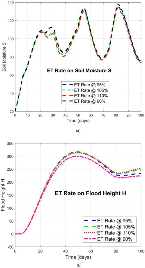
Figure 9. The impact of $f_2$ over the soil moisturization and amplifying the height of the flood studied by the FF-Flood dynamical model (1.1) for the FF-orders 0.98. (a) The impact of f₂ over the soil moisturization. (b) Flood height analysis based on the variation of the f₂.

The Figure 10 describes the cumulative frequency distribution dynamics based on the variation in river flow $Q_r$ as a function of cumulative probability under different scaling cases of the runoff generation factor $f_1$. An increase in $f_1$ from 90% to 110% shifts the curves rightward, indicating higher discharge rates becoming more probable. Notably, the 110% case accumulates higher flows more rapidly, while the 90% curve representing limited runoff contribution. This highlights the sensitivity of flow regimes to runoff efficiency, where increased $f_1$ enhances river discharge volumes and intensifying flood risks and altering hydrological stability.

Figure 10

Figure 10. Cumulative probability for the frequency distribution over river flow ${\mathfrak{Q}}_r$ of the FF-Flood dynamical system (1.1) for the variant $f_1$.

3.1.1 Table 1: impact of parameter variations scaled by 0.95

Table 2 highlights the role of reducing each hydrological parameter by 5% on five state variables: soil moisture $(\mathfrak{S})$, surface runoff $({\mathfrak{Q}}_s)$, river flow $({\mathfrak{Q}}_r)$, water height $(\mathcal{H})$, and flood-affected area $({\mathfrak{A}}_f)$. The parameters impacted include: fraction of rainfall contributing to surface storage $(f_1)$, depletion in the surface storage $(f_2)$, infiltration coefficient $(k_i)$, rainfall-to-runoff ratio $(\eta )$, soil storage threshold $(\theta )$, runoff-to-river rate $(\lambda )$, and river overflow rate $(\varphi )$. Decrease in $f_1$ significantly increases $\mathfrak{S}$ while reducing ${\mathfrak{Q}}_r$, $\mathcal{H}$, and ${\mathfrak{A}}_f$. Slightly reducing $f_2$ and $k_i$ increases $\mathfrak{S}$, as less water exits the soil via evapotranspiration and infiltration. And reducing $\eta$ greatly reduces ${\mathfrak{Q}}_s$, ${\mathfrak{Q}}_r$, $\mathcal{H}$, and ${\mathfrak{A}}_f$. The most sensitivity of $\theta$ is observed when reduced it enhances ${\mathfrak{Q}}_r$ and ${\mathfrak{A}}_f$, showing flood intensification due to diminished soil holding capacity. The reductions in $\lambda$ and $\varphi$ cause delayed river flow and overflow, gradually. Overall, even small negative perturbations to these parameters variate the flood expansion pathways.

Table 2

Table 2. Impact of parameter variations scaled by 0.95.

3.1.2 Table 2: impact of parameter variations scaled by 1.05

Table 2 evaluates the system’s response to a 5% increase in the same set of hydrological parameters. Increasing $f_1$ (rainfall into soil) reduces soil moisture $S$, likely due to quicker infiltration and dispersion through the soil profile. Interestingly, $Q_r$, $H$, and $A_f$ also decrease, implying less water is reaching the downstream flood zones. In contrast, increasing $f_2$ (evapotranspiration) leads to a decrease in $S$ and slight increases in $Q_r$ and $H$, suggesting that a more active water cycle accelerates water movement. An increase in $\eta$ (rain-to-runoff efficiency) significantly elevates $Q_r$, $H$, and $A_f$, due to faster surface water movement. Higher $\theta$ reduces $Q_s$ and downstream values, implying that a higher storage threshold buffers runoff. Notably, an increase in $\lambda$ and $\varphi$ amplifies both $Q_r$ and $A_f$, as water transfers more efficiently into the river and overflows to flood zones. These outcomes confirm the model’s sensitivity to small positive deviations and suggest control strategies focused on modifying these parameters to reduce flood impact.

3.1.3 Table 3: impact of parameter variations scaled by 1.10

Table 3 explores the influence of a 10% increase in each hydrological parameter. A sharp rise in $f_1$ drastically reduces $Q_r$, $H$, and $A_f$, indicating that diverting more rain into the soil dampens flood severity. In contrast, increasing $\eta$ and $\lambda$ greatly intensifies $Q_r$ and $A_f$, indicating that more efficient runoff and quicker river discharge dramatically elevate flood risks. The increase in $f_2$ has minimal effect on the variables, suggesting the evapotranspiration rate plays a moderate role in the overall system behavior. Notably, an increase in $\theta$ (soil storage threshold) decreases downstream impacts, confirming its buffering role. Meanwhile, the higher overflow rate $(\varphi )$ significantly increases $A_f$, emphasizing the importance of overflow infrastructure in floodplain management. These results demonstrate non-linear dynamics: some parameters like $\eta$ and $\lambda$ strongly control flood escalation, while others such as $f_2$ show more passive influence. Thus, proper calibration and structural mitigation targeting high-impact parameters could be effective in reducing vulnerability to extreme flood events. A similar illustration is given in the Tables 3, 4.

Table 3

Table 3. Impact of parameter variations scaled by 1.05.

Table 4

Table 4. Impact of parameter variations scaled by 1.10.

4 Deep learning analysis of flood dynamical system

Training an AI model for getting an optimal function $f$ that integrate input data $X$ to output $Y$ and to minimizes a loss function $L(f(X),Y)$ by the help of parameters adjustments are illustrated for the FF-Flood dynamical system (1.1) in this section. The optimization algorithm is illustrated by:

${\zeta }^{\left(t+1\right)}={\zeta }^{\left(t\right)}-{\eta }_0\nabla L\left({\theta }^{\left(t\right)}\right),(4.1)$

where, in Equation 4.1, the $\zeta$ represents model parameters (weights, biases) ${\eta }_0$ is the learning rate, $\nabla L(\zeta )$ is the gradient of the loss function. The use of ${\eta }_0$ largely impacts convergence. Too large a value leads to instability, while too small a value slow the convergence. In Figure 11a, the simulation data is trained for the deep learning of the FF-Flood dynamical system (1.1) for the FF-orders 0.98.

The MSE is calculated by the following formula: $MSE=\frac{1}{n}{\sum }_{i=1}^n{({\mathcal{F}}_i-{\widehat{\mathcal{F}}}_i)}^2$, where ${\widehat{\mathcal{F}}}_i$, is the predicted output. The validation performance was determined to measure the model’s potential to generalize the unseen data during training. Cross-validation technique was utilized to partition the dataset into training and validation subsets. Notably, the optimal validation outcome was obtained at the 987th epoch, yielding a minimum error of $2.6298\times 10^{-06}$.

4.1 Mean square error

This section is dedicated to the AI based analysis for mean square error of the computational data driven from the FF-flood dynamical system (1.1). For this, 998 data points were considered. In this data, 499 points were assumed as the input data points while 499 points as the target data points. The data was trained under Levenberg-Marquardt principles given in the Figure 11. A gradient 0.00033837 was recorded for the epoch 987 with $\mu =1\times 10^{-05}$ in the and best validation performance was noted as $2.6298\times 10^{-06}$ at 987th epoch in the Figures 11a,b, respectively. The data analysis has shown a decreasing mean square error graph.

$\text{MSE}=\frac{1}{m}{\displaystyle \sum _{i=1}^m}{\left({\mathcal{F}}_i-{\widehat{\mathcal{F}}}_i\right)}^2,$

where ${\mathcal{F}}_i$ are actual values, ${\widehat{\mathcal{F}}}_i$ are predicted values, and $m$ is the number of data points. A lower MSE shows better model accuracy. The BVF marks the optimal point where the model generalizes well to unseen data without overfitting or underfitting.

Figure 11

Figure 11. Training the models data for the deep learning based analysis FF-flood dynamical system (1.1) with best validation performance $2.6298\times 10^{-06}$ at 987th epoch. (a) Training of the data for the deep learning of complex FF-Flood dynamical model (1.1) for the FF-orders 0.98. (b) Mean Square Error for the complex FF-Flood dynamical model (1.1), for the FF-orders 0.98.

The Figure 12 is presenting error recognition and regression analysis of the data for the FF-Flood dynamical system (1.1). In the Figure 12a, the error histogram is showing the error around zero error for the validation, training, and testing data. The Figure 12b is describing the regression of the data which is shown as $R=1$, which is confirming the best approach of the data analysis with the help of the artificial intelligence.

Figure 12

Figure 12. Deep learning results for water cycle mechanism (1.1) for the FF-orders 0.98 by Levenberg-Marquardt techniques for regression and error estimations. (a) Error histogram with 20 bins representing the zero error, training data set, validation, and testing data for the FF-Flood dynamical system (1.1). (b) Regression in the training, validation and test data sets for FF-Flood dynamical system (1.1).

4.2 Regression of the data

The regression models are used to predict continuous values in corresponding to the input data points. We use linear and logistic regression for this analysis. The mathematical expression behind the linear regression is:

$Y={\vartheta }_0^{⊛}+{\vartheta }_1^{⊛}{\mathcal{U}}_1+{\vartheta }_2^{⊛}{\mathcal{U}}_2+\cdots +{\vartheta }_n^{⊛}{\mathcal{U}}_n+{ϵ}^{⊛},(4.2)$

in Equation 4.2, $ϵ⊛$ is denoting the random error. The ${\vartheta }^{⊛}$ is produced the following optimization procedure Equation 4.3 is expressed:

$\widehat{{\vartheta }^{⊛}}={\left({\mathcal{U}}^T\mathcal{U}\right)}^{-1}{\mathcal{U}}^{T}Y(4.3)$

While the logistic regression generates the probability of a data and is based on the following relationship Equation 4.4:

$P\left(Y=1|\mathcal{U}\right)=\frac{1}{1+e^{-\left({\vartheta }_0^{⊛}+{\vartheta }_1^{⊛}{\mathcal{U}}_1+\cdots +{\vartheta }_n^{⊛}{\mathcal{U}}_n\right)}}(4.4)$

This function, ensures output probabilities in between 0, and 1. An error histogram for the error distribution is computed as in Equation 4.5:

$E_i={{}_m\mathcal{G}}_i-m{\widehat{\mathcal{G}}}_i,(4.5)$

where, ${{}_m\mathcal{G}}_i$ are the actual values of the membrane potential while $m{\widehat{\mathcal{G}}}_i$ are the predicted values. One can see some more relevant works on the topic in Wan-Arfah et al. (2023). The regression data is presented in the four subgraphs. The first subgraph is about the training data where the $Output\approx 1\times Target+7.4^{-07}$ which has given the regression $R=1$. For the validation portion, the output is obtained with the perturbation relation: $Output\approx 1\times Target-7.3^{-05}$. The test data set has used the output relationship $Output\approx 1\times Target+8.5^{-05}$. The accumulative regression is measured by the relationship $Output\approx 1\times Target+2.3^{-06}$. This error was evaluated by the relationship $Error=Targets-Outputs$.

In Figure 13, the neural networking is applied for the dynamical studies of the actual with the prediction data sets. It is observed that there is a very close similarity in the simulations for all the classes between the actual and the predicted data sets. The state 1 is showing the NN vs. actual comparison for the surface storage $\mathfrak{S}$. The actual data is represented by the red dotted line while the NN prediction is presented by the green dashed line. State 2 is about the surface runoff ${\mathfrak{Q}}_s$, the ${\mathfrak{Q}}_r$ is compared for the real and predicted data sets, The water level $\mathcal{H}$. The final graph is for the affected area by the flood studied under the FF-Flood dynamical system (1.1). All these simulations are obtained for the FF-orders 0.98. Figure 13 compares neural network predictions with actual data for hydrological variables, showing close agreement. It includes surface storage $\mathfrak{S}$, runoff ${\mathfrak{Q}}_s$, discharge ${\mathfrak{Q}}_r$, water level $\mathcal{H}$, and flood-affected areas using the FF-Flood model.

Figure 13

Figure 13. Neural-network predictions vs. actual data sets of the variables of the FF-Flood dynamical system (1.1) for the FF-orders 0.98.

5 Conclusion

In this paper we considered a FF-flood dynamical system for the solution existence with stability results for the Hyers-Ulam type, numerical simulations and AI-based deep learning. The paper is structured for the computational results therefore the qualitative analysis is not given with their proofs. Although, we highlighted the related works from the available literature. In Section 2, the theoretical results are given related to the presumed model (1.1). In the Section 3, we have developed a numerical scheme based on the Lagrange’s interpolation polynomial for the simulations of the model. The scheme is then applied to an illustrative example for soil moisturization, water level raise and depletion affecting the flood dynamics. For lower $f_1$ and higher $f_2$, the maximum surface runoff is observed. Also, the flood is getting higher level for the lower level of the rain infiltration.

The Figure 12 is presenting error recognition and regression analysis of the data for the FF-Flood dynamical system (1.1). In the Figure 12a, the error histogram is showing the error around zero error for the validation, training, and testing data. The subfigure 12b is describing the regression of the data which is shown as $R=1$, which is confirming the best approach of the data analysis with the help of the artificial intelligence. The regression data is presented in the four subgraphs. The first subgraph is about the training data where the $Output\approx 1\times Target+7.4\times 10^{-07}$ which has given the regression $R=1$. For the validation portion, the output is obtained with the perturbation relation: $Output\approx 1\times Target-7.3\times 10^{-05}$.

The study can be continued in a number of ways with consideration of more variables, parameters and different transmission rates for different regions. We highlight the following few points:

$•$ Model Integration with Ecosystem Factors: Including ecosystem variables such as vegetation and soil properties to incorporate their impacts on flood dynamics.

$•$ Data-Driven Calibration: Improving model significance by the help of remote sensing and hydrological data for real-time estimations.

$•$ Climate Change Impact Analysis: Extending the model to simulate flood behavior under future climate scenarios with the increase in atmospheric gases and temperature.

$•$ Multi-Scale Model Validation: Validating the model across different geographic factors to assess robustness.

Data availability statement

The original contributions presented in the study are included in the article/supplementary material, further inquiries can be directed to the corresponding authors.

Author contributions

HK: Methodology, Writing – review and editing, Conceptualization, Writing – original draft. RA: Conceptualization, Validation, Writing – review and editing, Visualization. JA: Writing – review and editing, Conceptualization, Supervision, Validation, Visualization. RT: Validation, Writing – review and editing, Investigation, Software.

Funding

The author(s) declare that no financial support was received for the research and/or publication of this article.

Acknowledgments

The Researchers would like to thank the Deanship of Graduate Studies and Scientific Research at Qassim University for financial support (QU-APC-2025).

Conflict of interest

The authors declare that the research was conducted in the absence of any commercial or financial relationships that could be construed as a potential conflict of interest.

Generative AI statement

The author(s) declare that no Generative AI was used in the creation of this manuscript.

Any alternative text (alt text) provided alongside figures in this article has been generated by Frontiers with the support of artificial intelligence and reasonable efforts have been made to ensure accuracy, including review by the authors wherever possible. If you identify any issues, please contact us.

Publisher’s note

All claims expressed in this article are solely those of the authors and do not necessarily represent those of their affiliated organizations, or those of the publisher, the editors and the reviewers. Any product that may be evaluated in this article, or claim that may be made by its manufacturer, is not guaranteed or endorsed by the publisher.

References

Ahmad, I., Bakar, A. A., Ahmad, H., Khan, A., and Abdeljawad, T. (2024). Investigating virus spread analysis in computer networks with Atangana–Baleanu fractional derivative models. Fractals 2440043, 17. doi:10.1142/S0218348X24400437

CrossRef Full Text | Google Scholar

Amnuaylojaroen, T. (2023). Perspective on the era of global boiling: a future beyond global warming. Adv. Meteorology 2023 (1), 1–12. doi:10.1155/2023/5580606

CrossRef Full Text | Google Scholar

An, R., Ji, M., and Zhang, S. (2018). Global warming and obesity: a systematic review. Obes. Rev. 19 (2), 150–163. doi:10.1111/obr.12624

PubMed Abstract | CrossRef Full Text | Google Scholar

Atangana, A. (2017). Fractal-fractional differentiation and integration: connecting fractal calculus and fractional calculus to predict complex system. Fractals 102, 396–406. doi:10.1016/j.chaos.2017.04.027

CrossRef Full Text | Google Scholar

Atangana, A., and Araz, S. I. (2020). Atangana–Seda numerical scheme for Labyrinth attractor with new differential and integral operators. Fractals 28 (08), 2040044. doi:10.1142/s0218348x20400447

CrossRef Full Text | Google Scholar

Atangana, A., and Qureshi, S. (2019). Modeling attractors of chaotic dynamical systems with fractal–fractional operators. Chaos, Solit. and fractals 123, 320–337. doi:10.1016/j.chaos.2019.04.020

CrossRef Full Text | Google Scholar

Badawy, A., Sultan, M., Abdelmohsen, K., Yan, E., Elhaddad, H., Milewski, A., et al. (2024). Floods of Egypt’s Nile in the 21st century. Sci. Rep. 14 (1), 27031. doi:10.1038/s41598-024-77002-8

PubMed Abstract | CrossRef Full Text | Google Scholar

Barry, S. M., Davies, G. R., Forton, J., Williams, S., Thomas, R., Paxton, P., et al. (2025). Trends in low global warming potential inhaler prescribing: a UK-wide cohort comparison from 2018-2024. npj Prim. Care Respir. Med. 35 (1), 9. doi:10.1038/s41533-025-00415-z

PubMed Abstract | CrossRef Full Text | Google Scholar

Bas, E., Acay, B., and Ozarslan, R. (2019). Fractional models with singular and non-singular kernels for energy efficient buildings. Chaos Interdiscip. J. Nonlinear Sci. 29 (2), 023110. doi:10.1063/1.5082390

PubMed Abstract | CrossRef Full Text | Google Scholar

Böttcher, L., Antulov-Fantulin, N., and Asikis, T. (2022). AI Pontryagin or how artificial neural networks learn to control dynamical systems. Nat. Commun. 13 (1), 333. doi:10.1038/s41467-021-27590-0

PubMed Abstract | CrossRef Full Text | Google Scholar

Cai, W., Zhang, C., Zhang, S., Bai, Y., Callaghan, M., Chang, N., et al. (2024). The 2024 China report of the Lancet Countdown on health and climate change: launching a new low-carbon, healthy journey. Lancet Public Health 9 (12), e1070–e1088. doi:10.1016/s2468-2667(24)00241-x

PubMed Abstract | CrossRef Full Text | Google Scholar

Cao, M., Wang, F., Ma, S., Geng, H., and Sun, K. (2024). Recent advances on greenhouse gas emissions from wetlands: mechanism, global warming potential, and environmental drivers. Environ. Pollut. 355, 124204. doi:10.1016/j.envpol.2024.124204

PubMed Abstract | CrossRef Full Text | Google Scholar

Caputo, M., and Fabrizio, M. (2015). A new definition of fractional derivative without singular kernel. Prog. Fract. Differ. Appl. 1 (2), 73–85. doi:10.12785/pfda/010201

CrossRef Full Text | Google Scholar

Clarke, R. H., Wescombe, N. J., Huq, S., Khan, M., Kramer, B., and Lombardi, D. (2023). Climate loss-and-damage funding: a mechanism to make it work. Nature 623 (7988), 689–692. doi:10.1038/d41586-023-03578-2

PubMed Abstract | CrossRef Full Text | Google Scholar

Darvishi Boloorani, A., Nasiri, N., Soleimani, M., Papi, R., Neysani Samany, N., Amiri, F., et al. (2024). “Climate change, dust storms, and air pollution in the MENA Region,” in Climate change and environmental degradation in the MENA Region 2024. Cham: Springer Nature Switzerland, 327–343.

CrossRef Full Text | Google Scholar

Gabr, M. E. (2023). Impact of climatic changes on future irrigation water requirement in the Middle East and North Africa’s region: a case study of upper Egypt. Appl. Water Sci. 13 (7), 158. doi:10.1007/s13201-023-01961-y

CrossRef Full Text | Google Scholar

Gazi, M. A., Al Masud, A., Rahman, M. K., Amin, M. B., Emon, M., bin, S., et al. (2025). Sustainable embankment contribute to a sustainable economy: the impact of climate change on the economic disaster in coastal area. Environ. Dev. 55, 101208. doi:10.1016/j.envdev.2025.101208

CrossRef Full Text | Google Scholar

Gebrael, K., Mitri, G., and Kalantzi, O. I. (2024). Overview of nature-based solutions for climate resilience in the MENA region. Nature-Based Solutions 6, 100159. doi:10.1016/j.nbsj.2024.100159

CrossRef Full Text | Google Scholar

Hamed, M. M., Sobh, M. T., Ali, Z., Nashwan, M. S., and Shahid, S. (2024). Aridity shifts in the MENA region under the Paris agreement climate change scenarios. Glob. Planet. Change 238, 104483. doi:10.1016/j.gloplacha.2024.104483

CrossRef Full Text | Google Scholar

Herrmann, R. (2011). Fractional calculus: an introduction for physicists. World Sci. doi:10.1142/9789814340250

CrossRef Full Text | Google Scholar

Janni, M., Maestri, E., Gullì, M., Marmiroli, M., and Marmiroli, N. (2024). Plant responses to climate change, how global warming may impact on food security: a critical review. Front. Plant Sci. 14, 1297569. doi:10.3389/fpls.2023.1297569

PubMed Abstract | CrossRef Full Text | Google Scholar

Jonkman, S. N., Curran, A., and Bouwer, L. M. (2024). Floods have become less deadly: an analysis of global flood fatalities 1975–2022. Nat. Hazards 120 (7), 6327–6342. doi:10.1007/s11069-024-06444-0

CrossRef Full Text | Google Scholar

Khan, H., Aslam, M., Rajpar, A. H., Chu, Y. M., Etemad, S., Rezapour, S., et al. (2024). A new fractal-fractional hybrid model for studying climate change on coastal ecosystems from the mathematical point of view. Fractals 32 (02), 2440015. doi:10.1142/s0218348x24400152

CrossRef Full Text | Google Scholar

Khan, A., Shah, K., Abdeljawad, T., and Alqudah, M. A. (2022). Existence of results and computational analysis of a fractional order two strain epidemic model. Results Phys. 39, 105649. doi:10.1016/j.rinp.2022.105649

CrossRef Full Text | Google Scholar

Khan, A., Abdeljawad, T., Abdel-Aty, M., and Almutairi, D. K. (2025a). Digital analysis of discrete fractional order cancer model by artificial intelligence. Alexandria Eng. J. 118, 115–124. doi:10.1016/j.aej.2025.01.036

CrossRef Full Text | Google Scholar

Khan, A., Abdeljawad, T., and Alkhawar, H. M. (2025b). Digital analysis of discrete fractional order worms transmission in wireless sensor systems: performance validation by artificial intelligence. Model. Earth Syst. Environ. 11 (1), 25. doi:10.1007/s40808-024-02237-3

CrossRef Full Text | Google Scholar

Khan, H., Alzabut, J., Almutairi, D. K., and Alqurashi, W. K. (2025c). The use of artificial intelligence in data analysis with error recognitions in liver transplantation in HIV-AIDS patients using modified ABC fractional order operators. Fractal Fract. 9 (1), 16. doi:10.3390/fractalfract9010016

CrossRef Full Text | Google Scholar

Khan, H., Alzabut, J., Tounsi, M., and Almutairi, D. K. (2025d). AI-Based data analysis of contaminant transportation with regression of oxygen and nutrients measurement. Fractal Fract. 9 (2), 125. doi:10.3390/fractalfract9020125

CrossRef Full Text | Google Scholar

Kumar, V. R., and Mani, N. (1994). The application of artificial intelligence techniques for intelligent control of dynamical physical systems. Int. J. Adapt. Control Signal Process. 8 (4), 379–392. doi:10.1002/acs.4480080407

CrossRef Full Text | Google Scholar

Kumar, P., Erturk, V. S., Banerjee, R., Yavuz, M., and Govindaraj, V. (2021). Fractional modeling of plankton-oxygen dynamics under climate change by the application of a recent numerical algorithm. Phys. Scr. 96 (12), 124044. doi:10.1088/1402-4896/ac2da7

CrossRef Full Text | Google Scholar

Kurniawan, T. A., Meidiana, C., Goh, H. H., Zhang, D., Jiang, M., Othman, M. H. D., et al. (2024). Social dimensions of climate-induced flooding in Jakarta (Indonesia): the role of non-point source pollution. Water Environ. Res. 96 (9), e11129. doi:10.1002/wer.11129

PubMed Abstract | CrossRef Full Text | Google Scholar

Nan, Y., Bao-hui, M., and Chun-Kun, L. (2011). Impact analysis of climate change on water resources. Procedia Eng. 24, 643–648. doi:10.1016/j.proeng.2011.11.2710

CrossRef Full Text | Google Scholar

Ripple, W. J., Wolf, C., Gregg, J. W., Rockström, J., Mann, M. E., Oreskes, N., et al. (2024). The 2024 state of the climate report: perilous times on planet Earth. BioScience 74 (12), 812–824. doi:10.1093/biosci/biae087

CrossRef Full Text | Google Scholar

Rogers, J. S., Maneta, M. M., Sain, S. R., Madaus, L. E., and Hacker, J. P. (2025). The role of climate and population change in global flood exposure and vulnerability. Nat. Commun. 16 (1), 1287. doi:10.1038/s41467-025-56654-8

PubMed Abstract | CrossRef Full Text | Google Scholar

Sabatier, J. A., Agrawal, O. P., and Machado, J. T. (2007). Advances in fractional calculus. Dordrecht: Springer.

Google Scholar

Salhi, A., Benabdelouahab, S., and Heggy, E. (2024). Observation and geoinformation. Int. J. Appl. Earth Observation Geoinformation 133 (10413), 2. doi:10.1016/j.jag.2024.104132

CrossRef Full Text | Google Scholar

Sekerci, Y. (2020). Climate change effects on fractional order prey-predator model. Chaos, Solit. Fractals 134, 109690. doi:10.1016/j.chaos.2020.109690

CrossRef Full Text | Google Scholar

Sharma, P., Khan, J. S., Radhika, K., Thatipudi, J. G., Sridevi, K., and Upadhyay, S. (2025). “Evolutionary intelligence: a hybrid neural framework for dynamic system innovation,” in 2025 international conference on electronics and renewable systems (ICEARS) (IEEE), 1743–1749.

Google Scholar

Su, Y., and Ullah, K. (2024). Exploring the correlation between rising temperature and household electricity consumption: an empirical analysis in China. Heliyon 10 (10), e30130. doi:10.1016/j.heliyon.2024.e30130

PubMed Abstract | CrossRef Full Text | Google Scholar

Sun, H., Zhang, X., Ruan, X., Jiang, H., and Shou, W. (2024). Mapping compound flooding risks for urban resilience in coastal zones: a comprehensive methodological review. Remote Sens. 16 (2), 350. doi:10.3390/rs16020350

CrossRef Full Text | Google Scholar

Terry, J. P., Al Ruheili, A., Almarzooqi, M. A., Almheiri, R. Y., and Alshehhi, A. K. (2023). The rain deluge and flash floods of summer 2022 in the United Arab Emirates: causes, analysis and perspectives on flood-risk reduction. J. Arid Environ. 215, 105013. doi:10.1016/j.jaridenv.2023.105013

CrossRef Full Text | Google Scholar

Trenberth, K. E. (2014). Water cycles and climate change. Glob. Environ. Change 2014, 31–37. doi:10.1007/978-94-007-5784-4_30

CrossRef Full Text | Google Scholar

Van Daalen, K. R., Tonne, C., Semenza, J. C., Rocklöv, J., Markandya, A., Dasandi, N., et al. (2024). The 2024 Europe report of the lancet countdown on health and climate change: unprecedented warming demands unprecedented action. Lancet Public Health 9 (7), e495–e522. doi:10.1016/s2468-2667(24)00055-0

PubMed Abstract | CrossRef Full Text | Google Scholar

Van Houtven, G. (2024). Economic value of flood forecasts and early warning systems: a review. Nat. Hazards Rev. 25 (4), 03124002. doi:10.1061/nhrefo.nheng-2094

CrossRef Full Text | Google Scholar

Wan-Arfah, N., Muzaimi, M., Naing, N. N., Subramaniyan, V., Wong, L. S., and Selvaraj, S. (2023). Prognostic factors of first-ever stroke patients in suburban Malaysia by comparing regression models. Electron. J. General Med. 20 (6), em545. doi:10.29333/ejgm/13717

CrossRef Full Text | Google Scholar

Wang, Z., Leung, M., Mukhopadhyay, S., Sunkara, S. V., Steinschneider, S., Herman, J., et al. (2024). A hybrid statistical–dynamical framework for compound coastal flooding analysis. Environ. Res. Lett. 20 (1), 014005. doi:10.1088/1748-9326/ad96ce

CrossRef Full Text | Google Scholar

Wu, Y., Liu, S., and Gallant, A. L. (2012). Predicting impacts of increased CO2 and climate change on the water cycle and water quality in the semiarid James River Basin of the Midwestern USA. Sci. Total Environ. 430, 150–160. doi:10.1016/j.scitotenv.2012.04.058

PubMed Abstract | CrossRef Full Text | Google Scholar

Yang, K., Wu, H., Qin, J., Lin, C., Tang, W., and Chen, Y. (2014). Recent climate changes over the Tibetan Plateau and their impacts on energy and water cycle: a review. Glob. Planet. Change 112, 79–91. doi:10.1016/j.gloplacha.2013.12.001

CrossRef Full Text | Google Scholar

Yaseen, R. M., Ali, N. F., Mohsen, A. A., Khan, A., and Abdeljawad, T. (2024). The modeling and mathematical analysis of the fractional-order of Cholera disease: dynamical and simulation. Partial Differ. Equations Appl. Math. 12, 100978. doi:10.1016/j.padiff.2024.100978

CrossRef Full Text | Google Scholar

Yuksel, G. (2024). Dynamical systems and artificial intelligence. Artificial Intell. 29, 75–83. doi:10.1201/9781003483571-6

CrossRef Full Text | Google Scholar