 Łukasz Sobol
 Jacek A. Koziel
 Sylwia Stegenta-Dąbrowska
- 1Energy, Environment and Society Centre, Wrocław University of Environmental and Life Sciences, Wrocław, Poland
- 2Department of Applied Bioeconomy, Wroclaw University of Environmental and Life Sciences, Wroclaw, Poland
- 3USDA-ARS Conservation and Production Research Laboratory, Bushland, TX, United States
- 4Department of Agricultural and Biosystems Engineering, Iowa State University, Ames, IA, United States
Sports turfs and urban landscapes generate waste biomass in the form of grass clippings. Decomposing grass clippings can recycle nutrients to soil. However, decomposing can have adverse environmental effects such as gaseous emissions. The magnitude of air pollution caused by gaseous emissions from grass clippings is unknown. This research investigated CO, CO2, and O2 exchange during the decomposition of grass clippings. Emissions from grass clippings collected at four football fields with different levels of fertilization and agrotechnical treatments were studied. The mowed grass was collected throughout the spring-to-autumn football season. The results showed that grass clippings from sports turfs can generate up to 5 times more CO emissions compared to a mixture of grass and cattle manure. CO2 production and O2 consumption were relatively similar for all seasons, except for clippings from the unfertilized pitch. Artificial neural network (ANN) models predicted the CO and CO2 emissions resulting from the disposal of grass clippings with R2 for CO > 0.81 and CO2 > 0.98, respectively. This research contributes to emission inventories and highlights the relatively minor contribution from decomposing biomass.
1 Introduction
Grass mowing is an indispensable agrotechnical treatment performed on sport turfs to maintain their quality, including increased turf density, improved playability and resistance to wear (Linde, 2015; March et al., 2013). Depending on the purpose and type of sports grass surface, it can be mowed nearly 200 times a year (Tidåker et al., 2017). Due to the high frequency of treatments, significant amounts of grass clippings are generated during mowing, requiring proper disposal. Previous research have shown that it is possible to generate as much as 7.2 Mg DM∙y-1∙ha-1 grass clippings from sports grass surfaces during the season (Grossi et al., 2004). The dry matter (DM) yield from grass sports surfaces is relatively high compared to similar managed landscapes (Table 1).
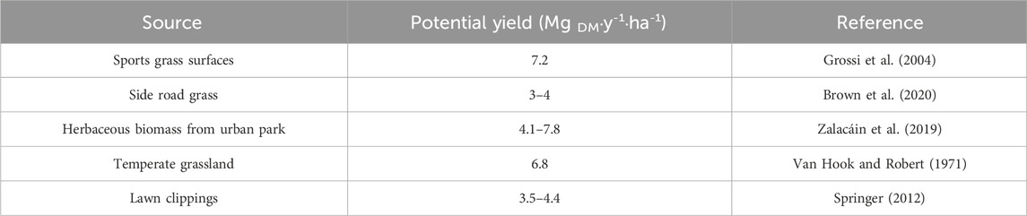
Table 1. Comparison of biomass yield from sport surfaces to other grass surfaces.
Despite the suitability of grass clippings for mulching, composting, and biogas production, some sports facilities classify clippings as ‘waste’ and therefore, leaving them as-is in random locations to decompose and reduce weight and volume. Thus, there is a concern about the impact of such poorly managed biomass on the environment. Microbiological activity can increase greenhouse gas (GHG) (CO2, N2O, and CH4) emissions and leaching our of toxic substances to soil (Boldrin et al., 2009; Haarstad et al., 2006; Stegenta-Dąbrowska et al., 2020; Figure 1).
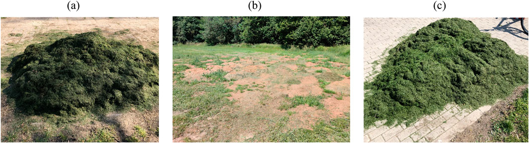
Figure 1. Uncontrolled disposal of grass clippings from mowing sports turfs; (a) on soil; (b) effect of grass clippings from a small football field (0.7 ha) on vegetation, (c) on paver stones.
To date, research has focused on gaseous emissions related to managed grass surfaces, in particular, GHGs (Bremer, 2006; Follett et al., 2011; Law et al., 2021; Van Delden et al., 2016), carbon sequestration in the soil (Qian and Follett, 2002; Zirkle et al., 2011) or the use of specialized equipment to perform agrotechnical and pratotechnical treatments (Montgomery, 2009). There is a gap in knowledge about gaseous emissions from the decomposition or poorly managed composting of grass clippings. Specifically, the emission rates of primary air pollutants such as CO are not well known. Due to its odorless, tasteless, colorless nature, and toxicity, CO poses a significant risk to human health and living organisms, including most microorganisms (Stegenta-Dąbrowska et al., 2020; Techtmann et al., 2009; Afzal et al., 2025).
Gaseous emissions from composting green waste can be managed (Sobieraj et al., 2021). The spatial and temporal variability of CO emissions from managed, industrial scale composting operations was reported (Stegenta et al., 2019a; Stegenta et al., 2019b). However, the uncontrolled decomposition of grass clippings makes it challenging to estimate the CO and CO2 production rate and emission to the atmosphere, as the process is affected by many environmental factors. Therefore, the determination of the kinetic parameters and predicting CO and CO2 emissions from grass clippings can improve emission source inventories. In addition, estimates of gaseous emissions from clipping associated with similarly managed residential and municipal lawns are needed as both sources are an essential element of landscape architecture (Ignatieva et al., 2020; 2024). Estimating CO emission rates allows determining the risk associated with human short-term and chronic inhalation exposure to toxic gases. This problem can be exacerbated if the clippings are spread near sports stands or in urban stadiums, negatively affecting local air quality, creating public health implications. On the other hand, there is a growing interest in generating bio-renewable CO as a key ingredient to bio-based economy which can find industrial applications (Dang and Chou, 2018; Foresti et al., 2008; Sobieraj et al., 2025). Artificial intelligence (AI) enables the evaluation and optimization of process parameters, particularly in agricultural and environmental fields (Zhong et al., 2021). For example, AI can improve the control of fermentation, composting, and waste management processes (Ye et al., 2020; Rosik et al., 2024; Cheng et al., 2023).
Our working hypothesis is that gaseous emissions (CO, CO2, and process-associated O2 utilization) from clippings are affected by management practices. Chemical composition of grass clippings depend mainly on the grass variety (Wolski et al., 2021) and the agrotechnical treatments, e.g., the fertilization and irrigation (Noer, 1945). Research show the role of moisture content (MC) on the production of CO (Schade et al., 1999). However, to the best of our knowledge there are no direct reports linking CO emissions with fertilization in the literature. Fertilization is one of the most important elements influencing the visual and functional features of the turf (Wolski et al., 2016) and the chemical composition of grass clippings (Waddington et al., 1964). Therefore, it can be also hypothesized that fertilization may affect CO emissions during the decomposition of grass clippings. Highly fertilized turfs may exceed 600 kg N∙ha-1 (Salman and Avcioglu, 2010), while the turfs of lower-league clubs are not necessarily fertilized. This research is the first attempt to quantify the magnitude of CO emissions from grass piles generated on sports turfs. These results can significantly contribute to the estimation of the inventory of emissions from sports surfaces, not limited only to football fields, but also to similar types of managed surfaces - golf courses, rugby fields, urban lawns.
This study aimed to address the following gaps in knowledge:
i. CO and CO2 emissions during the decomposition of grass clippings from sports turf under controlled laboratory conditions,
ii. the kinetics of CO emissions during the decomposition of organic matter in grass clippings,
iii. predicting the CO, CO2 emissions, and O2 consumption during the decomposition of grass clippings,
iv. identifying the main mechanisms and parameters responsible for CO emissions during the decomposition of grass clippings from sports turf, in particular the role of fertilization and season.
2 Materials and methods
2.1 Sport turfs
Grass clippings were collected immediately after mowing the turf at four football fields in the Dolnośląskie Voivodeship, Poland. The summary is presented in Table 2:
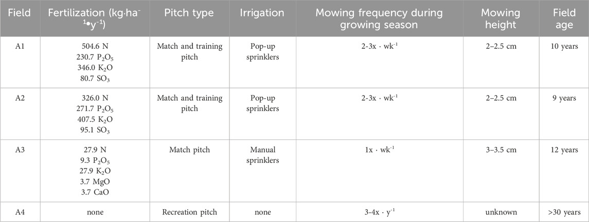
Table 2. Summary of football field characteristics.
2.2 Grass clippings properties
Samples were evaluated for their physicochemical properties before and after the decomposition process. MC was determined with the dryer (WAMED, model KBC-65W, Warsaw, Poland) according to PN-ISO 11465:1999 standard. Volatile solids (VS) were determined using a muffle furnace (SNOL, model 8.1/1100, Utena, Lithuania) according to PN-EN 15169:2011 standard. Electroconductivity and pH were evaluated on a 1:10 w/v solid/water suspension (Al-Wabel et al., 2013; Świechowski et al., 2022) using Elmetron CPC-411. CHNS Elemental Analyzer (CE Instruments Ltd., United Kingdom) was used according to PN-ISO 13878:2002 standard for C, H, and N. The respirometry activity (a.k.a. AT4) was determined according to Binner et al. (2012) with the OxiTop Control system:
where: AT4 – respirometry activity (mg O2∙g-1d.m.),
∆p–pressure difference (hPa),
MO2 – molecular mass O2 (31.998 mg∙mol-1),
R–ideal gas constant (83.14 mL∙hPa∙(K∙mol)-1),
T–temperature (293.15 K),
Vgas–total volume (mL),
Vabs–sorbent volume (mL),
Vsample–sample volume (mL),
msample–dry sample mass (g d.m.).
The kinetic parameters of the AT4 process (P0, k, t) were determined using the same method as for the process gases.
2.3 The experimental design and simulation of decomposition process
The experiment was carried out in bioreactors at a constant temperature of 20 °C (in dark), in triplicate, for grass clippings from the spring, summer, and the autumn seasons, respectively (Figure 2). Each 1 L bioreactor was filled with 15 ± 1 g of clippings. The choice of sample mass was due to preliminary trials, where different grass quantities were tested for detectable concentrations.
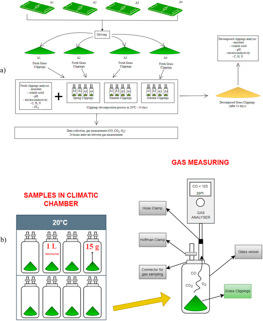
Figure 2. Scheme of the experimental set-up (a), measuring process gas production or consumption (b).
2.4 Analysis of the gas emissions
Concentrations of CO, CO2, O2 were monitored daily for 14 days. The time of 14 days was selected based on the practices of sports surface operators in the region of Lower Silesia, Poland, who decide to remove the grass clipping from the decomposition site after about 2 weeks, when they have reduced their volume. Bioreactors were equipped with sealed caps and two gas measuring ports with short sections of flexible tubing facilitating the connection to a gas analyzer for gas sampling (Figure 2b). Gaseous concentrations were measured using a factory-calibrated KIGAZ 200 gas analyzer (Kimo Instr., Chevry-Cossigny, France). Gas concentrations were measured trice for 30–50 s to stabilize the indicated values. During each measurement, the bioreactors were open to crossflow to ensure oxygen conditions in their headspace. After a few minutes of aeration, the bioreactors were closed and sealed with a Hoffman clamp and returned to the incubation chamber.
2.5 Kinetics of gas emissions
Nonlinear least squares regression was used to determine the kinetic parameters of CO and CO2 production and O2 consumption. Cumulative production and consumption curves were determined based on the d.m. of grass clippings. Zero and first-order reaction models were used:
where:
P—total production/consumption (CO, CO2, or O2), (mg·g −1 d.m.),
k—production/consumption rate (CO, CO2, or O2), (mg·g −1 d.m.·h −1),
t—time, (h).
where:
P0 — maximum production/consumption (CO, CO2, or O2), (mg·g −1 d.m.).
The average production or consumption rate (r, mg·g −1 d.m.·h −1) was estimated as:
2.6 Statistical analysis and AI modeling
Statistical analyses were performed with Statistica 13.0 (TIBCO Software Inc., Palo Alto, CA, USA). Firstly, the data distribution was checked for normality using the Shapiro-Wilk test. All variants were characterized by significantly different distributions from the normal distribution, the non-parametric Kruskal-Wallis test was performed at the α = 0.05 significance level to compare differences between variants. The results were also modeled for CO and CO2 production using ANN. First, principal component analysis (PCA) was performed to exclude parameters irrelevant to CO production. PCA analysis showed that only time, pH, CO2 production and O2 consumption are statistically significant (Supplementary Figure S1). The pH was subsequently rejected, since the pH results were measured only at the beginning and at the end of the process, and the dataset was too small to represent the group. Readers should be aware of this limitation, however, due to the fact that pH is a critical parameter in microbial decomposition. Finally, t, CO2 production and O2 consumption were used for the ANN analysis for prediction of CO and CO production and O2 consumption.
The ANN calculations were performed with Statistica 13.3 NEURAL NETWORKS environment. The 540 sets of data were randomly divided into training (75%), validation (15%), and test (15%) subsets. The differ ANN types were considered for the creation of the numerical multi-layer perception (MLP) and radial basis function network (RBF) model, and were trained with back propagation (error) training algorithms. The research covered ANN structures with one single output neuron (representing CO or CO2 production) and constant (3) inputs representing t, CO or CO2 production and O2 consumption) potentially influencing the CO or CO2 production. The network structure was evaluated by validating the set quality, and simultaneously observing training and testing set qualities (detailed ANN statistic was presented on Figure 7e). The quality parameter was calculated as the standard deviation representing the neural model prediction error divided by the standard deviation for the available original dataset in respect to the mean value of this dataset. Preliminary model verification was also related to the ANN structure, i.e., the smaller number of hidden neurons and the simplest activation function signified a better network The RBF models demonstrated a poor fit; therefore, only the three best MLP models were presented.
3 Results
3.1 Properties of fresh and decomposed grass clippings
Table 3 shows the properties of fresh and decomposed grass clippings. Statistical analysis indicated that fresh and decomposed grass clippings did not statistically differ in MC, VS or pH in terms of season and field type. The statistically higher EC of fresh clippings came from the summer season, while statistically significant differences in EC between the autumn and summer seasons were observed for decomposed clippings.
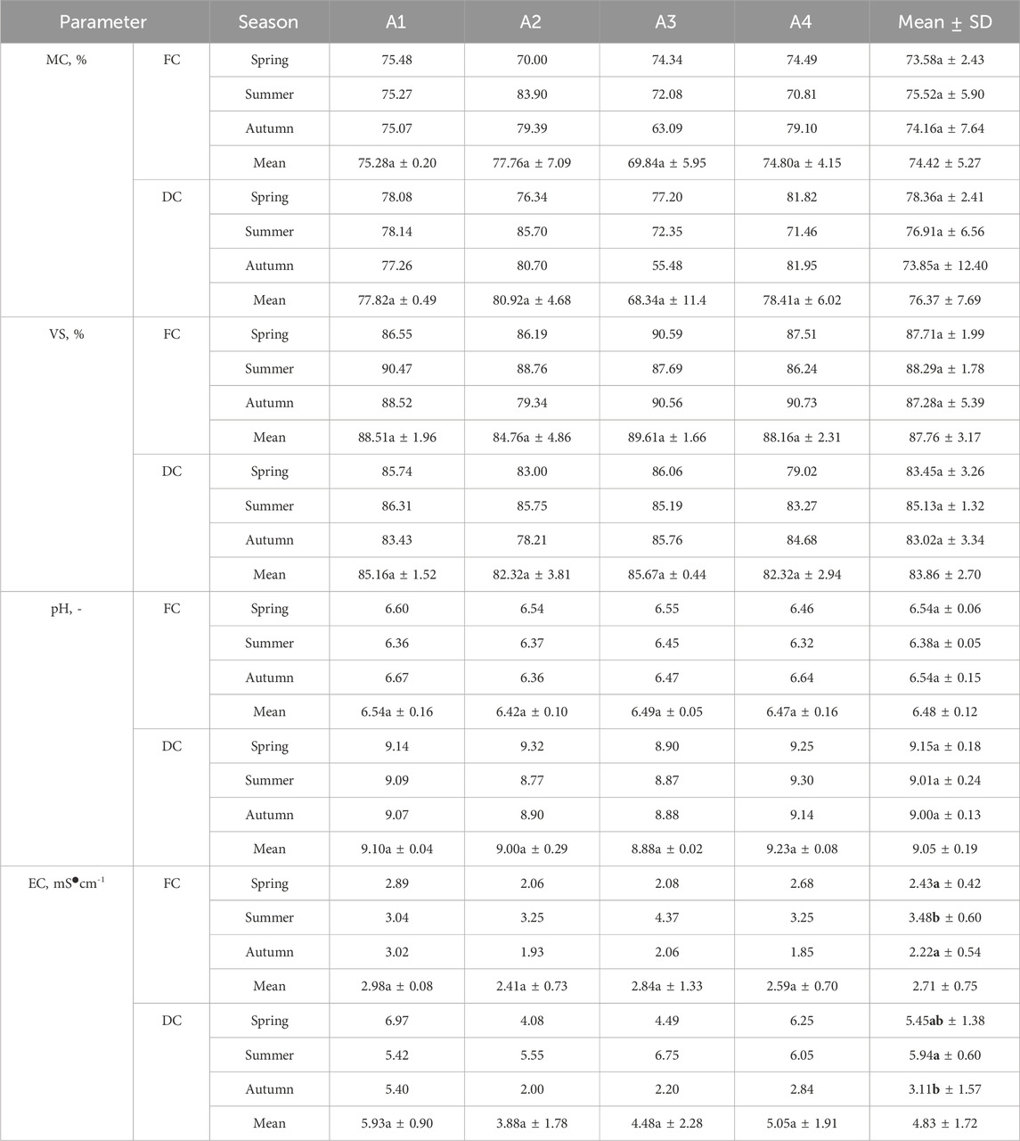
Table 3. Properties of fresh (FC) and decomposed clippings (DC) depending on the season and type of football pitch. Bold font highlights statistical significance.
The MC for fresh clippings was 74.42%, with the arithmetically lowest observed in the spring – 73.58%. Throughout football season, the arithmetically lowest average MC was on the A3 pitch (69.84%) and the arithmetically highest on the A2 pitch – 77.76%. The 14-day decomposition arithmetically increased the average MC to 76.37%. The MC arithmetically increased except for field A3 in the autumn (arithmetically decreased from 63.09% to 55.48%).
The average VS in all fresh samples was 87.76% ± 3.17% and was the arithmetically highest in summer (88.29%) (Table 3). Throughout the football season, fresh clippings from the A3 field had the highest VS (89.61%) followed by those from the A2 field (84.76%). The decomposition arithmetically decreased to the average VS level to 83.86%. The highest VS reduction was observed in the clippings from field A4 (from 88.16% to 82.32%).
Decomposition changed the pH of grass clippings from acid to alkaline. The mean pH increased from 6.48 to 9.05. The pH of fresh grass clippings throughout the football season was relatively stable and ranged from 6.32 to 6.67 (Table 3). The arithmetically highest mean value was observed for clippings obtained from the A1 pitch (6.54) and the arithmetically lowest for clippings from the A2 pitch (6.42). The arithmetically highest pH was observed for clippings from the A4 pitch, characterized by a low level of maintenance (9.23). Regarding the seasons, the decomposed grass clippings from the spring season had the highest average pH (9.15, while the decomposed clippings from the summer and autumn were arithmetically lower (9.00–9.01).
High EC variability was noted (Table 3). The fresh clippings EC ranged from 1.85 to 4.37 mS∙cm-1 (average of 2.71 mS∙cm-1). Decomposition increased EC in all samples (average of 4.83 mS∙cm-1). It is worth noting, however, that the change in EC with decomposition varied. For example, the EC in autumn cuttings obtained from the A2 field increased arithmetically by 0.07 mS∙cm-1 while, in the case of spring cuttings obtained from pitch A4, it increased by 3.57 mS∙mS∙cm-1. Statistical analysis showed that fresh and decomposed clippings were not statistically different in terms of pitch type, but statistically significant differences occurred in terms of seasonality.
The C, H, and N content was reduced during decomposition (Table 4). The statistical analysis showed significant differences between fresh and decomposed grass clippings from pitch A1 between C, H and N contents. Differences were not detected only for the C:N. No statistically significant differences were detected between any parameters for pitch A2 and A3. In contrast, for unfertilized clippings coming from pitch A4, statistically significant differences between fresh and decomposed clippings were observed only for the C:N parameter.
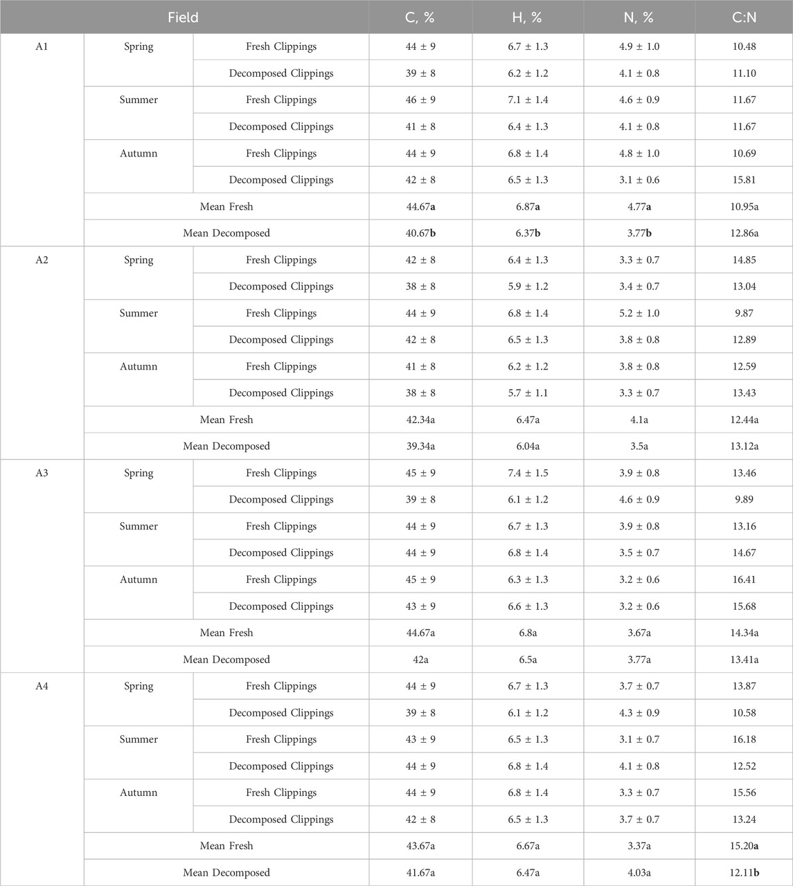
Table 4. Ultimate analysis of fresh and decomposed clippings depending on the season and type of football pitch. Bold font highlights statistical significance.
In general, the average C in fresh clippings ranged from 41% to 46%, the H from 6.2% to 7.4%, and N from 3.1% to 5.2%. The N content in fresh clippings was consistent with the fertilization level. In the case of highly fertilized A1 football turf, the average N was 4.76%, followed by A2 (4.10%), A3 (3.66%), and A4 (3.36%). The average C:N in fresh clippings from all football fields was 13.23 and was the highest for clippings obtained in the autumn season (13.81). In general, the average C:N ratio in fresh clippings was 13.23, and 12.88 in decomposed.
3.2 Respirometry activity and kinetics
Respiratory activity and the kinetics of the evaluated grass clippings showed high variability, depending on the season and their origin (Figure 3). Statistical analysis showed that there were no statistically significant differences between the seasons for cuttings from high-fertilized pitches (A1 and A2). For clippings coming from pitch A3, statistically significant differences were detected between spring and the other seasons. For unfertilized clippings coming from pitch A4, statistically significant differences were detected between the spring and summer seasons. In most cases, the highest AT4 values were observed in the autumn or spring and the lowest in the summer. In general, the average AT4 content (from all seasons) was the highest for highly fertilized A1 turf (253.2 mg O2∙g-1 d.m.), followed by a turf with an intermediate fertilization level (237.5 mg O2∙g-1 d.m.), non-fertilized A4 turf (237.0 mg O2∙g-1 d.m.), and A3 turf with low level of N fertilization (216.4 mg O2∙g-1 d.m.).
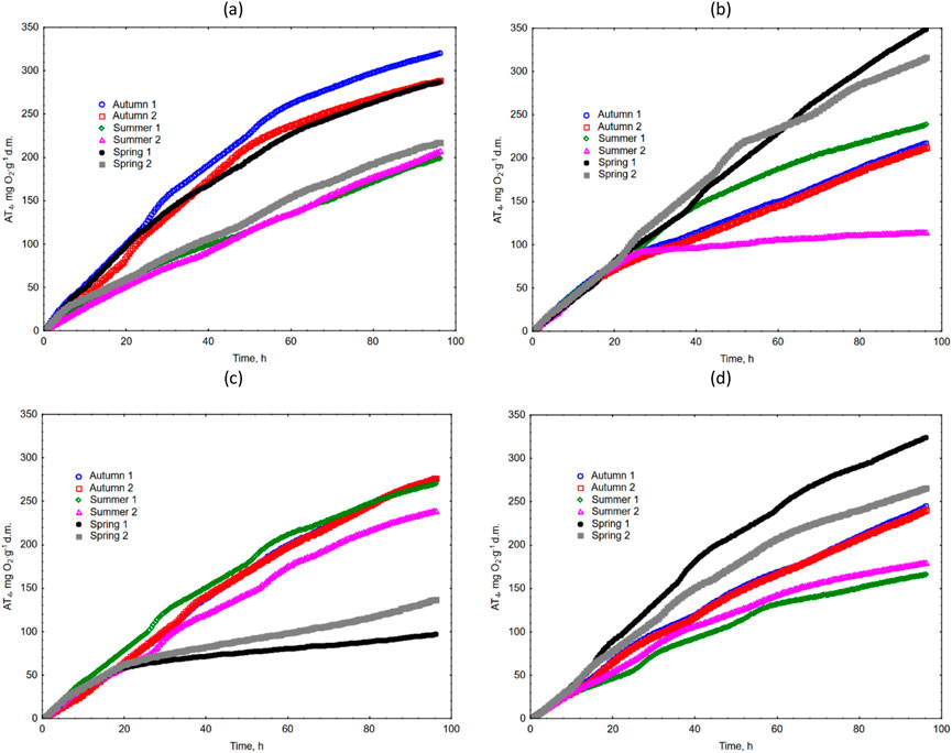
Figure 3. The respirometry activity (AT4) of grass clippings for (a) A1 turf; (b) A2 turf; (c) A3 turf; (d) A4 turf.
Kinetic constant rate k ranged from 0.00393 h-1 to 0.04522 h-1, and r ranged from 2.8831 mg O2⋅g-1 d.m.⋅h-1 to 6.3342 O2⋅g-1 d.m.⋅h-1 (R2 ranged from 0.967 to 0.999, Table 5). The kinetics was the fastest in spring (k = 0.016517 h-1) and slowed as the growing season progressed (summer k = 0.009853 h-1, autumn k = 0.009841 h-1). Regarding fertilization effect, the reaction kinetics was on average the fastest on the A3 turfs (k = 0.016592 h-1), and relatively similar for the other variants (k in the range of 0.009942 h-1 – 0.010458 h-1). Statistical analysis showed that there were no statistically significant differences between seasons for the k and r parameters for the cuttings from the A1 and A3 pitches (no statistical analysis was performed for the A2 and A4 pitches due to the inability to determine some of the k and r parameters).
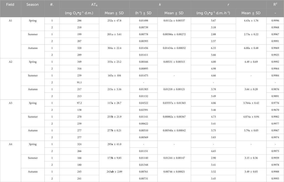
Table 5. Kinetics parameter of respiration activity for clippings depending on the season and type of football pitch. Bold font highlights statistical significance.
3.3 CO emissions
Cumulative CO emissions are shown in Figure 4. Detailed data are summarized in Supplementary Table S1. The lowest emission was from the summer clippings. The CO emission was <100 µg CO∙g-1 d.m. at the end of each trial. In the case of highly fertilized A1 turf, the highest CO emission was observed from the clippings from the autumn, where after 14 days, the cumulative emission was 456 µg CO∙g-1 d.m. Spring clippings from this turf had a cumulative emission of 286 µg CO∙g-1 d.m. A reverse trend was observed for the remaining three turfs (A2-A4), i.e., higher emissions than autumn characterized clippings from the spring. The most remarkable differences were noted in CO emissions from an average fertilization (A2) and the non-fertilized turfs (A4), where the average spring emissions ranged from 533 to 602 µg CO∙g-1 d.m., and 270 to 228 µg CO∙g-1 d.m. in the autumn, respectively. For A3, the difference in spring and autumn emissions was smaller, and ranged from 202 µg CO∙g-1 d.m. to 181 µg CO∙g-1 d.m., respectively.
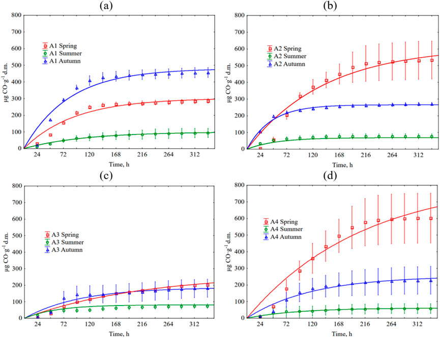
Figure 4. Cumulative CO production during grass clipping decomposition depends on the season and type of football pitch. The error bars show +/− standard deviation around the mean. The equations used in the figures are shown in Supplementary Table S2. (a) A1 turf; (b) A2 turf; (c) A3 turf; (d) A4 turf.
The seasonality of CO emissions for clippings from all types of pitches was characterized by a statistically significant changes, except for A3 pitch in spring and summer. The effect of fertilization was also significant in the CO emission. In spring, statistically significant differences were not observed only between variants A2 and A4, and in autumn - only between variants A3 and A4 (low-fertilized and non-fertilized turf). A slightly different situation was observed in the summer, where statistically significant differences in CO emissions were noted between highly fertilized turfs (A1 and A2) and non-fertilized turf (A4). Tables 6, 7 show detailed statistical analysis.
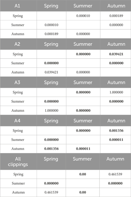
Table 6. Results of Kruskal-Wallis tests of the influence of seasonality on CO emission. Results in bold indicate statistically significant differences.
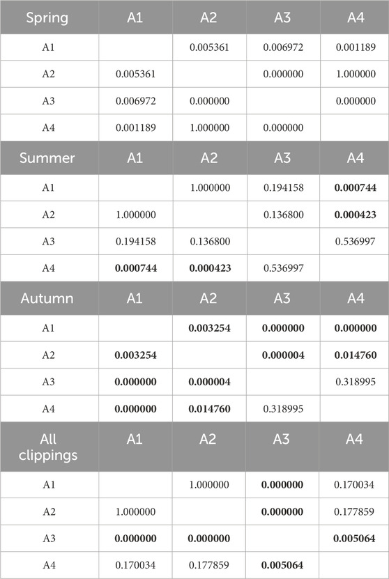
Table 7. Results of Kruskal-Wallis tests of the influence of fertilization level on CO emission. Results in bold indicate statistically significant differences.
3.4 CO2 emissions and O2 consumption
Cumulative CO2 emissions are shown in Figure 5. Detailed data is summarized in Supplementary Table S2. In most cases (clippings from A2-A4 turfs), the highest emissions occurred during decomposition of spring clippings. The highly fertilized turf (A1) was an exception, where the CO2 emissions from the autumn clippings (562 mg CO2∙g-1 d.m.) exceeded the spring ones (503 mg CO2∙g-1 d.m.). CO2 emission from A1 clippings in the summer was slightly lower (376 CO2∙g-1 d.m.). Generally, for the spring, the higher the level of N fertilization, the lower the CO2 emission (503, 638, 665, and 745 CO2∙g-1 d.m., from A1, A2, A3, A4 turfs, respectively). However, this trend did not occur in the later seasons. For summer, for the clippings from turfs treated with fertilizer (A1-A3), emitted 476, 494, and 558 CO2∙g-1 d.m., respectively. The CO2 emission for clippings from non-fertilized turf was relatively low (283 CO2∙g-1 d.m.). The summer clippings had the lowest average CO2 emissions compared to the spring and autumn seasons (similarly to the CO emissions pattern). In the autumn, the clippings from A4 non-fertilized turf were characterized by the highest CO2 emissions potential. In contrast, emissions the remaining turfs were very similar and amounted to 562, 557, and 557 CO2∙g-1 d.m., for A1 to A3 turfs, respectively. Statistical analyses showed that the level of fertilization has little effect on CO2 emissions. Statistically significant differences were observed only in summer between the clippings from non-fertilized A4 turf and other pitches. Tables 8, 9 show detailed statistical analysis for CO2 production.
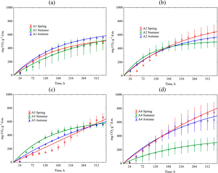
Figure 5. Cumulative CO2 production during grass clipping decomposition depends on the season and type of football pitch. The error bars show +/− standard deviation around the mean. The equations used in the figures are shown in Supplementary Table S4. (a) A1 turf; (b) A2 turf; (c) A3 turf; (d) A4 turf.
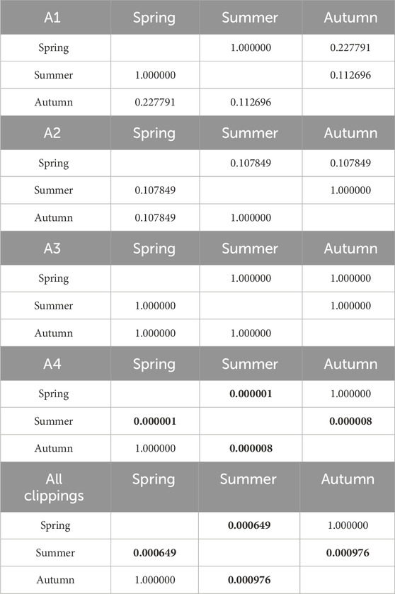
Table 8. Results of Kruskal-Wallis tests of the influence of seasonality on CO2 emission. Results in bold indicate statistically significant differences.
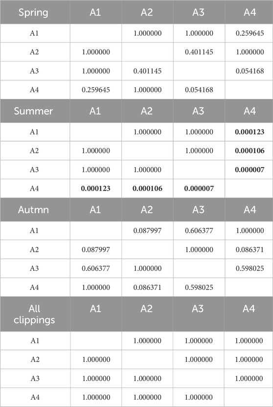
Table 9. Results of Kruskal-Wallis tests of the influence of fertilization level on CO2 emission. Results in bold indicate statistically significant differences.
Cumulative O2 consumption is shown in Figure 6. Detailed data is summarized in Supplementary Table S3. The process kinetics was similar to that of CO2 production. The lowest consumption occurred in the summer season (219 O2∙g-1 d.m. for A4, and 359, 376, and 426 O2∙g-1 d.m., for A1, A2, A3 turfs, respectively). For other seasons, the highest O2 consumption characterized clippings from non-fertilized A4 turf (spring, 580 O2∙g-1 d.m., and 395, 495, and 527 O2∙g-1 d.m., for A1, A2, and A3, respectively). As in the case of CO2 emissions, the lower N fertilization, the greater the O2 consumption was observed. In autumn, clippings from the non-fertilized A4 turf had O2 consumption of 463 O2∙g-1 d.m., while clippings from the remaining (A1-A3) pitches had a lower O2 consumption, ranging from 405 to 408 O2∙g-1 d.m. The effect of fertilization on O2 consumption was statistically insignificant in autumn and spring, but statistically significant in summer. The effect of season on O2 consumption was statistically significant only for the unfertilized football field (A4). Tables 10, 11 contain detailed information on the statistical analysis for O2 consumption.
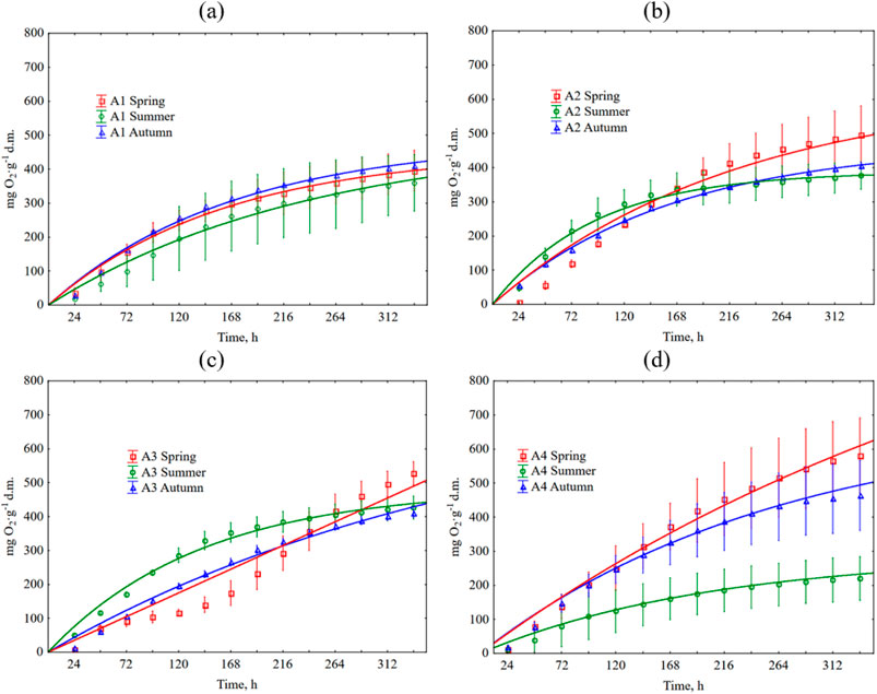
Figure 6. Cumulative O2 consumption during grass clipping decomposition depends on the season and type of football pitch. The error bars show +/− standard deviation around the mean. The equations used in the figures are shown in Supplementary Table S6. (a) A1 turf; (b) A2 turf; (c) A3 turf; (d) A4 turf.
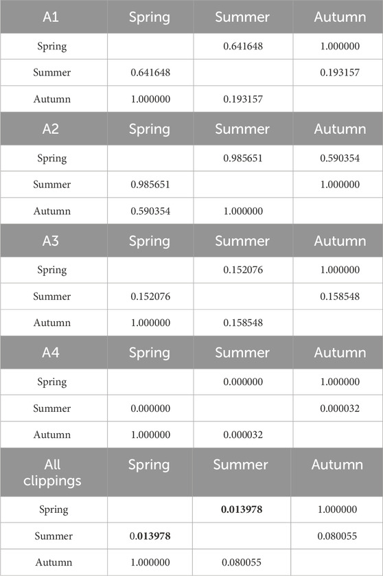
Table 10. Results of Kruskal-Wallis tests of the influence of seasonality on O2 consumption. Results in bold indicate statistically significant differences.
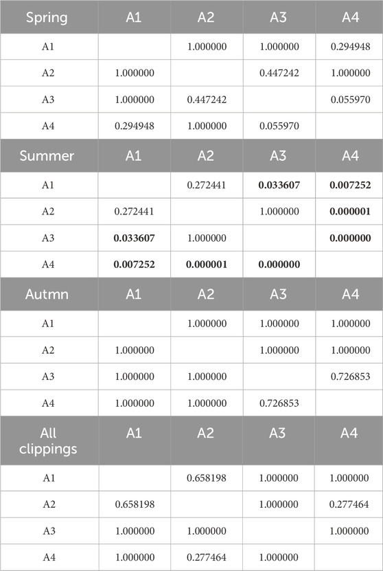
Table 11. Results of Kruskal-Wallis tests of the influence of fertilization level on O2 consumption. Results in bold indicate statistically significant differences.
3.5 Kinetics of CO, CO2 emissions, and O2 consumption
Tables 10, 11 contain detailed information on the statistical analysis for O2 consumption. Supplementary Tables S2, S4, S6 show the kinetic parameters of the models used to estimate CO and CO2 emissions and the consumption of O2. In all cases, the first-order kinetics model showed higher R2 than the 0-order model. However, in two instances, i.e., CO2 emission and O2 consumption for the A3 spring variant, it was decided to use the 0-order model with a slightly lower coefficient of determination due to the high discrepancy between the samples. Future mathematical modeling should include elements of environmental factors that may affect the decomposition of organic matter, e.g., the ambient temperature. This parameter can fluctuate greatly during the football season, thus affecting the shift in the proportion of a particular type of bacteria (psychrophilic, mesophilic, thermophilic), which can significantly affect CO, CO2 and O2 consumption (Stegenta-Dąbrowska et al., 2020). In addition, future mathematical models should include longer organic matter decomposition times (larger datasets) to more effectively estimate emission and consumption kinetics.
3.6 Modeling CO2 and CO production
In summary, all ANN models effectively predicted CO2 and CO emissions. The ANN models demonstrate similar dependencies in the raw data (Figures 7a,c). The correlations and high set quality (with values greater than 0.81 for CO and 0.98 for CO2 as shown in Supplementary Table S4) confirm the effectiveness of these models in predicting CO based on CO2 and O2, and CO2 based on CO and O2. As all tested models proved to be effective (Figures 7b,d), it was preferable to use the model with the smallest number of hidden neurons, i.e., MLP 3-3-1. Overall, the ANN models displayed reasonable adaptation to the data; however, notable statistical errors were evident in both the assessment of network quality (Supplementary Table S7) and the modeling performed (Figures 7b,d). It was observed that the models performed better at lower CO emissions (up to 350 µg CO∙g-1 d.m.) where the raw data set was larger (Figure 7a). At higher CO emissions, a significant increase in variability was observed, limiting the ANN’s effectiveness to the initial stages of the process. A more comprehensive model is still required for the intensive decomposition phase, where theoretically higher CO emissions could be observed. In the case of CO2 emission predictions, the ANN model’s accuracy was much higher (>0.98) and observed errors were lower, even at high emissions (Figure 7d).
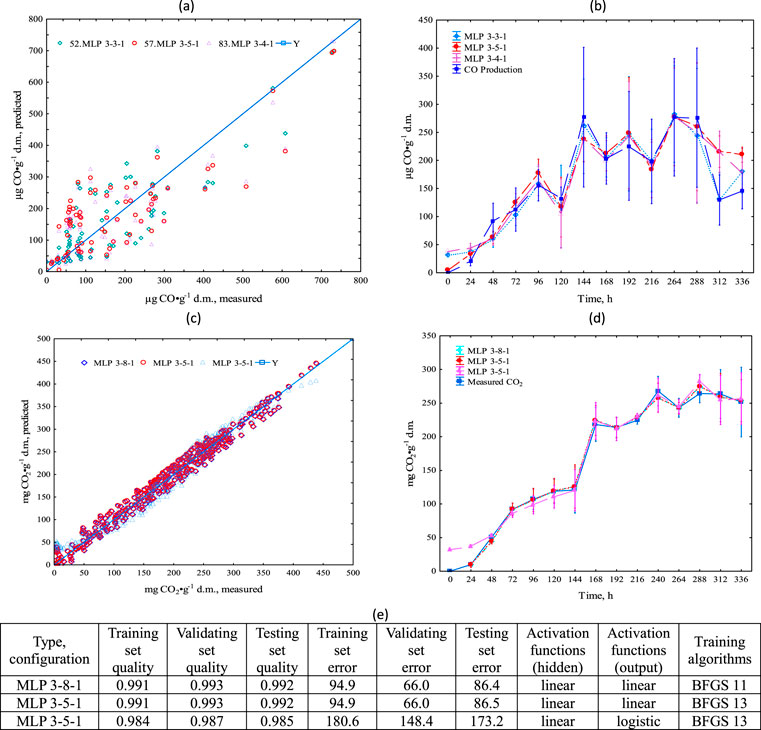
Figure 7. Process simulation with the neural network model–comparison of predicted and measured CO and CO2 production, (a) CO production in a time, (b) for entire dataset comparison of MLP 3-3-1, MLP 3-4-1, MLP, 3-5-1 for CO predictions, (c) CO2 production in a time, (d) for entire dataset comparison of MLP 3-3-1, MLP 3-4-1, MLP, 3-5-1 for CO2 predictions, (e) ANN statistical characteristics; mean ± standard error.
3.7 Key points from the supplementary materials
In Supplementary Tables S1–S6, we included models and parameters for the kinetic models shown in Figures 4–6. The mathematical models for CO production had an R2 range of 0.91–0.99, for CO2: 0.94–0.99, and for O2 consumption: 0.93–0.99. We have also included in the section ANN configurations for the MLP model and loads scattering plot from PCA analysis.
4 Discussion
4.1 Grass clippings properties
The average MC observed in fresh grass clippings (74.42%) should be considered typical observed on average over the growing season for various species and varieties of turf grasses. This was confirmed by the research of Kauer et al. (2012), who, by evaluating the MC in grass clippings from different periods, which additionally differed significantly in terms of N fertilization, reported MC ranging from 71.3% to 85.7%. Similar MC in grass clippings (73.40%), is a frequent assumption of the average throughout the growing season for various technical and economic analyzes (Sobol et al., 2021; Leible et al., 2015).
The average OM content of 87.76% in grass clippings was consistent with the previous research, i.e., 85.46%–88.34% (Leible et al., 2015; Nitsche et al., 2017), and was similar to the clippings from roadside verges (82.1%–93.11%) (Brown et al., 2020; Obernberger et al., 2006; Piepenschneider et al., 2016). The measured pH and EC did not differ significantly from those found in the literature (Olakanye et al., 2015; Zahrim et al., 2016). The grass clippings had a slight MC increase (∼2–3%) with very few exceptions. The process temperature (20 °C) may suggest that water was generated as a result of the progressing OM decomposition (Stegenta-Dąbrowska et al., 2020; Mason, 2006; Sobieraj, 2017; Wetzel et al., 2017).
The decrease in VS content can be explained by the OM loss due to microbiological degradation (Kalamdhad et al., 2012). A slight OM reduction in all cases could be due to the fact that all collected clippings were characterized by a similar initial OM content and MC, hence the decomposition level was also similar (Stegenta-Dąbrowska et al., 2020; De Guardia et al., 2008). In the context of decomposition of grass clippings left on the soil, it has been shown that their decomposition occurs most quickly in high air humidity and temperature up to 10 °C, beyond which the decomposition rate decreases, which may explain a slight decrease in the OM content (Kauer et al., 2012).
However, it is worth adding that this temperature is exceeded in most months of the grass growing season in Polish climate conditions, hence the experiment was carried out at a constant temperature of 20 °C (Talar-Krasa et al., 2021). In addition, because the process provided optimal conditions with regard to the O2 content, the pH of grass clippings increased due to decomposition, as is the case with composting (Soto-Paz et al., 2019; Wang et al., 2016; Waqas et al., 2018).
As expected, a higher N level was observed in grass clippings from sports turf treated with a high dose of N fertilizer. This is consistent with the literature, where increasing the N fertilization rate increases N content in clippings (Grégoire et al., 2022). Our experiment also showed the importance of season. The importance of these two factors is also confirmed by Shaddox and Unruh (2018), who report that many factors may influence turfgrass uptake of N, including turfgrass species, season, N type, N rate, and MC management. On the other hand, the obtained C:N ratio of fresh grass clippings were relatively low; however, they were within the standard range, which is 12–25, according to Singh and Longkumer (2018). The 2-week process of decomposing grass clippings resulted in a percentage decrease in N content in some samples; this phenomenon was especially noticeable in the case of clippings obtained from highly fertilized turfs (A1 and A2). This could be caused by NH3 volatilization and leaching (Ansari and Rajpersaud, 2012). On the other hand, in the case of turf fertilized with a low N dose (A3) and non-fertilized turf (A4), a negative percentage change was observed, which can probably be explained by microbiological utilization (Ansari and Rajpersaud, 2012).
This experiment showed a reduction in C content, which is often an indicator of enhanced decomposition (Ansari and Rajpersaud, 2012; Agrawal et al., 2011; Rahul, 2011; Sharma et al., 2003; Stoffella and Kahn, 2001). On average, a slightly higher C reduction was obtained for grass clippings obtained from highly fertilized turfs (A1 and A2). This may indicate that the fertilization level affects the rate of clippings decomposition, but on the other hand, the level of C reduction was relatively similar between treatments, hence the need for further research to explain this phenomenon.
AT4 was higher than those for grass clippings reported in the literature, i.e. (Godley et al., 2004), 119 mg O2∙g-1 d.m (Stegenta-Dąbrowska et al., 2020), 188 mg O2∙g-1 d.m, and (Suchowska-Kisielewicz and Jędrczak, 2019) 162 mg O2∙g-1 d.m. Likely, these differences were due to a wide range of grass species and varieties, habitats and conditions, diverse chemical composition and heterogeneous structure (Waliszewska et al., 2021). These aspects are often overlooked when describing the substrate origin but can have an impact on microorganisms and the decomposition of grass clippings. Based on the results, it can be concluded that the level of N fertilization was not a factor that strongly influences the respiratory activity. Initially, it can be assumed that the season plays a much greater role. However, readers should be aware that between samples it was sometimes possible to observe large fluctuations between results, as exemplified by the A2 grass clippings sample from the summer season. All mathematical models used to describe the AT4 were first-order and were characterized by a high R2 (>0.967), which is typical for modeling the kinetics of the respiratory activity process (Stegenta-Dąbrowska et al., 2020). The r constant, apart from a few outliers, were comparable with the Fernández et al. (2008) studies, with r values ranging from 0.0009 to 0.0018 h-1.
4.2 CO, CO2 production and O2 consumption during clippings decomposition
To date, managed grass surfaces were considered in the context of CO2 emissions and in relation to biogenic CO2 emissions (the effect of mowing grass on soil respiration) and anthropogenic CO2 emissions (emissions resulting from the use of gasoline for mower engines) (Lerman and Contosta, 2019). In this research, the seasons and fertilizer amount did not have a significant effect for microorganism activity as a production of CO2 (Figure 5). In turf A4 (no fertilization), the effect of the seasons was clear–the highest activity was observed in spring and the least in summer. This could be explained by C:N ratio, e.g., the A4 C:N ratio was the most optimal for decomposition of biodegradable OM. The ideal range for the C:N ratio varies from 15 to 30, while composting can have a broader range of values. According to Ba et al. (2020), the total C and N contents are the key variables impacting CO2 emissions because greater C and N contents are more favorable to microorganism respiration. This was clearly visible only on A4 turf. Bai et al. (2020) observed that addition of lignite reduced N losses, but increased CO2 emissions, i.e., the total GHG emissions from the lignite-amended manure were 2.6 times greater than that of the non-lignite treatment. This means that variants with fertilization (A1, A2 and A3) with low C content, have less CO2 emissions, which was observed in this research.
Influence of biomass type decomposition on OM has been widely studied by Montejo et al. (2015) who confirmed that materials with optimal range of nutrients effect the quality of compost. Temperature, humidity, pH, aeration and C:N ratio are important in the process of aerobic degradation (Martínez-Valdez et al., 2015), facilitating fast biodegradation and lower impact on environment in terms of gaseous emissions and leaching. In this study we did not observe this, which could possibly be explained by pesticide use, which is known to strongly affect microbiological consortia in soil and grass. Pesticides could remain in the environment, affecting long-term changes in the microbial community. Overall, our results suggest that the pesticide application might affect the soil C cycle and may disrupt the formation of soil OM and structure stabilization (Sim et al., 2022).
All the analyzed variants showed low CO emissions during the summer (Figure 4), regardless of the applied fertilization. High summer temperatures could induce thermochemical production of CO, still on the football fields; hence the CO emissions during incubation at 20 °C were low. As recent research by Sobieraj (2025) has shown, higher temperatures intensified CO production, which is an important finding in the context of our work, because in the summer season, the air temperature can be higher than 20 °C, at which the experiment was conducted. The author also emphasizes the need to conduct research on different moisture content levels in substrates, which may also yield interesting findings regarding the impact of irrigation systems on CO emissions in future studies.
However, in comparison with our previous CO emissions report (Stegenta-Dąbrowska et al., 2020) from mixture of grass and cow manure, total CO emission in this experiment was even 5 times higher. This is also confirmed by the results of biological activity (AT4 index in Figure 3) which were the lowest in the variants from the summer. These differences are visible, especially in the variant without fertilization. On average, 0.26 mg CO⋅g-1 d.m. was emitted from the decomposition process (Table 12) which is higher in relation to grass composting (∼0.11 mg CO⋅g-1 d.m.), but still a small value compared to CO emissions from open burning of the grasslands (59 mg CO⋅g-1 d.m.). Nevertheless, grass decomposition can contribute significantly to global CO emissions.

Table 12. Emission factors for processes involving grass.
Differences in CO emissions are not clearly related to the level of fertilization, season, or C and N content. Also, the amount of available N in the form of NO3−, or simple indicators such as pH or EC, do not have an apparent effect on the amount of CO. Although Conrad and Seiler (1985) clearly indicated the impact of these parameters on emissions. However, the CO production is a very complex process and the net produced is the result of both the consumption and utilization by microorganisms in various metabolic pathways (Sobieraj et al., 2022; Sobieraj et al., 2023). On the other hand, the fertilized turfs (A1, A2, A3), were also sprayed several times with different herbicides. Herbicides could significantly change the composition of the local microflora (Ruuskanen et al., 2023), also contributing to the observed net CO emissions. The observed highest CO emission (A4 variant) confirms our previous results (Stegenta-Dąbrowska et al., 2019) that the amount of CO is a product of the thermochemical and biological pathways, and the disturbance of one of these processes leads to lower CO emissions, but these emissions are then very difficult to predict if based solely on the compost composition itself.
Another possible explanation of the observed differences in CO emissions is that different fertilization levels may have resulted in different soil microflora (Liu et al., 2022; Ren et al., 2020). The varietal composition of the grass itself might be a factor. Future studies explaining the causes of CO emissions from grass clippings should also include microbiological tests, for developing the microbiome. Recent studies indicate that identifying the specific bacteria responsible for CO release and analyzing their metabolic pathways can help understand CO production in similar biological processes (Sobieraj et al., 2025; Sobieraj et al., 2024). Hence, we propose that this is the next step in researching CO emissions from sports turf. Given that both pesticide/herbicide application and fertilization levels could have significantly affected the dynamics of the microflora and the dynamics of changes in its community (Figure 8), microbiological tests can greatly facilitate the interpretation of CO production variability.
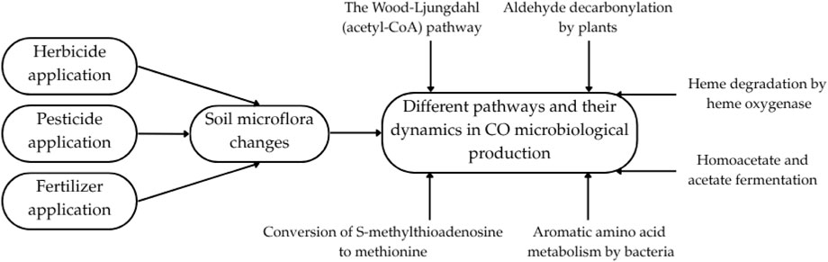
Figure 8. Potential change in soil microflora through the application of pesticides/herbicides/fertilizers and its impact on the dynamics of microbiological CO production pathways. Microbiological CO production pathways were used from Sobieraj et al. (2023).
4.3 Prediction of CO2 and CO production
Given the substantial amount of CO and CO2 emissions produced during storing of grass clippings, it is reasonable to predict these emissions in this process. There have been limited studies on the application of AI - machine learning (ML) models - for emissions prediction during the storage or composting of organic waste thus far. Common ML models used in composting are as follows: Random Forest (RF), ANN, Support Vector Regression (SVR), Decision Tree, and Decision Support (DS) (Temel et al., 2023). The majority of studies primarily address CO2 and NH3 emissions, with little attention given to predicting CO emissions, which have been found to exceed those produced in conventional composting methods. The utility of ANN in developing accurate emission prediction models was a key factor in its utilization for this study.
The performance of machine learning (ML) models utilized for predicting composting processes exhibited a variance in R-squared (R2) accuracy ranging from 0.56 to 0.99 (Temel et al., 2023). However, the majority of cases demonstrated a strong fit, with R2 values exceeding 0.7. In this study, the obtained R-squared value for the ANN exceeded 0.8.
5 Limitations and recommendations for future plot experiments
Because the nature of our work involved grass clippings, harvested from the real football fields, we could not control several parameters - including soil type, irrigation frequency, fertilizer frequency, or the use of a uniform mix of grass species. In addition, some operators admitted to using pesticides, which may have affected the results to some extent. The use of different agronomic treatments at different times also may have distorted the distinction of seasonal effects on the emissions studied. It is also worth mentioning that grass surfaces were mowed with different mowers, so that the shredded levels of grass clippings were also diversified. Moreover, the species composition of grasses on the turf is constantly evolving and changing, so we were not able to monitor their changes throughout the football field. Furthermore, it should be acknowledged that while this article has endeavored to choose a variety of turf surface types with varying management levels, there are likely pitches with entirely different management systems, which may also influence the outcomes on a larger scale. The management practices of the pitches analyzed in the article are characteristic of the Lower Silesia region in Poland. Thus, it is imperative to pursue further research in this domain to optimize the utilization of the findings obtained from this study.
Although we have observed preliminary trends and the effects of some parameters on emissivity (such as pH), in order to distinguish the effect of fertilization on CO and CO2 emissions from grass clippings decomposition, we propose that future work should focus on experimental plots. Conducting experiments on experimental microplots, along with setting up plots on the same technical parameters - soil type, size and frequency of irrigation, same grass mixture, limiting the use of other chemicals (pesticides/herbicides), using the same agrotechnical equipment - will allow better control of the experiment. Better control of parameters and observation of potential changes in the species composition of grasses will make it possible to better distinguish the direct effect of fertilization and seasonality on emissivity from the decomposition of grass clippings. As we also mentioned in the discussion, microbiological tests seem to be the next critical step that could link the dynamics of microflora and its impact on CO production. The results generated can significantly contribute to emission inventories and CO/CO2 estimates from other types of sports surfaces and urban lawns. Future work should also evaluate other types of surfaces, such as golf courses and rugby fields, where management is quite different from football fields and the scale of grass generated is larger. Consequently, their GHG budget is different (Kuronuma et al., 2023). To get a better understanding of this phenomenon, it may also be helpful to check the physicochemical characteristics of the turf prisms (pH, humidity, temperature) and adjust the parameters of the decomposition process on this basis.
6 Conclusion
Determination of environmental impacts resulting from the decomposition of grass clippings after mowing sports turfs and grass surfaces is needed to enable the quantification and estimation of gaseous emissions and to ensure the safety of football players, fans, and field operators. This lab-scale experiment showed that the decomposition of grass clippings can generate significant CO emissions, i.e., up to 5 times more than in previous experiments for a mixture of grass and cow manure. However, a high diversification of results was noted, from which the effect of fertilization, seasonality, C and N content on CO emission was not clearly distinguished. A similar lack of apparent relationships was observed in the context of CO2 emissions and O2 consumption. Initial models ANN have successfully predicted the CO and CO2 emissions resulting from the disposal of grass clippings. The models demonstrate satisfactory outcomes with R2 accuracy: CO > 0.81 and CO2 > 0.98. More research is needed to account for CO emissions from decomposing biomass such as common grass clippings and improvement of emission inventories of primary pollutants such as CO. More scaled up work is needed (pilot and then full-scale), to elucidate the effects of season, turf type, and management technology on CO/CO2 emissions to provide best practice recommendations for municipal turf managers and waste handlers.
Data availability statement
The original contributions presented in the study are included in the article/Supplementary Material, further inquiries can be directed to the corresponding author.
Author contributions
ŁS: Data curation, Formal Analysis, Investigation, Methodology, Resources, Software, Visualization, Writing – original draft. JK: Validation, Writing – review and editing. SS-D: Conceptualization, Data curation, Formal Analysis, Methodology, Project administration, Resources, Software, Supervision, Validation, Writing – original draft, Writing – review and editing.
Funding
The author(s) declare that financial support was received for the research and/or publication of this article. This work was supported by the Wrocław University of Environmental and Life Sciences (Poland) as part of the research program “Young Minds”, N010/0001/21”.
Acknowledgments
The authors would like to thank the following football clubs that made the research possible - Pogoń Oleśnica, KP Śliwice, Dąb Dobroszyce. The authors would like to thank Zenon Olewiński and Jarosław Sobol for special administrative assistance and making grass clippings available.
Conflict of interest
The authors declare that the research was conducted in the absence of any commercial or financial relationships that could be construed as a potential conflict of interest.
Generative AI statement
The author(s) declare that no Generative AI was used in the creation of this manuscript.
Any alternative text (alt text) provided alongside figures in this article has been generated by Frontiers with the support of artificial intelligence and reasonable efforts have been made to ensure accuracy, including review by the authors wherever possible. If you identify any issues, please contact us.
Publisher’s note
All claims expressed in this article are solely those of the authors and do not necessarily represent those of their affiliated organizations, or those of the publisher, the editors and the reviewers. Any product that may be evaluated in this article, or claim that may be made by its manufacturer, is not guaranteed or endorsed by the publisher.
Supplementary material
The Supplementary Material for this article can be found online at: https://www.frontiersin.org/articles/10.3389/fenvs.2025.1632196/full#supplementary-material
References
Afzal, M., Agarwal, S., Rabab, H., Elshaikh, , Choudhary, R. K., Prabhakar, P. K., et al. (2025). Carbon monoxide poisoning: diagnosis, prognostic factors, treatment strategies, and future perspectives. Diagnostics 15 (5), 581. doi:10.3390/diagnostics15050581
Agrawal, P., Kumar, C., Prakash, A., and Devendra, C. (2011). Bacterial diversity in a bagasse-based compost prepared for the cultivation of edible mushrooms Agaricus bisporus 7, 2103–2111.
Akagi, S. K., Yokelson, R. J., Wiedinmyer, C., Alvarado, M. J., Reid, J. S., Karl, T., et al. (2011). Emission factors for open and domestic biomass burning for use in atmospheric models. Atmos. Chem. Phys. 11 (9), 4039–4072. doi:10.5194/acp-11-4039-2011
Al-Wabel, M. I., Abdulrasoul, A.-O., El-Naggar, A. H., Nadeem, M., and Usman, A. R. A. (2013). Pyrolysis temperature induced changes in characteristics and chemical composition of biochar produced from conocarpus wastes. Bioresour. Technol. 131, 374–379. doi:10.1016/j.biortech.2012.12.165
Ansari, A. A., and Rajpersaud, J. (2012). Physicochemical changes during vermicomposting of water hyacinth (Eichhornia Crassipes) and grass clippings. ISRN Soil Sci. 2012, 1–6. doi:10.5402/2012/984783
Ba, S., Qu, Q., Zhang, K., and Groot, i J. C. J. (2020). Meta-analysis of greenhouse gas and ammonia emissions from dairy manure composting. Biosyst. Eng. 193, 126–137. doi:10.1016/j.biosystemseng.2020.02.015
Bai, M., Impraim, R., Coates, T., Flesch, T., Trouvé, R., van Grinsven, H., et al. (2020). Lignite effects on NH3, N2O, CO2 and CH4 emissions during composting of manure. J. Environ. Manag. 271, 110960. doi:10.1016/j.jenvman.2020.110960
Binner, E., Böhm, K., and Lechner, P. (2012). Large scale study on measurement of respiration activity (AT4) by Sapromat and OxiTop. Waste Manage. 32, 1752–1759. doi:10.1016/j.wasman.2012.05.024
Boldrin, A., Andersen, J. K., Jacob, M., Christensen, T. H., and Favoino, E. (2009). Composting and compost utilization: accounting of greenhouse gases and global warming contributions. Waste Manag. and Res. J. a Sustain. Circular Econ. 27 (8), 800–812. doi:10.1177/0734242X09345275
Bremer, D. J. (2006). Nitrous oxide fluxes in turfgrass: effects of nitrogen fertilization rates and types. J. Environ. Qual. 35 (5), 1678–1685. doi:10.2134/jeq2005.0387
Brown, A. E., Ford, J. S., Bale, C. S. E., Camargo-Valero, M. A., Cheffins, N. J., Mason, P. E., et al. (2020). An assessment of road-verge grass as a feedstock for farm-fed anaerobic digestion plants. Biomass Bioenergy 138, 105570. doi:10.1016/j.biombioe.2020.105570
Cheng, Y., Bi, X., Xu, Y., Liu, Y., Li, J., Du, G., et al. (2023). Artificial intelligence technologies in bioprocess: opportunities and challenges. Bioresour. Technol. 369, 128451. doi:10.1016/j.biortech.2022.128451
Conrad, R., and Seiler, W. (1985). Influence of temperature, moisture, and organic carbon on the flux of H2 and CO between soil and atmosphere: field studies in subtropical regions. J. Geophys. Res. Atmos. 90 (D3), 5699–5709. doi:10.1029/jd090id03p05699
Dang, J., and Chou, K.-C. (2018). A model for the reduction of metal oxides by carbon monoxide. ISIJ Int. 58 (4), 585–593. doi:10.2355/isijinternational.ISIJINT-2017-630
De Guardia, A., Petiot, C., Rogeau, D., and Druilhe, C. (2008). Influence of aeration rate on nitrogen dynamics during composting. Waste Manag. 28 (3), 575–587. doi:10.1016/j.wasman.2007.02.007
Fernández, F. J., Sánchez-Arias, V., Villaseñor, J., and Rodríguez, L. (2008). Evaluation of carbon degradation during Co-Composting of exhausted grape marc with different biowastes. Chemosphere 73 (5), 670–677. doi:10.1016/j.chemosphere.2008.07.007
Follett, R., Mooney, S., and Morgan, J. (2011). Carbon sequestration and greenhouse gas fluxes in agriculture: challenges and opportunities.
Foresti, R., Bani-Hani, M. G., and Motterlini, R. (2008). Use of carbon monoxide as a therapeutic agent: promises and challenges. Intensive Care Med. 34 (4), 649–658. doi:10.1007/s00134-008-1011-1
Godley, A. R., Lewin, K., Graham, A., Barker, H., and Smith, R. (2004). Biodegradability determination of municipal waste: an evaluation of methods.
Grégoire, G., Benjannet, R., and Desjardins, Y. (2022). Contribution of grass clippings to turfgrass fertilization and soil water content under four nitrogen levels. Sci. Total Environ. 837, 155765. doi:10.1016/j.scitotenv.2022.155765
Grossi, N., Volterrani, M., Magni, S., and Miele, i S. (2004). Tall fescue turf quality and soccer playing characteristics as affected by mowing height. Acta Hortic. 661, 319–322. doi:10.17660/ActaHortic.2004.661.41
Haarstad, K., Bergersen, O., and Sørheim, i R. (2006). Occurrence of carbon monoxide during organic waste degradation. J. Air and Waste Manag. Assoc. 56 (5), 575–580. doi:10.1080/10473289.2006.10464470
Ignatieva, M., Haase, D., Dushkova, D., and Haase, A. (2020). Lawns in cities: from a globalised urban green space phenomenon to sustainable nature-based solutions. Land 9 (3), 73. doi:10.3390/land9030073
Ignatieva, M., Hughes, M., Chaudhary, A. K., and Mofrad, F. (2024). The lawn as a social and cultural phenomenon in Perth, Western Australia. Land 13 (2), 191. doi:10.3390/land13020191
Kalamdhad, A. S., Meena, K., and Absar, A. K. (2012). Drum composting of municipal solid waste. Environ. Technol. 33 (3), 299–306. doi:10.1080/09593330.2011.572918
Kauer, K., Raave, H., Köster, T., Viiralt, R., Noormets, M., Keres, I., et al. (2012). The decomposition of turfgrass clippings is fast at high air humidity and moderate temperature. Acta Agric. Scand. Sect. B - Soil and Plant Sci. 62 (3), 224–234. doi:10.1080/09064710.2011.602357
Kuronuma, T., Masuda, S., Mito, T., and Watanabe, H. (2023). Inclusive greenhouse gas budget assessment in turfs: from turf production to disposal of grass clippings. J. Environ. Manag. 346, 118919. doi:10.1016/j.jenvman.2023.118919
Law, Q. D., Trappe, J. M., Braun, R. C., and Patton, A. J. (2021). Greenhouse gas fluxes from turfgrass systems: species, growth rate, clipping management, and environmental effects. J. Environ. Qual. 50 (3), 547–557. doi:10.1002/jeq2.20222
Leible, L., Kälber, S., Kappler, G., Oechsner, H., and Mönch-Tegeder, M. (2015). Biogas aus Landschaftspflegegras: Möglichkeiten und Grenzen (KIT Scientific Reports; 7691). KIT Scientific Publishing. doi:10.5445/KSP/1000045983
Lerman, S. B., and Contosta, A. R. (2019). Lawn mowing frequency and its effects on biogenic and anthropogenic carbon dioxide emissions. Landsc. urban Plan. 182, 114–123. doi:10.1016/j.landurbplan.2018.10.016
Liu, H., Li, S., Qiang, R., Lu, E., Li, C., Zhang, J., et al. (2022). Response of soil microbial community structure to phosphate fertilizer reduction and combinations of microbial fertilizer. Front. Environ. Sci. 10, 899727. doi:10.3389/fenvs.2022.899727
March, S. R., Martins, D., and McElroy, J. S. (2013). Growth inhibitors in turfgrass. Planta Daninha 31 (3), 733–747. doi:10.1590/S0100-83582013000300025
Martínez-Valdez, F. J., Martínez-Ramírez, C., Martínez-Montiel, L., Favela-Torres, E., Soto-Cruz, N., Ramírez-Vives, F., et al. (2015). Rapid mineralisation of the organic fraction of municipal solid waste. Bioresour. Technol. 180, 112–118. doi:10.1016/j.biortech.2014.12.083
Mason, I. G. (2006). Mathematical modelling of the composting process: a review. Waste Manag. 26 (1), 3–21. doi:10.1016/j.wasman.2005.01.021
Montejo, C., Costa, C., and Márquez, M. C. (2015). Influence of input material and operational performance on the physical and chemical properties of MSW compost. J. Environ. Manag. 162, 240–249. doi:10.1016/j.jenvman.2015.07.059
Montgomery, B. (2009). Efficient and economical mowing. Sportsf. Manag. 35, 34–37. Available online at: https://sportsfieldmanagementonline.com/2019/10/01/efficient-and-economical-mowing/10760/.
Nitsche, M., Hensgen, F., and Wachendorf, M. (2017). Using grass cuttings from sports fields for anaerobic digestion and combustion. Energies 10 (3), 388. doi:10.3390/en10030388
Noer, O. J. (1945). Yield and chemical composition of clippings from a green of Washington bent grass. Golfdom 2, 13–16. Available online at: https://archive.lib.msu.edu/tic/golfd/article/1945feb13.pdf.
Obernberger, I., Brunner, T., and Barnthaler, G. (2006). Chemical properties of solid biofuels—significance and impact. Biomass Bioenergy 30 (11), 973–982. doi:10.1016/j.biombioe.2006.06.011
Olakanye, A. O., Thompson, T., and Komang Ralebitso-Senior, T. (2015). Shifts in soil biodiversity—A forensic comparison between sus scrofa domesticus and vegetation decomposition. Sci. and Justice 55 (6), 402–407. doi:10.1016/j.scijus.2015.07.004
Piepenschneider, M., Bühle, L., Frank, H., and Wachendorf, M. (2016). Energy recovery from grass of urban roadside verges by anaerobic digestion and combustion after pre-processing. Biomass Bioenergy 85, 278–287. doi:10.1016/j.biombioe.2015.12.012
Qian, Y., and Follett, R. F. (2002). Assessing soil carbon sequestration in turfgrass systems using long-term soil testing data. Agron. J. 94 (4), 930–935. doi:10.2134/agronj2002.9300
Rahul, K. (2011). Removal of pathogens during vermi-stabilization. J. Environ. Sci. Technol. 4 (6), 621–629. doi:10.3923/jest.2011.621.629
Ren, N., Wang, Y., Ye, Y., Zhao, Y., Huang, Y., Fu, W., et al. (2020). Effects of continuous nitrogen fertilizer application on the diversity and composition of rhizosphere soil bacteria. Front. Microbiol. 11, 1948. doi:10.3389/fmicb.2020.01948
Rosik, J., Maciej, K., and Stegenta-Dąbrowska, S. (2024). Optimizing the early-stage of composting process emissions – artificial intelligence primary tests. Sci. Rep. 14 (1), 27299. doi:10.1038/s41598-024-79010-0
Ruuskanen, S., Fuchs, B., Nissinen, R., Puigbò, P., Rainio, M., Saikkonen, K., et al. (2023). Ecosystem consequences of herbicides: the role of microbiome. Trends Ecol. and Evol. 38 (1), 35–43. doi:10.1016/j.tree.2022.09.009
Salman, A., and Avcioglu, R. (2010). Performances of some cool season turfgrasses in different fertilizer doses. Ege Üniv. Ziraat Fak. Derg. 47 (3), 309–319.
Schade, G. W., Hofmann, R.-M., and Crutzen, P. J. (1999). CO emissions from degrading plant matter: (I). Measurements. Tellus B Chem. Phys. Meteorology 51 (5), 889. doi:10.3402/tellusb.v51i5.16501
Shaddox, T. W., and Unruh, J. B. (2018). The fate of nitrogen applied to Florida turfgrass: ENH1282/EP546, 1/2018. EDIS 2018 (1). doi:10.32473/edis-ep546-2018
Sharma, S., and Sharma, S. (2003). Municipal solid waste management through vermicomposting employing exotic and local species of earthworms. Bioresour. Technol. 90 (2), 169–173. doi:10.1016/s0960-8524(03)00123-8
Sim, J. X. F., Drigo, B., Doolette, C. L., Vasileiadis, S., Karpouzas, D. G., and Lombi, E. (2022). Impact of twenty pesticides on soil carbon microbial functions and community composition. Chemosphere 307, 135820. doi:10.1016/j.chemosphere.2022.135820
Singh, R. K., and Longkumer, T. E. (2018). Compost: the black gold. KrishiVigyan Kendra–Phek, ICAR–NRC Mithun, Porba, Phek, Nagal. 112.
Sobieraj, K. (2017). Wykorzystanie pomiaru aktywności oddechowej Do wyznaczania zawartości Łatwo biodegradowalnej materii organicznej w odpadach. PRZEM. Chem. 1 (8), 112–115. doi:10.15199/62.2017.8.23
Sobieraj, K. (2025). Optimization of the organic matter content and temperature in a bioreactor to enhance carbon monoxide production during the initial phase of food waste composting. Molecules 30 (13), 2807. doi:10.3390/molecules30132807
Sobieraj, K., Stegenta-Dąbrowska, S., Koziel, J. A., and Białowiec, A. (2021). Modeling of CO accumulation in the headspace of the bioreactor during organic waste composting. Energies 14 (5), 1367. doi:10.3390/en14051367
Sobieraj, K., Stegenta-Dąbrowska, S., Luo, G., Koziel, J. A., and Białowiec, A. (2022). Carbon monoxide fate in the environment as an inspiration for biorefinery industry: a review. Front. Environ. Sci. 10, 822463. doi:10.3389/fenvs.2022.822463
Sobieraj, K., Stegenta-Dąbrowska, S., Luo, G., Koziel, J. A., and Białowiec, i A. (2023). Biological treatment of biowaste as an innovative source of CO—The role of composting process. Front. Bioeng. Biotechnol. 11, 1126737. doi:10.3389/fbioe.2023.1126737
Sobieraj, K., Derkacz, D., Krasowska, A., and Białowiec, A. (2024). Isolation and identification of carbon monoxide producing microorganisms from compost. Waste Manag. 182, 250–258. doi:10.1016/j.wasman.2024.04.044
Sobieraj, K., Żebrowska-Różańska, P., Siedlecka, A., Łaczmański, Ł., and Białowiec, A. (2025). Analysis of microbial community potentially involved in carbon monoxide production in compost and its functional assessment: utilized pathways, enzymes, and genes. Sci. Total Environ. 968, 178860. doi:10.1016/j.scitotenv.2025.178860
Sobol, Ł., Dyjakon, A., Suardi, A., and Preißmann, i R. (2021). Analysis of the possibility of energetic utilization of biomass obtained from grass mowing of a large-area golf course—A case study of tuscany. Energies 14 (17), 5520. doi:10.3390/en14175520
Soto-Paz, J., Oviedo-Ocaña, E. R., Manyoma-Velásquez, P. C., Torres-Lozada, P., and Gea, T. (2019). Evaluation of mixing ratio and frequency of turning in the co-composting of biowaste with sugarcane filter cake and star grass. Waste Manag. 96, 86–95. doi:10.1016/j.wasman.2019.07.015
Springer, T. L. (2012). Biomass yield from an urban landscape. Biomass Bioenergy 37, 82–87. doi:10.1016/j.biombioe.2011.12.029
Stegenta, S., Pilarski, K., Białowiec, i, Koziel, J. A., and Białowiec, A. (2019a). Analysis of the spatial and temporal distribution of process gases within municipal biowaste compost. Sustainability 11 (8), 2340. doi:10.3390/su11082340
Stegenta, S., Sobieraj, K., Pilarski, G., Koziel, J., and Białowiec, i A. (2019b). The spatial and temporal distribution of process gases within the biowaste compost. Data 4 (1), 37. doi:10.3390/data4010037
Stegenta-Dąbrowska, S., Drabczyński, G., Karolina, S., Koziel, J. A., and Białowiec, A. (2019). The biotic and abiotic carbon monoxide formation during aerobic Co-digestion of dairy cattle manure with green waste and sawdust. Front. Bioeng. Biotechnol. 7, 283. doi:10.3389/fbioe.2019.00283
Stegenta-Dąbrowska, S., Sobieraj, K., Koziel, J. A., Bieniek, J., and Białowiec, i A. (2020). Kinetics of biotic and abiotic CO production during the initial phase of biowaste composting. Energies 13 (20), 5451. doi:10.3390/en13205451
Suchowska-Kisielewicz, M., and Jędrczak, i A. (2019). The evaluation of indicators used to assess the suitability of agricultural waste for fermentation. Int. J. Environ. Res. Public Health 16 (11), 1889. doi:10.3390/ijerph16111889
Świechowski, K., Adewale Rasaq, W., Stegenta-Dąbrowska, S., and Białowiec, A. (2022). “Characterization of engineered biochar: proximate analyses, ultimate analyses, physicochemical analyses, surface analyses, and molecular analyses,” in Engineered Biochar, Editor Ramola, S., Mohan, D., Masek, O., Mendez A., and Tsubota, T. (Singapore: Springer Nature). doi:10.1007/978-981-19-2488-0_8
Talar-Krasa, M., Wolski, K., Radkowski, A., Khachatryan, K., Bujak, H., and Bocianowski, J. (2021). Effects of a plasma water and biostimulant on lawn functional value. Agronomy 11 (2), 254. doi:10.3390/agronomy11020254
Techtmann, S. M., Colman, A. S., and Frank, T. R. (2009). That which does not kill us only makes us stronger’: the role of carbon monoxide in thermophilic microbial consortia. Environ. Microbiol. 11 (5), 1027–1037. doi:10.1111/j.1462-2920.2009.01865.x
Temel, A., Fulya, , Yolcu, O. C., and Turan, N. G. (2023). Artificial intelligence and machine learning approaches in composting process: a review. Bioresour. Technol. 370, 128539. doi:10.1016/j.biortech.2022.128539
Tidåker, P., Wesström, T., and Kätterer, T. (2017). Energy use and greenhouse gas emissions from turf management of two Swedish golf courses. Urban For. and Urban Green. 21, 80–87. doi:10.1016/j.ufug.2016.11.009
Van Delden, L., Rowlings, D. W., Scheer, C., and Grace, P. R. (2016). Urbanisation-related land use change from forest and pasture into turf grass modifies soil nitrogen cycling and increases N2O emissions. Biogeosciences 13 (21), 6095–6106. doi:10.5194/bg-13-6095-2016
Van Hook, Jr, and Robert, I. (1971). Energy and nutrient dynamics of spider and orthopteran populations in a grassland ecosystem. Ecol. Monogr. 41 (1), 1–26. doi:10.2307/1942433
Waddington, D. V., Troll, J., and Hawes, D. (1964). Effect of various fertilizers on turfgrass yield, color, and composition. Agron. J. 56 (2), 221–223. doi:10.2134/agronj1964.00021962005600020030x
Waliszewska, B., Grzelak, M., Gaweł, E., Spek-Dźwigała, A., Sieradzka, A., and Czekała, W. (2021). Chemical characteristics of selected grass species from Polish meadows and their potential utilization for energy generation purposes. Energies 14 (6), 1669. doi:10.3390/en14061669
Wang, X., Zhang, W., Gu, J., Gao, H., and Qin, Q. (2016). Effects of different bulking agents on the maturity, enzymatic activity, and microbial community functional diversity of kitchen waste compost. Environ. Technol. 37 (20), 2555–2563. doi:10.1080/09593330.2016.1155650
Waqas, M., Nizami, A. S., Aburiazaiza, A. S., Barakat, M. A., Rashid, M. I., and Ismail, I. M. I. (2018). Optimizing the process of food waste compost and valorizing its applications: a case study of Saudi Arabia. J. Clean. Prod. 176, 426–438. doi:10.1016/j.jclepro.2017.12.165
Wetzel, S., Volpe, S., Damianopoulos, J., and Krigstin, S. (2017). Can biomass quality be preserved through tarping comminuted roadside biomass piles? Forests 8 (9), 305. doi:10.3390/f8090305
Wolski, K., Talar-Krasa, M., Świerszcz, S., Biernacik, M., Dradrach, A., and Szymura, M. (2016). Visual and functional evaluation of football turf. EJPAU 19 (4), 01. Available online at: http://www.ejpau.media.pl/volume19/issue4/art-01.html.
Wolski, K., Markowska, J., Radkowski, A., Brennensthul, M., Sobol, Ł., Pęczkowski, G., et al. (2021). The influence of the grass mixture composition on the quality and suitability for football pitches. Sci. Rep. 11 (1), 20592. doi:10.1038/s41598-021-99859-9
Wu, J., Kong, S., Wu, F., Cheng, Y., Zheng, S., Yan, Q., et al. (2018). Estimating the open biomass burning emissions in central and eastern China from 2003 to 2015 based on satellite observation. Atmos. Chem. Phys. 18 (16), 11623–11646. doi:10.5194/acp-18-11623-2018
Ye, Z., Yang, J., Zhong, N., Tu, X., Jia, J., and Wang, J. (2020). Tackling environmental challenges in pollution controls using artificial intelligence: a review. Sci. Total Environ. 699, 134279. doi:10.1016/j.scitotenv.2019.134279
Zahrim, A. Y., Leong, P. S., Ayisah, S. R., Janaun, J., Chong, K. P., Cooke, F. M., et al. (2016). Composting paper and grass clippings with anaerobically treated palm oil mill effluent. Int. J. Recycl. Org. Waste Agric. 5 (3), 221–230. doi:10.1007/s40093-016-0131-9
Zalacáin, D., Martínez-Pérez, S., Bienes, R., García-Díaz, A., and Sastre-Merlín, A. (2019). Turfgrass biomass production and nutrient balance of an urban park irrigated with reclaimed water. Chemosphere 237, 124481. doi:10.1016/j.chemosphere.2019.124481
Zhong, S., Zhang, K., Bagheri, M., Burken, J. G., Gu, A., Li, B., et al. (2021). Machine learning: new ideas and tools in environmental science and engineering. Environ. Sci. and Technol. 55, 12741–12754. 17, acs.est.1c01339. doi:10.1021/acs.est.1c01339
Keywords: air quality, biomass decomposition, green waste, sports turfs, waste management
Citation: Sobol Ł, Koziel JA and Stegenta-Dąbrowska S (2025) Emissions of carbon monoxide and dioxide from decomposing grass clippings – case study of football turfs. Front. Environ. Sci. 13:1632196. doi: 10.3389/fenvs.2025.1632196
Received: 20 May 2025; Accepted: 14 August 2025;
Published: 03 September 2025.
Edited by:
Rajeev Pratap Singh, Banaras Hindu University, IndiaReviewed by:
Govindaraj Kamalam Dinesh, Central Agricultural University, IndiaJyoti Singh, Indian Institute of Agricultural Science Banaras Hindu University, India
Copyright © 2025 Sobol, Koziel and Stegenta-Dąbrowska. This is an open-access article distributed under the terms of the Creative Commons Attribution License (CC BY). The use, distribution or reproduction in other forums is permitted, provided the original author(s) and the copyright owner(s) are credited and that the original publication in this journal is cited, in accordance with accepted academic practice. No use, distribution or reproduction is permitted which does not comply with these terms.
*Correspondence: Łukasz Sobol, bHVrYXN6LnNvYm9sQHVwd3IuZWR1LnBs