Multi-scenario simulation of land use optimization based on ecosystem services and ecological security patterns in the Liaohe River Basin

Introduction: Under the combined pressures of global climate change and intensive land use, regional ecosystem services face escalating risks of degradation and spatial imbalance. Understanding the complex interactions among ecosystem services and identifying their spatial drivers are critical for developing adaptive land use strategies and improving ecological security, particularly in ecologically sensitive basins like the Liaohe River Basin (LRB).

Methods: Therefore, this study proposed an integrated framework combining the InVEST model, Geographical Detector, and PLUS model to evaluate ecological service dynamics and optimize spatial governance in the LRB. Based on five key ecosystem services (carbon storage, food production, habitat quality, soil retention, and water yield) from 2000 to 2020 and their synergy–tradeoff relationships, we identified three levels of ecological security patterns (ESPs). These ESPs were further embedded as redline constraints in scenario-based land use simulations under four development pathways, forming a spatial structure that links ecological function with landscape connectivity and couples service assessments with spatial policy optimization.

Results: The results showed that: (1) the Total Ecosystem Service (TES) exhibited a spatial gradient of high values in the east and west and low values in the central basin, with the strongest synergy with habitat quality, and the weakest with water yield; (2) ecosystem service bundle zoning revealed that the Comprehensive Service Function Zone and the Ecological Buffer Zone had the highest levels of diversity and connectivity, while the Agricultural Development Priority Zone exhibited a strong coupling between spatial structure and dominant function; (3) among different scenarios, the ecological-priority scenario (PEP) reduced net forest loss by 63.2% compared to the economic-priority scenario (PUD), significantly enhancing ecological spatial integrity.

Discussion: This study proposed a scenario-based simulation framework to support ecological redline delineation and watershed-scale ecosystem governance for territorial ecological restoration.

1 Introduction

In recent decades, intensified climate change and expanding human activities have significantly altered the structure and function of ecosystems, leading to increasing threats to the supply capacity of ecosystem services (ESs) (Costanza et al., 1997; Luo et al., 2018). As direct or indirect benefits that humans derive from natural systems, ESs play a fundamental role in maintaining socio-economic stability, encompassing functions such as food production, climate regulation, and habitat maintenance (Costanza et al., 2014). However, global ESs are experiencing marked declines due to increasing land use intensity, habitat fragmentation, and extreme climate events (Gao et al., 2021; Xie et al., 2022; Wang and Yang, 2024). Against this backdrop, and in response to the Dual Carbon strategy and the objectives of high-quality national spatial planning, enhancing ES capacity through coordinated ecological protection and land use has become a pressing priority in both scientific research and policy-making globally and nationally.

Since the launch of the Millennium Ecosystem Assessment by the United Nations in 2001, academic interest in ES has continued to rise. Research paradigms have gradually shifted from single-service evaluations to multidimensional and integrated assessments, focusing on the spatiotemporal dynamics of ESs, analysis of driving factors, trade-off–synergy relationships, and responses under future scenario simulations (Li et al., 2020; Yang M. et al., 2024). Common assessment methods include indicator-based evaluation (Wang et al., 2016), ecological footprint analysis (Li et al., 2021), and landscape ecological approaches (Sui et al., 2024). However, unified evaluation standards are still lacking, and model adaptability remains limited at the regional scale. Moreover, under the backdrop of rapid urbanization and agricultural expansion, these trade-offs have become more acute (Gong et al., 2019), further threatening ecosystem stability and resilience (Yang et al., 2022; Behboudian et al., 2023), which underscores the necessity of managing ecosystem functions in a coordinated manner to maximize their overall benefits (Iniesta-Arandia et al., 2014; Maass et al., 2016). To address these complexities, researchers have proposed various quantitative methods, such as Bayesian networks (Feng et al., 2021; Karimi et al., 2021), geographically weighted regression (GWR), and partial correlation coefficients (Zuo and Gao, 2021), alongside unsupervised classification algorithms such as self-organizing maps (SOM) and K-means clustering to identify ES bundles (Jaligot et al., 2019). Among these, SOM has demonstrated robust nonlinear recognition capability and high tolerance to data variability (Mouchet et al., 2014; Peng et al., 2019), making it a powerful tool for revealing service interaction mechanisms and supporting the development of sustainable regional ecosystem management frameworks (Ai et al., 2024).

The Ecological Security Pattern (ESP), as a critical spatial framework for optimizing regional ecological structures and coordinating ecological conservation with economic development, has garnered increasing academic and policy attention (Yu, 1996; Wu, 2013). Typically, ESPs are composed of two key components: identification of ecological sources and extraction of ecological corridors, often derived using models such as Morphological Spatial Pattern Analysis (MSPA) and Minimum Cumulative Resistance (MCR) (Peng et al., 2018). However, limitations such as reliance on single-source indicators (Wang et al., 2020; Wang B. et al., 2024), subjectivity in resistance surface construction (Zhang et al., 2025), and weak coupling between ESPs and land use dynamics (Wei et al., 2022; Sun et al., 2024) hinder the effectiveness of ESPs in guiding ecological management decisions. Meanwhile, land use optimization remains an essential instrument for mitigating human–nature conflicts and promoting socio-ecological integration (Fang et al., 2022), yet it urgently requires mechanistic innovation from the perspective of Ess. Traditional optimization approaches are primarily driven by resource efficiency or economic return, often neglecting the spatial dynamics and trade-off relationships of ESs. In response, an increasing number of studies have begun integrating ES-based assessments with multi-scenario land use simulations to examine the impacts of land use transitions on ES provision (Li et al., 2016; Hu et al., 2025). As a spatial organizing framework linking ecological sources, corridors, and functional zones, the ESP can serve as an “ecological redline” constraint when integrated into multi-scenario land use simulations. This integration enhances the ecological suitability and spatial precision of simulation outputs and helps prevent uncontrolled land expansion and ecological degradation. Current land use simulations often lack in-depth integration of the spatial heterogeneity and trade-off–synergy dynamics of ESs, as well as the dynamic construction of ESPs under multiple scenarios, thereby limiting their capacity to support high-quality spatial optimization and sustainable development (Peng et al., 2023). Given the uncertainty of future development trajectories, it is urgently necessary to establish a comprehensive framework that couples ES assessment, ESP construction, and scenario-based land simulations, to identify ecologically sensitive and restoration-priority areas and to improve the scientific basis and foresight of ecological spatial governance.

The Liaohe River Basin (LRB), located in Northeast China, represents a typical ecological transition zone between pastoral and agricultural systems and serves as both an ecological barrier and a regional economic development belt. Since the 1950s, rapid socio-economic development, overgrazing, unregulated urban sprawl, and exponential population growth have severely degraded the basin’s ecosystem structure and functionality (Tian et al., 2015; Liao, 2022). Grassland degradation in the western Horqin Sand Land is especially severe, where desertification expanded from 1,142 km² in the 1960s to 2,460 km² in the 1990s, resulting in widespread wind erosion, soil degradation, and dust storms (Zuo et al., 2009; He et al., 2015). To combat this, a series of large-scale ecological restoration projects have been launched since 2000, with the Horqin region being a key focus area (Wang et al., 2015). However, previous studies have largely focused on static ecosystem conditions or individual services, lacking a systematic understanding of spatiotemporal dynamics, underlying drivers, and spatial differentiation of ESs. This hinders the effectiveness of integrated spatial restoration strategies (Zhao et al., 2018). In the context of China’s ecological redline policy, the LRB urgently requires a comprehensive methodological framework that integrates service differentiation, ecological connectivity, and dynamic land use simulation.

Therefore, this study focused on the spatiotemporal dynamics, interaction mechanisms, and driving factors of five key ESs in the LRB. Three types of ESPs were further constructed and embedded as a redline constraint into scenario-based land use simulations to evaluate ecological outcomes under alternative development pathways by 2030. Specifically, this study aims to: (1) reveal the spatiotemporal evolution and synergy–trade-off relationships of carbon storage, food production, habitat quality, soil retention, and water yield from 2000 to 2020; (2) identify regional service clusters and management zones based on SOM-classified ES bundles; and (3) develop hierarchical ESPs and simulate multi-scenario land use patterns using the PLUS model to propose land strategies that balance ecological security with high-quality development. The findings are expected to support scientific restoration practices, inform ecological redline zoning, and enhance decision-making for sustainable landscape governance at the basin scale.

2 Materials and methods

2.1 Study area

The LRB is located in the southwestern part of Northeast China (117°00′–125°30′E, 40°30′–45°10′N), originates in Hebei Province and flows through the Inner Mongolia Autonomous Region, Jilin Province, and Liaoning Province before ultimately discharging into the Bohai Sea, covering a total area of approximately 219,000 km² (Figure 1). Most of the basin is characterized by a temperate semi-humid to semi-arid monsoon climate, with annual precipitation ranging from 350 to 1,000 mm, about 65% of which occurs between May and September. The mean annual temperature ranges from 4 °C to 9 °C, with the highest monthly average occurring in July (20 °C–30 °C) and the lowest in January (−10 to −18 °C). Topographically, the basin slopes from north to south and from the eastern and western margins toward the central region. Land use is predominantly cropland, followed by forest land, grassland, and construction land.

Figure 1

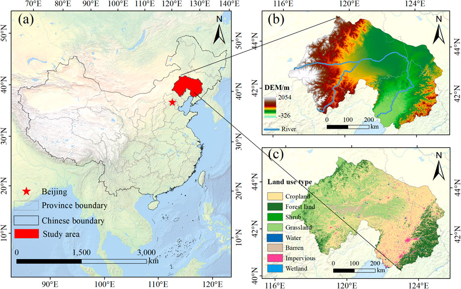
Figure 1. Location (a), DEM (b) and Land use type (c) of the Liaohe River Basin.

2.2 Data sources and processing

This research data mainly involved land use data, digital elevation model data, meteorological data, soil data, remote sensing imagery, and socioeconomic data. An overview of the data sources and preprocessing methods is provided in Table 1. All datasets were resampled to a uniform spatial resolution of 250 m and projected to the WGS 1984 UTM Zone 51N coordinate system. Image preprocessing and spatial analyses were conducted using ArcGIS 10.8.

Table 1

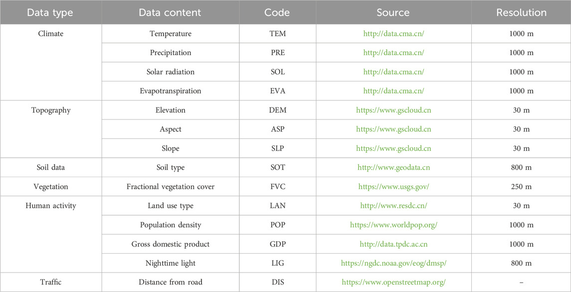
Table 1. Research data used in this study.

2.3 Data analysis

The technical framework of this study (Figure 2) consists of three main components: ecological source identification, ecological corridor construction, and multi-scenario simulation. First, We calculated TES by integrating five key ESs: CS, HQ, FP, SC, and WY. SOM were employed to classify ES bundles, and ecological sources were extracted using MSPA. Second, the drivers of TES were analyzed using the Geodetector model to identify dominant influencing factors and assign weights based on classified value intervals. These factors, combined with the spatial distribution of HQ, were used to construct a resistance surface. Based on this resistance surface, ecological corridors were identified using the MCR model, thereby forming a complete “source-corridor” ecological security pattern. Finally, three ecological security pattern scenarios (baseline, coordinated, and ideal) were coupled with four land development scenarios (business-as-usual, economic priority, coordinated development, and ecological priority). The PLUS model was used to simulate future land use changes, and the landscape pattern dynamics across different scenarios and ES bundles were compared using landscape metrics.

Figure 2

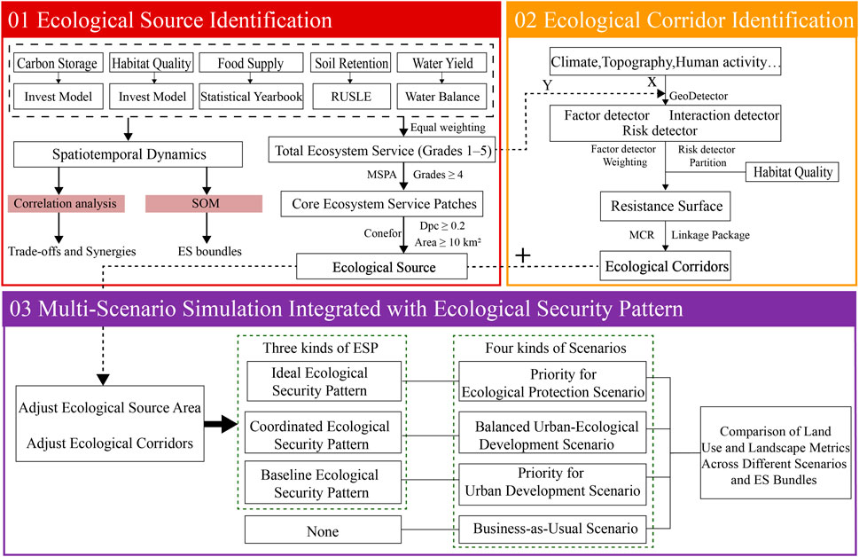
Figure 2. The research framework integrating ESP identification and land-use simulation.

2.3.1 Assessment of ESs

2.3.1.1 Carbon storage

Carbon storage represents the accumulation of organic carbon through plant photosynthesis and ecosystem carbon cycling, which can be estimated using the InVEST Carbon Storage and Sequestration module (Peng et al., 2018). The model categorizes carbon pools into four types: aboveground biomass, belowground biomass, soil organic carbon, and dead organic matter. Total carbon storage is calculated based on land use type-specific carbon density using the following formula:

$C_{i-\text{total}}=C_{i-\text{above}}+C_{i-\text{below}}+C_{i-\text{dead}}+C_{i-\text{soil}}$

where C_i-total is the total carbon storage for land use type i (t km^-2), and C_i-above, C_i-below, C_i-dead, C_i-soil represent carbon in the respective pools (t km^-2). C_i-above represents carbon stored in plant parts such as trunks, branches, leaves, and stems; C_i-below indicates carbon in the root systems; C_i-dead and C_i-soil represent the carbon densities of dead organic matter and soil organic carbon respectively.

2.3.1.2 Food supply

Food supply reflects the provisioning ES of biomass-based production, and serves as an indicator of agricultural and ecological productivity across landscapes. In this study, it was estimated using provincial statistical yearbooks combined with the spatial distribution of NDVI. The total agricultural, forestry, animal husbandry, and fishery output values were spatially allocated to cropland, forest, grassland, and water bodies based on land use type (Yang K. et al., 2024). The calculation formula is as follows:

$F{S}_i=\frac{\left(NDV{I}_i-NDV{I}_{i-\mathit{min}}\right)}{\left(NDV{I}_{i-\mathit{max}}-NDV{I}_{i-\mathit{min}}\right)}\times G_i$

where FS_i is the food supply value for pixel i, expressed in million CNY·km^-2·a⁻¹, and G_i is the gross output value for land use type i (million CNY·km^-2·a⁻¹). NDVI_i denotes the Normalized Difference Vegetation Index at pixel i, and NDVI_i-min and NDVI_i-max represent the minimum and maximum NDVI values for pixel i, respectively.

2.3.1.3 Habitat quality

Habitat quality is closely associated with regional biodiversity and ecological integrity, which can be quantified using the InVEST Habitat Quality module (Li et al., 2025). This module assumes that biodiversity is higher in areas with better habitat quality, which is evaluated based on habitat suitability and the intensity of anthropogenic threats. The formula is as follows:

$Q_{xj}=H_j\times \left[1-\left(\frac{D_{xj}^z}{D_{xj}^z+k^z}\right)\right]$

where Q_xj is the habitat quality of raster cell x for land use type j, a unitless index ranging from 0 (lowest quality) to 1 (highest quality); H_j is the habitat suitability, a dimensionless value indicating the ability of that land type to support biodiversity; D^z_xj is the threat level, and k is a half-saturation constant.

2.3.1.4 Soil retention

Soil retention represents a key regulating ES that helps prevent land degradation, sustain soil fertility, and reduce sediment transport into water bodies. It can be evaluated using the Revised Universal Soil Loss Equation (RUSLE) (Cao et al., 2020; Ma, 2020), which estimates the difference between potential and actual soil erosion. The formula is as follows:

$A=R\times K\times LS\times \left(1-C\times P\right)$

where A is the soil retention (t∙ha^-1∙a⁻¹), quantifies the ecosystem’s capacity to reduce soil erosion and maintain land productivity. R is rainfall erosivity (MJ∙mm∙ha^-1∙h^-1∙a⁻¹); K is soil erodibility (t∙ha∙h∙ha^-1∙MJ^-1∙mm^-1); LS is the slope length-gradient factor, C is the cover-management factor, representing the influence of vegetation and land cover; P is the support practice factor.

2.3.1.5 Water yield

Water yield represents a critical regulating ES that supports freshwater supply, ecosystem productivity, and hydrological balance. Evaluating its spatial distribution helps to identify water conservation zones and inform integrated watershed management. Water yield is assessed using a water balance approach based on grid cells. The yield for each cell is calculated as the difference between precipitation and evapotranspiration. The formula is expressed as follows:

$Y_{xj}=\left(1-\frac{AE{T}_{xj}}{P_x}\right)\times P_x$

where Y_xj is the water yield of raster cell x with land use type j (mm), P_x is the annual average precipitation, and AET_xj is the actual evapotranspiration (mm), which includes water losses through both plant transpiration and soil evaporation. P_x indicates the total water input in the system and AET_xj reflects the ecosystem’s water consumption based on land cover, soil properties, and climatic conditions.

2.3.1.6 Total Ecosystem Service index (TES)

TES serves as a comprehensive indicator that integrates multiple ecosystem functions into a single metric, enabling holistic assessments of regional ecological performance and spatial prioritization for ecological planning. In this study, given the differences in measurement units across ESs, each service indicator was normalized to a [0,1] scale. Then, the normalized values were aggregated and renormalized to obtain the TES (Xue et al., 2023; Bai et al., 2025). The formula is as follows:

$\begin{array}{l}E{S}_{iSTD}=\frac{E{S}_i-E{S}_{i-\mathit{min}}}{E{S}_{i-\mathit{max}}-E{S}_{i-\mathit{min}}}\\ TES={\displaystyle \sum _{i=1}^n}E{S}_{iSTD}\end{array}$

where ES_iSTD is the standardized value of ES i, and TES is the final Total Ecosystem Service index.

2.3.2 Trade-offs and synergies of ecosystem services

Correlation analysis is a statistical method used to assess the strength and direction of the relationship between two variables. Pearson’s correlation coefficient is widely applied to evaluate the linear association between continuous variables and does not impose strict distributional assumptions (Wang S. et al., 2024). In this study, Pearson’s correlation was employed to examine the synergistic and trade-off relationships among the five ES and the TES. The formula is expressed as follows:

${\rho }_{X,Y}=\frac{cov\left(X,Y\right)}{{\sigma }_X{\sigma }_Y}=\frac{E\left(X-{\mu }_X\right)E\left(Y-{\mu }_Y\right)}{{\sigma }_X{\sigma }_Y}$

where ρ_X,Y denotes the Pearson correlation coefficient between variables X and Y, cov(X,Y) is the covariance of the two variables, and σ_X and σ_Y are the standard deviations of X and Y, respectively.

2.3.3 Identification of ES bundles

In this study, SOM was employed to cluster the standardized ES data. SOM is an unsupervised learning method that projects high-dimensional data onto a lower-dimensional space while preserving the topological structure, making it well-suited for identifying underlying patterns of service combinations (Dou et al., 2020; Hu et al., 2025). The SOM network was trained using the “Kohonen” package in R (version 4.4.2), with five standardized ES indicators as input variables. The optimal grid size was determined based on quantization and topographic errors. Hierarchical clustering was then applied to group the SOM output into distinct ES bundles, providing a foundational classification for subsequent ecological security pattern construction and scenario-based simulations.

2.3.4 Geodetector for spatial differentiation and driver analysis

Spatial heterogeneity is a fundamental characteristic of geographic phenomena. The Optimal Parameters Geographical Detectors (OPGD), proposed by Song et al. (Song et al., 2020), is a suite of statistical tools designed to detect spatial variation and identify its underlying driving factors. The OPGD automatically determines the optimal discretization method and number of strata for each continuous variable by maximizing the q-statistic, thus eliminating the need for manual stratification. This study employed three core modules of Geodetector: the Factor Detector, Interaction Detector, and Risk Detector.

The Factor Detector quantified the explanatory power of natural and anthropogenic factors on the spatial differentiation of the TES (Zheng et al., 2021). The q-statistic is defined as:

$q=1-\frac{{\sum }_{h=1}^L{N}_h{\sigma }_h^2}{N{\sigma }^2}$

where L is the number of strata for the factor, N_h and N denote the number of units in stratum h and the entire region, respectively, and σ²_h and σ² are the variances of TES in stratum h and the whole region. The q-value ranges from 0 to 1, with higher values indicating stronger explanatory power.

The Interaction Detector was used to assess whether the combined effect of two factors on TES was enhanced, weakened, or independent. The Risk Detector identified whether significant differences would exist in the mean TES across different strata of a given factor (Xu et al., 2022), revealing spatial thresholds and critical zones for targeted ecosystem management.

The selection of potential influencing factors was based on ecological relevance, spatial applicability, data availability, and references from previous studies. Eleven variables were ultimately retained and categorized into five groups: climate (temperature, precipitation, solar radiation), topography (elevation, slope), soil type, fractional vegetation cover, and human activity (land use type, population density, gross domestic product, nighttime light). Variables such as aspect and road density were excluded due to low explanatory power or multicollinearity. To ensure there was no significant multicollinearity among the selected variables, we conducted a Variance Inflation Factor (VIF) analysis, and the results confirmed acceptable collinearity levels (Supplementary Table S1).

2.3.5 Construction of the ecological security pattern

Ecological sources serve as the core areas for maintaining landscape connectivity, conserving biodiversity, and sustaining ecological processes. They play a crucial role in supporting ES provision, enhancing regional ecological resilience, and ensuring functional continuity across landscapes (Fu et al., 2020). MSPA, a mathematical morphology-based image processing technique, enables the precise delineation of landscape element boundaries and types, thereby revealing spatial pattern characteristics and ecological connectivity (Nie et al., 2023). In this study, the TES index was first classified into five levels across the entire LRB. Levels 4 and 5 were defined as ecological “foregrounds” to represent areas of high ecological potential. Using the Guidos Toolbox 3.0 software (Vogt and Riitters, 2017), MSPA was performed to extract core patches. Subsequently, ecological sources were identified by applying a minimum patch size threshold and a landscape connectivity index (dPC) to filter the core areas with high ecological significance (Figure 3).

Figure 3

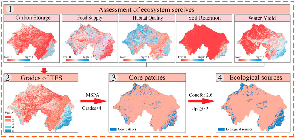
Figure 3. Workflow for the identification of ecological sources.

Ecological corridors are essential linkages within ecological networks, facilitating species migration, energy flow, and contributing to the mitigation of habitat fragmentation, enhancement of landscape connectivity, and continuity of ecological processes (Huang et al., 2021). To quantify ecological resistance between core areas, this study innovatively integrated both natural and anthropogenic driving factors using the results of the geographical detector. Specifically, dominant factors with an explanatory power (q value) greater than 0.1 were selected through the Factor Detector module. Subsequently, sub-intervals of each driving factor were scored based on the Risk Detector results, where lower TES values were assigned higher resistance scores. The resistance surface was calculated using a weighted sum of all selected driving factors, incorporating both their explanatory power and spatial value distribution:

$\begin{array}{c}{w}_k=\frac{q_k}{Q}\\ S_i={\displaystyle \sum _{k=1}^m}{w}_k\times c_k\end{array}$

where S_i is the resistance value for pixel i, w_k is the weight of the factor k, equal to its q value divided by the total q value of all selected factors, and c_k is the assigned resistance score of the factor k for pixel i.

Areas with higher habitat quality correspond to lower ecological resistance, as they offer greater ecological suitability and species persistence (Lin et al., 2016). To account for habitat integrity and landscape ecological function, the inverse of the Habitat Quality (1 – HQ) was integrated as a key component in constructing the ecological resistance surface. This approach reflects an ecological rationale that intact habitats facilitate ecological flows, while degraded or fragmented areas pose greater resistance (Zhang et al., 2025). Accordingly, we assigned equal weights (0.5 each) to the standardized resistance layer derived from anthropogenic and biophysical drivers, and the inverse HQ layer, and then overlaid them to produce the final ecological resistance surface for the LRB (Wang et al., 2022).

To delineate ecological corridors, we adopted an integrated approach combining the MCR model and circuit theory. This approach enables the consideration of both landscape resistance gradients (captured by MCR) and probabilistic ecological flow pathways (captured by Linkage Mapper), thereby enhancing the spatial realism and robustness of corridor identification in heterogeneous landscapes, particularly in heterogeneous landscapes with complex barrier effects (Fan et al., 2022; Zhang et al., 2024). Based on the constructed resistance surface, ecological corridors were extracted using the Linkage Mapper tool (version 3.0.0) by setting appropriate parameters for corridor width and maximum linkage distance. These corridors were subsequently overlaid with the identified ecological source areas to construct the complete ecological security pattern across the basin (Figure 4).

Figure 4

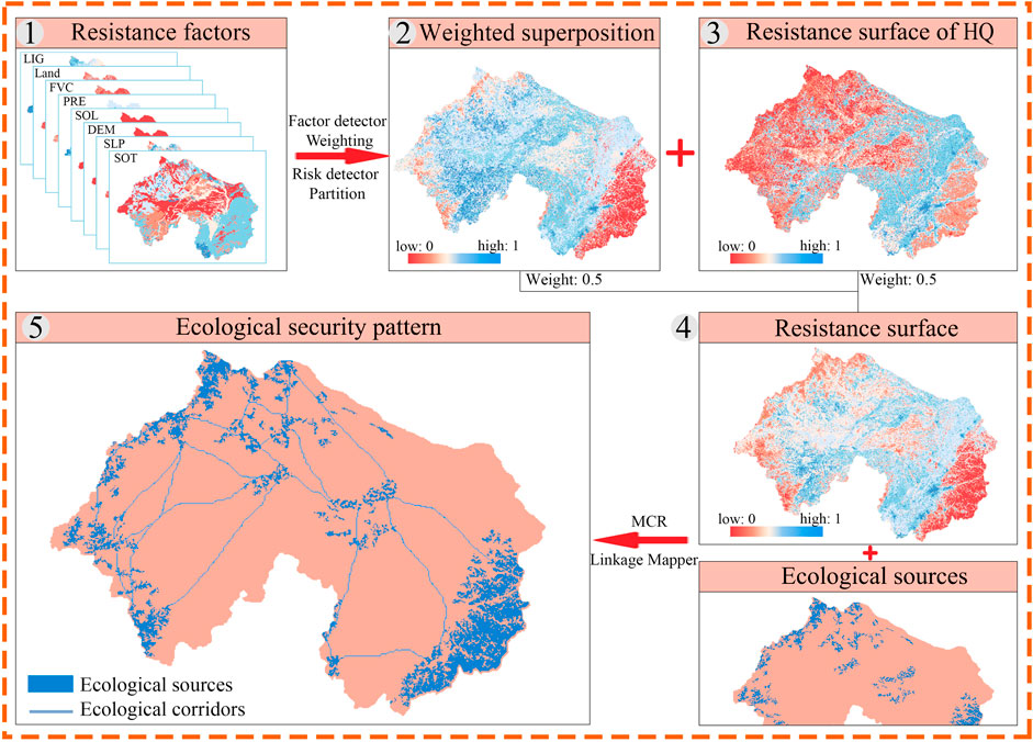
Figure 4. Ecological security pattern construction.

To accommodate varying protection levels and land management strategies, this study, drawing upon previous research (Wang et al., 2021), established three ecological security pattern (ESP) schemes: (1) Baseline Ecological Security Pattern (BESP): minimum core patch area ≥100 km², dPC ≥0.2, corridor width = 1 km; (2) Coordinated Ecological Security Pattern (CESP): minimum core patch area ≥50 km², dPC ≥0.2, corridor width = 1.5 km; (3) Ideal Ecological Security Pattern (IESP): minimum core patch area ≥20 km², dPC ≥0.2, corridor width = 2 km. These three schemes reflect a gradient of ecological protection intensities and provide a hierarchical scientific basis for ecological redline delineation and spatial restoration planning.

2.3.6 PLUS model and four regional development scenarios

The Patch-generating Land Use Simulation (PLUS) model is a land use change simulation framework that integrates cellular automata, random forest algorithms, and multi-factor drivers. It is capable of simulating the spatial expansion of land use patches with high accuracy based on raster datasets (Liang et al., 2021). The model consists of two core modules: the Land Expansion Analysis Strategy (LEAS), which extracts land expansion patterns, and the Cellular Automata based on Multiple Random Seeds (CARS), which employs a random forest algorithm to evaluate the contributions of driving factors and simulate patch-level growth. Combined with Markov chains, the PLUS model enables spatial prediction of land use under multiple scenario settings (Wang and Liu, 2025).

In this study, four future development scenarios were defined for the LRB: Business-as-Usual (BAU), Economic Priority (PUD), Coordinated Development (BUE), and Ecological Priority (PEP). Each scenario was integrated with corresponding ESP constraints to enhance the ecological rationality and policy relevance of the simulations. Land demand was projected using the Markov chain module of the PLUS model, based on historical land use transitions from 2000 to 2020. In addition, scenario-specific goals were achieved by adjusting the transition probabilities between different land use types, such as increasing the conversion rate from ecological land to construction land in PUD, or limiting urban expansion and enhancing ecological restoration in PEP. Detailed parameter settings are provided in Table 2.

Table 2

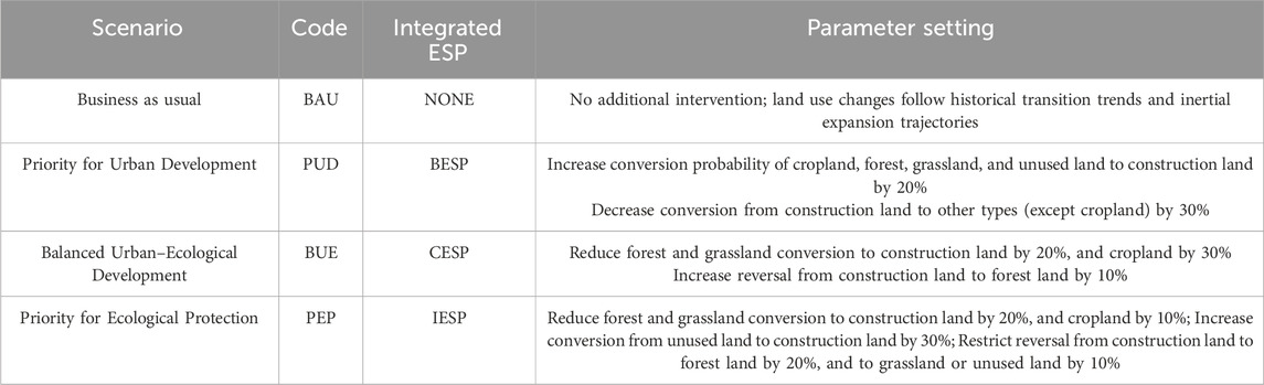
Table 2. Description of four regional development scenarios, corresponding ESP constraints, and transition probability adjustment rules.

According to previous studies, a Kappa coefficient greater than 0.7 is generally indicative of high simulation accuracy [24]. In this study, we used 2010 land use data to simulate the land use pattern of 2020, yielding a Kappa coefficient of 0.71 and an overall accuracy of 78%, demonstrating that the PLUS model has a good fit and strong predictive capability. Based on these results, we used 2020 land use data as the base year and incorporated different land expansion probabilities under the four defined development scenarios to simulate the land use patterns for 2030. Additional model parameters are listed in Supplementary Table S2.

2.3.7 Scenario comparison using landscape metrics

Landscape pattern metrics are essential tools for quantifying the spatial structure of land use and have been widely applied in landscape ecological analysis and ecological effect evaluation (Boongaling et al., 2018). Following previous studies (Jiao et al., 2019), six representative metrics were selected in this study: the Number of Patches (NP) and the Landscape Division Index (DIVISION) were used to characterize the degree of landscape fragmentation; the Shannon Diversity Index (SHDI) and Shannon Evenness Index (SHEI) were adopted to assess the richness and evenness of landscape types; the Cohesion Index (COHESION) and the Contagion Index (CONTAG) were applied to describe the spatial aggregation and dispersion patterns of landscape patches. All metrics were calculated using the Fragstats 4.2 software, enabling a comprehensive assessment of spatial heterogeneity and changes in ecological connectivity across different land use scenarios.

3 Results

3.1 Ecological source identification

3.1.1 Spatial distribution and variations of ecosystem services

According to Figure 5 and Supplementary Table S3, ESs in the LRB exhibited varying trends from 2000 to 2020. CS showed a steady increase, with the average rising from 7.54 t/ha to 7.89 t/ha, and the total amount growing from 1.85 × 10⁹ t to 1.94 × 10⁹ t. Spatially, the eastern and western margins maintained higher values than the central region, with a more pronounced increase in the east. FS experienced a significant boost, with unit output rising from 0.22 to 1.10 million CNY/km². The gross output of agriculture, forestry, animal husbandry, and fishery increased by 193.82 billion CNY over the 2 decades, especially in regions with dense cropland. HQ declined slightly from 0.49 to 0.47, particularly in areas with new roads and urban expansion, indicating the negative impact of urbanization on ecological integrity. SR and WY both showed fluctuating upward trends, with average increases of 12.94 t/hm² and 44.23 mm, respectively. Their total amount increased by 45 million tons and 10 billion m³, respectively, both reaching their lowest levels in 2015. Spatially, soil retention was higher in the eastern and western fringes, while water yield decreased from east to west, with significant increases in the west and declines in the northeast. The TES remained relatively stable, increasing slightly from 0.33 to 0.35, with an average annual value of 0.33. TES exhibited a typical “high in the east and west, low in the center” spatial pattern, with a slightly increasing trend over time, and a larger area showing increases than declines.

Figure 5

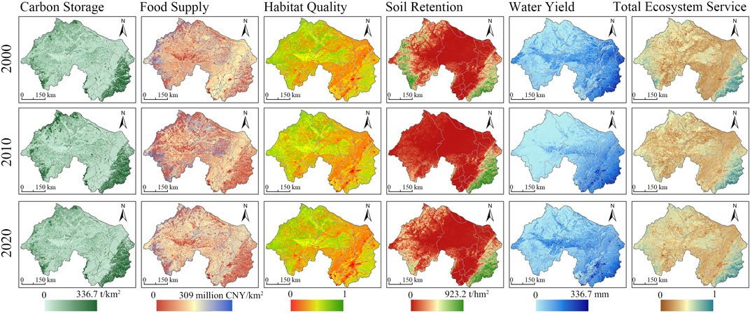
Figure 5. Spatial-temporal dynamics of five Ess and TES (2000–2020).

3.1.2 Trade-offs and synergies of ESs

According to the multi-year average analysis (Figure 6), TES exhibited a positive synergy with all individual ESs. The highest correlation was observed with CS (r = 0.67), while the lowest was with WY (r = 0.10), indicating that TES effectively captures the overall spatial patterns of multiple ecosystem functions. Notably, WY showed trade-off relationships with HQ, FP, and CS, suggesting spatial mismatches between water-related services and other ecological functions. This also explains the relatively weak correlation between WY and TES. Meanwhile, moderate trade-offs were observed between FP and both SR and CS, likely due to the spatial and resource demands of agricultural production. Overall, aside from these trade-offs, the remaining ES pairs showed strong synergies and high spatial consistency. For example, the interannual correlation coefficients between WY and SR from 2000 to 2020 were 0.09, 0.34, 0.43, 0.06, and 0.18, respectively. Although fluctuations existed, the correlation remained positive, with an average annual coefficient of 0.23, indicating a weak but persistent synergy between the two services.

Figure 6

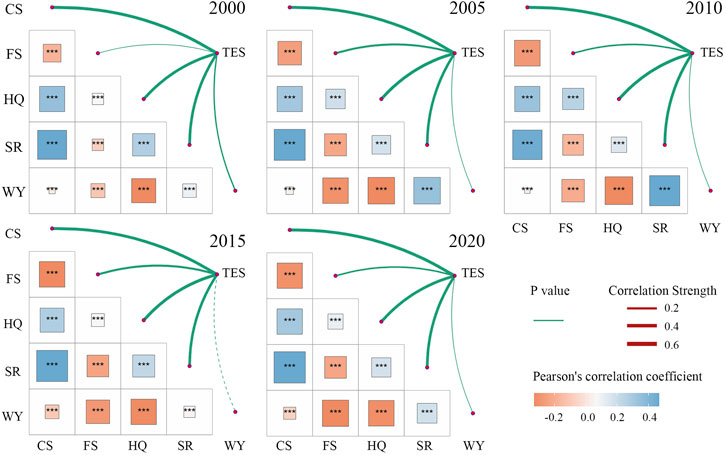
Figure 6. Trade-offs and synergies Between ESs (2000–2020).

3.1.3 Spatial bundles for ESs

Based on the spatial distribution and pairwise trade-off–synergy relationships of ESs, the SOM method was applied to classify the LRB into six distinct ES bundles (Figure 7). These were designated as follows: Comprehensive Service Function Bundle (CSFB), Agricultural Development Priority Bundle (ADPB), Eco-Agricultural Synergy Bundle (EASB), Water Conservation Priority Bundle (WCPB), Ecological Transition Buffer Bundle (ETBB), and Ecological Protection Buffer Bundle (EPBB).

Figure 7

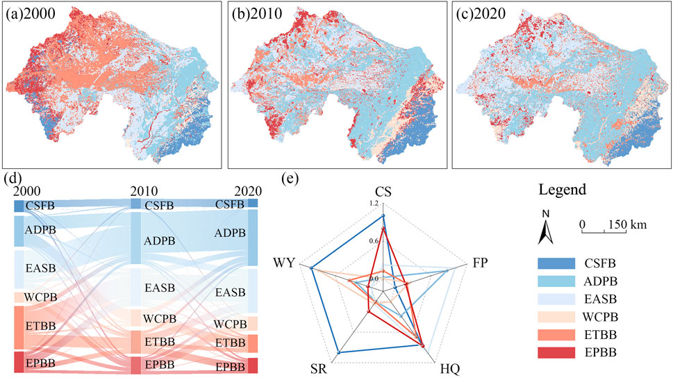
Figure 7. Temporal dynamics and functional traits of six ES bundles: (a–c) Spatial distribution of bundles in 2000, 2010, and 2020; (d) Transitions among bundles from 2000 to 2020; (e) Functional profiles based on five ES indicators.

The CSFB demonstrated the most comprehensive ecosystem performance, with the highest values for CS, WY, SR, and HQ, resulting in the highest TES (0.55). This area was recognized as the core ecological high-energy zone of the basin (Supplementary Table S4). The ADPB was dominated by FP (0.80) but exhibited weak ecological functions, with a composite index of only 0.27, indicating a need for enhanced ecological degradation control. The EASB combined the highest FP (0.88) with the best HQ (0.62), making it suitable for the development of eco-agriculture and ideal for future “green granary” planning. The WCPB was characterized by high WY (263.34 mm) but showed relatively weak ecological foundations, marking it as a key zone for water resource protection. The ETBB displayed moderate values across all services, with a TES of 0.30, functioning as a buffer zone between multifunctional areas. The EPBB had relatively high CS (17.01 t/ha) and HQ (0.57), while FP and WY were limited, underscoring its role as a stable ecological buffer adjacent to core ecological source areas. From 2000 to 2020, the spatial distribution of service bundles underwent significant changes. Notably, the proportion of the ADPB increased from 16.6% to 35.8%, an increase of 19.2%, while the ETBB declined from 27.6% to 11.4%, a reduction of 16.2%, reflecting a marked trend of agricultural expansion and contraction of transitional ecological zones.

At the grid scale, the CSFB was primarily distributed in the eastern forested areas, characterized by a combined advantage in CS, HQ, and WY. The ADPB was concentrated in the northern and western plains, where FP dominated and ecological functionality was limited. The remaining four bundles were spatially located in the northwest, southeast, central, and peripheral areas of the basin, reflecting transitional and composite characteristics of ESs. At the county scale, many counties in the northwest were dominated by agricultural functions, while counties in the southwest emphasized comprehensive service provision and ecological protection, forming critical ecological barriers. The EASB and ETBB were sporadically distributed across the central hilly areas and southeastern edges. At the city scale, dominant service types became more simplified: the central region was primarily oriented toward agricultural production, whereas southeastern cities were characterized by integrated ecological service provision (Figure 8). Although spatial detail was reduced at the municipal level, this scale offered stronger policy relevance and can better support ecological redline delineation and territorial spatial planning.

Figure 8

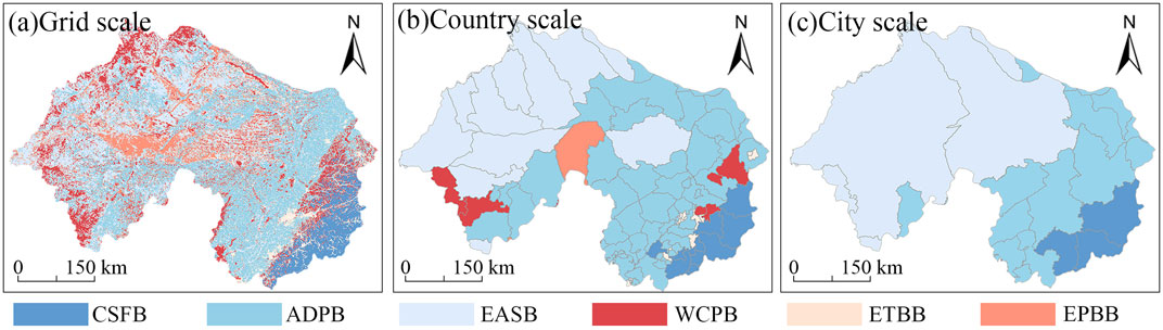
Figure 8. Spatial distribution of ecosystem service bundles at grid (a), county (b), and city scales (c).

3.1.4 Spatial distribution and variations of core patches

From 2000 to 2020, the spatial distribution of core ecological patches in the LRB remained generally stable, primarily concentrated in the southeastern mountainous and hilly regions (e.g., Yiwulü Mountains, Qianshan Mountains, and the upper reaches of the Hun River), where vegetation cover was dense and human disturbance was relatively low (Figure 9). Although the spatial pattern did not shift significantly, the total area of core patches exhibited a decline–recovery trajectory over the 2 decades: decreasing from 20,651 km² in 2000 to 14,773 km² in 2010, then rising to 22,623 km² in 2020—resulting in a net gain of 1,972 km². This trend reflected early-stage disturbances caused by urban expansion and land use changes, followed by ecosystem restoration outcomes associated with ecological projects implemented after 2010.

Figure 9

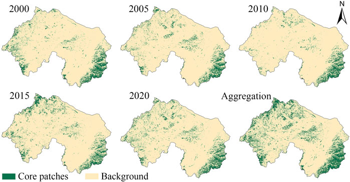
Figure 9. Spatial-temporal dynamics of core patches (2000–2020).

3.2 Ecological corridors construction

3.2.1 Driver analysis of TES

According to the single-factor detection results from the Geodetector model (Figure 10), LAN consistently emerged as the dominant driver of the spatial heterogeneity of the TES across all years, with an average q-value of 0.538. This was followed by FVC, PRE, and SOL, with q-values of 0.244, 0.231, and 0.138, respectively, indicating that both natural environmental conditions and vegetation status played vital roles in shaping TES patterns. The explanatory power of LAN remained relatively stable from 2000 to 2020 (q = 0.488–0.584). In contrast, anthropogenic factors such as LIG showed an increasing trend in recent years, reflecting the growing impact of urban expansion on the spatial configuration of ESs. Overall, TES spatial heterogeneity was jointly shaped by LAN and natural factors, while the influence of human activities intensified over time, underscoring the need to incorporate ecological safeguards into land-use optimization and urban growth strategies.

Figure 10

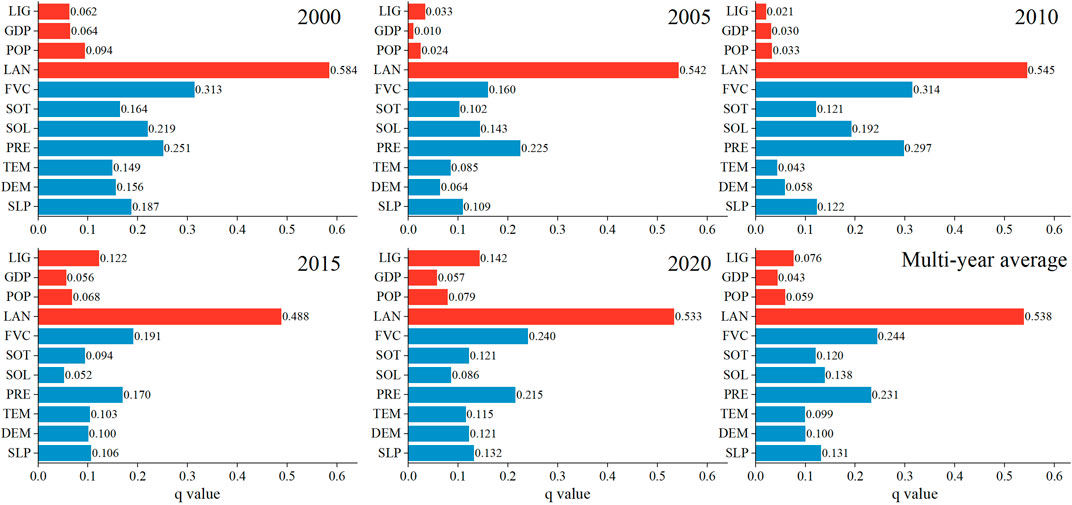
Figure 10. Results of single factor detection across the entire LRB (2000–2020). Note: LIG (Nighttime Light); GDP (Gross domestic product); POP (Population density); LAN (Land use type); FVC (Fractional vegetation cover); SOT (Soil type); SOL (Solar radiation); PRE (Precipitation); TEM (Temperature); DEM (Elevation); SLP (Slope).

At the bundle level (Figure 11), the CSFB was primarily driven by FVC (q = 0.491), along with DEM (q = 0.244) and PRE (q = 0.193), highlighting the critical role of natural environmental conditions in supporting ecosystem functionality. The ADPB was dominantly influenced by LAN (q = 0.226), and its overall low q-values suggested limited ecological function diversity and high sensitivity to human exploitation. The EASB was chiefly regulated by LAN (q = 0.413), while also affected by soil and vegetation factors, reflecting its dual attributes of production and ecology. The WCPB was jointly shaped by PRE (q = 0.321) and LAN (q = 0.364), underscoring the importance of hydrological processes. Both the ETBB and EPBB were influenced by multiple co-acting factors. Overall, the heterogeneity of dominant drivers across bundles confirmed the complex mechanism underlying spatial ES patterns, driven by the combined effects of natural gradients and land use dynamics.

Figure 11

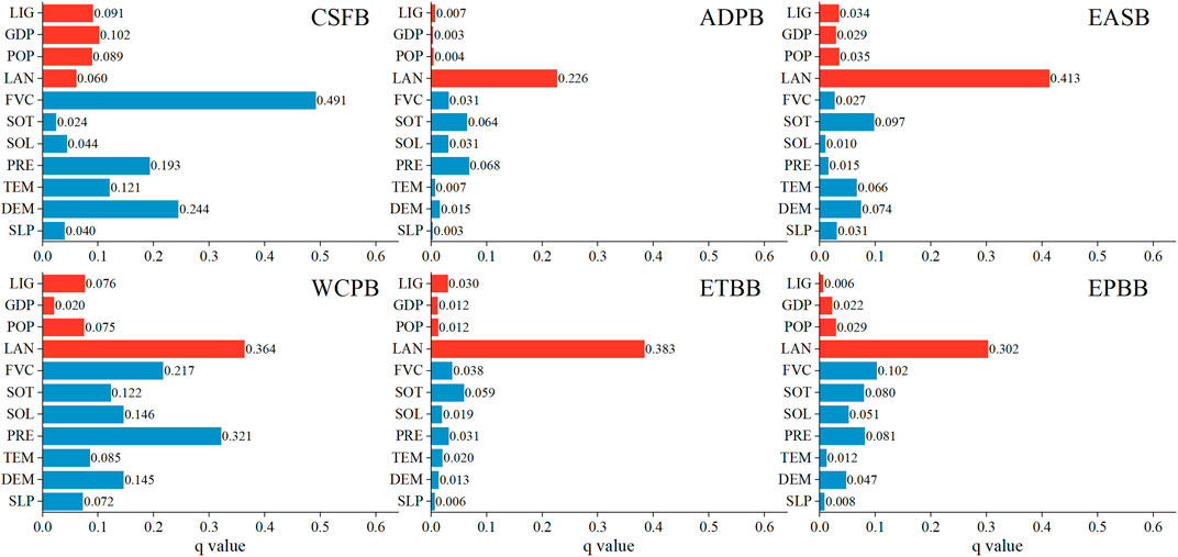
Figure 11. Results of single factor detection across ES bundles in 2020.

The driving mechanisms of ESs exhibited a pronounced “dual-factor enhancement effect” (Figure 12). According to the multi-year average analysis, the strongest interaction was observed between LAN and FVC, with a q-value of 0.64. This was followed by interactions between LAN and SLP (q = 0.59), FVC and SLP (q = 0.57), and FVC and (POP (q = 0.56). All of these combinations exceeded a q-value of 0.55, indicating significant coupling between land use, topography, and vegetation structure, which collectively played a critical role in shaping the spatial distribution of eESs. Notably, interactions between socio-economic factors—such as POP and FVC, and GDP and LAN—also exhibited moderately high q-values across all years, suggesting that the interplay between human activities and vegetation status had a sustained impact on ES patterns.

Figure 12

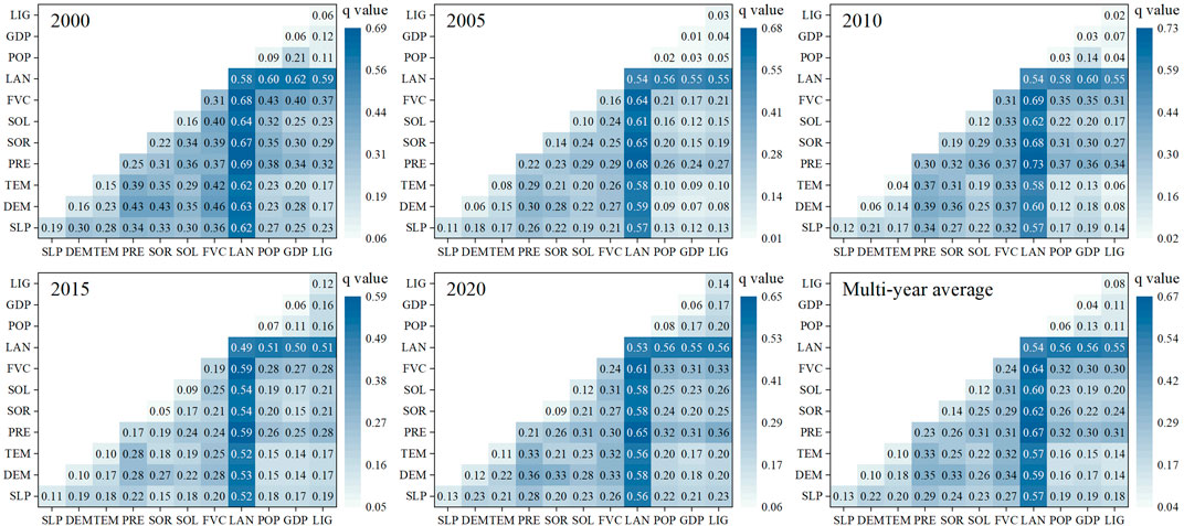
Figure 12. Interaction detection of driving factors across the entire LRB (2000–2020).

The Risk Detector module was applied to identify the sensitive intervals of key drivers affecting ESs (Figure 13). The more detailed classification method can be seen in Supplementary Figure S1. The results indicated that the TES was positively correlated with DEM, SLP, PRE, and FVC, while it was negatively correlated with TEM, POP, GDP, and LIG. High TES values were typically found in regions with favorable natural conditions and low human disturbance, primarily located in the mountainous and hilly areas of southern and southeastern LRB. These areas were characterized by higher DEM, greater PRE, lower TEM, moderate SOL, and steeper SLP. Highly active Luvisols and dense vegetation coverage strongly supported ES performance, with forest land being the most favorable land use type for ES provision (Supplementary Table S5). Moreover, areas with lower values of POP, GDP, and LIG consistently exhibited higher TES levels, emphasizing that low-intensity human disturbance was a key factor in maintaining high ES capacity.

Figure 13

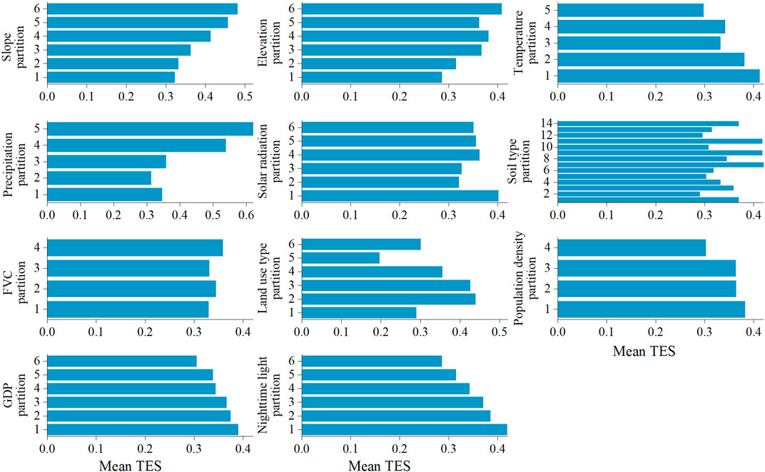
Figure 13. Risk detection of driving factors based on subsection analysis across the entire LRB. Note: A larger partition value indicates a higher corresponding driver value, except for LAN and SOT, which are categorical variables and do not represent continuous gradients.

3.2.2 Resistance surface construction

The weights and assigned values of each driving factor used in constructing the resistance surface are summarized in Supplementary Table S6. The ecological resistance across the LRB exhibited pronounced spatial heterogeneity (Figure 14). Low resistance values were generally found in the southeastern hilly areas and forested regions, indicating better ecological connectivity. In contrast, higher resistance values dominated the southwestern parts, central urban expansion zones, and agropastoral ecotones, where ecological processes were more severely disturbed. The average resistance map across the three time periods showed a relatively stable spatial pattern; however, certain areas—particularly in the central and western regions—exhibited increasing resistance trends, suggesting persistent anthropogenic pressure on ecological connectivity.

Figure 14

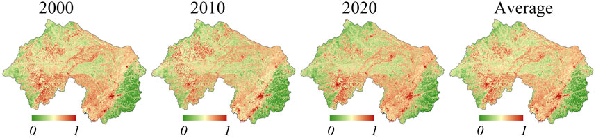
Figure 14. Spatial distribution of resistance surface (2000–2020). Note: From green to red indicates increasing resistance values, with red representing the highest resistance.

3.3 Multi-scenario simulation integrated with ESP

3.3.1 Three types of ecological security patterns

The cumulative core patch layer (Figure 9), derived from multi-year aggregation analysis, was used for landscape connectivity assessment. Patches with dPC ≥0.2 were identified, and three types of ecological source areas were delineated by adjusting the minimum patch area threshold. The multi-year averaged ecological resistance surface (Figure 14) was then used to extract ecological corridors based on the MCR model, with varying corridor widths corresponding to three scenarios. By integrating source patches and ecological corridors, three hierarchical ESPs were constructed: the BESP, CESP, and IESP. As the spatial constraints were gradually relaxed, the extent of both ecological sources and corridors significantly expanded, leading to enhanced connectivity and a more integrated ecological network structure (Figure 15).

Figure 15

Figure 15. Spatial distribution of three types of ESPs.

In the BESP, ecological sources were mainly concentrated in the northwestern mountainous zones and the southeastern forest-grassland transition zones of the LRB, with a total area of 30,740.88 km². The corridors were sparsely distributed, covering only 7,994.18 km², resulting in a fragmented, locally connected network that provided limited support for ecological processes. Under the CESP, the source area increased to 39,506.50 km², with new sources expanding into the central agro-forestry ecotone and the southern hilly transition zone. The total length of corridors reached 13,469.70 km², forming a spatial network characterized by a north-south backbone and east-west branches, which substantially improved connectivity and ES provision. In the IESP, ecological sources further expanded to 47,631.06 km²—approximately 1.55 times that of the BESP. The newly added sources were widely distributed in the central and southeastern ecologically sensitive zones. Corridor coverage reached 20,839.85 km², forming a dense, multi-pathway corridor network that significantly enhanced connectivity and system stability. This configuration established a complete “source–corridor” structure capable of supporting multi-scale species migration, energy flow, and ecological process continuity.

Overall, the three ESPs demonstrated a clear hierarchical progression. Both the CESP and IESP exhibited superior performance in maintaining ecological integrity and enhancing spatial permeability, offering differentiated spatial planning guidance for land-use regulation and ecosystem restoration strategies.

3.3.2 Land use changes and transition patterns under different scenarios

Figure 16 illustrates the spatial patterns, structural changes, and transition pathways of land use in the LRB for the baseline year of 2020 and under four development scenarios (BAU, PUD, BUE, and PEP), each coupled with corresponding ecological security patterns. Spatially, cropland remained relatively stable across all scenarios and was predominantly distributed in the central and northern plains. In the PUD scenario, construction land expanded most significantly, encroaching on large areas of cropland and forest. In contrast, the PEP scenario effectively constrained the expansion of construction land, preserving forest and grassland areas, which highlights the regulatory impact of ecological conservation policies. In terms of land composition, grassland areas increased under all scenarios, reaching a maximum of 68,894 km² in the PEP scenario. Forest area showed the sharpest decline in the PUD scenario, while remaining stable in the PEP scenario. Construction land expanded significantly under PUD (up to 12,079 km²), substantially higher than under PEP (10,865 km²). Cropland-to-construction transitions represented the dominant land use change across scenarios, particularly in the PUD scenario. Conversions from forest to grassland were also common, indicating ongoing ecological restoration and reforestation efforts. However, the forest-to-construction transitions were significantly reduced in the PEP scenario, reflecting strong suppression of development under ecological priorities.

Figure 16

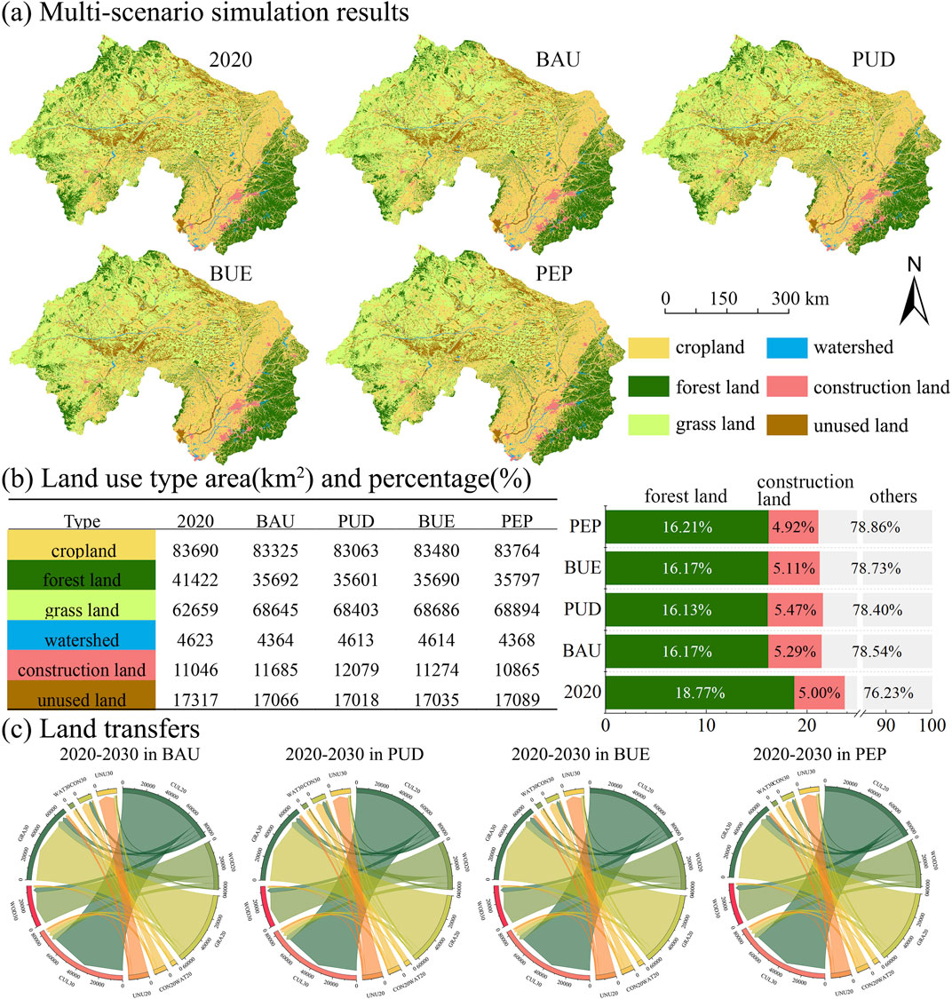
Figure 16. Land use simulation and transition under multiple development scenarios for 2030: (a) Multi-scenario simulation results; (b) Land use type area (km²) and percentage (%); (c) Land transfers.

Specifically, forest area decreased by only 645 km² under PEP, compared to 1,751 km² under PUD—a reduction of 63.2%. This substantial difference underscored the effectiveness of eco-prioritized spatial regulation, particularly in safeguarding forest areas from urban encroachment, and affirmed the protective role of “ecological red lines.” Moreover, the PEP scenario achieved a net gain in grassland area (+2,237 km²), whereas grassland increased in PUD partly resulted from forest conversion, leading to limited ecological improvement. Overall, the economically driven scenario promoted urban expansion and resource exploitation, while the ecologically oriented scenario enhanced landscape integrity and ecosystem stability—providing a scientific basis for future territorial spatial planning and restoration strategies.

3.3.3 Landscape pattern metrics responses of ES bundles under multiple scenarios

Significant differences in landscape patterns were observed among different ES bundles under the four development scenarios (Figure 17). The CSFB consistently exhibited the lowest number of patches (NP ≈ 7,700), indicating a less fragmented landscape. However, this zone also showed the lowest values in SHDI and SHEI, with the lowest SHEI reaching 0.28. This suggested a landscape structure dominated by a single land cover type—primarily forest—resulting in low heterogeneity and limited richness in landscape types. Under the PEP and BUE scenarios, slight improvements in SHDI and SHEI were observed, indicating that appropriate ecological conservation measures could help enhance landscape structure. ADPB showed the highest degree of fragmentation, with an NP of approximately 81,000, which was characteristic of intensively cultivated agricultural systems. Despite this fragmentation, the CONTAG index remained above 55 and COHESION exceeded 98.9, indicating moderate connectivity between agricultural patches. Slight increases in diversity under the PEP scenario (SHEI = 0.51) were recorded, although the overall improvement remained limited. EASB demonstrated stable connectivity and moderate diversity, with DIVISION consistently above 0.98 and COHESION above 97. SHDI and SHEI remained at medium-to-high levels, reflecting a well-integrated landscape structure between agricultural and ecological spaces. The WCPB and the ETBB exhibited the most balanced and diverse landscape structures. Notably, SHDI in ETBB exceeded 1.46 across all scenarios, and SHEI reached up to 0.83, indicating both high landscape richness and evenness. These areas also demonstrated strong ecological connectivity and regulation potential, particularly under the BUE and PEP scenarios. EPBB was characterized by high aggregation and low fragmentation, with NP ranging from 36,000 to 40,000 and SHEI consistently above 0.76, indicating a stable and coherent landscape configuration.

Figure 17

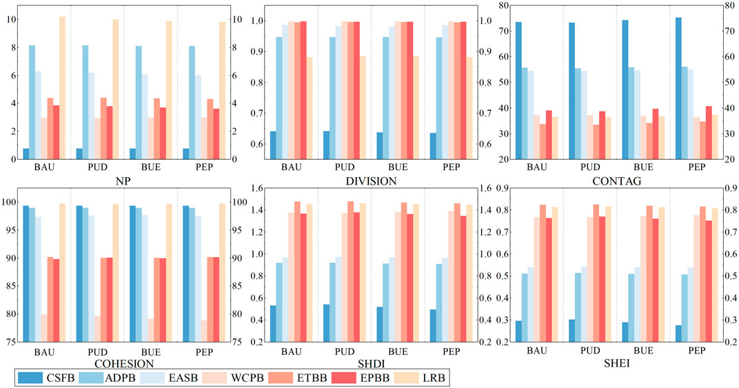
Figure 17. Comparison of landscape pattern metrics under multiple development scenarios across ES bundles.

At the basin scale, the LRB maintained relatively high landscape diversity and balance across all scenarios, with SHDI averaging around 1.45 and SHEI around 0.81. This suggested strong ecological heterogeneity and systemic integrity across the region. Notably, the PEP and BUE scenarios further enhanced the ecological structure of the basin, especially in zones dedicated to ecological buffering and water conservation, supporting the broader goal of sustainable spatial development.

4 Discussion

4.1 Spatiotemporal patterns and interactions of ecosystem services

Accurately identifying the spatiotemporal variations and interaction mechanisms of ESs is crucial for achieving efficient ecosystem management (Raudsepp-Hearne et al., 2010; Hu et al., 2025). This study revealed significant spatial heterogeneity in the ESs of the LRB. The spatial distribution of the TES was predominantly driven by land use patterns, with forested areas exhibiting the best performance across various ESs. High-value TES zones were primarily concentrated in the eastern (Changbai Mountain–Qianshan Mountain system) and western edge areas, characterized by higher elevations, extensive forest cover, and minimal human disturbance. In these areas, natural factors such as vegetation cover, precipitation, and solar radiation also played important roles in maintaining and enhancing ecosystem productivity and energy cycling (Cao et al., 2021). These ecologically valuable areas were identified as core ecological sources, serving as key nodes for species habitat and dispersal, thus providing spatial support for ES provision.

Between 2000 and 2020, the total area of core ecological patches increased by approximately 2,000 km², mainly in the northern and southeastern parts of Tongliao, where forest cover rose from 8.9% in 1978 to 19.49% in 2024, and grassland area remained stable—reflecting the substantial success of the ecological restoration projects in the LRB. In contrast, the central and eastern plains—particularly densely populated urban areas such as Shenyang and Liaoyang—feature flat terrain and intense population pressure. Rapid urbanization and intensive agricultural practices have led to ecological degradation, resulting in low-value TES areas. Temporally, human activity indicators such as nighttime light, GDP, and population have shown an increasing explanatory power for TES changes. This trend suggested that human activities, through land development and resource consumption, are continuously reshaping the supply capacity and spatial distribution of ESs.

Regarding interactions among ESs, TES exhibited a distinct spatial pattern of “synergy in the east and trade-offs in the west” with SR, WY and HQ (Supplementary Figure S2), indicating substantial regional differences in the coupling intensity of ecosystem functions. In the eastern region, favorable natural conditions and stable ecosystem structures supported strong synergistic effects among services. Conversely, in the ecologically fragile agro-pastoral transitional zones of the west, significant resource allocation conflicts were observed among water yield, soil retention, and habitat quality, resulting in pronounced trade-offs between TES and other services. Furthermore, FS and WY generally exhibited a certain degree of trade-offs with other services, consistent with the findings in the Beijing–Tianjin–Hebei urban agglomeration (Shen et al., 2020). These findings underscored the importance of prioritizing the synergy and trade-offs among ES functions in future ecosystem management, to prevent overall functional degradation resulting from the optimization of land use for a single ES (Holling and Meffe, 1996).

4.2 Dynamic shifts of ecosystem service bundles and management implications

This study incorporated the trade-offs and synergies among ESs and employed SOM approach to classify the LRB into six dominant ES bundles. The results indicated that the CSFB performed best across multiple ecological function indicators and possesses significant ecological advantages, making it a priority for designation as an ecological conservation redline area. Its superior ecological functions were primarily maintained by natural environmental factors, with key drivers including fractional vegetation cover (q = 0.491), elevation (q = 0.244), and precipitation (q = 0.193). Given their transitional functional characteristics, along with high ecological connectivity and diverse driving influences, the WCPB and EPBB are well-suited for the deployment of ecological corridors and buffering strategies. In contrast, the ADPB exhibited weak ecological functions and high landscape fragmentation, mainly driven by land use (q = 0.226). The low level of ES provision suggested heavy dependence on anthropogenic intervention, highlighting the need to strengthen farmland protection, degraded land restoration, and ecological compensation. The spatial differentiation of regional functions closely matched the supply capacity of ESs, validating the scientific and practical feasibility of using dominant ES characteristics to delineate bundles. The study recommends designating the southeastern mountainous and hilly regions (dominated by CSFB) as priority ecological protection zones, strictly limiting construction land expansion, and enhancing their disturbance resistance. Additionally, appropriate development of ecotourism industries can promote the integration of ecological education and environmental protection, raising public ecological awareness while fostering regional economic growth. In the northwestern agro-pastoral transition zone, efforts should focus on promoting ecological agriculture and grassland restoration to mitigate degradation risks and improve regional ecological functions. For urban expansion areas (such as those surrounding Shenyang and Liaoyang), the establishment of ecological buffers and multifunctional green infrastructure networks is essential to enhance ecosystem connectivity and overall service capacity.

However, these bundle-based management strategies must account for the long-term dynamic evolution of the LRB’s ecosystems. Since 2000, significant ecological engineering projects—such as the “Three-North Shelter Forest Project” and “Grain for Green Project” initiatives (Zhu et al., 2023)—have led to substantial changes in land cover within the basin. Between 2000 and 2020, 3,007.6 km² of cropland was converted to forestland and 1,591.8 km² to grassland (Supplementary Table S7), with a concurrent enhancement in regional ES levels and significant reshaping of ES bundle spatial patterns. Notably, the ETBB exhibited the most pronounced changes, with its area proportion decreasing from 27.6% to 11.4% over 2 decades, and its spatial distribution progressively contracting toward central areas. These trends indicate significant transformations in the basin’s ecosystem structure and functional zoning. Moreover, urban expansion and intensive agricultural land use have compressed natural ecological spaces, driving structural transitions among service bundles (Figure 7), consistent with findings from existing basin-scale studies (Jing and Zhiyuan, 2011). Thus, these transformations, jointly driven by major ecological projects and human activities, underscore the limitations of defining service bundle zones based solely on a single temporal snapshot, as such delineations may fail to accommodate future ecosystem dynamics (Wang et al., 2023). Future research should adopt a multi-objective optimization framework and an integrated “social–ecological–economic” perspective to comprehensively explore the dynamic drivers of bundle transitions and develop more adaptive and resilient ecosystem functional zoning systems (Lyu et al., 2024; Zhou et al., 2025).

4.3 Comparison of the ecological effectiveness of land-use transitions under different scenarios

Under the backdrop of accelerated urbanization and increasingly stringent ecological redline controls, scientifically simulating land use changes under different development pathways is of great significance. Taking the LRB as a case study, this research established a multi-scenario simulation framework integrating the ESPs and the PLUS model to evaluate future land use dynamics from the perspective of spatial restructuring, thereby providing support for high-quality and sustainable regional development. The findings indicated that under the PUD scenario, construction land expands most rapidly, resulting in a net forest loss of 4,731 km² and a reduction of 1,834 km² in cropland area. This expansion intensified landscape fragmentation (DIVISION) and decreased ecological connectivity (COHESION), reflecting an increased risk of ecological degradation under an economy-first development mode. In contrast, the PEP scenario effectively curbed unregulated expansion through the enhanced protection of ecological sources and corridors, leading to a 63.2% reduction in forest loss compared with the PUD scenario, an increase in grassland area, a 6.5% improvement in landscape aggregation, and a slight increase in the TES. These changes significantly bolstered ecosystem resilience and system connectivity. Moreover, the transition behaviors of different land-use types exerted significant impacts on ESs. For instance, the conversion of forestland to grassland was primarily concentrated in the northwestern part of the basin, resulting in reduced CS and degraded HQ. Conversely, the conversion of unused land to grassland improved overall WY and SR capacity. Notably, the scale of forestland conversion to construction land was substantially higher under the PUD scenario than in other scenarios. These results suggested that land-use changes not only reshape spatial patterns but also directly affect the provision of key ESs, underscoring the need for prioritized attention within national land-use spatial planning.

Overall, the results demonstrated that the integrated ESP–PLUS framework exhibits strong applicability and scalability for simulating land-use changes at the basin scale. By incorporating hierarchical ecological security patterns as spatial constraints and combining multi-scenario simulations with regionally differentiated management, the framework effectively mitigated ecological degradation risks associated with urbanization and enhances the supply capacity of ESs (Zhang et al., 2023; Xu et al., 2024). This framework bridged the disconnect between static ecological patterns and future land-use dynamics, achieving a deep coupling of ES distribution and land-use evolution (Wu et al., 2025). By providing a systematic approach to reconcile ecological protection with development needs, this study offers valuable methodological and practical support for advancing high-quality and sustainable regional development.

4.4 Limitations and future research directions

Despite establishing an integrated framework of ES, ESP, and scenario-based simulations, this study has certain limitations. It only evaluated five ESs—carbon storage, habitat quality, soil retention, food supply, and water yield—while omitting other critical services such as flood regulation and landscape aesthetics, and lacked a full reflection of human ecological demands (Li et al., 2025). Future research should expand ES dimensions and apply differentiated weights. In addition, although the analysis considered both natural and anthropogenic drivers, it did not quantify the influence of socioeconomic and policy factors; integrating policy text mining and causal inference could improve explanatory depth (Fischer et al., 2021). Moreover, the ESPs applied here were static, lacking dynamic simulation under future development scenarios. Incorporating RCP–SSP pathways into ESP modeling would enhance the temporal adaptability and effectiveness of ecological redline planning (Fang et al., 2022). These advancements would provide stronger support for understanding ES regulation and guiding regional sustainable governance.

5 Conclusion

This study proposed an integrated “Identification–Regulation–Simulation” framework linking ES assessment, ES-based functional zoning, ESP construction, and multi-scenario land use simulation via the PLUS model. This coupling embedded ecological constraints into land transitions, offering an innovative path for simulating land use in the Liaohe River Basin by 2030 and supporting regional restoration and sustainable planning.

The findings indicated that (1) TES exhibited a spatial pattern with high levels in the east and west and low levels in the central basin, driven by land use and natural gradients, with strong synergy with habitat quality but weak synergy with water yield; (2) six ES bundles were identified via SOM clustering, providing a basis for targeted management. Among them, the CSFB should be prioritized as a core ecological conservation zone, while the ADPB needs to optimize land use configuration and enhance the coordination among ecosystem services; (3) Compared with the BAU scenario, the ESP-constrained simulations enhanced the integrity of the ecological network. In particular, the PEP scenario reduced net forest loss by 63.2% relative to the PUD, demonstrating its effectiveness in ecosystem recovery and landscape optimization; (4) This framework offers a transferable approach for balancing ecological protection and development goals, and for supporting redline delineation and sustainable land governance.

Data availability statement

The original contributions presented in the study are included in the article/Supplementary Material, further inquiries can be directed to the corresponding author.

Author contributions

QL: Visualization, Formal Analysis, Methodology, Writing – original draft, Software, Data curation, Conceptualization, Writing – review and editing. JZ: Validation, Conceptualization, Writing – review and editing, Supervision, Writing – original draft. YB: Conceptualization, Writing – review and editing, Funding acquisition, Writing – original draft. YZ: Writing – review and editing, Validation. JY: Software, Writing – review and editing. JL: Writing – review and editing, Project administration. XW: Formal Analysis, Writing – review and editing. SZ: Writing – original draft, Investigation. NC: Resources, Writing – original draft. DW: Writing – original draft, Resources.

Funding

The author(s) declare that financial support was received for the research and/or publication of this article. This research was funded by the National Natural Science Foundation of China (grant no. 32371639) and supported by “Fundamental Research Funds for the Central Universities” (grant no. 044420250083).

Acknowledgments

We gratefully acknowledge the funding support from National Natural Science Foundation of China and the valuable feedback from colleagues. We also thank the data providers for making their datasets publicly available.

Conflict of interest

The authors declare that the research was conducted in the absence of any commercial or financial relationships that could be construed as a potential conflict of interest.

Generative AI statement

The author(s) declare that no Generative AI was used in the creation of this manuscript.

Publisher’s note

All claims expressed in this article are solely those of the authors and do not necessarily represent those of their affiliated organizations, or those of the publisher, the editors and the reviewers. Any product that may be evaluated in this article, or claim that may be made by its manufacturer, is not guaranteed or endorsed by the publisher.

Supplementary material

The Supplementary Material for this article can be found online at: https://www.frontiersin.org/articles/10.3389/fenvs.2025.1647039/full#supplementary-material

References

Ai, X., Zheng, X., Zhang, Y., Liu, Y., Ou, X., Xia, C., et al. (2024). Climate and land use changes impact the trajectories of ecosystem service bundles in an urban agglomeration: intricate interaction trends and driver identification under SSP-RCP scenarios. Sci. Total Environ. 944, 173828. doi:10.1016/j.scitotenv.2024.173828

PubMed Abstract | CrossRef Full Text | Google Scholar

Bai, J., Wang, X., Tu, Y., Zhou, J., Wang, X., Yao, W., et al. (2025). Integration of ecosystem service composite index and driving thresholds for ecological zoning management: a case study of Qinling-Daba Mountain, China. J. Environ. Manage. 384, 125309. doi:10.1016/j.jenvman.2025.125309

PubMed Abstract | CrossRef Full Text | Google Scholar

Behboudian, M., Anamaghi, S., Mahjouri, N., and Kerachian, R. (2023). Enhancing the resilience of ecosystem services under extreme events in socio-hydrological systems: a spatio-temporal analysis. J. Clean. Prod. 397, 136437. doi:10.1016/j.jclepro.2023.136437

CrossRef Full Text | Google Scholar

Boongaling, C. G. K., Faustino-Eslava, D. V., and Lansigan, F. P. (2018). Modeling land use change impacts on hydrology and the use of landscape metrics as tools for watershed management: the case of an ungauged catchment in the Philippines. Land Use Policy 72, 116–128. doi:10.1016/j.landusepol.2017.12.042

CrossRef Full Text | Google Scholar

Cao, W., Wu, D., Huang, L., and Liu, L. (2020). Spatial and temporal variations and significance identification of ecosystem services in the Sanjiangyuan national park, China. Sci. Rep. 10, 6151. doi:10.1038/s41598-020-63137-x

PubMed Abstract | CrossRef Full Text | Google Scholar

Cao, D., Zhang, J., Xun, L., Yang, S., Wang, J., and Yao, F. (2021). Spatiotemporal variations of global terrestrial vegetation climate potential productivity under climate change. Sci. Total Environ. 770, 145320. doi:10.1016/j.scitotenv.2021.145320

PubMed Abstract | CrossRef Full Text | Google Scholar

Costanza, R., d’Arge, R., De Groot, R., Farber, S., Grasso, M., Hannon, B., et al. (1997). The value of the world’s ecosystem services and natural capital. Nature 387, 253–260. doi:10.1038/387253a0

CrossRef Full Text | Google Scholar

Costanza, R., De Groot, R., Sutton, P., Van Der Ploeg, S., Anderson, S. J., Kubiszewski, I., et al. (2014). Changes in the global value of ecosystem services. Glob. Environ. Change 26, 152–158. doi:10.1016/j.gloenvcha.2014.04.002

CrossRef Full Text | Google Scholar

Dou, H., Li, X., Li, S., Dang, D., Li, X., Lyu, X., et al. (2020). Mapping ecosystem services bundles for analyzing spatial trade-offs in inner Mongolia, China. J. Clean. Prod. 256, 120444. doi:10.1016/j.jclepro.2020.120444

CrossRef Full Text | Google Scholar

Fan, F., Wen, X., Feng, Z., Gao, Y., and Li, W. (2022). Optimizing urban ecological space based on the scenario of ecological security patterns: the case of central Wuhan, China. Appl. Geogr. 138, 102619. doi:10.1016/j.apgeog.2021.102619

CrossRef Full Text | Google Scholar

Fang, Z., Ding, T., Chen, J., Xue, S., Zhou, Q., Wang, Y., et al. (2022). Impacts of land use/land cover changes on ecosystem services in ecologically fragile regions. Sci. Total Environ. 831, 154967. doi:10.1016/j.scitotenv.2022.154967

PubMed Abstract | CrossRef Full Text | Google Scholar

Feng, Z., Jin, X., Chen, T., and Wu, J. (2021). Understanding trade-offs and synergies of ecosystem services to support the decision-making in the Beijing–Tianjin–Hebei region. Land Use Policy 106, 105446. doi:10.1016/j.landusepol.2021.105446

CrossRef Full Text | Google Scholar

Fischer, J., Riechers, M., Loos, J., Martin-Lopez, B., and Temperton, V. M. (2021). Making the UN decade on ecosystem restoration a social-ecological endeavour. Trends Ecol. Evol. 36, 20–28. doi:10.1016/j.tree.2020.08.018

PubMed Abstract | CrossRef Full Text | Google Scholar

Fu, Y., Shi, X., He, J., Yuan, Y., and Qu, L. (2020). Identification and optimization strategy of county ecological security pattern: a case study in the loess Plateau, China. Ecol. Indic. 112, 106030. doi:10.1016/j.ecolind.2019.106030

CrossRef Full Text | Google Scholar

Gao, J., Du, F., Zuo, L., and Jiang, Y. (2021). Integrating ecosystem services and rocky desertification into identification of karst ecological security pattern. Landsc. Ecol. 36, 2113–2133. doi:10.1007/s10980-020-01100-x

CrossRef Full Text | Google Scholar

Gong, J., Liu, D., Zhang, J., Xie, Y., Cao, E., and Li, H. (2019). Tradeoffs/synergies of multiple ecosystem services based on land use simulation in a mountain-basin area, Western China. Ecol. Indic. 99, 283–293. doi:10.1016/j.ecolind.2018.12.027

CrossRef Full Text | Google Scholar

He, C., Tian, J., Gao, B., and Zhao, Y. (2015). Differentiating climate- and human-induced drivers of grassland degradation in the Liao River Basin, China. Environ. Monit. Assess. 187, 4199. doi:10.1007/s10661-014-4199-2

PubMed Abstract | CrossRef Full Text | Google Scholar

Holling, C. S., and Meffe, G. K. (1996). Command and control and the pathology of natural resource management. Conserv. Biol. 10, 328–337. doi:10.1046/j.1523-1739.1996.10020328.x

CrossRef Full Text | Google Scholar

Hu, Y., Xu, X., Huang, X., Li, Y., Cao, J., Yan, Y., et al. (2025). Urban spatial management and planning based on the interactions between ecosystem services: a case study of the Beijing-Tianjin-Hebei urban agglomeration. Remote Sens. 17, 1258. doi:10.3390/rs17071258

CrossRef Full Text | Google Scholar

Huang, L., Wang, J., Fang, Y., Zhai, T., and Cheng, H. (2021). An integrated approach towards spatial identification of restored and conserved priority areas of ecological network for implementation planning in metropolitan region. Sustain. Cities Soc. 69, 102865. doi:10.1016/j.scs.2021.102865

CrossRef Full Text | Google Scholar

Iniesta-Arandia, I., García-Llorente, M., Aguilera, P. A., Montes, C., and Martín-López, B. (2014). Socio-cultural valuation of ecosystem services: uncovering the links between values, drivers of change, and human well-being. Ecol. Econ. 108, 36–48. doi:10.1016/j.ecolecon.2014.09.028

CrossRef Full Text | Google Scholar

Jaligot, R., Chenal, J., and Bosch, M. (2019). Assessing spatial temporal patterns of ecosystem services in Switzerland. Landsc. Ecol. 34, 1379–1394. doi:10.1007/s10980-019-00850-7

CrossRef Full Text | Google Scholar

Jiao, M., Hu, M., and Xia, B. (2019). Spatiotemporal dynamic simulation of land-use and landscape-pattern in the pearl river Delta, China. Sustain. Cities Soc. 49, 101581. doi:10.1016/j.scs.2019.101581

CrossRef Full Text | Google Scholar

Jing, L., and Zhiyuan, R. (2011). Variations in ecosystem service value in response to land use changes in the loess Plateau in northern Shaanxi Province, China. Int. J. Environ. Res. 5, 109–118. doi:10.22059/ijer.2010.296

CrossRef Full Text | Google Scholar

Karimi, J. D., Corstanje, R., and Harris, J. A. (2021). Understanding the importance of landscape configuration on ecosystem service bundles at a high resolution in urban landscapes in the UK. Landsc. Ecol. 36, 2007–2024. doi:10.1007/s10980-021-01200-2

CrossRef Full Text | Google Scholar

Li, J., Oyana, T. J., and Mukwaya, P. I. (2016). An examination of historical and future land use changes in Uganda using change detection methods and agent-based modelling. Afr. Geogr. Rev. 35, 247–271. doi:10.1080/19376812.2016.1189836

CrossRef Full Text | Google Scholar

Li, Z., Cheng, X., and Han, H. (2020). Analyzing land-use change scenarios for ecosystem services and their trade-offs in the ecological conservation area in beijing, China. Int. J. Environ. Res. Public. Health 17, 8632. doi:10.3390/ijerph17228632

PubMed Abstract | CrossRef Full Text | Google Scholar

Li, P., Zhang, R., and Xu, L. (2021). Three-dimensional ecological footprint based on ecosystem service value and their drivers: a case study of urumqi. Ecol. Indic. 131, 108117. doi:10.1016/j.ecolind.2021.108117

CrossRef Full Text | Google Scholar

Li, W., Chen, X., Zheng, J., Zhang, F., Yan, Y., Hai, W., et al. (2025). Effectiveness and driving mechanisms of ecological conservation and restoration in Sichuan Province, China. Ecol. Indic. 172, 113238. doi:10.1016/j.ecolind.2025.113238

CrossRef Full Text | Google Scholar

Liang, X., Guan, Q., Clarke, K. C., Liu, S., Wang, B., and Yao, Y. (2021). Understanding the drivers of sustainable land expansion using a patch-generating land use simulation (PLUS) model: a case study in wuhan, China. Comput. Environ. Urban Syst. 85, 101569. doi:10.1016/j.compenvurbsys.2020.101569

CrossRef Full Text | Google Scholar

Liao, W. (2022). Temporal and spatial variations of eco-environment in association of Southeast Asian nations from 2000 to 2021 based on information granulation. J. Clean. Prod. 373, 133890. doi:10.1016/j.jclepro.2022.133890

CrossRef Full Text | Google Scholar

Lin, Q., Mao, J., Wu, J., Li, W., and Yang, J. (2016). Ecological security pattern analysis based on InVEST and least-cost path model: a case study of dongguan water village. Sustainability 8, 172. doi:10.3390/su8020172

CrossRef Full Text | Google Scholar

Luo, Z., Zuo, Q., and Shao, Q. (2018). A new framework for assessing river ecosystem health with consideration of human service demand. Sci. Total Environ. 640–641, 442–453. doi:10.1016/j.scitotenv.2018.05.361

PubMed Abstract | CrossRef Full Text | Google Scholar

Lyu, F., Tang, J., Olhnuud, A., Hao, F., and Gong, C. (2024). The impact of large-scale ecological restoration projects on trade-offs/synergies and clusters of ecosystem services. J. Environ. Manage. 365, 121591. doi:10.1016/j.jenvman.2024.121591

PubMed Abstract | CrossRef Full Text | Google Scholar

Ma, Q. (2020). Integrating ecological correlation into cellular automata for urban growth simulation: a case study of hangzhou, China. Urban For. Urban Gree. 51, 126697. doi:10.1016/j.ufug.2020.126697

CrossRef Full Text | Google Scholar

Maass, M., Balvanera, P., Bourgeron, P., Equihua, M., Baudry, J., Dick, J., et al. (2016). Changes in biodiversity and trade-offs among ecosystem services, stakeholders, and components of well-being: the contribution of the international long-term ecological research network (ILTER) to programme on ecosystem change and society (PECS). Ecol. Soc. 21, art31. doi:10.5751/ES-08587-210331

CrossRef Full Text | Google Scholar

Mouchet, M. A., Lamarque, P., Martín-López, B., Crouzat, E., Gos, P., Byczek, C., et al. (2014). An interdisciplinary methodological guide for quantifying associations between ecosystem services. Glob. Environ. Change 28, 298–308. doi:10.1016/j.gloenvcha.2014.07.012

CrossRef Full Text | Google Scholar

Nie, W., Xu, B., Yang, F., Shi, Y., Liu, B., Wu, R., et al. (2023). Simulating future land use by coupling ecological security patterns and multiple scenarios. Sci. Total Environ. 859, 160262. doi:10.1016/j.scitotenv.2022.160262

PubMed Abstract | CrossRef Full Text | Google Scholar

Peng, J., Yang, Y., Liu, Y., Hu, Y., Du, Y., Meersmans, J., et al. (2018). Linking ecosystem services and circuit theory to identify ecological security patterns. Sci. Total Environ. 644, 781–790. doi:10.1016/j.scitotenv.2018.06.292

PubMed Abstract | CrossRef Full Text | Google Scholar

Peng, J., Hu, X., Qiu, S., Hu, Y., Meersmans, J., and Liu, Y. (2019). Multifunctional landscapes identification and associated development zoning in mountainous area. Sci. Total Environ. 660, 765–775. doi:10.1016/j.scitotenv.2019.01.023

PubMed Abstract | CrossRef Full Text | Google Scholar

Peng, B., Yang, J., Li, Y., and Zhang, S. (2023). Land-use optimization based on ecological security Pattern-A case study of baicheng, northeast China. Remote Sens. 15, 5671. doi:10.3390/rs15245671

CrossRef Full Text | Google Scholar

Raudsepp-Hearne, C., Peterson, G. D., and Bennett, E. M. (2010). Ecosystem service bundles for analyzing tradeoffs in diverse landscapes. Proc. Natl. Acad. Sci. 107, 5242–5247. doi:10.1073/pnas.0907284107

PubMed Abstract | CrossRef Full Text | Google Scholar

Shen, J., Li, S., Liang, Z., Liu, L., Li, D., and Wu, S. (2020). Exploring the heterogeneity and nonlinearity of trade-offs and synergies among ecosystem services bundles in the Beijing-Tianjin-Hebei urban agglomeration. Iss. Environ. Sci. Tech. 43, 101103. doi:10.1016/j.ecoser.2020.101103

CrossRef Full Text | Google Scholar

Song, Y., Wang, J., Ge, Y., and Xu, C. (2020). An optimal parameters-based geographical detector model enhances geographic characteristics of explanatory variables for spatial heterogeneity analysis: cases with different types of spatial data. Gisci. Remote Sens. 57, 593–610. doi:10.1080/15481603.2020.1760434

CrossRef Full Text | Google Scholar

Sui, L., Yan, Z., Li, K., Wang, C., Shi, Y., and Du, Y. (2024). Prediction of ecological security network in northeast China based on landscape ecological risk. Ecol. Indic. 160, 111783. doi:10.1016/j.ecolind.2024.111783

CrossRef Full Text | Google Scholar

Sun, D., Wu, X., Wen, H., Ma, X., Zhang, F., Ji, Q., et al. (2024). Ecological security pattern based on XGBoost-MCR model: a case study of the three gorges reservoir region. J. Clean. Prod. 470, 143252. doi:10.1016/j.jclepro.2024.143252

CrossRef Full Text | Google Scholar

Tian, H., Cao, C., Chen, W., Bao, S., Yang, B., and Myneni, R. B. (2015). Response of vegetation activity dynamic to climatic change and ecological restoration programs in Inner Mongolia from 2000 to 2012. Ecol. Eng. 82, 276–289. doi:10.1016/j.ecoleng.2015.04.098

CrossRef Full Text | Google Scholar

Vogt, P., and Riitters, K. (2017). GuidosToolbox: universal digital image object analysis. Eur. J. Remote Sens. 50, 352–361. doi:10.1080/22797254.2017.1330650

CrossRef Full Text | Google Scholar

Wang, L. X., and Liu, Q. (2025). Plus model based land use change analysis and multi-scenario simulation forecast in the middle yellow river huangfuchuan basin. Appl. Ecol. Env. Res. 23, 547–567. doi:10.15666/aeer/2301_547567

CrossRef Full Text | Google Scholar

Wang, Y., and Yang, Y. (2024). Analysis of the heterogeneous coordination between urban development levels and the ecological environment in the Chinese grassland region (2000-2020): a case study of the Inner Mongolia autonomous region. Land 13, 951. doi:10.3390/land13070951

CrossRef Full Text | Google Scholar

Wang, T., Xue, X., Zhou, L., and Guo, J. (2015). Combating aeolian desertification in northern China. Land Degrad. Dev. 26, 118–132. doi:10.1002/ldr.2190

CrossRef Full Text | Google Scholar

Wang, Y., Lv, D., and Sun, Z. (2016). Ecological security evaluation of zhalong wetland nature reserve based composite index evaluation method. Int. J. Secur. Appl. 10, 23–28. doi:10.14257/ijsia.2016.10.6.03

CrossRef Full Text | Google Scholar

Wang, C., Yu, C., Chen, T., Feng, Z., Hu, Y., and Wu, K. (2020). Can the establishment of ecological security patterns improve ecological protection? An example of nanchang, China. Sci. Total Environ. 740, 140051. doi:10.1016/j.scitotenv.2020.140051

PubMed Abstract | CrossRef Full Text | Google Scholar

Wang, S., Wu, M., Hu, M., Fan, C., Wang, T., and Xia, B. (2021). Promoting landscape connectivity of highly urbanized area: an ecological network approach. Ecol. Indic. 125, 107487. doi:10.1016/j.ecolind.2021.107487

CrossRef Full Text | Google Scholar

Wang, Y., Qu, Z., Zhong, Q., Zhang, Q., Zhang, L., Zhang, R., et al. (2022). Delimitation of ecological corridors in a highly urbanizing region based on circuit theory and MSPA. Ecol. Indic. 142, 109258. doi:10.1016/j.ecolind.2022.109258

CrossRef Full Text | Google Scholar

Wang, X., Sun, Z., Feng, X., Ma, J., Jia, Z., Wang, X., et al. (2023). Identification of priority protected areas in yellow river basin and detection of key factors for its optimal management based on multi-scenario trade-off of ecosystem services. Ecol. Eng. 194, 107037. doi:10.1016/j.ecoleng.2023.107037

CrossRef Full Text | Google Scholar

Wang, B., Fu, S., Hao, Z., and Zhen, Z. (2024). Ecological security pattern based on remote sensing ecological index and circuit theory in the Shanxi section of the yellow river basin. Ecol. Indic. 166, 112382. doi:10.1016/j.ecolind.2024.112382

CrossRef Full Text | Google Scholar

Wang, S., Shi, H., Xu, X., Huang, L., Gu, Q., and Liu, H. (2024). County zoning and optimization paths for trade-offs and synergies of ecosystem services in northeast China. Ecol. Indic. 164, 112044. doi:10.1016/j.ecolind.2024.112044

CrossRef Full Text | Google Scholar

Wei, Q., Halike, A., Yao, K., Chen, L., and Balati, M. (2022). Construction and optimization of ecological security pattern in ebinur Lake basin based on MSPA-MCR models. Ecol. Indic. 138, 108857. doi:10.1016/j.ecolind.2022.108857

CrossRef Full Text | Google Scholar

Wu, J. (2013). Landscape sustainability science: ecosystem services and human well-being in changing landscapes. Landsc. Ecol. 28, 999–1023. doi:10.1007/s10980-013-9894-9

CrossRef Full Text | Google Scholar

Wu, Q., Cao, Y., Zhang, Y., Su, D., and Fang, X. (2025). Linking ecosystem services trade-offs, human preferences and future scenario simulations to ecological security patterns: a novel methodology for reconciling conflicting ecological functions. Appl. Geogr. 176, 103534. doi:10.1016/j.apgeog.2025.103534

CrossRef Full Text | Google Scholar

Xie, H., Zhu, Z., and He, Y. (2022). Regulation simulation of land-use ecological security, based on a CA model and GIS: a case-study in xingguo county, China. Land Degrad. Dev. 33, 1564–1578. doi:10.1002/ldr.4197

CrossRef Full Text | Google Scholar

Xu, M., Zhang, J., Li, Z., and Mo, Y. (2022). Attribution analysis and multi-scenario prediction of NDVI drivers in the xilin gol grassland, China. J. Arid. Land 14, 941–961. doi:10.1007/s40333-022-0032-x

CrossRef Full Text | Google Scholar

Xu, T., Nie, W., Wang, Z., Yang, G., Zhang, Y., and Xu, B. (2024). Research on the coupled mechanism of landscape connectivity simulation by integrating multi-level ecological security patterns and multi-scenario simulation: a case study of the main urban area of hangzhou. Land Degrad. Dev. 35, 2716–2737. doi:10.1002/ldr.5067

CrossRef Full Text | Google Scholar

Xue, J., Li, Z., Feng, Q., Gui, J., and Zhang, B. (2023). Construction of ecological conservation pattern based on ecosystem services of three river headwaters, Western China. Glob. Ecol. Conserv. 44, e02491. doi:10.1016/j.gecco.2023.e02491

CrossRef Full Text | Google Scholar

Yang, Q., Liu, G., Casazza, M., Dumontet, S., and Yang, Z. (2022). Ecosystem restoration programs challenges under climate and land use change. Sci. Total Environ. 807, 150527. doi:10.1016/j.scitotenv.2021.150527

PubMed Abstract | CrossRef Full Text | Google Scholar

Yang, K., Han, Q., and Vries, B. D. (2024). Urbanization effects on the food-water-energy nexus within ecosystem services: a case study of the Beijing-Tianjin-Hebei urban agglomeration in China. Ecol. Indic. 160, 111845. doi:10.1016/j.ecolind.2024.111845

CrossRef Full Text | Google Scholar

Yang, M., Chen, Y., Yang, Y., and Yan, Y. (2024). Nonlinear relationship and threshold-based zones between ecosystem service supply-demand ratio and land use intensity: a case study of the Beijing-Tianjin-Hebei region, China. J. Clean. Prod. 481, 144148. doi:10.1016/j.jclepro.2024.144148

CrossRef Full Text | Google Scholar

Yu, K. (1996). Security patterns and surface model in landscape ecological planning. Landsc. Urban Plan. 36, 1–17. doi:10.1016/S0169-2046(96)00331-3

CrossRef Full Text | Google Scholar

Zhang, Y., Yu, P., Tian, Y., Chen, H., and Chen, Y. (2023). Exploring the impact of integrated spatial function zones on land use dynamics and ecosystem services tradeoffs based on a future land use simulation (FLUS) model. Ecol. Indic. 150, 110246. doi:10.1016/j.ecolind.2023.110246

CrossRef Full Text | Google Scholar

Zhang, B., Cao, J., Chen, D., Li, X., Liu, Y., Wang, J., et al. (2024). Construction of watershed ecological security patterns with integrated of spatial variability: a case study of the yellow river basin, China. Ecol. Indic. 159, 111663. doi:10.1016/j.ecolind.2024.111663

CrossRef Full Text | Google Scholar

Zhang, L., Liu, Q., Wang, J., Wu, T., and Li, M. (2025). Constructing ecological security patterns using remote sensing ecological index and circuit theory: a case study of the Changchun-Jilin-Tumen region. J. Environ. Manage. 373, 123693. doi:10.1016/j.jenvman.2024.123693

PubMed Abstract | CrossRef Full Text | Google Scholar

Zhao, C., Wang, C., Yan, Y., Shan, P., Li, J., and Chen, J. (2018). Ecological security patterns assessment of liao river basin. Sustainability 10, 2401. doi:10.3390/su10072401

CrossRef Full Text | Google Scholar

Zheng, K., Tan, L., Sun, Y., Wu, Y., Duan, Z., Xu, Y., et al. (2021). Impacts of climate change and anthropogenic activities on vegetation change: evidence from typical areas in China. Ecol. Indic. 126, 107648. doi:10.1016/j.ecolind.2021.107648

CrossRef Full Text | Google Scholar

Zhou, J., Xiao, J., Yin, D., and Ren, Y. (2025). Trade-offs and synergies between ecosystem services and their ecological security patterns in the guanzhong–tianshui economic zone. Land 14, 637. doi:10.3390/land14030637

CrossRef Full Text | Google Scholar

Zhu, L., Sun, S., Li, Y., Liu, X., and Hu, K. (2023). Effects of climate change and anthropogenic activity on the vegetation greening in the liaohe river basin of northeastern China. Ecol. Indic. 148, 110105. doi:10.1016/j.ecolind.2023.110105

CrossRef Full Text | Google Scholar

Zuo, L., and Gao, J. (2021). Investigating the compounding effects of environmental factors on ecosystem services relationships for ecological conservation red line areas. Land Degrad. Dev. 32, 4609–4623. doi:10.1002/ldr.4059

CrossRef Full Text | Google Scholar

Zuo, X., Zhao, H., Zhao, X., Guo, Y., Yun, J., Wang, S., et al. (2009). Vegetation pattern variation, soil degradation and their relationship along a grassland desertification gradient in horqin sandy land, northern China. Environ. Geol. 58, 1227–1237. doi:10.1007/s00254-008-1617-1

CrossRef Full Text | Google Scholar