Research on soil spotted degradation prediction in qinling tea-producing area of China based on deep learning

Soil Spotted Degradation (SSD) is a critical manifestation of land degradation that poses substantial constraints on agricultural development. However, the underlying mechanisms driving SSD and the methodologies for accurately predicting its occurrence remain poorly understood. In recent years, SSD has become increasingly prevalent in the tea-producing regions of the Qinling Mountains, China, intensifying the urgency of addressing soil-related challenges in the area. Consequently, developing accurate SSD prediction models has emerged as a pressing priority. This study focuses on Shangnan County, Shaanxi Province, China. Authentic SSD samples were collected through field investigations supported by remote sensing data and processed using the QGIS platform. To overcome limitations in sample compilation and the underutilization of feature information in SSD prediction, we propose a novel deep learning framework that integrates Stacked Autoencoders (SAE) with Dense Residual Networks (DRN). The performance of the proposed SAE-DRN model was benchmarked against conventional Support Vector Machine (SVM), hybrid Convolutional Neural Network—Random Forest (CPCNN-RF), and U-Net models. Experimental results demonstrate that the proposed SAE-DRN model achieved superior performance, with an overall accuracy of 0.87, an F1 score of 0.89, and an area under the receiver operating characteristic curve (AUC) of 0.92. Compared with the baseline models, SAE-DRN exhibited greater robustness and adaptability under small-sample conditions, producing more precise and reliable predictions of SSD occurrence. The findings underscore the potential of the SAE-DRN approach to guide tea plantation site selection and inform soil disease prevention strategies, thereby addressing key agricultural and environmental challenges in the Qinling region. Moreover, this method holds promise for broader application beyond tea cultivation systems, offering valuable insights for sustainable agricultural development, ecological restoration, and resource management in diverse agroecosystems.

1 Introduction

Land serves as the indispensable foundation for human survival and development. With the rapid expansion of the economy and the continuous advancement of urbanization, the proportion of land allocated for construction has steadily risen, culminating in a substantial decline in arable land (Rukhovich et al., 2022). Concurrently, this shift has precipitated a range of ecological and environmental challenges. At present, soil degradation represents one of the most critical determinants severely impacting land resources (Yousefi et al., 2021). This degradation is manifested through multiple and diverse processes, such as soil erosion, salinization, contamination, and the decline in soil fertility, all of which not only hinder agricultural productivity but also threaten the stability of broader ecological systems (Saha et al., 2022).

As one of the most populous nations globally, China has long grappled with the scarcity of land resources. This challenge is especially pronounced in the Qinling region of western China, where diverse topographical features and climatic conditions, combined with a fragile ecosystem, have resulted in frequent occurrences of soil degradation, further exacerbating the depletion of land resources (Feng et al., 2024). Soil degradation has long been recognized as a major ecological threat (Cota-Ungson et al., 2023). In contrast to generalized soil degradation, which may involve erosion, salinization, or nutrient depletion at broader spatial scales, Soil Spotted Degradation (SSD) refers to localized, patch-like bare soil areas with strong spatial heterogeneity (Jiang et al., 2023). SSD directly undermines surface vegetation cover, reduces soil fertility, and critically threatens tea plantation productivity in Qinling. Additionally, this region is a key tea-producing area, and soil degradation has significantly impaired agricultural development in this vital sector. Accordingly, the investigation of soil degradation has emerged as a matter of paramount significance.

The Qinling region of China, renowned for its unique natural conditions, climatic characteristics, and rich tea culture, is a pivotal area in China’s tea industry (Chen et al., 2020). Its abundant hilly terrain fosters distinctive climatic and soil conditions in hillside tea gardens, yielding teas of outstanding quality and distinctive character. However, the region’s unique topography and soil attributes have limited the expansion of tea cultivation areas. Over the past few decades, the persistent occurrence of bare soil surfaces in tea gardens has impeded effective cultivation practices (Xue et al., 2018). This sporadic phenomenon, identified as Soil Spotted Degradation (SSD), challenges not only local tea production but also the ecological environment. The random nature of SSD occurrences has obscured their underlying causes. To strategically plan tea cultivation and implement effective soil management practices, it is imperative to establish large-scale SSD predictive frameworks based on limited observational data. Such insights are vital for optimizing tea production systems, promoting sustainable soil management, mitigating economic losses, and preventing ecological degradation.

At broader scales, the integration of GIS and remote sensing technologies enables efficient SSD prediction using existing samples, reducing the need for extensive resources while facilitating data management. This methodology has been widely applied in fields such as landslide susceptibility modeling (Pham et al., 2021; Arsyad and Muhiddin, 2023), groundwater forecasting (Das and Das, 2024), forest fire hotspot prediction (Razavi-Termeh et al., 2020). However, SSD prediction remains unexplored. Existing predictive methodologies can be broadly classified into two categories: statistically-based and machine learning-based classification methods. Statistically-based methods, such as frequency ratio (FR) (Abdo et al., 2022), certainty factor (CF) (Costache et al., 2019), index of entropy (IOE) (Pournader et al., 2018), weight of evidence (WoEs) (Falah and Zeinivand, 2019), analytic hierarchy process (AHP) (Keshavarzi et al., 2020), are predicated on linear assumptions and exhibit sensitivity to outliers. These approaches face limitations when dealing with high-dimensional or unstructured data, such as images and texts. Machine learning methods, including support vector machine (SVM) (Lixi et al., 2013; Xie et al., 2021), decision tree (DT) (Grunwald et al., 2015; Wu et al., 2020), random forest (RF) (Wang et al., 2021; Rao et al., 2023), principal component analysis (PCA) (Abdel-Fattah et al., 2021), logistic regression (LR) (Alireza et al., 2018; Gu et al., 2022), are well-suited to address complex and nonlinear challenges. However, traditional machine learning models face challenges with high-dimensional data, requiring extensive datasets for parameter estimation and being prone to overfitting. They also depend heavily on manual feature engineering, which demands domain expertise.

In contrast, deep learning architectures autonomously learn and extract hierarchical representations from data, minimizing the need for manual feature engineering. This adaptability makes them more effective for handling high-dimensional data and improving generalization. Given the limited research on SSD, studies on landslides provide a useful reference. Research indicates that simple deep learning architectures, such as convolutional neural networks (CNNs), may not fully exploit complex variable features (Zalidis, 2020). Additionally, limited sample sizes frequently constrain predictive performance of deep learning models, leading to the adoption of transfer learning to address sample limitations (Dyson et al., 2019; Khaki et al., 2020; Kan et al., 2023). While transfer learning augments sample sizes effectively (Yang et al., 2023), methods focusing on feature reconstruction to enhance feature representation remain largely unexplored (Raghubanshi et al., 2023).

Existing research on SSD reveals numerous unresolved challenges: (1) Statistical and machine learning models have not yet been applied to SSD prediction. (2) The performance and generalization of predictive models for SSD are unknown, necessitating the development of robust and cost-effective models. (3) Strengthening feature representation and improving prediction accuracy with limited SSD samples remain critical goals.

To address these challenges, this study focuses on predicting SSD-prone areas in Shangnan County, Shaanxi Province, China at the county level. It proposes a novel SSD prediction model integrating Dense Residual Networks (DRN) with Stacked Autoencoders (SAE). The SAE autonomously learns latent feature representations from large amounts of unlabeled real data, enabling data augmentation. On this basis, the DRN facilitates more effective information reuse and mitigates gradient dispersion risks. This approach is particularly suited to predicting SSD under complex nonlinear relationships and small sample conditions, improving prediction accuracy.

The study’s findings furnish valuable insights and references for local tea plantation site selection and guidance for soil disease management, preemptively mitigating SSD risks. Key contributions of this research include: (1) Introducing the concept of SSD in tea-producing regions for the first time; (2) Utilizing deep learning networks and machine learning models to predict SSD in tea-producing regions; (3) Proposing a novel SSD prediction model that integrates DRN with SAE for data augmentation; (4) Demonstrating the broader applicability of these findings for tea plantation site selection and analogous agricultural scenarios.

2 Overview of study area

Shangnan County is located in the southeast of Shangluo City, Shaanxi Province, China, with geographical coordinates between 108°58′-109°48′ east longitude and 32°29′-33°13′ north latitude. The county covers an area of 3,554 square kilometers, with elevations ranging from 185 to 2,358.4 m. The region experiences a warm and humid climate with distinct seasonal variations, characteristic of a North Subtropical climate transitioning between southern and northern patterns. The average annual sunshine duration in study area is 1,755.1 h, accounting for 39% of total possible sunshine. The mean annual temperature is 16.6 °C, accompanied by an average frost-free period of 260 days. The region receives an average annual rainfall of 733.4 mm, though significant geographical disparities exist, with northern and southern mountainous areas receiving more rainfall than shallow mountain valleys. The average natural vegetation evaporation is 726.1 mm annually (Jiajun et al., 2017). The study area features well-developed surface water systems and favorable irrigation conditions. The main groundwater-bearing rocks include stratified bedrock fissure aquifers, karst bedrock fissure aquifers, and porous aquifers in loose cover layers. The diverse soil types in the area exhibit distinct vertical distributions and are characterized by thin layers, high stone content, heavy texture, nitrogen deficiency, severe phosphorus deficiency, abundant calcium sources, and moderate acidity (Maximilian et al., 2020). Calcareous shale and limestone are extensively distributed due to the region’s varied terrain and the coexistence of warm temperate and mid-temperate mountainous climates. These natural conditions-moderate to low sunlight, abundant heat, uneven rainfall distribution, and pronounced regional variations-create optimal conditions for tea cultivation.

Shangnan County was selected because it is (1) a representative tea-producing area in the Qinling Mountains, (2) frequently affected by SSD due to unique soil and topographic conditions, and (3) an appropriate case for small-sample modeling. Despite the favorable conditions, tea cultivation in study area faces challenges due to the frequent occurrence of Soil Spotted Degradation (SSD) in tea gardens. SSD is primarily manifested in the following forms: (1) In large-scale tea gardens, tea trees fail to thrive in certain areas, resulting in extensive patches of non-viable plants; (2) In some regions, tea tree seedlings planted in the second or third year exhibit signs of mortality, and replanting efforts often fail to ensure their survival; (3) On sloping terrain, SSD areas show a trend of gradual migration and expansion towards the lower regions of the slopes (Figure 1). These challenges underscore the need for targeted interventions to mitigate SSD and enhance the sustainability of tea cultivation in the region.

Figure 1

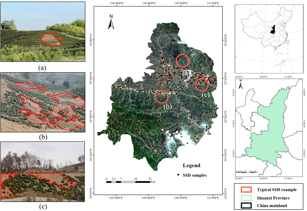
Figure 1. The overview and SSD inventory map of study: (a) Typical SSD example in North area; (b) Typical SSD example in Central area; (c) Typical SSD example in East area.

In response to these challenges, a county-level SSD prediction study was conducted to mitigate the risk of soil disease in the study area.

3 Data resources

3.1 Sample inventory

A comprehensive understanding of the geographical distribution, morphological characteristics, and fundamental information of SSD is indispensable for accurate SSD prediction in the study area (Liu and Hao, 2018). This study identified 415 SSD samples through a combination of field surveys, historical data analysis, and remote sensing interpretation, subsequently vectorizing them into polygon files on the GIS platform. Although the dataset contains only 415 SSD samples, their sufficiency is ensured by integrating multi-source data (remote sensing, field validation, soil survey), and by applying balanced sampling and data augmentation. This approach enhances the representativeness of the dataset despite the limited size. Small or early SSD may be difficult to identify in remote sensing images and field surveys, resulting in insufficient representativeness, which may consequently lead to conservative estimations of SSD occurrence.

Statistical analysis revealed that the maximum planar area of SSD samples in the study area is 609 m², the minimum is 18 m², and the average is 95 m², with irregular shapes. The characteristic attributes of SSD samples, including length, width, and planar area, were assigned to the plots. A total of 281,756 pixels were identified as representing SSD samples, accounting for 0.76% of the study area’s total area. To support subsequent modeling, an equal number (415) of non-SSD samples were randomly selected from non-SSD areas as negative samples, completing the sample database for SSD prediction in the study area (Figure 1).

Equal sampling was employed to balance the dataset under small-sample conditions, but this may not reflect the true distribution of SSD versus non-SSD areas. Future research can adopt more advanced sampling methods, such as SMOTE or weighted loss functions, to address the issue of class imbalance.

3.2 Conditioning factors

At present, research on SSD remains scant, yet this study, informed by field observations and historical data examination, considers three major categories of influencing factors: topographic factors, encompassing slope, aspect, plan curvature, profile curvature, and elevation; environmental factors, including normalized difference vegetation index (NDVI), mean annual precipitation (MAP), and land use type (LUT); and soil factors, comprising soil type, soil texture (ST), soil clay content (SCC), soil organic matter content (SOMC), soil sand content (SSC), soil powder content (SPC), and soil pH (PH), all serving as contributing factors to the onset of SSD. The original data sources utilized in this study are detailed in Table 1.

Table 1

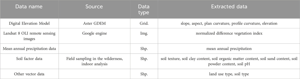
Table 1. Summary of data sources.

3.2.1 Topographic factors

The influence of slope on the occurrence of SSD is complex and multifaceted, closely associated with water distribution and vegetation growth dynamics (Figure 2a). On steep slopes, rainfall is more likely to generate surface runoff, which can exacerbate soil erosion and lead to the onset of SSD (Yuan et al., 2024).

Figure 2

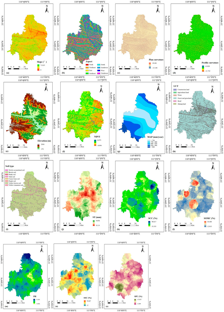
Figure 2. The conditioning factor maps of SSD: (a) Slope; (b) Aspect; (c) Plan curvature; (d) Profile curvature; (e) Elevation; (f) NDVI; (g) MAP; (h) LUT; (i) Soil type; (j) ST; (k) SCC; (l) SOMC; (m) PH; (n) SSC; (o) SPC.

Aspect significantly impacts water distribution, sunlight exposure, and vegetation cover, thereby affecting SSD occurrence (Figure 2b). Sun-exposed slopes are more susceptible to water loss due to higher temperatures, while shaded slopes retain moisture, promoting vegetation growth. Additionally, east-facing and west-facing slopes differ in their solar radiation reception, influencing soil moisture distribution and vegetation patterns (Baiamonte et al., 2019).

Plan curvature (Figure 2c) and profile curvature (Figure 2d) serve as indicators of terrain undulation. In areas with pronounced undulation, uneven water distribution can result in increased soil dryness at higher elevations, heightening SSD risk (Wu et al., 2022).

Elevation also plays a critical role in SSD occurrence. As elevation increases, temperature and atmospheric pressure decrease, leading to lower soil temperatures that can hinder vegetation growth (Amonil et al., 2023). Changes in atmospheric pressure impact evaporation and precipitation, further affecting soil moisture levels. Additionally, variations in elevation can alter soil types, with some high-altitude regions experiencing permafrost conditions that significantly influence soil properties (Figure 2e).

3.2.2 Environmental factors

The Normalized Difference Vegetation Index (NDVI) provides a clear indicator of regional vegetation coverage, making it a key factor influencing SSD (Figure 2f). Higher NDVI values generally indicate healthier vegetation, which can mitigate SSD risk. Conversely, increased precipitation levels can intensify runoff and soil erosion, elevating the likelihood of SSD (Sholagberu et al., 2019). Rainfall plays an essential role in supporting plant growth, and the absence or degradation of vegetation exacerbates SSD occurrences (Figure 2g) (Ke and Zhang, 2022).

Land use type (LUT) significantly affects SSD by influencing soil coverage and conservation. Different land use practices, such as agriculture, forestry, and urbanization, exert varied impacts on soil stability and susceptibility to SSD (Figure 2h).

3.2.3 Soil factors

Soil types vary in their capacities for moisture retention, resistance to weathering, and compatibility with vegetation, all of which directly impact SSD occurrence (Figure 2i). Soil attributes such as texture, organic matter content, and pH play critical roles. Soil texture affects water infiltration and root growth (Figure 2j). Clay content enhances water retention and fertility (Figure 2k), while organic matter stabilizes soil structure and improves fertility (Figure 2l) (Yan and Gao, 2021). Soil pH influences nutrient availability and plant growth, with extremes in acidity or alkalinity potentially hindering vegetation and increasing SSD risk (Figure 2m). Sandy soils are more prone to drying, heightening SSD risk (Figure 2n), whereas higher silt content helps retain moisture, reducing water loss and the likelihood of SSD (Figure 2o) (Moriaque et al., 2019).

3.3 Preparation of input datasets

To reconcile the diverse dimensions and scales of various datasets and avoid data redundancy, the t-Distributed Stochastic Neighbor Embedding (t-SNE) method was applied for dimensionality reduction (Horrocks et al., 2018). Following this, all layers of influencing factors were standardized to a uniform resolution of 30×30 m, resulting in the development of a comprehensive dataset required for model analysis. Subsequently, the dataset underwent K-fold Cross Validation (K-CV) to ensure robustness and reliability. After validation, the data was split into training and validation sets in a 7:3 ratio, with 70% (724 samples) allocated for training the model and 30% (310 samples) reserved for validating the predictive performance of the results (Zafar and Salahuddin, 2009).

4 Methodologies

This study proposes an innovative method for SSD prediction by integrating the Stacked Autoencoder (SAE) with the Dense Residual Network (DRN). Using Shangnan County, Shaanxi Province, China as the study area, the overall technical process is divided into four primary steps: (1) Construction of the SSD-related dataset; (2) Design of the SSD prediction network; (3) Implementation of SSD prediction mapping using the SVM model, CPCNN-RF model, U-Net model, and SAE-DRN model; (4) Evaluation of prediction accuracy, comparing the performance of deep learning networks with traditional machine learning models. The detailed workflow is illustrated in Figure 3.

Figure 3

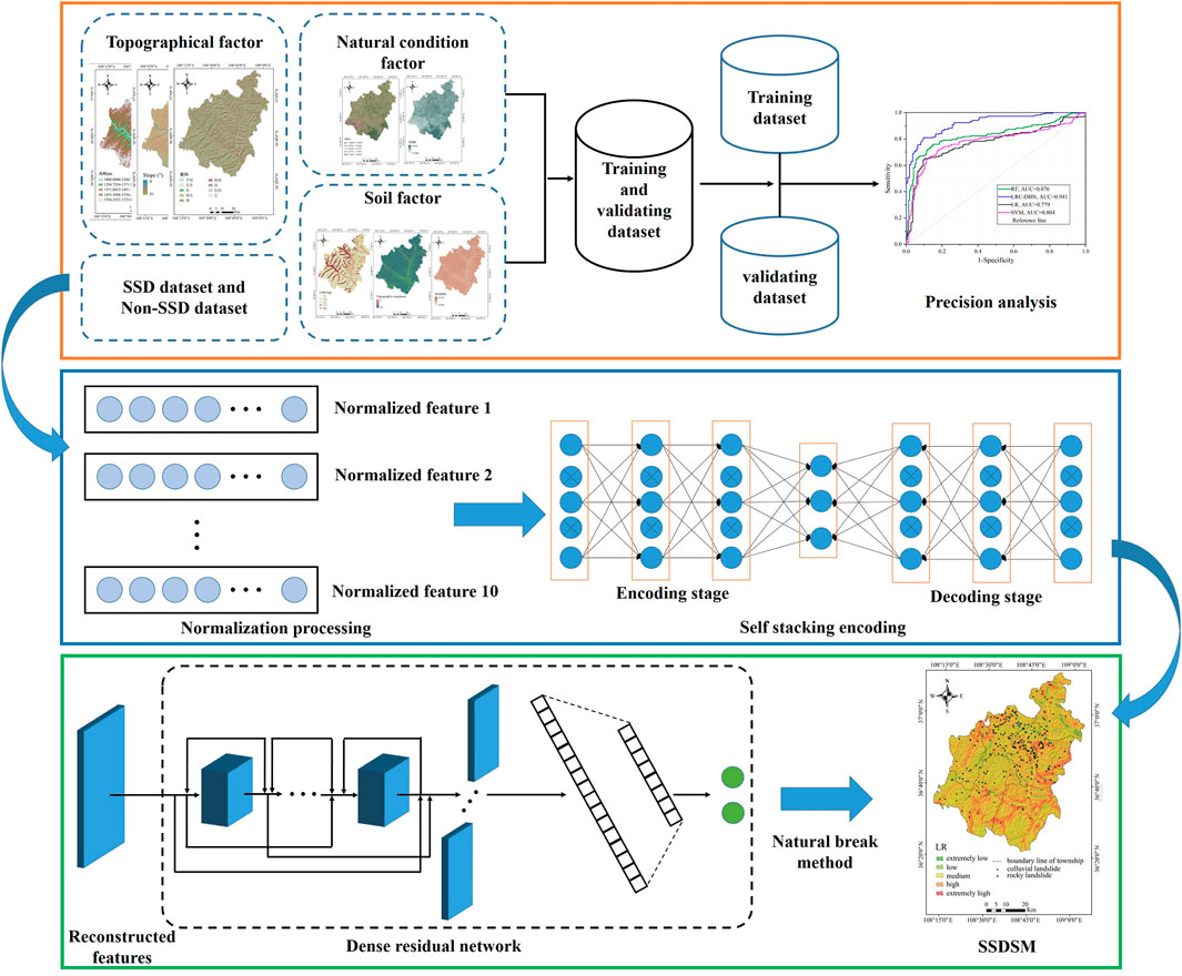
Figure 3. Flowchat of the study.

4.1 Multicollinearity detection method

Machine learning models often operate under the assumption that independent variables are mutually independent. However, as this study adopts a comprehensive approach to selecting factors influencing SSD, it inevitably introduces correlations among these variables. When these correlations become sufficiently strong, the regression coefficient of one variable may increase substantially due to the presence of another, potentially resulting in overfitting or under fitting during model training. This issue, commonly referred to as multicollinearity, can undermine model performance.

To address this, the study employs Pearson correlation coefficients (Pr) and variance inflation factors (VIF) to detect autocorrelation among the influencing factors. The Pearson correlation coefficient (Pr) quantifies the strength of the linear relationship between two factors influencing SSD. Its value ranges from −1 to 1, with values closer to 1 indicating stronger positive correlations, and values closer to −1 indicating stronger negative correlations (Leonenko et al., 2013). The variance inflation factor (VIF) is a statistical measure used to identify the degree of multicollinearity among predictors (Garcia et al., 2015). For each factor X_i influencing SSD, the VIF is calculated as shown in Equation 1.

$\text{VIF}\left({\mathrm{X}}_i\right)=\frac{1}{1-R_i^2}(1)$

In this context, R_i² represents the coefficient of determination for the regression model in which X_i serves as the dependent variable, while the remaining factors act as independent variables. An elevated VIF value denotes a stronger correlation among the factors influencing SSD. When the VIF exceeds 10, it is indicative of significant multicollinearity among these factors. To address this issue, this study adopts an elimination strategy to exclude SSD influencing factors with substantial multicollinearity.

4.2 Contribution calculation of each factors

In prior studies, the use of singular conventional models such as Information Gain Ratio (IGR), Support Vector Machine (SVM), and Random Forest (RF) often overlooked the intrinsic connections between influencing factors and real-world scenarios. Furthermore, these models demonstrated sensitivity to noise and outliers. To address these limitations and align factor selection results more closely with real-world conditions, this study combines RF and SVM to construct the RF-SVM ensemble learning model for factor selection. The principles underlying RF and SVM can be referenced in the literature (Castro-Franco et al., 2015; Borthakur and Dey, 2020). The integration of RF’s ensemble capability with SVM’s robust performance enhances the overall model robustness, reducing susceptibility to noise and outliers while improving performance in high-dimensional data. Using the RF-SVM model, data undergo feature selection and preliminary classification. The model leverages the voting mechanism of multiple trees to bolster robustness, facilitating the calculation of the contribution degree (Cd) of each SSD influencing factor. This process provides a comprehensive assessment of feature importance, offering a more reliable basis for SSD prediction.

4.3 Rough set

Given the unique characteristics of Soil Spotted Degradation (SSD), which involve complex influencing factors and region-specific uncertainties in causative mechanisms, it is essential to construct an objective and reasonable indicator system. This approach enhances the overall framework and methodology of SSD prediction. In predictive assessment, scholars often rely on the empirical knowledge of predecessors to analyze sample characteristics and environmental contexts. Techniques such as collinearity analysis and importance analysis are frequently employed to screen evaluation factors, thereby reducing errors that could affect model predictive accuracy. The Rough Set (RS) method offers a robust approach for addressing the uncertainties in SSD prediction. RS uncovers potential rules within uncertain data, enabling attribute reduction while preserving the classification accuracy of the knowledge base. By leveraging the information in SSD decision tables, RS isolates core attributes critical to prediction, simplifying the cognitive complexity of SSD prediction systems. Additionally, RS minimizes the impact of subjective biases, making it a powerful tool for constructing reliable and efficient SSD predictive models (Swiniarski and Skowron, 2003).

Assuming the domain of discourse is denoted by $\mathrm{U}=\left\{x_1,x_2,\dots ,x_n,\right\}$, where its Attribute Decision Table (ADT) S can be represented by Equation 2.

$\mathrm{S}=〈\mathrm{U},\mathrm{A},\mathrm{V},\mathrm{f}〉(2)$

Herein: $\mathrm{A}=\left\{a_1,a_2,\dots ,a_n,\right\}$ is a non-empty finite set of attributes; $\mathrm{A}=\mathrm{C}\cup \mathrm{D}$; C is the conditional attribute set; D is the decision attribute set; $\mathrm{V}={\mathrm{U}}_{a\in A}{\mathrm{V}}_a$ is the collection of attribute values; ${\mathrm{V}}_a$ represents the range of values for attribute $\mathrm{a}\in \mathrm{A}$; f is the information function, which can be expressed as $\mathrm{f}:\mathrm{U}\times \mathrm{A}\to \mathrm{V}$, then $\mathrm{f}\left(\mathrm{x},\mathrm{a}\right)\in \mathrm{V}$.

The dependency calculation of conditional attribute C on decision attribute D is seen in Equation 3.

$\mathrm{k}={\gamma }_{C\left(D\right)}=\frac{{\text{POS}}_C\left(D\right)}{\left|U\right|}(3)$

Herein: ${\gamma }_{C\left(D\right)}$ represents the ratio of objects that can be classified into decision class $\left.U\right|D$ under the condition attribute C; ${POS}_C\left(D\right)$ represents the positive threshold for D with respect to C.

Not all conditional ADT structures exert a significant impact on the classification results. It is necessary to obtain the minimal relevant attribute set by eliminating redundant attributes. Assuming that the set of all reductions of attribute set A is denoted as Red (A), then the intersection of all reductions core (A) can be represented by Equation 4.

$\text{core}\left(\mathrm{A}\right)=\cap \text{Red}\left(\mathrm{A}\right)(4)$

Due to the differing contributions of conditional attributes to the classification results, it is typically necessary to assess the changes in classification performance before and after attribute selection.

By calculating the difference in dependency between decision attribute D and its subset conditional attribute $B^{\prime }\subseteq B$, the extent of impact $△k$ on the positive threshold $\left.U\right|D$ after removing attribute subset $B^{\prime }$ can be expressed as Equation 5.

$△k=r_B\left(D\right)-r_{B-B^{\prime }}\left(D\right)(5)$

when the value of $△k$ is too small or equals 0, the corresponding attribute is redundant, and it usually needs to be eliminated (Liu et al., 2022).

4.4 Stacked autoencoder (SAE)

Unlike supervised Convolutional Neural Networks (CNNs), autoencoders (AEs), as unsupervised learning artificial neural networks, can learn automatically from large amounts of unlabeled data. By performing nonlinear mappings of input evaluation factors, AEs generate reconstructed data that reveal more intrinsic representations of the input. This process aims to enhance the quality and utility of the data, enabling more effective analysis and predictions (Vincent, 2011).

During the encoding process, the activation function $\mathrm{f}\left(·\right)$ maps the input feature data $\mathrm{x}=\left\{x_1,x_2,\dots ,x_n,\right\}$ to $\mathrm{h}=\left\{h_1,h_2,\dots ,h_m,\right\}$, as shown in Equation 6.

$h=f\left({\mathit{W}}_{y}x+b_y\right)(6)$

Here, W_y represents the weight matrix for mapping $\mathrm{x}=\left\{x_1,x_2,\dots ,x_n,\right\}$ to $\mathrm{h}=\left\{h_1,h_2,\dots ,h_m,\right\}$, and b_y denotes the bias between the input and hidden layers.

In the decoding process, the hidden layer output $\mathrm{h}=\left\{h_1,h_2,\dots ,h_m,\right\}$ is mapped through $\mathrm{g}\left(·\right)$ to obtain the reconstructed output $\mathrm{y}=\left\{y_1,y_2,\dots ,y_n,\right\}$, as shown in Equation 7.

$y=g\left({\mathit{W}}_{z}h+b_z\right)(7)$

Here, W_z represents the weight matrix for mapping $\mathrm{h}=\left\{h_1,h_2,\dots ,h_m,\right\}$ to $\mathrm{y}=\left\{y_1,y_2,\dots ,y_n,\right\}$, and b_z denotes the bias between the output and hidden layers.

The occurrence of SSD is influenced by the impregnating environment and various inducing factors, exhibiting a distinct nonlinear relationship among the characteristic data. A single-layer autoencoder network, however, is insufficient to achieve satisfactory feature extraction. To address this limitation, multiple autoencoders are stacked to form a stacked autoencoder (SAE), as illustrated in Figure 4. SAEs enhance feature representation by leveraging unsupervised learning to extract features from the original training samples. This strengthened representation facilitates more efficient feature fitting in subsequent predictive models.

Figure 4

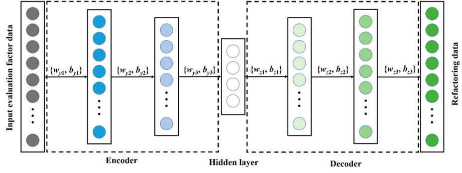
Figure 4. SAE network structure diagram.

4.5 Dense residual network (DRN)

Increasing the depth of CNN networks enables the model to extract deeper data features. However, deepening the network layers often introduces challenges such as gradient explosion and gradient vanishing, which can limit model accuracy. To address these issues, this study incorporates skip connections into the model structure. Skip connections facilitate the explicit fitting of residual mappings rather than the original identity mappings, thereby preserving input information and enhancing gradient propagation efficiency (Cai et al., 2020). The relationship between model input E and output F(E) in residual units can be expressed as Equation 8.

$F\left(E\right)=\psi \left(W_{2}Relu\left(\psi \left(W_1+q_1\right)\right)\right)+q_2(8)$

In the equation, W₁ and W₂ represent the weights of the convolutional layers, q₁ and q₂ denote biases, and $\psi$ signifies batch normalization.

Given the typically limited sample sizes in SSD prediction studies, which can constrain the training accuracy of traditional residual networks, this study constructs a Dense Residual Network (DRN). By employing dense connections that link feature maps from different convolutional layers, the DRN enhances the reuse of SSD feature information within the network. This approach increases the network’s sensitivity to input data and improves model fitting performance. The specific network architecture is depicted in Figure 5.

Figure 5

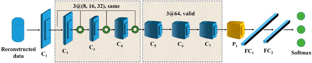
Figure 5. DRN network structure diagram.

4.6 Evaluation methods for results

This study evaluates the precision of SSD prediction using two metrics: Overall Accuracy (OA) and F1 score (Zhou et al., 2024). Additionally, the model’s generalization capability is assessed through the Area Under the Receiver Operating Characteristic Curve (AUC) (Hanley and Mcneil, 1982).

5 Results

5.1 Optimization results of influencing factors

Through multicollinearity analysis and contribution analysis, the suitability of each SSD influencing factor as a variable can be quantitatively assessed. In the multicollinearity analysis (Figure 6), the Pearson correlation coefficients (Pr) between planar curvature, profile curvature, and slope are relatively high, reaching 0.89 and 0.92, respectively, while the Pr values of all other factors are below 0.5. According to the variance inflation factor (VIF) analysis (Table 2), the VIF values of planar curvature and profile curvature are 13.54 and 12.79, respectively, exceeding the threshold of 10, indicating significant multicollinearity. In contrast, the VIF values of all other influencing factors are below 10, and the tolerance (TOL) values are all greater than 0.1, suggesting no multicollinearity issues. The results of the contribution analysis (Figure 7) show that the contribution degrees of all influencing factors are positive, with the soil pH factor having the highest contribution degree at −0.93, followed by the aspect factor (0.85), while the land use type factor has the lowest contribution degree at −0.37.

Figure 6

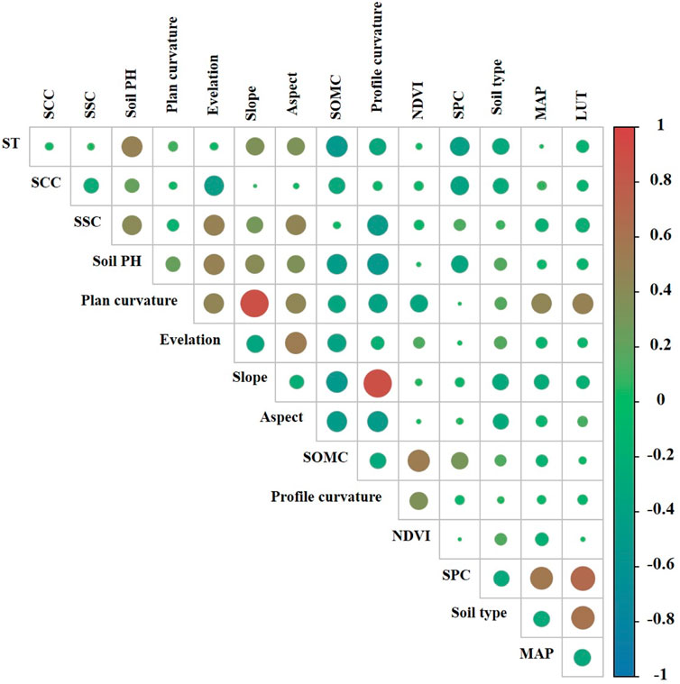
Figure 6. Calculation results of Pr for SSD influencing factor.

Table 2

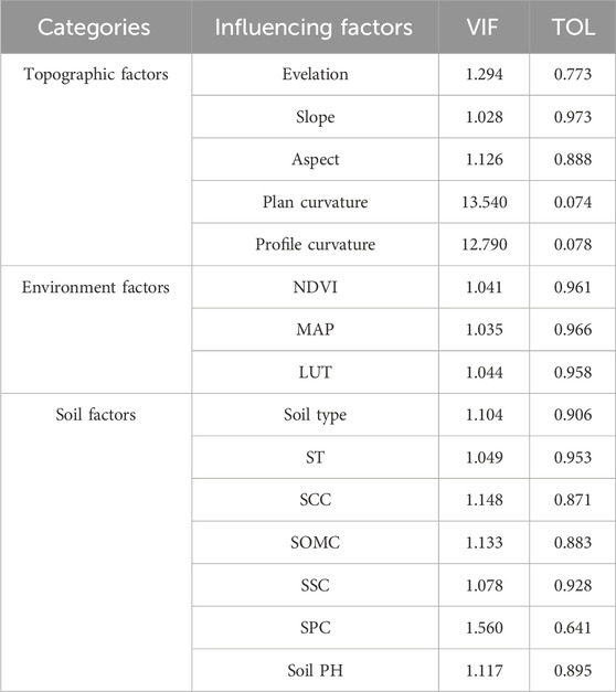
Table 2. VIF and TOL values of influencing factors affecting SSD.

Figure 7

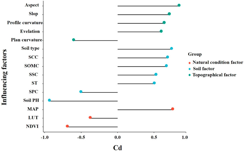
Figure 7. Calculation results of influencing factors affecting SSD.

Considering the comprehensive results of the factor selection process, it is evident that all factors contribute to the model. However, due to the multicollinearity between planar curvature and profile curvature, these two factors will be excluded, and the remaining factors will be retained as input variables for the SSD prediction model.

5.2 Prediction results of SSD

5.2.1 Prediction results of SSD based on machine learning methods

To mitigate the risks of overfitting or underfitting in machine learning model classification due to dataset variations, we employ a 10-fold cross-validation approach to train the SVM model. The posterior probabilities of SSD are normalized to a range between 0 and 1, where a probability close to 1 indicates a higher likelihood of SSD within the assessed unit area. These normalized probabilities are then rasterized in ArcGIS. Using the natural breaks classification method, the predicted outcomes are categorized into five levels: extremely high occurrence area (0.749–0.967), high occurrence area (0.561–0.749), medium occurrence area (0.393–0.561), low occurrence area (0.241–0.393), and extremely low occurrence area (0.001–0.241). This process results in the creation of the SSD Susceptibility Map (SSDSM) based on the SVM model (Figure 8a).

Figure 8

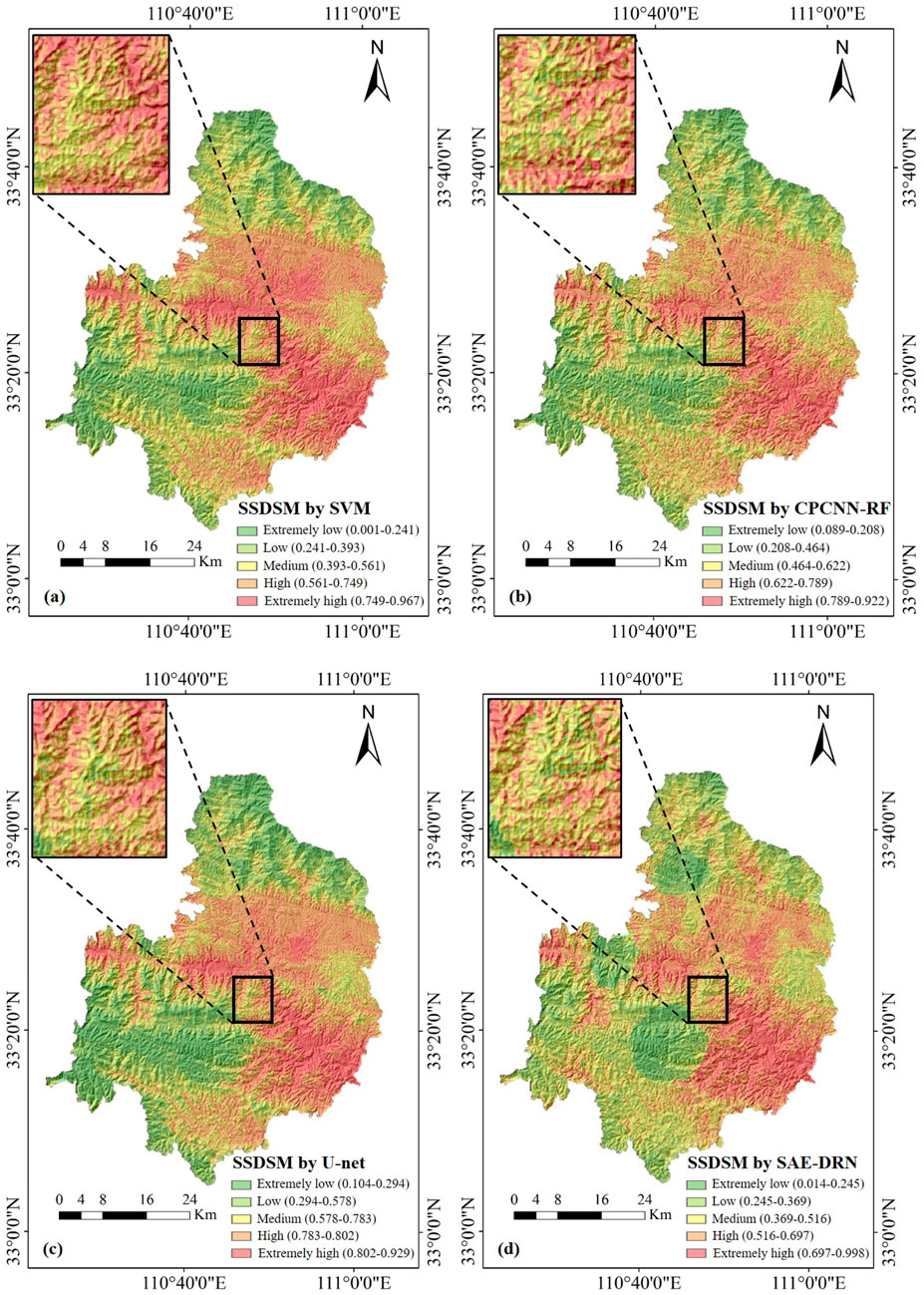
Figure 8. SSDSMs of the study area: (a) SVM; (b) CPCNN-RF; (c) U-net; (d) SAE-DRN.

5.2.2 Prediction results of SSD based on deep learning methods

The deep learning network model eliminates the need for cross-validation by directly utilizing multi-channel pooling layers to extract feature data from the input layers. The model comprises the following four main steps:

1. Shallow Feature Extraction: The first layer, labeled C1, utilizes 8 convolutional kernels of size 3 to filter the reconstructed SSD features, extracting shallow feature information from environmental factors.

2. Residual learning: ① Batch Normalization: This technique is used to restrict output results within a specific range, minimizing the impact of data distribution changes in hidden layers on model performance, thus enhancing stability. ② Dropout Regularization: With a probability of 0.5, this regularization randomly discards hidden layer units, helping to prevent overfitting. Given the complexity of the evaluation factors, the number of convolutional kernels increases with layer depth. Convolutional layers C2, C3, and C4 employ 8, 16, and 32 convolutional kernels, respectively, each with a size of 3. Zero-padding convolution mode (“padding = same”) is applied during training to maintain consistent feature map sizes across layers.

3. Deep Feature Extraction: The feature maps produced by the residual learning module are input into convolutional layers C5, C6, and C7, each with 64 convolutional kernels of size 3, using a valid convolution mode. To reduce computational load, a max-pooling layer P1 with a size of 2 follows C7. The output feature maps from P1 are transformed into one-dimensional vectors and sequentially passed through fully connected layers FC1 (512 neurons) and FC2 (256 neurons), converting the feature data into a 1 × 256 dimensional vector.

4. Softmax Classification: The output layer of the network utilizes a Softmax classifier to classify the data, selecting the category with the highest probability value as the final prediction result and determining the membership of the SSD susceptibility.

This model architecture ensures efficient and precise feature extraction while optimizing performance for SSD prediction. SAE employed three hidden layers (128, 64, 32 neurons), ReLU activation, learning rate 0.001; DRN consisted of 7 convolutional layers (3 × 3 kernels), batch normalization, dropout rate 0.5, Adam optimizer, and learning rate 0.0005. After rough set analysis, the final retained predictors included slope, NDVI, soil pH, soil organic matter content, and land use type, while highly collinear factors such as elevation and precipitation were excluded.

The SSD index was normalized to a range of 0–1 and subsequently rasterized using ArcGIS. Based on the natural breakpoint classification method, the prediction results from the CPCNN-RF, U-Net, and SAE-DRN models were divided into five susceptibility levels: extremely high, high, medium, low, and extremely low occurrence areas. The classification thresholds varied across the models, ranging from 0.089 to 0.998. These classifications facilitated the creation of SSD susceptibility maps for each model (Figures 8b–d), providing a comprehensive visual representation of SSD risk areas. The final statistical analysis of SSD areas, categorized by susceptibility levels, is presented in Figure 11, offering valuable insights into the spatial distribution and extent of SSD risk.

5.3 Evaluation of prediction accuracy

This study assessed the prediction accuracy of SSD models, including SVM, CPCNN-RF, U-Net, and SAE-DRN, using the training dataset alongside Overall Accuracy (OA) and F1 score metrics. As shown in the accuracy evaluation results (Table 3), the SAE-DRN model outperformed the others, achieving the highest OA and F1 values of 0.87 and 0.89, respectively. The CPCNN-RF and U-Net models also demonstrated robust performance, with OA and F1 values exceeding 0.75, reflecting their reliable prediction accuracy. In contrast, the SVM model exhibited lower OA and F1 scores, indicating suboptimal predictive performance.

Table 3

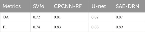
Table 3. Precision analysis table.

Receiver operating characteristic (ROC) curves were generated for the four models using the test dataset (Figure 9). The SAE-DRN model achieved the highest AUC value of 0.92, followed by the CPCNN-RF model (AUC = 0.88) and the U-Net model (AUC = 0.86). In contrast, the SVM model recorded the lowest AUC value. These findings underscore that the SAE-DRN model demonstrates the most robust generalization capacity and delivers superior performance, as confirmed by the comprehensive accuracy evaluation results.

Figure 9

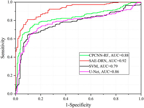
Figure 9. The receiver operating characteristic curves for the four models.

6 Discussion

6.1 Model parameter settings and comparative analysis

During the network training process, fine-tuning the weights by setting appropriate iteration counts is crucial for enhancing the model’s generalization capability. CPCNN-RF and U-Net models were used as baselines. For fairness, CPCNN-RF and U-Net models were re-trained on the same dataset under identical training/testing splits, and hyperparameters were tuned via five-fold cross-validation (Yan et al., 2014; Andrade et al., 2025). Figure 10 presents the training loss and test accuracy curves of the SAE-DRN model across different iterations. When the iteration count was below 500, the classification accuracy remained approximately 0.78. However, the loss value decreased sharply, reflecting continuous model updates. At 600 iterations, the loss value dropped significantly from 0.08 to 0.016 and subsequently stabilized, achieving an optimal classification accuracy of 0.87.

Figure 10

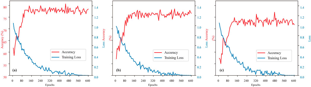
Figure 10. Loss function curve of the training set and classification accuracy curve of the test set under different iteration times: (a) SAE-DRN; (b) CPCNN-RF; (c) U-net.

The SAE-DRN model was trained on an NVIDIA RTX 3090 GPU, requiring approximately 2.8 h for 600 iterations. For comparison, U-Net required 1.9 h and CPCNN-RF required 2.1 h. Although SAE-DRN has slightly higher computational requirements, it is still feasible in practical applications.

We also performed hyper parameter tuning for the CNN-RF and U-Net models. The results revealed that, under the same number of iterations, their classification accuracies were lower than that of the SAE-DRN model. This highlights the superior generalization capability of the SAE-DRN model compared to other deep learning models.

The accuracy assessment of prediction results demonstrated relatively low precision for the SVM model, underscoring the advantage of deep learning in handling nonlinear spatial data for SSD. Both the SAE-DRN and U-Net models achieved higher accuracy, reflecting the efficacy of skip connections in preserving information integrity and mitigating the degradation of accuracy caused by deepening network layers. Building on this, the proposed SAE-DRN model integrates dense connections to enhance data reuse and employs SAE for unsupervised training, thereby strengthening information representation and uncovering deeper insights into influencing factors. This approach partially compensates for the limitations of small sample sizes and yields the best model accuracy.

Moreover, deep learning networks offer distinct advantages: they eliminate the need for dataset preparation or multicollinearity detection, as internal channels inherently address these issues. However, it is important to note that deep learning networks are often sensitive to the sequence of channel inputs. Variations in variable combinations can lead to differences in prediction accuracy and potential overfitting (Muruganantham et al., 2022). Therefore, future research will explore how different combinations of soil spot degradation influencing factors affect prediction accuracy.

6.2 Comparative analysis of SSDSM

The SSD susceptibility maps (SSDSMs) were overlaid with SSD sample data from study area for comparative analysis. Overall, the predictions from the four models exhibited notable similarities. High-risk SSD zones were primarily concentrated in the central-western region, characterized by complex land use patterns, abundant water systems, and heavy rainfall. Recent human engineering activities in this area have further heightened the propensity for SSD. Additionally, this region is near human settlements, with soil predominantly comprising yellow-brown soil exhibiting higher pH levels, indicating a tendency toward alkalinity. This soil condition adversely affects vegetation growth, particularly tea plants (Durdu et al., 2023). As a result, heightened vigilance and proactive SSD control measures are essential in this region.

In the eastern part of study area, SSD occurrences are densely clustered, with all models designating this area as high-risk. The phenomenon follows a horizontal distribution from west to east, influenced by high soil pH, frequent human activity leading to complex land use, and low soil organic matter content. The ecological interpretation of predictors indicates that slope strongly regulates erosion susceptibility, soil pH controls nutrient availability and root development, NDVI reflects vegetation resilience and ground cover, and land use type embodies anthropogenic disturbance. These factors collectively reduce soil fertility, creating conditions conducive to SSD.

6.3 Statistical analysis of SSDSM

The analysis and statistics of the SSD susceptibility maps (SSDSM) include the proportion of different risk zones, the proportion of SSD samples, and the density of SSD samples (Figure 11). Among the predictions from the four models, higher SSD risk correlates with a greater density of SSD samples, with the highest density observed in the high-risk zones. This pattern mirrors the distribution of SSD samples, thereby yielding favorable evaluative outcomes.

Figure 11

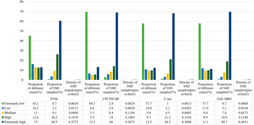
Figure 11. SSDSM statistical analysis chart.

Compared to the SVM model, the deep learning models identified a higher density of SSD samples in high-risk zones, effectively pinpointing target areas for SSD occurrence. Although the CPCNN-RF model classified larger areas as low-risk, it misclassified many SSD samples within these zones. In practical applications, such misclassification may reduce attention to potential disaster areas, potentially misleading disaster prevention strategies (Hosseinpour-Zarnaq et al., 2023).

In contrast, the SAE-DRN model showed a sparser presence of SSD samples in low-risk zones while significantly increasing the density of samples in high-risk zones by 0.1159 pieces/km², 0.0759 pieces/km², and 0.0531 pieces/km². This deep learning model delineated larger low-risk zones and effectively excluded high-risk areas. Additionally, the SAE-DRN model demonstrated higher precision in its coverage of SSD in high-risk zones.

We also selected 30% of the SSD patches from the prediction results for field validation. On-site validation confirmed that all patches predicted as SSD within the study area exhibited soil degradation, demonstrating that the predictive model’s performance meets users’ needs and provides highly reliable results.

In summary, the partitioning results of the SAE-DRN model align closely with actual conditions, contributing positively to soil disease prevention and control efforts. This achievement provides not only valuable guidance for combating soil diseases in tea plantations of the Qinling Mountains in China but also serves as a reference for promoting sustainable agricultural development and ecosystem health management globally. By employing this method, regions facing similar soil degradation challenges can implement predictions and interventions more efficiently.

The study focuses solely on Shangnan County, Shaanxi Province. The model’s performance in regions with differing climatic, topographic, or soil conditions (e.g., tropical or arid zones) remains unverified, noting that further validation is required in different climatic and geomorphic settings (e.g., tropical or arid zones). Meanwhile, the SAE-DRN framework has the potential for transfer learning and promotion applications, but further empirical research is still needed.

7 Conclusion

This study focuses on Shangnan County, Shaanxi Province, China, where SSD influencing factors undergo attribute reduction to select key attributes for constructing an evaluation factor dataset. A SSD susceptibility assessment model, SAE-DRN, which integrates a stacked autoencoder and a dense residual network, is proposed.

A comparative analysis of the SAE-DRN model with the CPCNN-RF model, U-Net model, and SVM model is conducted from the perspectives of SSDSMs, statistical analysis of susceptible regions, and model evaluation accuracy. The experimental results indicate that the SAE-DRN model achieved the highest overall accuracy (OA = 0.87), F1 score (F1 = 0.89), and AUC value (AUC = 0.92), demonstrating superior predictive accuracy and robust performance.

The SAE-DRN model enhances sample feature representation through stacked autoencoders and increases information reuse between convolution layers via a dense residual network. This approach partially mitigates the challenges posed by small sample sizes in SSD prediction. The model effectively captures the nonlinear relationship between SSD occurrences and evaluation factors, improving the accuracy and reliability of SSD predictions.

The study’s SSD prediction results for the study area reveal that land use types, soil types, soil pH, and organic matter content significantly influence SSD occurrence. This provides valuable data to support future tea plantation site selection and soil disease prevention efforts in the region. The research methodology demonstrates exceptional predictive accuracy and reliability, offering a scalable and adaptable solution for soil health management globally.

Data availability statement

The raw data supporting the conclusions of this article will be made available by the authors, without undue reservation.

Author contributions

LZ: Data curation, Project administration, Validation, Resources, Visualization, Methodology, Software, Writing – review and editing, Investigation, Conceptualization, Supervision, Writing – original draft, Funding acquisition. TZ: Writing – review and editing, Methodology, Investigation, Writing – original draft, Data curation. LG: Writing – review and editing, Software, Writing – original draft, Validation, Conceptualization, Visualization.

Funding

The author(s) declare that financial support was received for the research and/or publication of this article. This work was supported by the [Shaanxi Province Youth Science and Technology Rising Star Project] under grant [2025ZC-KJXX-148], [Natural Science Basic Research Program of Shaanxi] under grant [2025JC-YBMS-333, 2025JC-YBMS-334], [Inner scientific research project of Shaanxi Land Engineering Construction Group] under grant [DJNY2024-18, DJNY2024-33], [Internal research projects of Shaanxi Agricultural Development Group] under grant [NFJC2025-55, NFJC2025-56, NFJC2025-57].

Conflict of interest

Authors LZ and TZ were employed by Shaanxi Provincial Land Engineering Construction Group.

The remaining author declares that the research was conducted in the absence of any commercial or financial relationships that could be construed as a potential conflict of interest.

Generative AI statement

The author(s) declare that no Generative AI was used in the creation of this manuscript.

Any alternative text (alt text) provided alongside figures in this article has been generated by Frontiers with the support of artificial intelligence and reasonable efforts have been made to ensure accuracy, including review by the authors wherever possible. If you identify any issues, please contact us.

Publisher’s note

All claims expressed in this article are solely those of the authors and do not necessarily represent those of their affiliated organizations, or those of the publisher, the editors and the reviewers. Any product that may be evaluated in this article, or claim that may be made by its manufacturer, is not guaranteed or endorsed by the publisher.

References

Abdel-Fattah, M. K., Mohamed, E. S., Wagdi, E. M., Shahin, S. A., Alnaimy, M. A., Lasaponara, R., et al. (2021). Quantitative evaluation of soil quality using principal component analysis: the case study of El-Fayoum depression Egypt. Sustainability 13 (4), 1824–1841. doi:10.3390/su13041824

CrossRef Full Text | Google Scholar

Abdo, H. G., Almohamad, H., Dughairi, A. A. A., and Al-Mutiry, M. (2022). GIS-based frequency ratio and analytic hierarchy process for forest fire susceptibility mapping in the Western region of Syria. Sustainability 14 (12), 105–121. doi:10.3390/su14084668

CrossRef Full Text | Google Scholar

Alireza, A., Biswajeet, P., Khalil, R., Mojtaba, Y., Reza, P. H., and Luigi, L. (2018). Spatial modelling of gully erosion using evidential belief function, logistic regression and a new ensemble EBF-LR algorithm. Land Degrad. Dev. 22 (5), 299–308. doi:10.1002/ldr.3151

CrossRef Full Text | Google Scholar

Amonil, P., Jaro, J., Daněk, P., Tikhomirov, D., Novotn, V., Weiblen, G., et al. (2023). Soil erosion affected by trees in a tropical primary rain forest, Papua New Guinea. Geomorphology 425 (9), 108589–108603. doi:10.1016/j.geomorph.2023.108589

CrossRef Full Text | Google Scholar

Andrade, M. G. D. O., Cordeiro, C. F. D. S., Roberto, A. F., Calonego, J. C., and Rosolem, C. A. (2025). Lime and gypsum reduce N-fertilizer requirements and improve soil physics, fertility and crop yields in a double-cropped system. Geoderma 453 (1), 117132–117136. doi:10.1016/j.geoderma.2024.117132

CrossRef Full Text | Google Scholar

Arsyad, A., and Muhiddin, A. B. (2023). Landslide susceptibility mapping for road corridors using coupled InSAR and GIS statistical analysis. Nat. hazards Rev. 12 (5), 657–671. doi:10.1061/NHREFO.NHENG-1499

CrossRef Full Text | Google Scholar

Baiamonte, G., Minacapilli, M., Novara, A., and Gristina, L. (2019). Time scale effects and interactions of rainfall erosivity and cover management factors on vineyard soil loss erosion in the semi-arid area of southern sicily. Water 11 (5), 978–992. doi:10.3390/w11050978

CrossRef Full Text | Google Scholar

Borthakur, N., and Dey, A. K. (2020). Evaluation of group capacity of micropile in soft clayey soil from experimental analysis using SVM-based prediction model. Int. J. geomechanics 20 (3), 04020008–04020017. doi:10.1061/(asce)gm.1943-5622.0001606

CrossRef Full Text | Google Scholar

Cai, Y., Guo, Y., Lang, S., Liu, J., and Hu, S. (2020). Classification of hyperspectral images by spectral-spatial dense-residual network. J. Appl. Remote Sens. 14 (5), 311–320. doi:10.1117/1.jrs.14.036513

CrossRef Full Text | Google Scholar

Castro-Franco, M., Costa, J. L., Peralta, N., and Aparicio, V. (2015). Prediction of soil properties at farm scale using a model-based soil sampling scheme and random forest. Soil Sci. 180 (2), 74–85. doi:10.1097/ss.0000000000000115

CrossRef Full Text | Google Scholar

Chen, Y., Li, M., and Abu Hatab, A. (2020). A spatiotemporal analysis of comparative advantage in tea production in China. Agric. Econ. 7 (12), 66–79. doi:10.17221/85/2020-AGRICECON

CrossRef Full Text | Google Scholar

Costache, R., Hong, H., and Wang, Y. (2019). Identification of torrential valleys using GIS and a novel hybrid integration of artificial intelligence, machine learning and bivariate statistics. CATENA 183 (2), 104179–125. doi:10.1016/j.catena.2019.104179

CrossRef Full Text | Google Scholar

Cota-Ungson, D., González-García, Y., and Juárez-Maldonado, A. (2023). Soil degradation, resilience, restoration, and sustainable use. Agroecol. Approaches Sustain. Soil Manag. 32 (6), 65–82. doi:10.1002/9781119911999.ch4

CrossRef Full Text | Google Scholar

Das, C. R., and Das, S. (2024). Coastal groundwater quality prediction using objective-weighted WQI and machine learning approach. Environ. Sci. Pollut. Res. 9 (13), 31–45. doi:10.1007/s11356-024-32415-w

PubMed Abstract | CrossRef Full Text | Google Scholar

Durdu, B., Gurbuz, F., Koçyiğit, H., and Gurbuz, M. (2023). Urbanization-driven soil degradation; ecological risks and human health implications. Environ. Monit. Assess. 195 (8), 1002. doi:10.1007/s10661-023-11595-x

PubMed Abstract | CrossRef Full Text | Google Scholar

Dyson, J., Mancini, A., Frontoni, E., and Zingaretti, P. (2019). Deep learning for soil and crop segmentation from remotely sensed data. Remote Sens. 11 (16), 1859–1871. doi:10.3390/rs11161859

CrossRef Full Text | Google Scholar

Falah, F., and Zeinivand, H. (2019). GIS-based groundwater potential mapping in khorramabad in Lorestan, Iran, using frequency ratio (FR) and weights of evidence (WoE) models. Water Resour. 46 (5), 633–649. doi:10.1134/S0097807819050051

CrossRef Full Text | Google Scholar

Feng, S., Zhao, W., Yan, J., Xia, F., and Pereira, P. (2024). Land degradation neutrality assessment and factors influencing it in China's arid and semiarid regions. Sci. Total Environ. 925 (15), 171735. doi:10.1016/j.scitotenv.2024.171735

PubMed Abstract | CrossRef Full Text | Google Scholar

Garcia, C. B., Salmeron, R., and Martin, M. M. J. L. (2015). Collinearity: revisiting the variance inflation factor in ridge regression. J. Appl. Statistics 8 (2), 77–84. doi:10.1080/02664763.2014.980789

CrossRef Full Text | Google Scholar

Grunwald, S., Yu, C., and Xiong, X. (2015). Transferability and scaling of soil total carbon prediction models in Florida. Peerj 16 (3), 801–822. doi:10.7287/peerj.preprints.494v1

CrossRef Full Text | Google Scholar

Gu, T., Li, J., Wang, M., and Duan, P. (2022). Landslide susceptibility assessment in Zhenxiong County of China based on geographically weighted logistic regression model. Geocarto Int. 37, 4952–4973. doi:10.1080/10106049.2021.1903571

CrossRef Full Text | Google Scholar

Hanley, J. A., and Mcneil, B. J. (1982). The meaning and use of the area under a receiver operating characteristic (ROC) curve. Radiology 143 (1), 29–36. doi:10.1148/radiology.143.1.7063747

PubMed Abstract | CrossRef Full Text | Google Scholar

Horrocks, T., Holden, E. J., Wedge, D., Wijns, C., and Fiorentini, M. (2018). Geochemical characterisation of rock hydration processes using t-SNE. Comput. and Geosciences 124 (12), 46–57. doi:10.1016/j.cageo.2018.12.005

CrossRef Full Text | Google Scholar

Hosseinpour-Zarnaq, M., Omid, M., Sarmadian, F., and Ghasemi-Mobtaker, H. (2023). A CNN model for predicting soil properties using VIS–NIR spectral data. Environ. Earth Sci. 82 (16), 382–397. doi:10.1007/s12665-023-11073-0

CrossRef Full Text | Google Scholar

Jiajun, L., Gongwen, W., Shuai, Z., Yazhou, S., Jiayu, X., Nie, M., et al. (2017). GIS prospectivity mapping and 3D modeling validation for potential uranium deposit targets in shangnan district, China. J. Afr. earth Sci. 128 (4), 161–175. doi:10.1016/j.jafrearsci.2016.12.001

CrossRef Full Text | Google Scholar

Jiang, X., Wang, H., Zakari, S., Zhu, X., Singh, A. K., Lin, Y., et al. (2023). Assessing the impact of forest conversion to plantations on soil degradation and forest water conservation in the humid tropical region of southeast Asia: implications for forest restoration. Geoderma 440 (10), 116712. doi:10.1016/j.geoderma.2023.116712

CrossRef Full Text | Google Scholar

Kan, J. C., Ferreira, C. S. S., Destouni, G., Haozhi, P., Passos, M. V., Barquet, K., et al. (2023). Predicting agricultural drought indicators: ML approaches across wide-ranging climate and land use conditions. Ecol. Indic. 154, 110524. doi:10.1016/j.ecolind.2023.110524

CrossRef Full Text | Google Scholar

Ke, Q., and Zhang, K. (2022). Interaction effects of rainfall and soil factors on runoff, erosion, and their predictions in different geographic regions. J. Hydrology 22 (7), 605–622. doi:10.1016/j.jhydrol.2021.127291

CrossRef Full Text | Google Scholar

Keshavarzi, A., Tuffour, H. O., Bagherzadeh, A., Tattrah, L. P., Rodrigo-Comino, J., Gholizadeh, A., et al. (2020). Using fuzzy-AHP and parametric technique to assess soil fertility status in northeast of Iran. J. Mt. Sci. 17 (4), 931–948. doi:10.1007/s11629-019-5666-6

CrossRef Full Text | Google Scholar

Khaki, S., Wang, L., and Archontoulis, S. V. (2020). A CNN-RNN framework for crop yield prediction. Front. Plant Sci. 10 (10), 1750–1766. doi:10.3389/fpls.2019.01750

PubMed Abstract | CrossRef Full Text | Google Scholar

Leonenko, N. N., Meerschaert, M. M., and Sikorskii, A. (2013). Correlation structure of fractional pearson diffusions. Comput. Math. Appl. 66 (5), 737–745. doi:10.1016/j.camwa.2013.01.009

PubMed Abstract | CrossRef Full Text | Google Scholar

Liu, Y., and Hao, Y. (2018). Use of remote sensing, GIS and C++ for soil erosion assessment in the Shakkar River basin, India. Sci. Total Environ. 45 (8), 3022–3037. doi:10.1016/j.scitotenv.2018.07.062

CrossRef Full Text | Google Scholar

Liu, P., Ahmad, S., Abdullah, S., and Al-Shomrani, M. M. (2022). A new approach to three-way decisions making based on fractional fuzzy decision-theoretical rough set. Int. J. Intelligent Syst. 37 (3), 2428–2457. doi:10.1002/int.22779

CrossRef Full Text | Google Scholar

Lixi, Z., Pengbo, S., Fang, J., Hengqing, Q., Shumei, R., Yunkai, L., et al. (2013). Using monitoring data of surface soil to predict whole crop-root zone soil water content with PSO-LSSVM, GRNN and WNN. Earth Sci. Inf. 10 (1), 274–292. doi:10.1007/s12145-013-0130-6

CrossRef Full Text | Google Scholar

Maximilian, B., Hauzenberger, C. A., and Yunpeng, D. (2020). Multistage metamorphic evolution of retrograded eclogites from the songshugou complex, qinling orogenic Belt, China. J. Petrology 14 (11), 11–30. doi:10.1093/petrology/egaa007

CrossRef Full Text | Google Scholar

Moriaque, A. T., Félix, K. A., Pascal, H., Anastase, A. H., Socrate, A. M., and Sidoine, B. T. (2019). Factors influencing soil erosion control practices adoption in centre of the Republic of Benin: use of multinomial logistic. J. Agric. Sci. 46 (17), 701–715. doi:10.5539/JAS.V11N17P110

CrossRef Full Text | Google Scholar

Muruganantham, P., Wibowo, S., Grandhi, S., Samrat, N. H., and Islam, N. (2022). A systematic literature review on crop yield prediction with deep learning and remote sensing. Remote Sens. 14 (9), 1990. doi:10.3390/rs14091990

CrossRef Full Text | Google Scholar

Pham, Q. B., Yacine, A., Ali, S. A., Parvin, F., Vojtek, M., Vojteková, J., et al. (2021). A comparison among fuzzy multi-criteria decision making, bivariate, multivariate and machine learning models in landslide susceptibility mapping. Geomatics, Nat. Hazards Risk 12 (1), 1741–1777. doi:10.1080/19475705.2021.1944330

CrossRef Full Text | Google Scholar

Pournader, M., Hasan, A., Feiznia, S., Haji, K., and Peirovan, H. R. (2018). Spatial prediction of soil erosion susceptibility: an evaluation of the maximum entropy model. Earth Sci. Inf. 11 (3), 1132–1147. doi:10.1007/s12145-018-0338-6

CrossRef Full Text | Google Scholar

Raghubanshi, S., Agrawal, R., Rajawat, A., and Rajak, D. R. (2023). Semi-automatic extraction of land degradation processes using multi sensor data by applying object based classification technique. Appl. Geomatics 15 (1), 239–248. doi:10.1007/s12518-023-00503-0

CrossRef Full Text | Google Scholar

Rao, W., Shen, Z., and Duan, X. (2023). Spatiotemporal patterns and drivers of soil erosion in Yunnan, southwest China: RULSE assessments for recent 30years and future predictions based on CMIP6. CATENA 36 (4), 319–333. doi:10.1016/j.catena.2022

CrossRef Full Text | Google Scholar

Razavi-Termeh, S. V., Sadeghi-Niaraki, A., and Choi, S. M. (2020). Ubiquitous GIS-based forest fire susceptibility mapping using artificial intelligence methods. Remote Sens. 12 (10), 1689–1697. doi:10.3390/rs12101689

CrossRef Full Text | Google Scholar

Rukhovich, D. I., Koroleva, P. V., Rukhovich, D. D., and Rukhovich, A. D. (2022). Recognition of the bare soil using deep machine learning methods to create maps of arable soil degradation based on the analysis of multi-temporal remote sensing data. Remote Sens. 14 (9), 2224. doi:10.3390/rs14092224

CrossRef Full Text | Google Scholar

Saha, A., Pal, S. C., Chowdhuri, I., Islam, A. R. M. T., Roy, P., and Chakrabortty, R. (2022). Land degradation risk dynamics assessment in red and lateritic zones of eastern plateau, India: a combine approach of K-fold CV, data mining and field validation. Ecol. Inf. 69 (7), 101653. doi:10.1016/j.ecoinf.2022.101653

CrossRef Full Text | Google Scholar

Sholagberu, A., Mustafa, M. U., Yusof, K., Hashim, A., and Isa, M. (2019). Multivariate logistic regression model for soil erosion susceptibility assessment under static and dynamic causative factors. Pol. J. Environ. Stud. 28 (5), 22–35. doi:10.15244/pjoes/91943

CrossRef Full Text | Google Scholar

Swiniarski, A. R. W., and Skowron, B. A. (2003). Rough set methods in feature selection and recognition. Pattern Recognit. Lett. 24 (6), 833–849. doi:10.1016/s0167-8655(02)00196-4

CrossRef Full Text | Google Scholar

Vincent, P. (2011). A connection between score matching and denoising autoencoders. Neural Comput. 23 (7), 1661–1674. doi:10.1162/neco_a_00142

PubMed Abstract | CrossRef Full Text | Google Scholar

Wang, Y., Wen, H., Sun, D., and Li, Y. (2021). Quantitative assessment of landslide risk based on susceptibility mapping using random forest and GeoDetector. Remote Sens. 13 (13), 2625–2637. doi:10.3390/rs13132625

CrossRef Full Text | Google Scholar

Wu, Y., Ke, Y., Chen, Z., Liang, S., and Hong, H. (2020). Application of alternating decision tree with AdaBoost and bagging ensembles for landslide susceptibility mapping. CATENA 187 (1), 104396–396. doi:10.1016/j.catena.2019.104396

CrossRef Full Text | Google Scholar

Wu, J., Cheng, Y., Mu, Z., Dong, W., Zheng, Y., Chen, C., et al. (2022). Temporal spatial mutations of soil erosion in the middle and lower reaches of the lancang River Basin and its influencing mechanisms. Sustainability 14 (1), 5169–3764. doi:10.3390/su14095169

CrossRef Full Text | Google Scholar

Xie, W., Nie, W., Saffari, P., Robledo, L., Descote, P.-Y., and Jian, W. (2021). Landslide hazard assessment based on Bayesian optimization-support vector machine in Nanping City, China. Nat. Hazards 26 (7), 931–948. doi:10.1007/s11069-021-04862-y

CrossRef Full Text | Google Scholar

Xue, W., Peng, C., Chen, H., Wang, H., Yang, W., Yang, Y., et al. (2018). Nitrous oxide emissions from three temperate forest types in the Qinling Mountains, China. J. For. Res. 11 (6), 1417–1427. doi:10.1007/s11676-018-0721-7

CrossRef Full Text | Google Scholar

Yan, R., and Gao, J. (2021). Key factors affecting discharge, soil erosion, nitrogen and phosphorus exports from agricultural polder. Ecol. Model. 452 (1), 109586–584. doi:10.1016/j.ecolmodel.2021.109586

CrossRef Full Text | Google Scholar

Yan, C., Liu, E., and Shu, F. (2014). Review of agricultural plastic mulching and its residual pollution and prevention measures in China. J. Agric. Resour. Environ. 22 (6), 277–292. doi:10.13254/j.jare.2013.0223

CrossRef Full Text | Google Scholar

Yang, L., Zhao, G., Mu, X., Lan, Z., Jiao, J., An, S., et al. (2023). Integrated assessments of land degradation on the Qinghai-Tibet plateau. Ecol. Indic. 147 (3), 109945. doi:10.1016/j.ecolind.2023.109945

CrossRef Full Text | Google Scholar

Yousefi, S., Pourghasemi, H. R., Avand, M., Janizadeh, S., Tavangar, S., and Santosh, M. (2021). Assessment of land degradation using machine-learning techniques: a case of declining rangelands. Land Degrad. Dev. 32 (3), 1452–1466. doi:10.1002/ldr.3794

CrossRef Full Text | Google Scholar

Yuan, S., Xu, Q., Zhao, K., Zhou, Q., Wang, X., Zhang, X., et al. (2024). Dynamic analyses of soil erosion and improved potential combining topography and socio-economic factors on the Loess Plateau. Ecol. Indic. 160 (11), 111814–1071. doi:10.1016/j.ecolind.2024.111814

CrossRef Full Text | Google Scholar

Zafar, M., and Salahuddin, K. (2009). On the use of K-Fold cross-validation to choose cutoff values and assess the performance of predictive models in stepwise regression. Int. J. Biostats 5 (1), 25–26. doi:10.2202/1557-4679.1105

CrossRef Full Text | Google Scholar

Zalidis, G. (2020). Employing a multi-input deep convolutional neural network to derive soil clay content from a synergy of multi-temporal optical and radar imagery data. Remote Sens. 12 (7), 2075–2084. doi:10.3390/rs12091389

CrossRef Full Text | Google Scholar

Zhou, W., Yu, R., Guo, F., Shen, C., Liu, Y., and Huang, Y. (2024). Source apportionment and risk assessment of soil heavy metals in the Huangshui River Basin using a hybrid model. Ecol. Indic. 160 (24), 111906–114018. doi:10.1016/j.ecolind.2024.111906

CrossRef Full Text | Google Scholar