Comparative modeling of nitrogen losses in a tile-drained watershed using SWAT model: uncertainty and calibration considerations

Ecohydrological models are critical for understanding coupled hydrologic–biogeochemical processes in tile-drained watersheds and for assessing management options. Despite recent advances in SWAT’s hydrological and biogeochemical processes, there has been limited evaluation of both the original and new tile drainage and nitrogen (N) modules. We therefore applied a comparative modeling approach in a typical Midwestern tile-drained watershed, evaluating eight configurations that vary tile-drainage module (original/new), tile parameter treatment (calibrated/default), and N module (original/new) to assess performance for N-loss simulation. Using daily streamflow and nitrate (NO₃ ⁻) load records from three monitoring sites, we conducted calibration, validation, sensitivity analysis, and uncertainty assessment. Each configuration effectively reproduced daily and monthly dynamics, although high-flow and associated NO₃ ⁻ load peaks were underestimated. We found that the new tile module generally improved streamflow simulations, particularly under tile parameter calibration conditions, while the new N module consistently enhanced NO₃ ⁻ load simulations compared to the original module. Despite improvements in streamflow and NO₃ ⁻ loads with the new tile and N modules, the additional processes in the new N module can magnify uncertainty in N-gas-flux estimates when calibration observations are scarce. We recommend applying the new N module in conjunction with additional measurements—such as soil moisture and nitrous oxide (N₂O) fluxes—to constrain better N gas flux estimates beyond outlet NO₃ ⁻ load data. If such observations are unavailable, careful calibration with reasonable estimates may still help constrain soil N cycling and improve overall N budget accuracy.

1 Introduction

Tile drainage is a prevalent agricultural practice in the Midwest USA, particularly in regions characterized by flat topography and clayey soils that impede natural drainage (Skaggs et al., 1994; Moriasi et al., 2012). This system, which involves the installation of subsurface drainage pipes, aims to enhance soil aeration and crop productivity by managing excess water levels (Skaggs et al., 1994; Schilling and Helmers, 2008). However, while tile drainage effectively alleviates waterlogging and improves agricultural yields, it also poses significant environmental challenges (Baker and Johnson, 1977; Logan et al., 1994). Tile drainage significantly influences streamflow and nutrient transport by modifying hydrological pathways and nutrient cycling processes (Li et al., 2010; Crossman et al., 2014). Compared to non-tiled systems, tile-drained watersheds exhibit distinct distributions of water balance components, including surface runoff, lateral flow, shallow groundwater flow, and aquifer recharge (Schilling and Helmers, 2008; May et al., 2023). Additionally, tile drainage affects water quality by reducing surface runoff and erosion, increasing soil aeration—which promotes mineralization but limits denitrification—and enhancing nitrate (NO₃ ⁻) leaching into surface waters (Ikenberry et al., 2017; Ford et al., 2018).

In the Midwest, where intensive agriculture and heavy fertilizer use are common, the risk of NO₃ ⁻ leaching is significantly elevated (Dinnes et al., 2002). Research indicates that tile drainage systems accelerate NO₃ ⁻ transport from agricultural fields to surface waters, raising water quality and public health concerns (Zucker and Brown, 1998). Beyond nitrogen (N) loss to freshwater systems, tile drainage also influences N gas fluxes, including ammonia volatilization (NH₃) and fluxes of nitrous oxide (N₂O), nitric oxide (NO), and dinitrogen (N₂), contributing to environmental concerns (Gu et al., 2013; Nash et al., 2015). The interactions between tile drainage, N cycling, and hydrological processes are complex and influenced by factors such as soil moisture, temperature, and fertilizer application timing and rates (Burton et al., 2024). A comprehensive understanding of N loss dynamics in tile-drained systems is essential for developing effective management strategies that minimize environmental impacts while maintaining agricultural productivity (Awale et al., 2015). Key priorities include investigating the mechanisms driving NO₃ ⁻ leaching and N gas fluxes, their environmental consequences, and potential mitigation strategies (Hama-Aziz et al., 2017; Fabrizzi et al., 2024).

Ecohydrological models play a key role in simulating watershed hydrology, identifying and quantifying N-loss pathways, and guiding the development of effective BMPs for tile-drained systems (Moridi, 2019; Ghimire et al., 2020; Wang et al., 2021b; Yousefi and Moridi, 2022). By integrating hydrologic, soil, and nutrient-cycling processes, they capture the coupled hydrologic–biogeochemical interactions that govern N transport (Groffman et al., 2009; Wang et al., 2021a; Chen et al., 2024). The Soil and Water Assessment Tool (SWAT), a leading watershed-scale ecohydrological model, is widely used to test management scenarios under varying conditions and to pinpoint strategies that reduce N losses. (Arnold et al., 1998). By accurately simulating N transport and transformation in agricultural systems, SWAT provides valuable insights into the effects of land management decisions on water quality and soil health (Nazari Mejdar et al., 2023). The SWAT model’s representation of tile drainage systems and nutrient cycling processes has undergone progressive development over time. Initially, a simple tile drainage module was introduced (Du et al., 2005; Du et al., 2006), followed by the development of a more physically-based tile drainage module (Moriasi et al., 2012; Moriasi et al., 2013b). Both modules have been successfully applied in field- and watershed-scale studies, enhancing SWAT’s capability to simulate subsurface drainage dynamics. For N cycling, SWAT’s original soil N mineralization algorithm integrates immobilization, making it a net mineralization model (Seligman and Keulen, 1980). The model also incorporates ammonia volatilization and nitrification (Reddy et al., 1979) and accounts for NO₃ ⁻ loss through denitrification (Neitsch et al., 2011). Acknowledging the close interconnection between soil carbon (C) and N cycling, recent advancements in the SWAT model have enhanced its capability to simulate soil organic C dynamics and N gas fluxes using the Century/DayCent model algorithms (Zhang et al., 2013; Yang et al., 2017; Liang et al., 2022; Liang et al., 2023; Tijjani et al., 2023; Tijjani et al., 2024). These enhancements could potentially increase SWAT’s effectiveness in evaluating the impacts of tile drainage on N losses through various pathways, thereby improving its applicability in managing agricultural watersheds and conducting water quality studies.

Since model prediction uncertainty largely stems from input data, model structure, and model parameters (Refsgaard et al., 2006; Abbaspour K. et al., 2007; Abbaspour K. C. et al., 2007; Abbaspour, 2013), adding more biogeochemical processes can increase uncertainty. While incorporating extensive field observations is required to constrain parameters and reduce uncertainty (Herrera et al., 2022), large-scale data collection is often lacking. In such cases, soft/estimated data provide a practical alternative for improving model calibration (Arnold et al., 2015; Nelson et al., 2018). Despite advances in simulating tile drainage and N cycling, comparative evaluations of different SWAT versions remain scarce—particularly regarding their representation of N cycling within tile-drained systems. Comparative assessments of model versions and/or configurations offer several key benefits: 1) Identifying model strengths and weaknesses across different configurations, improving model selection for specific research and management objectives and/or applications (Kujawa et al., 2020). 2) Improving our understanding of model uncertainty, especially regarding how different representations of processes affect the predictions of flow pathways and N losses (Narsimlu et al., 2015). And 3) Refining model calibration approaches by determining the types and resolutions of data needed for accurate parameterization (Perrin et al., 2001). To date, no studies have simultaneously evaluated the new and original SWAT tile drainage and N modules, and comprehensive comparisons between the updated and original versions remain largely absent. Therefore, the main objective of this study, and a novel contribution, is a comparative modeling evaluation of SWAT’s ability to simulate N losses in a typical Midwestern tile-drained watershed using eight configurations spanning tile drainage module (original/new), tile-parameter treatment (calibrated/default), and N module (original/new). Overall, we aimed to identify the key module structures and processes that most significantly contribute to prediction uncertainty, and to determine the additional observational and/or soft data needed to improve model calibration and accuracy.

2 Materials and methods

2.1 Study area and data collection

The Iowa’s South Fork of the Iowa River Watershed (SFW; Figure 1) encompasses an area of 775 km², including the tributaries of South Fork (containing Tipton Creek) and Beaver Creek (Figure 2c; Supplementary Table S3). It serves as a representative example of the Des Moines Lobe, the primary landform region in north-central Iowa. The terrain is relatively young, having developed approximately 10,000 years after the last glacial retreat, resulting in natural stream incision and alluvial valley formation primarily in the lower sections of the watershed (Figure 2a). The region’s soils are highly productive, dominated by the Clarion-Nicollet-Webster soil association, which consists of a sequence of well-drained Typic Hapludolls, somewhat poorly drained Aquic Hapludolls, and poorly drained Typic Haplaquolls (Tomer et al., 2008b). The average annual precipitation in the SFW during the study period (2001–2018) was 894 mm, with approximately 62% falling during the growing season. The daily temperature can drop to as low as −13 °C in January and rise to as high as 29 °C in July (Bailey et al., 2022). Currently, corn and soybean rotations cover approximately 85% of the land area (Figure 2b), and animal feeding operations, primarily for swine, are prevalent, particularly in the Tipton Creek catchment (Tomer et al., 2008a).

Figure 1

Figure 1. Location of the South Fork of the Iowa River Watershed (SFW) and the Kelley experimental site in Iowa.

Figure 2

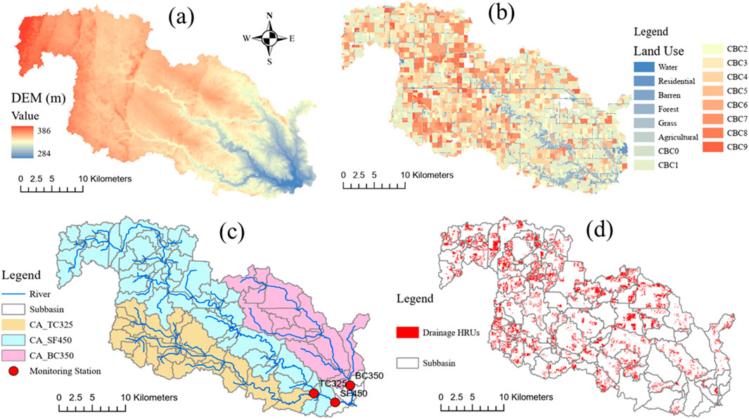
Figure 2. The South Fork of the Iowa River Watershed (SFW) maps of (a) DEM, (b) Land use (see Supplementary Table S1 for explanation), (c) Control areas of monitoring stations (see Supplementary Table S3), and (d) HRUs setup with tile drainage distributed in subbasins.

Cropping rotations were determined using annual classified satellite data made available by the USDA National Agricultural Statistics Service (NASS). Ten years of NASS crop-cover data (2000–2009) were overlaid to identify dominant crop rotations occurring on crop lands in the watershed (Supplementary Table S1). Crop lands were identified using digitized agricultural field boundaries within the watershed obtained from local Farm Service Agency (USDA-FSA) offices. Non-crop land was dominantly hay and wetland forest, which were typically located in riparian valleys. Roadways, farmsteads, and towns were classified as residential land. The management schedules for corn and soybean are presented in Supplementary Table S2, based on the information provided by Tomer et al. (2008a).

Artificial drainage was installed to allow agricultural production, beginning more than 100 years ago. Although the location of individual drains in fields has not been mapped, previous studies have estimated that up to 80% of the watershed may be artificially drained (Green et al., 2006). Approximately 35% of the watershed’s soils are classified as well-drained, but most are present on steeper slopes that are not farmed or are surrounded by poorly drained soils. The drainage districts tend to coincide with the watershed subbasins where poorly drained soils are common. This estimated value includes all of the soils that are not well drained and a few that are well drained but are surrounded by poorly drained soil.

Three stream gauging stations were utilized to provide long-term observations of daily streamflow and NO₃ ⁻ load (Supplementary Table S3). These stations monitor the three major tributaries: South Fork (USGS#05451210, near New Providence), Tipton Creek, and Beaver Creek (Figure 2c). Detailed methodologies for streamflow monitoring and water sampling can be found in Tomer et al. (2008b). Nitrate concentrations in our dataset were estimated using linear interpolation between samples collected at least weekly. Sampling included weekly point samples taken in the thalweg and automated composite samples collected during runoff events using a peristaltic pump. A computerized data logger controlled the composite sampler, triggering flow-paced sampling based on the site’s rating curve, with one composite sample analyzed per event. The weekly and event-based sample results were integrated into a time-series management system, which applied linear interpolation to generate a 10-min resolution concentration record. This high-resolution time series was then used to calculate daily mean concentrations, which served as the basis for daily NO₃ ⁻ load estimates (i.e., concentration × daily total stream flow).

2.2 The development of tile drainage and N cycling processes for SWAT

The SWAT model is the most widely used watershed-scale ecohydrological model globally for evaluating water quantity and quality affected by land use and management practices. It can simulate tile drainage systems using both a simplified tile module and a more physically based module. While the SWAT model has been employed for tile drainage simulations, its application to NO₃ ⁻ loss through tile systems has rarely been reported. The model’s original soil N mineralization processes were based on the PAPRAN model (Seligman and Keulen, 1980), which incorporates immobilization, making it a net mineralization algorithm. It considers fresh organic N and two humic N pools (active and stable). Mineralized N is directly added to the NO₃ ⁻ pool, while ammonium (NH₄ ⁺) is introduced into the soil system through fertilization, which can then be lost via ammonia volatilization and nitrification, using methods developed by Reddy et al. (1979). The original SWAT model also calculates NO₃ ⁻ loss through denitrification, incorporating a threshold for nutrient cycling water factors necessary for denitrification to occur (Neitsch et al., 2011). To ascertain the amount of NO₃ ⁻ transported with water, the concentration of NO₃ ⁻ in the mobile water is first calculated, which is then multiplied by the volume of water moving through the tile drainage pathway to determine the mass of NO₃ ⁻ lost from the soil layer containing the tile.

Recognizing the close interconnection between soil C and N cycling processes, recent advancements in the SWAT model enhance its ability to simulate soil organic C dynamics and N gas fluxes (Zhang et al., 2013; Yang et al., 2017; Liang et al., 2022; Liang et al., 2023; Tijjani et al., 2023; Tijjani et al., 2024). These improvements make it more applicable for studies on water quality, soil health, and BMPs assessment. Below, we briefly outline these advancements and highlight how the updated model differs from the original version.

2.2.1 The new soil N module

The core algorithms for C and N cycling processes from the Century model (Parton et al., 1994; Izaurralde et al., 2006) have been modified and integrated into the SWAT model to enable a more comprehensive simulation of soil C and N dynamics within the soil profile (Figure 3) (Zhang et al., 2013). Furthermore, DayCent-based N₂O production and fluxes (Del Grosso et al., 2000; Parton et al., 2001) have also been incorporated into the SWAT model (Figure 3) (Yang et al., 2017). Thus, this enhanced SWAT model simulates N cycling processes within an agroecosystem by incorporating key steps like N fixation, mineralization, nitrification, denitrification, plant uptake, and leaching, allowing it to track the movement of N through different soil pools and between the atmosphere, vegetation, and soil, with a particular focus on the daily dynamics of these processes. Comprehensive details on soil C and N cycling processes and validation of the enhanced SWAT model are available in related studies (Parton et al., 1994; Izaurralde et al., 2006; Zhang et al., 2013; Liang et al., 2022; Liang et al., 2023; Tijjani et al., 2023; Luo et al., 2024; Tijjani et al., 2024).

Figure 3

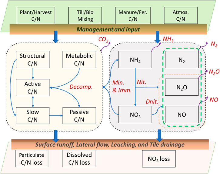
Figure 3. Schematic diagram for Century/DayCent-based soil organic C/N decomposition/mineralization/immobilization and N gas flux algorithms integrated in SWAT.

In comparison to the original N module in SWAT (Neitsch et al., 2011), the new N module is significantly more complex, featuring additional parameters that simulate N₂O fluxes resulting from both nitrification and denitrification processes (Figure 3; Table 1). The new N module also simulates the production of NO and N₂ as byproducts of the nitrification and denitrification reaction sequence (Figure 3). Detailed information on N gas fluxes simulation refers to Yang et al. (2017).

Table 1

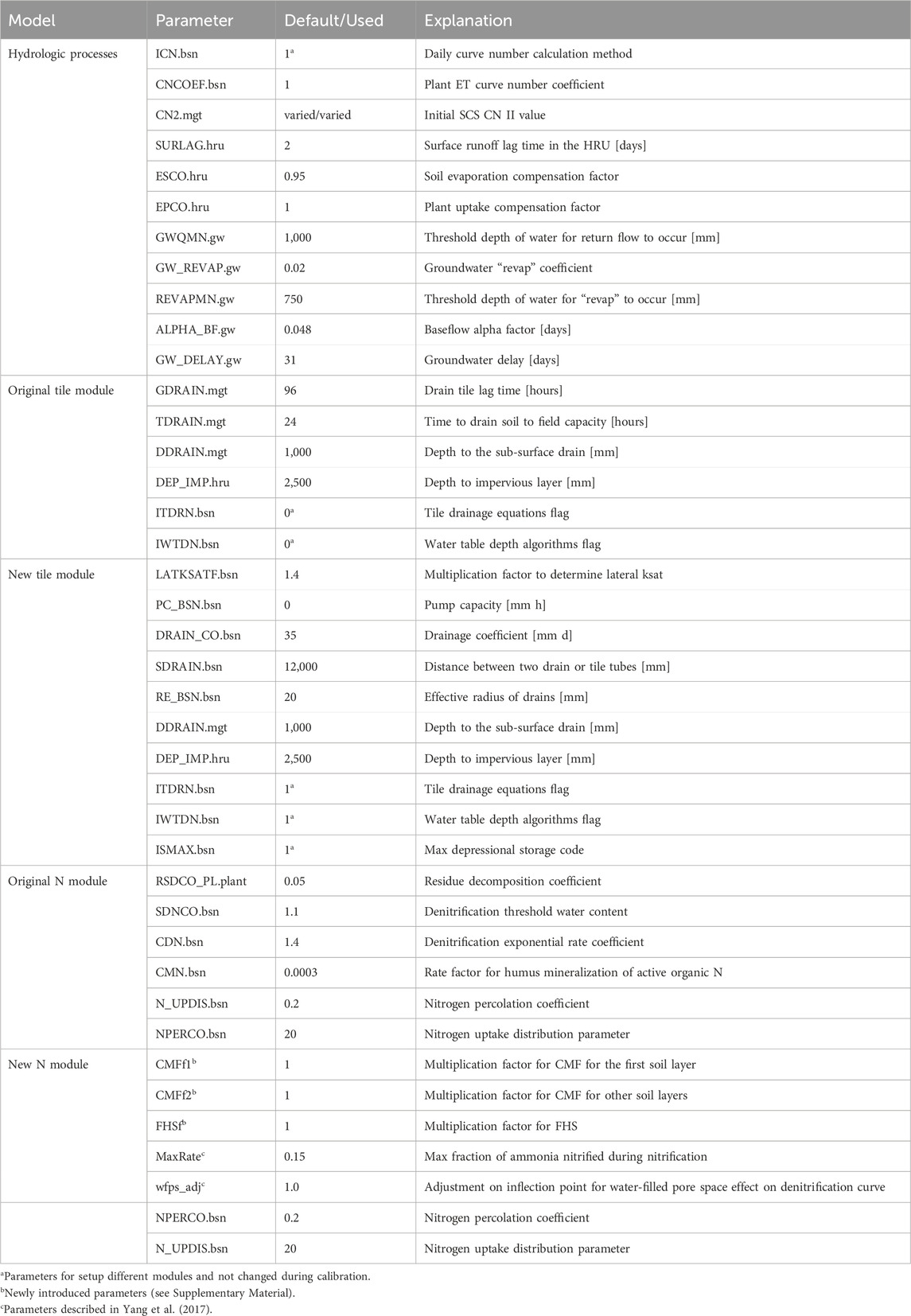
Table 1. Model parameters considered in model calibration.

2.2.2 Tile drainage modules

In SWAT, tile drainage can be calculated using two modules (Guo et al., 2018). The original tile drainage algorithm calculates tile flow as a function of water table depth, tile depth, and the time required to drain the soil to field capacity, assuming that the tile systems have equidistant tile spacing and size (Table 1) (Arnold et al., 1999; Du et al., 2005; Green et al., 2006). The new tile drainage algorithm computes tile flow using Hooghoudt’s steady state and Kirkham (van Schilfgaarde et al., 1957) tile drain equations that are a function of water table depth, tile drain depth, size, and spacing (Table 1), which are also used in the widely used DRAINMOD model (Skaggs et al., 2012). Previous studies incorporated and tested these equations within SWAT (Moriasi D. et al., 2007; Moriasi et al., 2012). These two methods were integrated with the “tip-bucket” soil water movement algorithm to simulate soil water balance for the drainage-based soil systems. Both methods for calculating tile drainage have been thoroughly tested against field and watershed scale drainage observations (Green et al., 2006; Moriasi et al., 2013b). Few studies have successfully simulated NO₃ ⁻ losses through tile drainage using the SWAT model (Schilling and Wolter, 2009; Moriasi et al., 2013a; Moriasi et al., 2013b; Gassman et al., 2014; Ikenberry et al., 2017).

2.3 Model setup, calibration, sensitivity and uncertainty analysis

Using a 10 m grid Digital Elevation Model (DEM), the SFW was divided into 115 subbasins, which were further segmented into 385 hydrologic response units (HRUs) based on the SSURGO database, a field-level land use map, and two slope categories (0%–2% and >2%). Typical management schedules for corn–soybean rotations were derived from the referenced cropland management dataset (Tomer et al., 2008a) and supplemented with estimates from Iowa State University Extension and Outreach. For instance, before the corn year, 75% of the total annual manure application was applied in the fall, while the remaining 25% was applied in the spring of the corn year (Supplementary Table S2). The model utilized NLDAS2 weather data for its inputs (Xia et al., 2012; Qi et al., 2019c). The presence of subsurface drains was assumed for all areas with hydric soils, with adjacent land also included due to the practice of draining a field if any of its interior area has poorly drained soils (Bailey et al., 2022). Therefore, an HRU was designated as a drain if it is covered by hydric soil (Figure 2d). The Penman-Monteith method was employed to estimate potential evapotranspiration, while the variable storage routing method was used for in-stream routing. Annual average wet and dry N deposition input was derived from the Clean Air Status and Trends Network (CASTNET).

The observed daily streamflow and NO₃ ⁻ load were evenly divided into calibration and validation periods (Supplementary Table S3). Before the calibration period, we used a 1-year (2000) warm-up period to initialize the model. Selected parameters for model calibration are shown in Table 1. We considered previous studies in the same watershed when selecting hydrologic, tile drainage, and soil N cycling parameters (Green et al., 2006; Moriasi et al., 2012; Moriasi et al., 2013b; Yang et al., 2017; Bailey et al., 2022). We employed a multi-station procedure to calibrate the streamflow and NO₃ ⁻ loads. The first step was to calibrate the streamflow of three stations, which is the key for the following water quality calibration. Following discharge calibration, the NO₃ ⁻ load of three stations was calibrated (Figure 4).

Figure 4

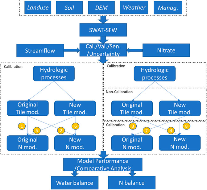
Figure 4. Flowchart of the study design, including SWAT setup; calibration and validation; sensitivity and uncertainty analyses; and the eight modeling configurations. The yellow circles represent the scenario numbers (Tables 2–5).

The Sequential Uncertainty Fitting algorithm version 2 (SUFI-2) method in SWAT-CUP (Abbaspour K. et al., 2007) was used to conduct calibration for daily flow rate and NO₃ ⁻ loads. It was also used to conduct parameter sensitivity and uncertainty analysis. Model performance was assessed according to percent bias (Pbias; Equation 1), coefficient of determination (R²; Equation 2), and Kling-Gupta efficiencies (KGE; Equation 3) (Knoben et al., 2019), given as:

$Pbias=100\times \frac{{\displaystyle {\sum }_{i=1}^N}\left(P_i-O_i\right)}{{\displaystyle {\sum }_{i=1}^N}{O}_i}(1)$

$R^2={\left(\frac{{\sum }_{i=1}^n\left(O_{i-}{O}_{avg}\right)·\left(P_i-P_{avg}\right)}{{\left[{\displaystyle {\sum }_{i=1}^n}{\left(O_{i-}{O}_{avg}\right)}^2·{\displaystyle {\sum }_{i=1}^n}{\left(P_i-P_{avg}\right)}^2\right]}^{0.5}}\right)}^2(2)$

$KGE=1-\sqrt{{\left(r-1\right)}^2+{\left(\alpha -1\right)}^2+{\left(\beta -1\right)}^2}(3)$

where $O_i$ and $P_i$ are the observed and modeled data, $O_{avg}$ and $P_{avg}$ their averages, $r$ the linear correlation between observed and modeled data, $\alpha$ the flow variability error, and $\beta$ bias term. Model performance criteria were established based on the guidelines provided by Moriasi DN. et al. (2007), operating under the assumption that the evaluation criteria for Nash-Sutcliffe Efficiency (NSE) are also applicable to R ² and KGE. KGE provides a more comprehensive assessment of model performance by evaluating not only the correlation between observed and simulated values but also accounting for the variability and bias in the simulations. Unlike NSE, which can be overly sensitive to outliers and can yield misleading results if the mean observed value is low, KGE incorporates multiple aspects of model performance. This makes KGE a more robust metric, particularly in complex hydrological systems where various factors can influence model outputs. The KGE was used as the objective function for calibrating daily streamflow and NO₃ ⁻ load, incorporating data from three monitoring stations with equal weighting in the function.

Parameter sensitivities were determined using the following multiple regression equation, based on results running the SUFI-2 procedure of SWAT-CUP multiple times, given as (Equation 4):

$\mathrm{g}=\mathrm{\alpha }+{\displaystyle \sum _{i=1}^m}{\beta }_i·b_i(4)$

where g is the objective function value, α and β _i are regression coefficients, b _i is the calibration parameter, and m is the number of parameters considered. KGE was used as the objective function value. The Student’s t-test was used to quantify the statistical significance of each parameter, with a p-value <0.05 indicating a parameter as sensitive in the present study. The global sensitivity analysis approach estimates the change in the objective function resulting from changes in each parameter while all other parameters are changing (Abbaspour K. et al., 2007), and as a result, it does not provide an absolute measure of the sensitivity but rather the relative sensitivity.

Prediction uncertainty was estimated through the SUFI-2 procedure (Abbaspour K. et al., 2007). In SUFI-2, the uncertainties in model structure, parameters, and input data are not separately estimated but are attributed as total model uncertainty to the parameters (Abbaspour K. et al., 2007). The Latin hypercube sampling method is used in SUFI-2 for vast parameter value combinations, and resultant model simulations are used to calculate the percentage of measured data bracketed by the 95 Percent Prediction Uncertainty (often referred to as 95PPU), which is measured by the p-factor. The range of the p-factor varies from 0.0 to 1.0, with values close to 1.0 (all observations bracketed by the prediction uncertainty) indicating very strong model performance and small prediction uncertainty. The r-factor is the average thickness of the 95PPU bands divided by the standard deviation of the observed data. The r-factor varying between 0 and 1.0 indicates acceptable prediction uncertainty estimation (Abbaspour K. et al., 2007; Abbaspour, 2013). In general, a trade-off between p-factor and r-factor exists for model uncertainty evaluation. A larger p-factor can be achieved at the expense of a larger r-factor, and vice versa. A model with a balance between the two factors can provide acceptable prediction uncertainty (Qi et al., 2019b).

2.4 Comparison of model configurations

We considered eight model configurations, which included: original and new tile drainage modules × calibration and non-calibration of tile drainage modules × original N module and new N module. Figure 4 illustrates the design of the eight model configurations and the step-wise calibration procedure. Here, we aimed to evaluate model performance under scenarios with calibrated and non-calibrated tile drainage parameters (Table 1), reflecting practical conditions where tile parameters may or may not be accurately known (Green et al., 2006; Moriasi et al., 2012; Schilling et al., 2019). For each of the eight model configurations, we independently calibrated the same set of parameters (Table 1). We then analyzed the eight simulations for water and soil N balance at the watershed scale and discussed the results as compared with previous studies. We calculated the average, standard deviation (SD), and coefficient of variation (CV) for water and N balance components across eight modeling simulations. The CV is a useful statistic that measures the relative variability of model outputs by comparing the standard deviation to the mean. The CV can help identify which processes exhibit greater variability across different model configurations (Butts et al., 2004). By assessing the CV of different outputs, we can prioritize areas that may need further investigation or refinement in model structure and parameterization.

3 Results and discussions

3.1 Model performance evaluation

The performance evaluation metrics for daily streamflow and NO₃ ⁻ load across the eight model configurations at the three outlets are summarized in Tables 2 and 3. The best-fit parameters for the eight model configurations are presented in Supplementary Tables S4 and S5. For daily streamflow simulations, R ² values ranged from 0.40 to 0.68, and KGE values from 0.46 to 0.80 during the calibration period, with Pbias between −7.7% and 19.6% across all eight model configurations and three stations. During the validation period, R ² values ranged from 0.49 to 0.68, KGE values from 0.51 to 0.77, and Pbias ranged between −27.2% and −11.4%. Overall, the model satisfactorily predicted daily streamflow across all configurations, though it generally underestimated streamflow during the validation period. For daily NO₃ ⁻ load simulations, during the calibration period, R ² and KGE values ranged from 0.33 to 0.57 and 0.39 to 0.60, respectively, with Pbias between −52.7% and −14.3%. During validation, the performance decreased, with R ² values from 0.21 to 0.48, KGE values from 0.05 to 0.58, and Pbias values ranging between −45.4% and −7.6% across all configurations and stations (Table 3). All models consistently tended to underestimate daily NO₃ ⁻ loads. Nevertheless, the new N module typically delivered superior performance over the original N module in predicting daily NO₃ ⁻ loads, regardless of tile module configuration (Table 3).

Table 2

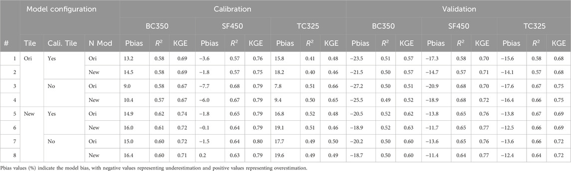
Table 2. Model performance evaluation for daily streamflow at three monitoring stations.

Table 3

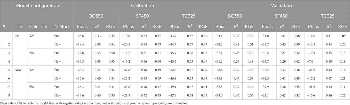
Table 3. Model performance evaluation for daily NO₃ ⁻ load at three monitoring stations.

We also evaluated daily and monthly simulations of streamflow and NO₃ ⁻ load for the combined calibration and validation periods (Supplementary Tables S6 and S7). Overall, daily streamflow showed R ² of 0.52–0.68, KGE of 0.63–0.79, and Pbias of −15% to −2%, while daily NO₃ ⁻ load had R ² of 0.32–0.47, KGE of 0.18–0.57, and Pbias of −30% to −12% across all configurations and stations. Monthly simulations generally yielded better model performance compared to daily simulations across all configurations and stations. For monthly streamflow, R ² and KGE values exceeded 0.69 and 0.79, respectively, with Pbias values ranging between −15% and −2%. Monthly NO₃ ⁻ load had R ² values ranging from 0.37 to 0.59, KGE values from 0.32 to 0.63, and Pbias from −30% to −14%. According to the performance criteria recommended by Moriasi DN. et al. (2007) for monthly simulations (assumed applicable for R ² and KGE), the majority of simulations achieved satisfactory results.

Overall, the new tile module improved daily and monthly streamflow simulations over the original, especially under the tile parameter calibration condition (Supplementary Tables S6 and S7). In addition, we did not observe a clear improvement in model performance when calibrating additional tile parameters for either the original or the new tile modules. In fact, in many cases, the original tile model without calibrated parameters provided better simulations of daily streamflow. This may be caused by the fact that adding more tile parameters to the hydrological parameter set increases model complexity, making it more difficult for auto-calibration to consistently capture the global optimum of the objective function (KGE in our case). It is recommended to maintain a balance between the number of parameters included and computational cost when using semi-distributed hydrological models such as SWAT (including more parameters does not necessarily lead to better results), and observed parameters should be utilized whenever possible.

Previous studies using SWAT to simulate daily streamflow highlighted persistent challenges in accurately capturing peak-flow events (Qi et al., 2019b; Kumar et al., 2024). Underestimation of streamflow during high-flow conditions directly contributes to the underestimation of NO₃ ⁻ loads (Qi et al., 2019a). Another critical reason for underestimating NO₃ ⁻ loads could be SWAT’s simplified representation of NO₃ ⁻ transport through tile drainage systems. Unlike the explicit numerical approach used by models such as DRAINMOD, which solves the advective-dispersive-reactive equation (Helwig et al., 2002), SWAT’s simplified coupling of soil water flow with NO₃ ⁻ leaching may require further refinement. Additionally, the model performance at the TC325 station for NO₃ ⁻ loads was consistently lower compared to the other two stations. This discrepancy is likely related to the significant presence of animal feeding operations, particularly swine production, within the Tipton Creek area (Tomer et al., 2008a; Tomer et al., 2008b). Due to insufficient information, the temporal and spatial patterns of manure application were not adequately represented in the model’s fertilization operations (Figure 2).

3.2 Model sensitivity and uncertainty analysis

We selected the most sensitive parameters affecting daily streamflow and NO₃ ⁻ load at the watershed outlets based on findings from previous studies for model calibration (Green et al., 2006; Moriasi et al., 2012; Moriasi et al., 2013a; Moriasi et al., 2013b). These parameters were then used for further sensitivity analysis, as summarized in Table 1. Sensitivity was assessed using p-values from Student’s t-tests, with the results presented in Supplementary Tables S8 and S9.

For daily streamflow, the most sensitive parameters in the original tile module without tile parameter calibration were primarily related to surface runoff and soil moisture (such as SURLAG, ESCO, EPCO, and CN2; see Table 1 for explanation; Supplementary Table S8). Although groundwater parameters were included in the calibration process, they did not show significant sensitivity to daily streamflow under this configuration. However, when tile parameters were calibrated, the most sensitive parameters shifted to include both groundwater (such as GWQMN, GW_REVAP, and REVAPMN) and tile drainage (such as DEP_IMP and GDRAIN) parameters (Tables 1; Supplementary Table S8). A similar pattern was observed in the new tile drainage module, suggesting that calibrating tile parameters increases the sensitivity of groundwater parameters to streamflow simulation. Despite these shifts in sensitivity, the overall model performance did not improve when tile parameters were calibrated compared to configurations without tile calibration (Table 2). This could be due to the relatively low contribution of groundwater discharge to streamflow compared to surface runoff and drainage flow in the SFW (Supplementary Table S12).

Regarding the daily NO₃ ⁻ load, the parameters found to be most sensitive for the original N module were primarily associated with denitrification processes (CDN) and mineralization processes (CMN) (Tables 1; Supplementary Table S9). In contrast, parameters controlling organic matter decomposition rates and the initial fraction of fresh humus (FHS)—notably CMFm2 and fFHS (Table 1; Supplementary Table S9)—showed high sensitivity for the new N module. Additionally, the parameter governing denitrification processes (i.e., wfps_adj) was also very sensitive (Table 3). Upon examination of the denitrification-related parameters (Supplementary Tables S4 and S5), we found that low values of wfps_adj were associated with increased denitrification rates for the new N module (A detailed discussion of this parameter is provided in the Supplementary Material).

Supplementary Tables S10 and S11 present the p-factor and r-factor values for the estimated 95PPU bands of daily streamflow and NO₃ ⁻ fluxes across the eight model configurations. The p-factor values showed that the 95PPU bands captured 27%–52% of observed daily streamflow and only 14%–34% of observed NO₃ ⁻ loads. The r-factor ranged from 0.32 to 0.59 for observed daily streamflow and from 0.26 to 0.60 for observed NO₃ ⁻ loads. Overall, the low p-factor values indicated a high level of uncertainty in the predictions of both daily streamflow and NO₃ ⁻ load across three monitoring stations. This overall decrease in p-factor from streamflow to NO₃ ⁻ load suggested that modeling uncertainty was greater for NO₃ ⁻ load than for streamflow simulation. This result was expected, as streamflow simulation was primarily influenced by hydrological processes, whereas NO₃ ⁻ simulation depended on both hydrological and biogeochemical processes. The added complexity of N cycling introduced greater challenges, contributing to the lower p-factor values observed for NO₃ ⁻ predictions compared to streamflow.

3.3 Water balance assessment across model configurations

Table 4 shows the annual water budget for the eight model configurations in the SFW. Average, SD, and CV were also calculated for the water budget across eight model configurations. The average annual precipitation in the watershed from 2001 to 2018 was 894 mm, while the average annual potential evapotranspiration (PET) was 1,137 mm. Actual evapotranspiration (ET) ranged from 586 to 613 mm, with an average of 597 mm, which represents about 67% of the average annual precipitation (Supplementary Table S12). The total water yield (= surface runoff + lateral flow + groundwater flow + drainage flow) accounted for approximately 34% of the average annual precipitation (Supplementary Table S12). Surface runoff varied between 44 and 110 mm, averaging 88 mm, which constitutes about 31% of the total water yield. Baseflow ranged from 48 to 63 mm, with an average of 55 mm, making up about 18% of the total water yield (Supplementary Table S12). Drainage flow ranged from 119 to 194 mm, averaging 154 mm, which accounts for approximately 50% of the total water yield (Supplementary Table S12). Lateral flow ranged from 3 to 14 mm, averaging 6 mm, making up about only 2% of the total water yield (Supplementary Table S12).

Table 4

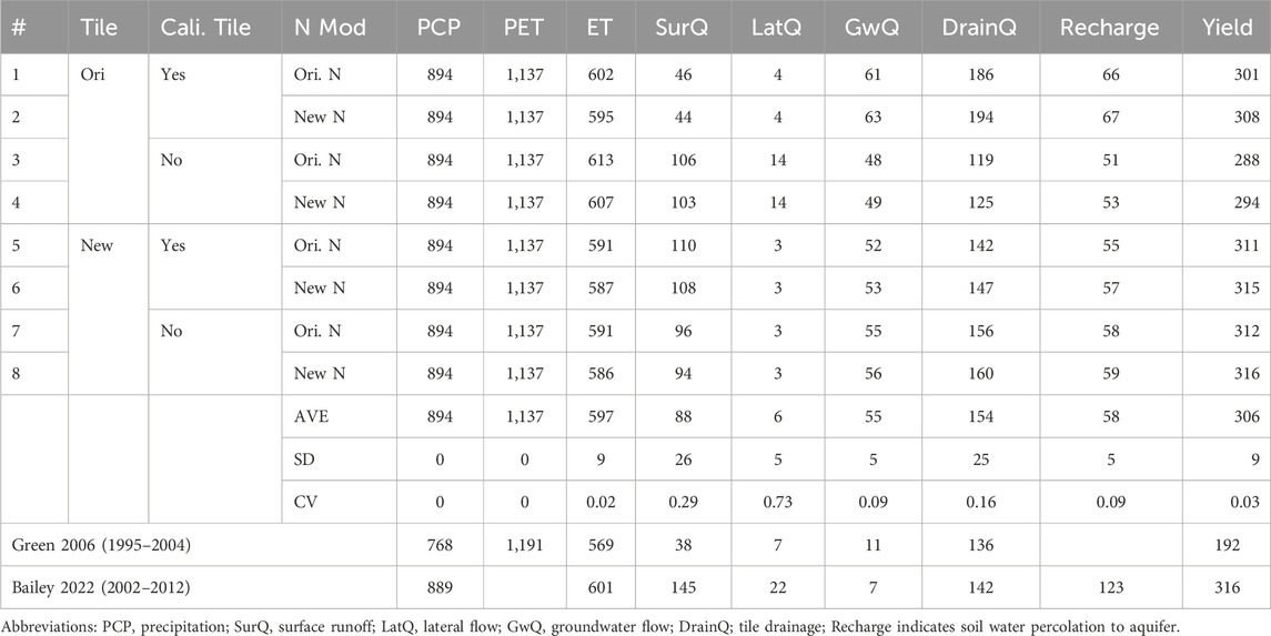
Table 4. Annual average water budgets (in mm H₂O) in the south fork of the iowa river watershed (SFW) for the eight model configurations over 2001–2018.

Lateral flow showed the highest coefficient of variation (CV = 0.7), although its magnitude was an order of magnitude lower than that of surface runoff and drainage flow. We also observed significantly greater variation between calibration and non-calibration model configurations for the original tile module compared to the new tile module for both surface runoff and drainage flow. When calibrated, the original tile module generated considerably less surface runoff and more drainage flow than in the non-calibrated condition, whereas the new tile drainage module showed similar results regardless of calibration. Interestingly, the non-calibrated original tile module produced results more comparable to the new tile module under both calibration and non-calibration conditions. These results suggest that obtaining consistent and reliable results necessitates more detailed information about actual field conditions, as relying solely on parameter calibration without accurate tile data may lead to a skewed water budget for tile drainage systems.

Table 4 also shows the comparison between previous studies and this study on water budget, and Supplementary Table S12 shows important hydrological component ratios at the SFW. It should be noted that the study area of Bailey et al. (2022), which used SF450 as the outlet, was smaller than the area considered in this study (Figure 2). This study had close annual precipitation of 894 mm to Bailey et al. (2022)(889 mm) both of which were higher than that of Green et al. (2006) (768 mm) due to different study periods. Accordingly, the ET values were also close between this study and that of Bailey et al. (2022) (601 mm) and greater than that of Green et al. (2006) (569 mm). Total water yield—comprising surface runoff, lateral flow, groundwater flow, and tile drainage flow—accounted for 32%–35% of annual precipitation. This figure surpassed the 25% reported by Green et al. (2006) but fell short of the 36% noted by Bailey et al. (2022). Surface runoff represented 5%–12% of annual precipitation, higher than the 5% documented by Green et al. (2006) but lower than the 16% observed by Bailey et al. (2022). A similar trend was seen in the contribution of surface runoff to total water yield, with our study accounting for 14%–37%, most of which were greater than the 20% cited by Green et al. (2006) and less than the 46% reported by Bailey et al. (2022).

Total subsurface flow, which includes lateral flow, groundwater flow, and tile drainage flow, accounted for 20%–29% of annual precipitation in this study, most of which were higher than the 20% reported by Green et al. (2006) and the 19% noted by Bailey et al. (2022). The increase was primarily due to the groundwater discharge simulated in this study, which constituted 17%–20% of total water yield, significantly higher than the 6% from Green et al. (2006) and 2% from Bailey et al. (2022). In contrast, the lateral flow represented only 1%–5% of total water yield, most of which was less than the 4% from Green et al. (2006) and 7% from Bailey et al. (2022). This made lateral flow the smallest contributor to total water yields in both this study and Green et al. (2006), whereas Bailey et al. (2022) identified groundwater flow as the least contributor. Our drainage flow accounted for 13%–22% of annual precipitation, which was close to the 16% reported by Bailey et al. (2022) and 18% estimated by Green et al. (2006). Moreover, drainage flow made up 41%–63% of total water yield, most of which exceeded the 45% from Bailey et al. (2022) but fell short of the 71% reported by Green et al. (2006). The fraction of drainage flow in total water yield aligns with the range of 46%–54% reported by Schilling et al. (2019) in their analytical and SWAT modeling of a similar drained watershed (Boon River watershed) in the Des Moines Lobe of north-central Iowa.

Overall, our results using both tile modules to analyze the water budget in the SFW were mostly consistent with the findings of the SWAT modeling study by Green et al. (2006) and the SWAT + MODFLOW modeling study by Bailey et al. (2022). Additionally, our findings aligned with the fieldwork conducted by Tomer et al. (2008b), demonstrating the robustness of the two tile modules in simulating hydrological processes within tile-drained agricultural ecosystems.

3.4 Nitrogen balance assessment across model configurations

Table 5 presents the average annual N budget for the entire SFW across eight model configurations for the period 2001–2018. Average, SD, and CV were also calculated for the N budget. The average annual N fertilization amounted to 90 kg N ha⁻¹ in mineral form and 55 kg N ha⁻¹ in organic form (Supplementary Table S2). Average annual atmospheric deposition of N was about 21 kg N ha⁻¹. Biological N fixation ranged from 42 to 79 kg N ha⁻¹, averaging 56 kg N ha⁻¹. Residue-derived organic N inputs to the soil ranged from 79 to 128 kg N ha⁻¹, averaging 103 kg N ha⁻¹. Net mineralization of organic matter produced 106–181 kg N ha⁻¹, averaging 154 kg N ha⁻¹. Plant uptake ranged from 164 to 278 kg N ha⁻¹, averaging 218 kg N ha⁻¹. Denitrification loss ranged from 13 to 33 kg N ha⁻¹, averaging 26 kg N ha⁻¹, while volatilization (NH₃) ranged from 1 to 3 kg N ha⁻¹, averaging 2 kg N ha⁻¹. The NO₃ ⁻ loss via drainage flow ranged from 22 to 30 kg N ha⁻¹, averaging 25 kg N ha⁻¹, and leaching NO₃ ⁻ ranged from 8 to 10 kg N ha⁻¹, averaging 9 kg N ha⁻¹. The NO₃ ⁻ loss via surface runoff, lateral flow, and groundwater averaged 2, 1, and 0.3 kg N ha⁻¹ across eight model configurations (Table 5). Organic N losses via surface runoff ranged from 1 to 20 kg N ha⁻¹ with a high CV of 0.9. Organic N removed through crop harvest ranged from 131 to 150 kg N ha⁻¹. N₂O fluxes ranged from 6 to 12 kg N ha⁻¹, NO fluxes from 5 to 7 kg N ha⁻¹, and N₂ fluxes from 6 to 11 kg N ha⁻¹. In addition, we calculated changes in mineral N and total N in the soil profile, which ranged from −60 to 21 kg N ha⁻¹ (with a high |CV| = 1.4) and from −6–37 kg N ha⁻¹ (with a high CV of 1.8), respectively.

Table 5

Table 5. Annual nitrogen budgets (kg N ha⁻¹) for the entire south fork of the iowa river watershed (SFW) under eight model configurations (2001–2018); values in brackets represent nitrification gas fluxes.

Since no prior studies on N balance have been conducted in the SFW, we compared our results with those from research performed at the nearby Kelley experimental site (Figure 1) (Li et al., 2008; Gillette et al., 2018). Two ecosystem modeling efforts have been undertaken at the Kelley site over different periods to assess the effects of cover crops on NO₃ ⁻ loss through tile drainage and N₂O fluxes. For our analysis, we chose results from the control scenario that did not include cover crops, as the majority of agricultural land in the SFW does not utilize cover crops. Table 5 presents a comparison between the previous studies at the Kelley site and our findings regarding N budgets, and Supplementary Table S13 also lists key component ratios. It is noted that we assumed identical atmospheric deposition for both sites, and the two previous studies did not report all balance components.

At the SFW, the annual N uptake comprised 65%–97% of the total mineral N input, which includes mineral fertilization, atmospheric deposition, and net mineralization. Denitrification accounted for approximately 7%–13% of the total input, while N₂O contributed about 2%–4%. Drainage losses were 8%–12% of total input. Compared to the Kelley site, the SFW had higher N fertilization, resulting in higher net mineralization than at the Kelley site. Nitrogen fixation at the SFW site was lower, likely due to higher overall nitrogen application rates compared to the Kelley site. Another possible reason for the underestimation of N fixation could be inadequate calibration of crop growth processes. Additional observations of crop yield and/or biomass would help improve the simulation of crop growth–induced N dynamics. The N uptake to total mineral N input ratio in the SFW was less than the 1.1 reported by Gillette et al. (2018) and the 1.21 from Li et al. (2008) at the Kelley site, indicating less N use efficiency in the SFW. Additionally, denitrification was higher in the SFW—particularly when using the original N module—compared with the Kelley site, with denitrification ratios over total input at 0.07–0.13 for this study compared to 0.07 for Gillette et al. (2018) and 0.03 for Li et al. (2008). Simulated total N₂O fluxes were also greater in the SFW than in the Kelley site, although the N₂O to input ratio was similar (0.02–0.04). In contrast, NO₃ ⁻ loss via drainage flow was lower in the SFW than at the Kelley site, with a drainage N loss to input ratio of 0.08–0.12, which is less than the ratios of 0.17 from Li et al. (2008) and 0.19 from Gillette et al. (2018).

Simulated denitrification in the new N module was consistently lower than in the original module across all tile configurations (13–27 vs 29–33, respectively). As a result, the original module estimated denitrification rates that exceeded simulated drainage NO₃ ⁻ losses, while the new module produced estimates below those losses (Table 5). Although denitrification rates could not be validated in SFW due to a lack of observations, the results from the new N module aligned more closely with those from the Kelley site, suggesting improved denitrification simulation. In addition, denitrification simulated by the new N module was more sensitive to soil moisture than in the original module, as reflected in the differences among tile drainage modules and their calibration approaches. For example, the new N module showed substantial discrepancies in denitrification between calibrated and non-calibrated configurations (24 vs 13 kg N ha⁻¹ with the original tile module; 27 vs 19 kg N ha⁻¹ with the new tile module), whereas the original N module produced more consistent results (29 and 33 kg N ha⁻¹ with the new and original tile modules, respectively).

Most N gas fluxes originated from denitrification and were near the upper range of literature-reported values, particularly for NO and N₂O (Bouwman et al., 2002; Hoben et al., 2011; Castellano et al., 2012; Butterbach-Bahl et al., 2013; Castellano et al., 2019; Ma et al., 2022). And most of the N₂O results were also greater than that reported in Gillette et al. (2018). Although the new N module improved denitrification simulation, an accurate representation of N gas fluxes still requires additional field measurements. In particular, the NO: N₂O: N₂ ratios are strongly influenced by soil moisture dynamics (Potter et al., 1996; Parton et al., 2001), emphasizing the importance of complementary observations (e.g., soil moisture and routinely measured N₂O fluxes) to better constrain model parameters and improve watershed-scale N budget assessments. For instance, the DayCent model represents the topsoil with finer vertical resolution (typically 2 cm for the first layer and 3 cm for the second) compared to SWAT, which uses a fixed 1 cm first layer and approximately 20 cm for the second. This coarser layering in SWAT necessitates careful calibration against observed soil moisture, which strongly influences N gas fluxes.

Furthermore, we found that the new N module simulated substantially lower organic N losses via surface runoff compared to the original N module (1 vs 10–20 kg N ha⁻¹), regardless of the tile module configuration (Table 5). This result indicates that, according to the new N module, residue and soil organic matter in the surface layer decomposed more rapidly than simulated by the original N module. One potential solution to the underestimation of organic N loss via surface runoff is to incorporate a passive humus pool, which is currently not represented for the surface soil layer (Zhang et al., 2013). Additionally, the large variability in soil mineral N and total soil N changes across the eight model configurations underscores the substantial uncertainty in soil N cycling processes. The general positive changes in soil N (Table 5) suggest that the system may have been accumulating N, potentially contributing to legacy N. Since the current SWAT model cannot simulate legacy N storage and release, this limitation may partly explain the underestimation of NO₃ ⁻ loads at the outlets. It is worth noting that the SFW produced an excessive NO₃ ⁻ load, with an average NO₃ ⁻ yield of ∼38 kg N ha⁻¹ yr⁻¹ at station SF450 for 2001–2018 (See the comparison with USGS estimations in Supplementary Figure S2), whereas multiyear average NO₃ ⁻ yields in Iowa typically range from 15 to 30 kg N ha⁻¹ yr⁻¹ (Jones et al., 2018a; Jones et al., 2018b).

In contrast to the large variations in simulated denitrification and associated N gas fluxes, we found that drainage NO₃ ⁻ losses were much more consistent across different model configurations. In addition, all models tended to simulate relatively low volatilization. Although few studies have reported volatilization results using SWAT, our findings highlight the need to improve its representation in the model (Lian et al., 2021). Compared to the original N module, the new N module was more sensitive to environmental changes. This requires careful monitoring of changes in organic C and N, as well as decomposition and mineralization rates. The original N module has the advantage of providing relatively stable and reasonable N cycling simulations without needing to account for C processes in detail. In contrast, the new N module necessitates careful calibration of initial humus pool partitioning, as it relies on these pools for accurate simulations (see sensitivity analysis).

3.5 Limitation and future research

While the simulation results for streamflow were robust, the accuracy of NO₃ ⁻ load simulations was comparatively lower. It is widely recognized that SWAT and other hydrological models generally perform better in simulating hydrological processes than in nutrient cycling. In this study, one contributing factor to the reduced performance in simulating NO₃ ⁻ was the insufficient representation of NO₃ ⁻ leaching processes, especially as affected by tile drainage. Improving this aspect may necessitate further development of a more physically-based model to enhance future outcomes. In addition, the interaction of tile drainage with streamflow is more intricate than what the current model configuration can capture. Features such as potholes or depressions that receive inflow can be considered in the modeling, but the added complexity of these landscape hydrological pathways may reduce overall model performance and complicate the calibration process (Du et al., 2005; Beeson et al., 2011; Beeson et al., 2014). Another reason for the underestimation of NO₃ ⁻ load is the lack of accurate input data, such as the quantity and timing of mineral fertilizer and manure applications, as well as detailed crop management practices, all of which strongly influence soil N dynamics (Ren et al., 2022; Niroula et al., 2023).

This study illustrates a common challenge encountered in the application of the SWAT model, where only discharge and water quality data are available from limited subbasin outlets. The calibration of soil water and nutrient parameters using water quantity and quality data with the original soil N module is widely used within the SWAT community. However, when more complex hydrological and biogeochemical processes, such as tile drainage and N gas fluxes, are incorporated into the model, relying solely on outlet water data to calibrate soil process parameters can lead to significant uncertainty in predictions (Arnold et al., 2015). The new N module adopts the Century/DayCent model approach to simulate N gas fluxes, including N₂O, NO, and N₂, originating from nitrification and denitrification (Figure 3). To effectively use the more complex model and reduce prediction uncertainty, additional observations—such as soil moisture and the commonly measured N₂O flux—is needed (Del Grosso et al., 2020). Although SWAT employs a simplified “tipping-bucket” soil water module, it can provide reasonable estimates of soil water dynamics when calibrated with soil moisture data (Qi et al., 2018). In addition, except for requiring additional field observations, it is important to simulate nutrient dynamics within a watershed—not just loads at the outlet—using soft data (Arnold et al., 2015). Proper process representation supported by soft data can significantly improve model calibration and validation. Soft data sources may include peer-reviewed literature, technical reports, theses, and field surveys.

4 Conclusion

This study used a comparative modeling framework to evaluate SWAT’s ability to simulate watershed-scale tile drainage and N losses (NO₃ ⁻ leaching and N-gas fluxes) in a representative Midwestern tile-drained watershed. Eight configurations were tested by pairing original vs. new tile-drainage modules, calibrated vs. default tile parameters, and original vs. new N modules. Daily streamflow and NO₃ ⁻ loads from three monitoring stations (two: 2001–2018; one: 2001–2010) supported calibration, validation, sensitivity, and uncertainty analyses, and watershed-scale water and N balances were compared with prior work, including the nearby Kelley experimental site.

Model evaluation indicated that all eight model configurations effectively simulated daily and monthly streamflow and NO₃ ⁻ loads, though they tended to underestimate peak streamflow and NO₃ ⁻ loads. The watershed-scale water balance terms mostly fell within the range reported in previous studies. We found that the new tile module generally enhanced daily streamflow predictions compared to the original module, particularly under the conditions of calibrated tile parameters. For both the new and original tile modules, further calibration of additional tile parameters did not lead to noticeable improvements in daily streamflow. Meanwhile, the new N module consistently outperformed the original N module in simulating daily and monthly NO₃ ⁻ loads, regardless of the tile module configuration used. Parameter sensitivity and uncertainty analyses revealed high uncertainty, particularly for NO₃ ⁻ load predictions at all three monitoring stations due to the complexity of N cycling processes. Specifically, we found that denitrification and associated N gas fluxes (inducing N₂O, NO, and N₂) varied across configurations, reflecting fundamental differences between the original and new N modules. The N budget also deviated from values reported at the Kelley site, indicating that relying solely on outlet NO₃ ⁻ load data is insufficient to capture key soil N cycling processes.

The new tile module is preferable for streamflow simulation, and the new N module strengthens NO₃ ⁻ load predictions; however, the expanded process representation for N gases amplifies uncertainty when calibration data are sparse. To reduce uncertainty in denitrification and N-gas estimates, multi-constraint calibration is recommended—pair outlet NO₃ ⁻ loads with supplemental observations (e.g., soil moisture and N₂O fluxes) and/or soft data. The comparative approach proved effective for identifying process controls and data gaps, guiding targeted monitoring to improve SWAT performance in tile-drained watersheds. In sum, the comparative evaluation clarifies where SWAT performs robustly (streamflow, NO₃ ⁻ loads) and where additional observations are essential (N-gas fluxes), providing actionable direction for future model development, calibration strategies, and data collection in tile-drained systems.

Data availability statement

The raw data supporting the conclusions of this article will be made available by the authors, without undue reservation.

Author contributions

JQ: Project administration, Funding acquisition, Formal Analysis, Software, Writing – review and editing, Conceptualization, Methodology, Writing – original draft. RM: Writing – review and editing, Resources, Data curation, Investigation, Validation. KL: Data curation, Methodology, Investigation, Resources, Writing – review and editing. KC: Writing – review and editing, Resources, Data curation. BE: Resources, Validation, Writing – review and editing, Data curation, Investigation. DM: Data curation, Investigation, Writing – review and editing, Supervision. MS: Writing – review and editing, Data curation, Resources. MC: Writing – review and editing, Resources, Data curation.

Funding

The author(s) declare that financial support was received for the research and/or publication of this article. The funding support for this study was provided by the U.S. Department of Agriculture, the National Institute of Food and Agriculture (2021-67019-33684 and 2023-67019-39221). This research was a contribution from the Long-Term Agroecosystem Research (LTAR) network. LTAR is supported by the United States Department of Agriculture. The USDA is an equal opportunity provider and employer.

Conflict of interest

The authors declare that the research was conducted in the absence of any commercial or financial relationships that could be construed as a potential conflict of interest.

Generative AI statement

The author(s) declare that no Generative AI was used in the creation of this manuscript.

Any alternative text (alt text) provided alongside figures in this article has been generated by Frontiers with the support of artificial intelligence and reasonable efforts have been made to ensure accuracy, including review by the authors wherever possible. If you identify any issues, please contact us.

Publisher’s note

All claims expressed in this article are solely those of the authors and do not necessarily represent those of their affiliated organizations, or those of the publisher, the editors and the reviewers. Any product that may be evaluated in this article, or claim that may be made by its manufacturer, is not guaranteed or endorsed by the publisher.

Supplementary material

The Supplementary Material for this article can be found online at: https://www.frontiersin.org/articles/10.3389/fenvs.2025.1651136/full#supplementary-material

References

Abbaspour, K. C. (2013). SWAT-CUP 2012: SWAT calibration and uncertainty programs–a user manual. Dübendorf, Switzerland: Eawag, 103.

Google Scholar

Abbaspour, K. C., Vejdani, M., Haghighat, S., and Yang, J. (2007a). “SWAT-CUP calibration and uncertainty programs for SWAT,” in MODSIM 2007 international congress on modelling and simulation, modelling and simulation society of Australia and New Zealand. Dübendorf, Switzerland: Swiss Federal Institute of Aquatic Science and Technology, 1596–1602.

Google Scholar

Abbaspour, K. C., Yang, J., Maximov, I., Siber, R., Bogner, K., Mieleitner, J., et al. (2007b). Modelling hydrology and water quality in the pre-alpine/alpine Thur watershed using SWAT. J. Hydrol. 333 (2-4), 413–430. doi:10.1016/j.jhydrol.2006.09.014

CrossRef Full Text | Google Scholar

Arnold, J. G., Srinivasan, R., Muttiah, R. S., and Williams, J. R. (1998). Large area hydrologic modeling and assessment part I: model development. JAWRA J. Am. Water Resour. Assoc. 34 (1), 73–89. doi:10.1111/j.1752-1688.1998.tb05961.x

CrossRef Full Text | Google Scholar

Arnold, J., Gassman, P., King, K., Saleh, A., and Sunday, U. (1999). Validation of the subsurface tile flow component in the SWAT model. Trans. ASAE, 99–2138.

Google Scholar

Arnold, J. G., Youssef, M. A., Yen, H., White, M. J., Sheshukov, A. Y., Sadeghi, A. M., et al. (2015). Hydrological processes and model representation: impact of soft data on calibration. Trans. ASABE 58 (6), 1637–1660. doi:10.13031/trans.58.10726

CrossRef Full Text | Google Scholar

Awale, R., Chatterjee, A., Kandel, H., and Ransom, J. K. (2015). Tile drainage and nitrogen fertilizer management influences on nitrogen availability, losses, and crop yields. Open J. Soil Sci. 5 (10), 211–226. doi:10.4236/ojss.2015.510021

CrossRef Full Text | Google Scholar

Bailey, R. T., Bieger, K., Flores, L., and Tomer, M. (2022). Evaluating the contribution of subsurface drainage to watershed water yield using SWAT+ with groundwater modeling. Sci. Total Environ. 802, 149962. doi:10.1016/j.scitotenv.2021.149962

PubMed Abstract | CrossRef Full Text | Google Scholar

Baker, J., and Johnson, H. (1977). Impact of subsurface drainage on water quality. Proceedings, third national drainage symposium, Chicago, United States, December 1976, 91–298.

Google Scholar

Beeson, P., Doraiswamy, P., Sadeghi, A., Di Luzio, M., Tomer, M., Arnold, J., et al. (2011). Treatments of precipitation inputs to hydrologic models. Trans. ASABE 54 (6), 2011–2020. doi:10.13031/2013.40652

CrossRef Full Text | Google Scholar

Beeson, P. C., Sadeghi, A. M., Lang, M. W., Tomer, M. D., and Daughtry, C. S. (2014). Sediment delivery estimates in water quality models altered by resolution and source of topographic data. J. Environ. Qual. 43 (1), 26–36. doi:10.2134/jeq2012.0148

PubMed Abstract | CrossRef Full Text | Google Scholar

Bouwman, A., Boumans, L., and Batjes, N. (2002). Emissions of N₂O and NO from fertilized fields: summary of available measurement data. Glob. Biogeochem. Cycles 16 (4), 6-1-6–13. doi:10.1029/2001gb001811

CrossRef Full Text | Google Scholar

Burton, D. L., Wilts, H., and Macleod, J. (2024). Dissolved nitrous oxide emissions associated with agricultural drainage water as influenced by manure application. Front. Environ. Sci. 12, 1479754. doi:10.3389/fenvs.2024.1479754

CrossRef Full Text | Google Scholar

Butterbach-Bahl, K., Baggs, E. M., Dannenmann, M., Kiese, R., and Zechmeister-Boltenstern, S. (2013). Nitrous oxide emissions from soils: how well do we understand the processes and their controls? Philosophical Trans. R. Soc. B Biol. Sci. 368 (1621), 20130122. doi:10.1098/rstb.2013.0122

PubMed Abstract | CrossRef Full Text | Google Scholar

Butts, M. B., Payne, J. T., Kristensen, M., and Madsen, H. (2004). An evaluation of the impact of model structure on hydrological modelling uncertainty for streamflow simulation. J. Hydrol. 298 (1-4), 242–266. doi:10.1016/j.jhydrol.2004.03.042

CrossRef Full Text | Google Scholar

Castellano, M., Helmers, M., Sawyer, J., Christianson, L., and Barker, D. (2012). Nitrogen, carbon, and phosphorus balances in Iowa cropping systems: sustaining the soil resource. 2012 Integrated crop management conference - Iowa State University.

Google Scholar

Castellano, M. J., Archontoulis, S. V., Helmers, M. J., Poffenbarger, H. J., and Six, J. (2019). Sustainable intensification of agricultural drainage. Nat. Sustain. 2 (10), 914–921. doi:10.1038/s41893-019-0393-0

CrossRef Full Text | Google Scholar

Chen, R., Shen, W., Chen, Z., Guo, J., Yang, L., Fei, G., et al. (2024). Modulation of soil nitrous oxide emissions and nitrogen leaching by hillslope hydrological processes. Sci. Total Environ. 951, 175637. doi:10.1016/j.scitotenv.2024.175637

PubMed Abstract | CrossRef Full Text | Google Scholar

Crossman, J., Futter, M., Whitehead, P. G., Stainsby, E., Baulch, H., Jin, L., et al. (2014). Flow pathways and nutrient transport mechanisms drive hydrochemical sensitivity to climate change across catchments with different geology and topography. Hydrology Earth Syst. Sci. 18 (12), 5125–5148. doi:10.5194/hess-18-5125-2014

CrossRef Full Text | Google Scholar

Del Grosso, S., Parton, W., Mosier, A., Ojima, D., Kulmala, A., and Phongpan, S. (2000). General model for N₂O and N₂ gas emissions from soils due to dentrification. Glob. Biogeochem. Cycles 14 (4), 1045–1060. doi:10.1029/1999gb001225

CrossRef Full Text | Google Scholar

Del Grosso, S. J., Smith, W., Kraus, D., Massad, R. S., Vogeler, I., and Fuchs, K. (2020). Approaches and concepts of modelling denitrification: increased process understanding using observational data can reduce uncertainties. Curr. Opin. Environ. Sustain. 47, 37–45. doi:10.1016/j.cosust.2020.07.003

CrossRef Full Text | Google Scholar

Dinnes, D. L., Karlen, D. L., Jaynes, D. B., Kaspar, T. C., Hatfield, J. L., Colvin, T. S., et al. (2002). Nitrogen management strategies to reduce nitrate leaching in tile-drained midwestern soils. Agron. J. 94 (1), 153–171. doi:10.2134/agronj2002.1530

CrossRef Full Text | Google Scholar

Du, B., Arnold, J., Saleh, A., and Jaynes, D. (2005). Development and application of SWAT to landscapes with tiles and potholes. Trans. ASAE 48 (3), 1121–1133. doi:10.13031/2013.18522

CrossRef Full Text | Google Scholar

Du, B., Saleh, A., Jaynes, D., and Arnold, J. (2006). Evaluation of SWAT in simulating nitrate nitrogen and atrazine fates in a watershed with tiles and potholes. Trans. ASABE 49 (4), 949–959. doi:10.13031/2013.21746

CrossRef Full Text | Google Scholar

Fabrizzi, K. P., Fernández, F., G., Venterea, R. T., and Naeve, S. L. (2024). Nitrous oxide emissions from soybean in response to drained and undrained soils and previous corn nitrogen management. 53 (4), 407–417.

CrossRef Full Text | Google Scholar

Ford, W. I., King, K., and Williams, M. R. (2018). Upland and in-stream controls on baseflow nutrient dynamics in tile-drained agroecosystem watersheds. J. Hydrol. 556, 800–812. doi:10.1016/j.jhydrol.2017.12.009

CrossRef Full Text | Google Scholar

Gassman, P. W., Sadeghi, A. M., and Srinivasan, R. (2014). Applications of the SWAT model special section: overview and insights. J. Environ. Qual. 43 (1), 1–8. doi:10.2134/jeq2013.11.0466

PubMed Abstract | CrossRef Full Text | Google Scholar

Ghimire, U., Shrestha, N. K., Biswas, A., Wagner-Riddle, C., Yang, W., Prasher, S., et al. (2020). A review of ongoing advancements in soil and water assessment tool (SWAT) for nitrous oxide (N₂O) modeling. Atmosphere 11 (5), 450. doi:10.3390/atmos11050450

CrossRef Full Text | Google Scholar

Gillette, K., Malone, R., Kaspar, T., Ma, L., Parkin, T., Jaynes, D., et al. (2018). N loss to drain flow and N₂O emissions from a corn-soybean rotation with winter rye. Sci. Total Environ. 618, 982–997. doi:10.1016/j.scitotenv.2017.09.054

PubMed Abstract | CrossRef Full Text | Google Scholar

Green, C., Tomer, M., Di Luzio, M., and Arnold, J. (2006). Hydrologic evaluation of the soil and water assessment tool for a large tile-drained watershed in Iowa. Trans. ASABE 49 (2), 413–422. doi:10.13031/2013.20415

CrossRef Full Text | Google Scholar

Groffman, P. M., Butterbach-Bahl, K., Fulweiler, R. W., Gold, A. J., Morse, J. L., Stander, E. K., et al. (2009). Challenges to incorporating spatially and temporally explicit phenomena (hotspots and hot moments) in denitrification models. Biogeochemistry 93, 49–77. doi:10.1007/s10533-008-9277-5

CrossRef Full Text | Google Scholar

Gu, J., Nicoullaud, B., Rochette, P., Grossel, A., Hénault, C., Cellier, P., et al. (2013). A regional experiment suggests that soil texture is a major control of N₂O emissions from tile-drained winter wheat fields during the fertilization period. Soil Biol. Biochem. 60, 134–141. doi:10.1016/j.soilbio.2013.01.029

CrossRef Full Text | Google Scholar

Guo, T., Gitau, M., Merwade, V., Arnold, J., Srinivasan, R., Hirschi, M., et al. (2018). Comparison of performance of tile drainage routines in SWAT 2009 and 2012 in an extensively tile-drained watershed in the Midwest. Hydrology Earth Syst. Sci. 22 (1), 89–110. doi:10.5194/hess-22-89-2018

CrossRef Full Text | Google Scholar

Hama-Aziz, Z. Q., Hiscock, K. M., and Cooper, R. J. (2017). Dissolved nitrous oxide (N₂O) dynamics in agricultural field drains and headwater streams in an intensive arable catchment. Hydrol. Process. 31 (6), 1371–1381. doi:10.1002/hyp.11111

CrossRef Full Text | Google Scholar

Helwig, T. G., Madramootoo, C. A., and Dodds, G. T. (2002). Modelling nitrate losses in drainage water using DRAINMOD 5.0. Agric. Water Manag. 56 (2), 153–168. doi:10.1016/s0378-3774(02)00005-7

CrossRef Full Text | Google Scholar

Herrera, P. A., Marazuela, M. A., and Hofmann, T. (2022). Parameter estimation and uncertainty analysis in hydrological modeling. Wiley Interdiscip. Rev. Water 9 (1), e1569. doi:10.1002/wat2.1569

CrossRef Full Text | Google Scholar

Hoben, J., Gehl, R., Millar, N., Grace, P., and Robertson, G. (2011). Nonlinear nitrous oxide (N₂O) response to nitrogen fertilizer in on-farm corn crops of the US Midwest. Glob. Change Biol. 17 (2), 1140–1152. doi:10.1111/j.1365-2486.2010.02349.x

CrossRef Full Text | Google Scholar

Ikenberry, C. D., Soupir, M. L., Helmers, M. J., Crumpton, W. G., Arnold, J. G., and Gassman, P. W. (2017). Simulation of daily flow pathways, tile-drain nitrate concentrations, and soil-nitrogen dynamics using SWAT. JAWRA J. Am. Water Resour. Assoc. 53 (6), 1251–1266. doi:10.1111/1752-1688.12569

CrossRef Full Text | Google Scholar

Izaurralde, R., Williams, J. R., Mcgill, W. B., Rosenberg, N. J., and Jakas, M. Q. (2006). Simulating soil C dynamics with EPIC: model description and testing against long-term data. Ecol. Model. 192 (3-4), 362–384. doi:10.1016/j.ecolmodel.2005.07.010

CrossRef Full Text | Google Scholar

Jones, C. S., Nielsen, J. K., Schilling, K. E., and Weber, L. J. (2018a). Iowa stream nitrate and the Gulf of Mexico. PLoS One 13 (4), e0195930. doi:10.1371/journal.pone.0195930

PubMed Abstract | CrossRef Full Text | Google Scholar

Jones, C. S., Schilling, K. E., Simpson, I. M., and Wolter, C. F. (2018b). Iowa stream nitrate, discharge and precipitation: 30-year perspective. Environ. Manag. 62 (4), 709–720. doi:10.1007/s00267-018-1074-x

PubMed Abstract | CrossRef Full Text | Google Scholar

Knoben, W. J., Freer, J. E., and Woods, R. A. (2019). Inherent benchmark or not? Comparing Nash–Sutcliffe and Kling–Gupta efficiency scores. Hydrology Earth Syst. Sci. 23 (10), 4323–4331. doi:10.5194/hess-23-4323-2019

CrossRef Full Text | Google Scholar

Kujawa, H., Kalcic, M., Martin, J., Aloysius, N., Apostel, A., Kast, J., et al. (2020). The hydrologic model as a source of nutrient loading uncertainty in a future climate. Sci. Total Environ. 724, 138004. doi:10.1016/j.scitotenv.2020.138004

PubMed Abstract | CrossRef Full Text | Google Scholar

Kumar, M., Tiwari, R. K., Rautela, K. S., Kumar, K., Khajuria, V., Verma, I., et al. (2024). Comparative assessment of process based models for simulating the hydrological response of the Himalayan River Basin. Earth Syst. Environ. 9, 299–313. doi:10.1007/s41748-024-00441-w

CrossRef Full Text | Google Scholar

Li, L., Malone, R., Ma, L., Kaspar, T., Jaynes, D., Saseendran, S., et al. (2008). Winter cover crop effects on nitrate leaching in subsurface drainage as simulated by RZWQM-DSSAT. Trans. ASABE 51 (5), 1575–1583. doi:10.13031/2013.25314

CrossRef Full Text | Google Scholar

Li, H., Sivapalan, M., Tian, F., and Liu, D. (2010). Water and nutrient balances in a large tile-drained agricultural catchment: a distributed modeling study. Hydrol. Earth Syst. Sci. 14 (11), 2259–2275. doi:10.5194/hess-14-2259-2010

CrossRef Full Text | Google Scholar

Lian, Z., Ouyang, W., Liu, H., Zhang, D., and Liu, L. (2021). Ammonia volatilization modeling optimization for rice watersheds under climatic differences. Sci. Total Environ. 767, 144710. doi:10.1016/j.scitotenv.2020.144710

PubMed Abstract | CrossRef Full Text | Google Scholar

Liang, K., Qi, J., Zhang, X., and Deng, J. (2022). Replicating measured site-scale soil organic carbon dynamics in the US Corn Belt using the SWAT-C model. Environ. Model. Softw. 158, 105553. doi:10.1016/j.envsoft.2022.105553

CrossRef Full Text | Google Scholar

Liang, K., Qi, J., Zhang, X., Emmett, B., Johnson, J. M., Malone, R. W., et al. (2023). Simulated nitrous oxide emissions from multiple agroecosystems in the US Corn Belt using the modified SWAT-C model. Environ. Pollut. 337, 122537. doi:10.1016/j.envpol.2023.122537

PubMed Abstract | CrossRef Full Text | Google Scholar

Logan, T., Eckert, D., and Beak, D. (1994). Tillage, crop and climatic effects of runoff and tile drainage losses of nitrate and four herbicides. Soil Tillage Res. 30 (1), 75–103. doi:10.1016/0167-1987(94)90151-1

CrossRef Full Text | Google Scholar

Luo, X., Risal, A., Qi, J., Lee, S., Zhang, X., Alfieri, J. G., et al. (2024). Modeling lateral carbon fluxes for agroecosystems in the Mid-Atlantic region: control factors and importance for carbon budget. Sci. Total Environ. 912, 169128. doi:10.1016/j.scitotenv.2023.169128

PubMed Abstract | CrossRef Full Text | Google Scholar

Ma, R., Yu, K., Xiao, S., Liu, S., Ciais, P., and Zou, J. (2022). Data-driven estimates of fertilizer-induced soil NH₃, NO and N₂O emissions from croplands in China and their climate change impacts. Glob. Change Biol. 28 (3), 1008–1022. doi:10.1111/gcb.15975

PubMed Abstract | CrossRef Full Text | Google Scholar

May, H., Rixon, S., Gardner, S., Goel, P., Levison, J., and Binns, A. (2023). Investigating relationships between climate controls and nutrient flux in surface waters, sediments, and subsurface pathways in an agricultural clay catchment of the Great Lakes Basin. Sci. Total Environ. 864, 160979. doi:10.1016/j.scitotenv.2022.160979

PubMed Abstract | CrossRef Full Text | Google Scholar

Moriasi, D., Arnold, J., and Green, C. (2007a). Incorporation of Hooghoudt and Kirkham tile drain equations into SWAT2005. Netherlands: UNESCO-IHE Delft, 139–147.

Google Scholar

Moriasi, D. N., Arnold, J. G., Van Liew, M. W., Bingner, R. L., Harmel, R. D., and Veith, T. L. (2007b). Model evaluation guidelines for systematic quantification of accuracy in watershed simulations. Trans. ASABE 50 (3), 885–900. doi:10.13031/2013.23153

CrossRef Full Text | Google Scholar

Moriasi, D., Rossi, C., Arnold, J., and Tomer, M. (2012). Evaluating hydrology of the Soil and Water Assessment Tool (SWAT) with new tile drain equations. J. Soil Water Conservat. 67 (6), 513–524. doi:10.2489/jswc.67.6.513

CrossRef Full Text | Google Scholar

Moriasi, D. N., Gowda, P. H., Arnold, J. G., Mulla, D. J., Ale, S., and Steiner, J. L. (2013a). Modeling the impact of nitrogen fertilizer application and tile drain configuration on nitrate leaching using SWAT. Agric. Water Manag. 130, 36–43. doi:10.1016/j.agwat.2013.08.003

CrossRef Full Text | Google Scholar

Moriasi, D. N., Gowda, P. H., Arnold, J. G., Mulla, D. J., Ale, S., Steiner, J. L., et al. (2013b). Evaluation of the Hooghoudt and Kirkham tile drain equations in the Soil and Water Assessment Tool to simulate tile flow and nitrate-nitrogen. J. Environ. Qual. 42 (6), 1699–1710. doi:10.2134/jeq2013.01.0018

PubMed Abstract | CrossRef Full Text | Google Scholar

Moridi, A. (2019). A bankruptcy method for pollution load reallocation in river systems. J. Hydroinformat. 21 (1), 45–55. doi:10.2166/hydro.2018.156

CrossRef Full Text | Google Scholar

Narsimlu, B., Gosain, A. K., Chahar, B. R., Singh, S. K., and Srivastava, P. K. (2015). SWAT model calibration and uncertainty analysis for streamflow prediction in the Kunwari River Basin, India, using sequential uncertainty fitting. Environ. Process. 2, 79–95. doi:10.1007/s40710-015-0064-8

CrossRef Full Text | Google Scholar

Nash, P., Motavalli, P., Nelson, K., and Kremer, R. (2015). Ammonia and nitrous oxide gas loss with subsurface drainage and polymer-coated urea fertilizer in a poorly drained soil. J. Soil Water Conservat. 70 (4), 267–275. doi:10.2489/jswc.70.4.267

CrossRef Full Text | Google Scholar

Nazari Mejdar, H., Moridi, A., and Najjar-Ghabel, S. (2023). Water quantity–quality assessment in the transboundary river basin under climate change: a case study. J. Water Clim. Change 14 (12), 4747–4762. doi:10.2166/wcc.2023.421

CrossRef Full Text | Google Scholar

Neitsch, S. L., Williams, J. R., Arnold, J. G., and Kiniry, J. R. (2011). Soil and water assessment tool theoretical documentation version 2009. Temple, Texas, USA: Grassland. Soil Water Res. Serv.

Google Scholar

Nelson, A., Moriasi, D., Talebizadeh, M., Steiner, J., Gowda, P., Starks, P., et al. (2018). Use of soft data for multicriteria calibration and validation of Agricultural Policy Environmental eXtender: impact on model simulations. J. Soil Water Conservat. 73 (6), 623–636. doi:10.2489/jswc.73.6.623

CrossRef Full Text | Google Scholar

Niroula, S., Cai, X., and Mcisaac, G. (2023). Sustaining crop yield and water quality under climate change in intensively managed agricultural watersheds—the need for both adaptive and conservation measures. Environ. Res. Lett. 18 (12), 124029. doi:10.1088/1748-9326/ad085f

CrossRef Full Text | Google Scholar

Parton, W. J., Ojima, D. S., Cole, C. V., and Schimel, D. S. (1994). A general model for soil organic matter dynamics: sensitivity to litter chemistry, texture and management. Quantitative Model. Soil Form. Process. 147–167. doi:10.2136/sssaspecpub39.c9

CrossRef Full Text | Google Scholar

Parton, W., Holland, E., Del Grosso, S., Hartman, M., Martin, R., Mosier, A., et al. (2001). Generalized model for NO_x and N₂O emissions from soils. J. Geophys. Res. Atmos. 106 (D15), 17403–17419. doi:10.1029/2001jd900101

CrossRef Full Text | Google Scholar

Perrin, C., Michel, C., and Andréassian, V. (2001). Does a large number of parameters enhance model performance? Comparative assessment of common catchment model structures on 429 catchments. J. Hydrol. 242 (3-4), 275–301. doi:10.1016/s0022-1694(00)00393-0

CrossRef Full Text | Google Scholar

Potter, C. S., Matson, P. A., Vitousek, P. M., and Davidson, E. A. (1996). Process modeling of controls on nitrogen trace gas emissions from soils worldwide. J. Geophys. Res. Atmos. 101 (D1), 1361–1377. doi:10.1029/95jd02028

CrossRef Full Text | Google Scholar

Qi, J., Zhang, X., Mccarty, G. W., Sadeghi, A. M., Cosh, M. H., Zeng, X., et al. (2018). Assessing the performance of a physically-based soil moisture module integrated within the Soil and Water Assessment Tool. Environ. Model. Softw. 109, 329–341. doi:10.1016/j.envsoft.2018.08.024

CrossRef Full Text | Google Scholar

Qi, J., Du, X., Zhang, X., Lee, S., Wu, Y., Deng, J., et al. (2019a). Modeling riverine dissolved and particulate organic carbon fluxes from two small watersheds in the northeastern United States. Environ. Model. Softw. 124, 104601. doi:10.1016/j.envsoft.2019.104601

CrossRef Full Text | Google Scholar

Qi, J., Lee, S., Zhang, X., Yang, Q., Mccarty, G. W., and Moglen, G. E. (2019b). Effects of surface runoff and infiltration partition methods on hydrological modeling: a comparison of four schemes in two watersheds in the Northeastern US. J. Hydrol. 581, 124415. doi:10.1016/j.jhydrol.2019.124415

CrossRef Full Text | Google Scholar

Qi, J., Wang, Q., and Zhang, X. (2019c). On the use of NLDAS2 weather data for hydrologic modeling in the upper Mississippi River Basin. Water 11 (5), 960. doi:10.3390/w11050960

CrossRef Full Text | Google Scholar

Reddy, K., Khaleel, R., Overcash, M., and Westerman, P. (1979). A nonpoint source model for land areas receiving animal wastes: II. Ammonia volatilization. Trans. ASAE 22 (6), 1398–1405. doi:10.13031/2013.35219

CrossRef Full Text | Google Scholar

Refsgaard, J. C., Van Der Sluijs, J. P., Brown, J., and Van Der Keur, P. (2006). A framework for dealing with uncertainty due to model structure error. Adv. Water Resour. 29 (11), 1586–1597. doi:10.1016/j.advwatres.2005.11.013

CrossRef Full Text | Google Scholar

Ren, D., Engel, B., and Tuinstra, M. R. (2022). Crop improvement influences on water quantity and quality processes in an agricultural watershed. Water Res. 217, 118353. doi:10.1016/j.watres.2022.118353

PubMed Abstract | CrossRef Full Text | Google Scholar

Schilling, K. E., and Helmers, M. (2008). Effects of subsurface drainage tiles on streamflow in Iowa agricultural watersheds: exploratory hydrograph analysis. Hydrological Process. Int. J. 22 (23), 4497–4506. doi:10.1002/hyp.7052

CrossRef Full Text | Google Scholar

Schilling, K. E., and Wolter, C. F. (2009). Modeling nitrate-nitrogen load reduction strategies for the Des Moines River, Iowa using SWAT. Environ. Manag. 44 (4), 671–682. doi:10.1007/s00267-009-9364-y

PubMed Abstract | CrossRef Full Text | Google Scholar

Schilling, K. E., Gassman, P. W., Arenas-Amado, A., Jones, C. S., and Arnold, J. (2019). Quantifying the contribution of tile drainage to basin-scale water yield using analytical and numerical models. Sci. Total Environ. 657, 297–309. doi:10.1016/j.scitotenv.2018.11.340

PubMed Abstract | CrossRef Full Text | Google Scholar

Seligman, N., and Keulen, H. (1980). 4.10 PAPRAN: a simulation model of annual pasture production limited by rainfall and nitrogen. Simul. nitrogen Behav. Soil-Plant Syst. 192.

Google Scholar

Skaggs, R. W., Breve, M., and Gilliam, J. (1994). Hydrologic and water quality impacts of agricultural drainage∗. Crit. Rev. Environ. Sci. Technol. 24 (1), 1–32. doi:10.1080/10643389409388459

CrossRef Full Text | Google Scholar

Skaggs, R. W., Youssef, M., and Chescheir, G. (2012). DRAINMOD: model use, calibration, and validation. Trans. ASABE 55 (4), 1509–1522. doi:10.13031/2013.42259

CrossRef Full Text | Google Scholar

Tijjani, S. B., Qi, J., Giri, S., and Lathrop, R. (2023). Modeling land use and management practices impacts on soil organic carbon loss in an agricultural watershed in the Mid-Atlantic Region. Water 15 (20), 3534. doi:10.3390/w15203534

CrossRef Full Text | Google Scholar

Tijjani, S. B., Giri, S., Lathrop, R., Qi, J., Karki, R., Schäfer, K. V., et al. (2024). Modeling carbon dynamics from a heterogeneous watershed in the mid-Atlantic USA: a distributed-calibration and independent verification (DCIV) approach. Sci. Total Environ. 956, 177271. doi:10.1016/j.scitotenv.2024.177271

PubMed Abstract | CrossRef Full Text | Google Scholar

Tomer, M., Moorman, T., James, D., Hadish, G., and Rossi, C. (2008a). Assessment of the Iowa River's south fork watershed: part 2. Conservation practices. J. Soil Water Conservat. 63 (6), 371–379. doi:10.2489/jswc.63.6.371

CrossRef Full Text | Google Scholar

Tomer, M., Moorman, T., and Rossi, C. (2008b). Assessment of the Iowa River’s South Fork watershed: part 1. water quality. J. Soil Water Conservat. 63 (6), 360–370. doi:10.2489/jswc.63.6.360

CrossRef Full Text | Google Scholar

van Schilfgaarde, J., Engelund, F., Kirkham, D., Peterson, Jr, D. F., and Maasland, M. (1957). Theory of land drainage. Drainage of agricultural lands, 7, 79–285.

Google Scholar

Wang, C., Amon, B., Schulz, K., and Mehdi, B. (2021a). Factors that influence nitrous oxide emissions from agricultural soils as well as their representation in simulation models: a review. Agronomy 11 (4), 770. doi:10.3390/agronomy11040770

CrossRef Full Text | Google Scholar

Wang, C., Schürz, C., Zoboli, O., Zessner, M., Schulz, K., Watzinger, A., et al. (2021b). N₂O emissions from two Austrian agricultural catchments simulated with an N₂O submodule developed for the SWAT model. Atmosphere 13 (1), 50. doi:10.3390/atmos13010050

CrossRef Full Text | Google Scholar

Xia, Y., Mitchell, K., Ek, M., Sheffield, J., Cosgrove, B., Wood, E., et al. (2012). Continental-scale water and energy flux analysis and validation for the North American Land Data Assimilation System project phase 2 (NLDAS-2): 1. Intercomparison and application of model products. J. Geophys. Res. Atmos. 117 (D3). doi:10.1029/2011jd016048

CrossRef Full Text | Google Scholar

Yang, Q., Zhang, X., Abraha, M., Del Grosso, S., Robertson, G., and Chen, J. (2017). Enhancing the soil and water assessment tool model for simulating N₂O emissions of three agricultural systems. Ecosyst. Health Sustain. 3 (2), e01259. doi:10.1002/ehs2.1259

CrossRef Full Text | Google Scholar

Yousefi, H., and Moridi, A. (2022). Multiobjective optimization of agricultural planning considering climate change impacts: minab reservoir upstream watershed in Iran. J. Irrigation Drainage Eng. 148 (4), 04022007. doi:10.1061/(asce)ir.1943-4774.0001675

CrossRef Full Text | Google Scholar

Zhang, X., Izaurralde, R. C., Arnold, J. G., Williams, J. R., and Srinivasan, R. (2013). Modifying the soil and water assessment tool to simulate cropland carbon flux: model development and initial evaluation. Sci. Total Environ. 463, 810–822. doi:10.1016/j.scitotenv.2013.06.056

PubMed Abstract | CrossRef Full Text | Google Scholar

Zucker, L. A., and Brown, L. C. (1998). Agricultural drainage: water quality impacts and subsurface drainage studies in the Midwest. Ohio: Ohio State University Extension.

Google Scholar