Time-series SAR scattering coefficients over woodland: trend analysis and explainable modelling

In the era of large models, massive amounts of Synthetic Aperture Radar (SAR) scattering data need to be synthesized to meet the demand for interpretation training, which calls for clear temporal patterns of time-series SAR for sequence generation. However, the temporal evolution trends of SAR scattering coefficients have been neither comprehensively studied nor explicitly modelled. To address the issue, this paper takes the long-sequence temperate woodlands as the research object for analysis and explicit modelling, where the trend analysis provides explainable motivations for model design. Using Sentinel-1A ground range detected data with a 12-day revisit cycle, two SAR image sequences are constructed, each consists of VV or VH intensity images of 174 consecutive moments spanning from April 2019 to December 2024. By classifying geographically matched multi-temporal optical images through a fine-grained multi-scale convolutional neural network, the woodland area is identified, and 9.48 million VV/VH scattering coefficient sequences are extracted. The seasonal Mann-Kendall test evaluates the annual changes in scattering intensity, while seasonal-trend decomposition using LOESS provides seasonal patterns. Correlation analysis shows a high correlation between the average temperature and the average scattering intensity. Based on the analysis, a scattering intensity model is constructed using a modified Transformer network, which predicts scattering intensity sequences for woodlands. The evaluation of the synthetic sequence for year 2024 indicates minor deviation of the average intensity prediction, which confirms the effective modelling and the necessary analysis.

1 Introduction

Synthetic Aperture Radar (SAR) can penetrate cloud cover for day-and-night, all-weather Earth observation. The temporal consistency facilitates easier acquisition of time-series SAR data compared to time-series optical data, such that time-series SAR data provide more stable observational sources for long-term dynamic studies such as vegetation monitoring and surface deformation detection at the high-resolution scale. The sequential SAR data have achieved success in quantitative remote sensing, which can be used for the retrieval of soil water content, agricultural growth status, and vegetation index. Interferometric SAR sequences are also widely used to monitor subtle subsidence and assess environmental dynamics.

However, the interpretation of SAR data is difficult, as manual annotation is needed and not easily performed. Optical image interpretation has entered the era of large-scale models. For natural images, the Segment Anything Model (SAM) (Kirillov et al., 2023) segments all objects in a picture. Relying on a huge number of parameters and massive training data, SAM has learned general concepts about objects, enabling it to generate masks for any object in any image. SAM can be applied directly to new image domains without additional training. Some large interpretation models have also emerged in the field of remote sensing. EarthMarker (Zhang et al., 2024a) interprets remote sensing images at the granularity of images, regions, or points, and solve visual reasoning tasks. Unfortunately, SAR images are challenges for all the large-scale models. Although the EarthGPT model (Zhang et al., 2024b) initially supports SAR image interpretation, the limited training data makes the interpretation results fail to satisfy practical application.

SAR images can be synthesized to enrich the application of large-scale models. Compared to the clear spectral and textural patterns in optical time-series data, the temporal characteristics of time-series SAR data remain ambiguous due to non-intuitive interpretability. Therefore, SAR annotation relies on professional knowledge and incurs high costs. This leads to long cycles for preparing training data, difficult few-shot target recognition, and poor interpretation ability. As a data augmentation method, synthetic images can significantly enhance the generalization ability of models under few-shot conditions, driving the explosive growth of microwave application research.

Some studies have adopted the Generative Adversarial Network (GAN) framework to generate SAR-style images. Unconditional generation was implemented in (Song et al., 2022; Guo et al., 2023). Given land categories and imaging attributes, conditional generation was accomplished in (Sun et al., 2023; Ju et al., 2023; Zeng et al., 2024). However, these studies were all conducted on single images, ignoring the temporal attributes of SAR and failing to ensure the numerical accuracy of generated results.

Although time-series SAR scattering coefficients have been partially analyzed, no work yet modelled the sequence. Steffen and Heinrichs (2001) presented a study on the sequential scattering characteristics. They selected sample regions for eight different ice types, studied their temporal backscatter variations, and used the observed backscatter values from ERS-1 satellite to characterize the radar signatures of the ice surfaces, while the time series of twenty-four SAR images over a 3-month period provided new insights into the degree of temporal variability of each surface. Similar works were done in (Pulliainen et al., 1996; van der Woude et al., 2024; Soudani et al., 2021; Shimizu et al., 2019; Udali et al., 2021). However, more definitive answers are needed to uncover the temporal patterns possibly existing in sequential SAR scattering coefficients quantitatively, and to model the trends in an explicit way. Apparently, understanding the temporal properties can help to model SAR scattering coefficients.

To model the time-series SAR scattering coefficients in an explicit way, this study conducts exploratory research focusing on woodland areas, including: 1) extracting 9.48 million woodland sequences from 174 consecutive Sentinel-1A SAR images from April 2019 to December 2024; 2) analyzing annual and seasonal trends of SAR scattering coefficients; 3) quantitatively measuring the correlation between SAR scattering coefficients and temperature; 4) and modeling time-series prediction of SAR scattering coefficients via neural networks. Our analysis provides the trends of the average woodland SAR scattering coefficients, which guides the design of the prediction model beling linked to temporal properties. The conclusions derived from these investigations offer insights for leveraging temporal patterns in translation or synthesis tasks.

The contributions of this work are summarized below.

1. This work reveals the temporal trends of the Sentinel-1A scattering coefficients over forest-covered areas.

2. This work predicts time-series Sentinel-1A scattering coefficients for forest-covered areas, which lays the ground for SAR sequence interpolation or synthesis.

3. This research provides a demonstration for explainable neural networks by joint analysis and modelling.

The rest of the paper is organized as follows. Section 2 introduces related work. Section 3 presents the data and methods for temporal analysis. Section 4 presents the results of temporal analysis, including the land cover areas, annual and seasonal patterns, and correlation to temperature. The temporal trend is modeled in Section 5. Section 6 discusses some impact factors for analysis and modelling. Section 7 draws conclusions based on the findings.

2 Related work

The research of analyzing and applying multi-temporal trend of SAR sequences are reviewed. A few works are investigated which mentioned the intensity changes of time-series SAR. Quantitative remote sensing or interpretation are also investigated, categorizing relevant studies from multiple aspects such as soil moisture, wetlands, agriculture, geological disasters, urban areas, and ice and snow. The interferometric application of multi-temporal SAR has also been partially demonstrated. Generating SAR images were recently emphasized to solve the issue of lacking available data in training neural networks, which is also investigated as the possible development benefiting from this work.

2.1 Backscattering intensity changes in time-series SAR

Very few works explored the dynamics of SAR intensity and the relation to environmental changes. Pulliainen et al. (1996) investigated the correlation between the backscattering coefficient and forest stem volume (biomass) with regard to canopy and soil moisture. Paluba et al. (2025) used Sentinel-1 SAR data to estimate Normalized Difference Vegetation Index (NDVI) and Enhanced Vegetation Index (EVI) which were typically derived from optical satellites. van der Woude et al. (2024) investigated the sensitivity of temporally dense Sentinel-1 backscatter data to varying disturbance intensities in temperate forests, and the influence of confounding factors such as radar backscatter signal seasonality, shadow, and layover on the radar backscatter signal at a pixel level, and concluded that backscatter seasonality is dependent on species phenology and degree of canopy cover. Soudani et al. (2021) used Sentinel-1A and 1B data over 5 years to characterize the phenological cycle of a temperate deciduous forest. Shimizu et al. (2019) investigated the Sentinel-1 time-series data with regard to disturbances in tropical seasonal forests. Udali et al. (2021) investigated the temporal stability through the use of backscatter from multiple seasons and years of acquisition. These works analyzed the intensity variations of long time-series SAR data in woodlands, which provided a basis for disturbance detection and other related applications.

2.2 Applications of multi-temporal SAR data

The inversion of soil water content based on time-series SAR has been widely studied and applied. Bai et al. (2017) coupled the water cloud model and the advanced integral equation model to estimate the surface soil moisture in the northeastern Tibetan Plateau from time-series VV-polarized Sentinel-1A images. Chen et al. (2020) retrieved the soil moisture of karst rocky desertification area with multi-temporal Sentinel-1 data and the Alpha approximation model, and analyzed the spatial and temporal variation and impact factors. Fernandez-Carrillo et al. (2019) investigated the outcome of prescribed burns in eucalypt forests of Western Australia with the radar burn ratio index, in which the multi-temporal L-band PALSAR-2 images were used. Merzouki et al. (2019) estimated surface soil moisture over bare fields with the compact polarimetry configuration of the RADARSAT Constellation, in which 63 RADARSAT-2 fully polarimetric images acquired between 2012 and 2017 were used, as well as the calibrated integral equation model multi-polarization inversion approach.

Multi-temporal SAR was also used for monitoring disasters and sea ice. Ramsey et al. (2016) mapped Marsh canopy structure from 2009 to 2012 in the Barataria Bay, Louisiana coastal region to investigate the impact of oil spill to the causes for the previously revealed dramatic change in marsh structure from prespill to postspill, and the occurrence of structure features that exhibited abnormal spatial and temporal patterns. Siddique et al. (2024) used multi-temporal Sentinel-1A images for a time-series analysis to obtain flood patterns. Tomppo et al. (2019) detected snow load damage and estimated growing stock volume in damaged forest areas, both with multi-temporal Sentinel-1 data. Mahmud et al. (2016) used 4,457 RADARSAT images over sea ice in the northern Canadian Arctic Archipelago to generate a new time series of melt onset from 1997 to 2014, and analyzed average melt onset date and its relationship to changed solar energy absorption and September sea ice coverage. To distinguish multiyear ice and first-year ice in Arctic, Zhang et al. (2019) used active microwave data from QuikSCAT and Advanced Scatterometer along with passive microwave data for joint classification, and obtained the daily sea ice classification dataset during the winter from 2002 to 2017.

Time-series SAR can track agricultural growth status and crop planting structures. Erten et al. (2015) made temporal mapping of the crop height to tracked the plant growth of rice paddies by interference of polarized TanDEM-X images. Liu et al. (2023a) effectively combined crop growth patterns with plant height models by introducing a dual-polarization SAR growth model for rice plant height, considering the correlation between crop growth changes and phenological stages. Guo et al. (2024b) analyzed six phenological stages of rice with multi-temporal compact polarimetric SAR data by exploring the polarimetric information of general compact polarimetric SAR data and the target scattering characterization capabilities under different imaging modes, extracting general compact polarimetric features through the Delta alpha B/alpha B target decomposition method, and classifying with the features. Zhong et al. (2025) developed a method for rapidly extracting the range of rice fields using a threshold segmentation approach and employed a U-Net deep learning model to delineate the distribution of rice fields. Useya and Chen (2019) used Sentinel-1 time series to detect the subtle changes that occur to the crops and fields respectively, hence to detect cropping patterns on small-scale farmlands, and implemented Fourier time series modeling to determine the trends on the study sites. Wang et al. (2021) used parcel-based temporal sequence SAR to extract the crop planting structure in South China karst area, and analyzed the spatial coupling relationship between crop planting structure and karst rocky desertification. Jain et al. (2024) used dual polarized Radar vegetation index (DpRVI) to identify phenological stage for soybean, where the sequence data was used to track DpRVI changes throughout the entire growth process. Haldar et al. (2016) explored time series polarimetric C-band data for vegetation state monitoring to understand the mechanism of growth and phenology for important winter crops in India, in which the co-polarization phase difference, amplitude ratio, and polarization indices were investigated.

Instead of the commonly used vegetation indices from optical images, new radar vegetation indices were constructed based on time-series SAR data. Mandal et al. (2020a) jointly utilized the scattering information in terms of the degree of polarization and the eigenvalue spectrum to derive a new vegetation index (DpRVI) from dual-polarized SAR data, assessed the utility of this index as an indicator of plant growth dynamics for canola, soybean, and wheat, over a test site in Canada, and confirmed the DpRVI trend plant growth dynamics by a temporal analysis of DpRVI with crop biophysical variables at different phenological stages. At the same time, Mandal et al. (2020b) investigated the potential of the Generalized volume scattering model based Radar Vegetation Index (GRVI) for monitoring rice growth at different phenological stages, which utilized the concept of geodesic distance to measure the similarity between the observed Kennaugh matrix (representation of observed Polarimetric SAR information) and the Kennaugh matrix of a generalized volume scattering model (a realization of scattering media).

Using time-series SAR data, some change detection studies extracted changes in land cover categories. Pan et al. (2019) developed a method with the SAR time series data and a spectral angle mapping to detect the short-term land use changes, which was tested with Sentinel-1 SAR data for urban change detection. Vanama et al. (2021) proposed a flood mapping framework using multi-temporal Sentinel-1images and WorldView-3 images, implemented two semi-automatic change detection techniques, and analyzed the 2018 flood event of Kerala, India. To detect urban changes and activities in an automatic way, Zitzlsberger et al. (2021) used sequential multispectral and SAR data with synthetic labeling to train a neural network. Baek and Jung (2019) investigated change detection of multi-temporal SAR images with amplitude or coherence.

Sequential Interferometric SAR (InSAR) data provides phase change information which is widely used to monitor subtle subsidence. Raucoules et al. (2013) used the archive of ERS and Envisat satellite images to produce surface deformation-velocity maps for different periods by differential SAR interferometry, which was applied to monitor variable uplift and subsidence of urban ground from 1993 to 2010 in the metropolitan area of Manila, Philippines. Sharma et al. (2016) carried out a time series interferometric analysis of UAV L-band SAR data captured from July 2009 to August 2014 to assess both the spatial and temporal variation of subsidence on Sherman Island in California’s Sacramento-San Joaquin Delta. Liu et al. (2023b) measured land motions in Yellow River delta using L-band ALOS images with multi-temporal InSAR, illustrating multiple obvious surface sinking regions and a maximum annual subsidence velocity of up to 130 mm. The findings are useful for understanding the land motion patterns and sustainably managing groundwater in the delta-wide scale. Li et al. (2023) analyzed the land subsidence of the Parowan Valley in USA by interferometricly processing 155 Sentinel-1 scenes from 2014 to 2020, confirmed the approximately 30 cm of ground subsidence, and establish the relationship between ground deformation and groundwater extraction. Wang et al. (2023) developed an approach for monitoring ground displacement in mining areas with sequence INSAR by integrating persistent scatterer, slowly decoherent filtering phase, and distributed scatterer based on signal-to-noise ratio to increase the spatial density of coherent points.

By detecting height changes, sequential InSAR is also used to assess environmental dynamics and disasters. Amani et al. (2021) produced coherence products over the entire province of Alberta, Canada (similar to 661,000 km(2)) using the Sentinel-1 data acquired from 2017 to 2020, which were employed along with large amount of wetland reference samples to assess the separability of different wetland types and their trends over time. To review the deformation history of the Zhongbao landslide and prevent the threat of secondary disasters, Yang et al. (2024) applied small baseline subsets to process 59 synthetic aperture radar (SAR) images captured from Sentinel-1A satellite for the time series deformation of the landslide along the radar line of sight direction, and calculated the Hurst exponent of the surface deformation along the two directions to quantify the hidden deformation development trend and identify the unstable deformation areas. Zheng et al. (2025) used time-series InSAR to monitor potential geohazards at various elevations.

Optical images can be integrated with time-series SAR for remote sensing observations. Albanesi et al. (2021) presented a case study on a possible combination of SMAP radiometer data with X-band radar data from TerraSAR-X and COSMO-SkyMed, which was performed in Germany and Brazilian Amazon, respectively, to explore very different vegetation conditions. Bourgeau-Chavez et al. (2021) developed high accuracy peatland maps for the Pastaza Maranon Foreland Basin using a combination of multi-temporal SAR and optical remote sensing in a machine learning classifier. Liu et al. (2025) integrated Sentinel-1 and Sentinel-2 imagery to map coastal salt-affected soil and vegetation patterns and address spatial heterogeneity and dynamic environmental conditions for a coastal region in China. By integrating a multi-sensor and multi-temporal approach from optical (Sentinel-2 and PlanetScope) and SAR (Sentinel-1 and TerraSAR-X) data, Wendleder et al. (2021) presented a summertime series of supraglacial lake evolution on Baltoro Glacier in the Karakoram from 2016 to 2020. Zhang Y. et al. (2024) used time-series Landsat eight and Sentinel-1 images to quantitatively estimate aboveground biomass carbon, and recognized that extreme gradient boosting (XGBoost) can explore the contributions of spatiotemporal features to the estimation.

2.3 Conditional SAR image generation

In the era of large data, the development of interpretation technologies of SAR images faces challenges posed by insufficient training data. Labeling SAR images relies on specialized expertise. The high costs leads to difficulties such as painful data accumulation, inaccurate few-shot recognition, and poor generalization ability. As a data augmentation method, synthetic images can enhance a model’s generalization ability under few-shot conditions, driving explosive growth in SAR application. Aware of this need, several studies have already initiated research on synthesizing SAR images, which is termed microwave vision generation. Two types of approaches were explored, including generating from scattering conditions and translating from optical images.

The microwave vision generation based on scattering conditions is implemented using the Generative Adversarial Network (GAN) framework. Song et al. (2022) first proposed the unconditional generation of SAR images using GAN. Guo et al. (2023) employed a causal adversarial autoencoder to achieve disentangled representation of SAR images, introducing a cyclic high-frequency embedding method and a symmetric conditional encoding module to assist unconditional generation. On the basis of unconditional generation, multiple studies have further constrained generation results by introducing specific feature conditions, such as land cover types, azimuth angles, and semantic maps. Sun et al. (2023) incorporated land categories and azimuth attributes to constrain the generation process. Ju et al. (2023) added location information and category labels to generation. In addition to category and azimuth attributes, semantic maps were introduced in (Zeng et al., 2024) as additional conditions to enhance diversity.

In recent years, some studies have focused on supervised optical-to-SAR image translation for microwave vision generation. Fu et al. (2021) proposed an improved Pix2Pix generative adversarial architecture with multi-scale cascaded residual connections, tested on GF-3 and UAV-borne SAR. Guo et al. (2024a) introduced deformable convolutions and attention modules into the generator, along with Wasserstein loss and frequency-domain loss. Bao et al. (2024) enhanced generation diversity using pairwise distance loss, enabling translation networks to be trained with fewer samples. Rangzan et al. (2024) proposed a SAR temporal shift model, which takes optical images at the target timestamp and SAR images with the same imaging geometry but different timestamps as inputs, combined with change detection maps derived from intermediate-period optical images, to finally generate SAR images at the target timestamp. Additionally, some studies (Li et al., 2020; Shi et al., 2022; Wang et al., 2022; Wu et al., 2024) aim to achieve optical-to-SAR image translation from an application perspective, primarily to address the shortage of SAR ship image data in ship detection tasks.

3 Materials and methods

3.1 Study area

The study area is located at $51°21^{\prime }{4}^{\prime \prime }-51°59^{\prime }45^{\prime \prime }$N, $29°51^{\prime }56^{\prime \prime }-31°29^{\prime }34^{\prime \prime }$E near Chernihiv Oblast, Ukraine (Figure 1). It lies at the north of Ukraine adjacent to Belarus, situated within the alluvial plain of the middle reaches of the Prypiat River. The area falls within the temperate continental climate zone of Eastern Europe, with an average annual temperature of approximately 6.5°C. Precipitation is concentrated from June to August, dominated by spring snowmelt and river flooding. Vegetation in the region is primarily characterized by mixed coniferous and broadleaf forests. As a resettlement zone established after the 1986 Chernobyl nuclear accident, woodland within a 30-km radius has been incorporated into a strictly controlled exclusion zone. This ecosystem represents a mid-latitude forest with low human disturbance, so is suitable for continuous observation.

Figure 1

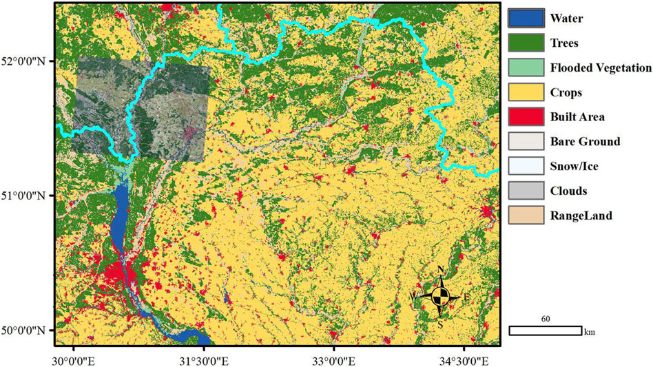
Figure 1. Study area (marked as dark). It lies at the border between Ukraine and Belarus falling within the temperate continental climate zone.

3.2 SAR and optical satellite data

The SAR data used in this study were acquired from the Sentinel-1 satellite. Launched in 2014, the Sentinel-1A satellite carries a 5.4 GHz C-band SAR sensor. The level-1 Interferometric Wide Swath (IW) mode Ground Range Detected (GRD) data were utilized with dual polarization modes (vertical-vertical, and vertical-horizontal, VV and VH). Preprocessing includes thermal noise removal, geometric correction, radiometric calibration, denoising, and topographic correction. The systematic processing chain converted digital number values into geographically linked backscattering coefficients.

Optical data were also employed to support the analysis of SAR data. Analysis of SAR data was conducted separately on single land cover type, for which the land cover classification (or semantic segmentation) is needed. SAR data is not intuitive when interpreting terrain content, as it is difficult to label and can lead to significant errors. Therefore, to ensure the high accuracy of land cover boundaries, optical data were used to extract spatial extents of specified land cover types. Multi-temporal optical data were acquired from multispectral data of the Sentinel-2 satellite. The Sentinel-2 satellite constellation (comprising Sentinel-2A and Sentinel-2B) carries a high-resolution multispectral imager (MSI) designed to provide the timely observation of vegetation, soil, and water, where the level-1C multispectral (MSI) Sentinel-2 data were utilized with blue, green, red, and near infrared (B/G/R/NIR) bands for classification.

3.3 Meteorological data

In addition to the trend analysis, the correlation between scattering coefficient and temperature will also be discussed. The scattering coefficient is directly related to atmospheric density, which is not easily obtained. Given the standard atmospheric distribution model, the current value of atmospheric density is obtained through the formula $\rho =1.293\times \left(P/P_0\right)\times \left(273.15/T\right)$, where $P$ and $P_0$ represent the current and standard atmospheric pressures, respectively, and $T$ represents the current Kelvin temperature. There is generally a stable negative correlation between changes in atmospheric density and changes in temperature. For example, when temperature rises due to seasonal changes, the current air pressure usually decreases, leading to a decrease in air density, and vice versa. Therefore, the air temperature is linked to the scattering coefficient for correlation analysis.

Precipitation is not considered in the analysis. Precipitation affects soil moisture, which in turn influences the VV coefficient. When precipitation saturates soil moisture, the VV coefficient increases by 2–4 dB. Additionally, rainfall can disrupt canopy structures, leading to a short-term increase in the VH coefficient (approximately 3 dB). However, rainfall is not a direct impact factor, as it interacts through soil. Moreover, rainfall is locally observed which complicates the identification of global patterns. More critically, rainfall-induced changes in scattering coefficients represent short-term phenomena that can be considered as the noise in long-term patterns. Therefore, in our analysis, we minimized the impact of rainfall through the averaging operation over large regions.

The meteorological data is sourced from the Integrated Climate Data Set (https://www.ncei.noaa.gov/maps/daily) published by the National Oceanic and Atmospheric Administration (NOAA). The selected meteorological station is located within 100 km of the center of the study area. The weather variables are daily maximum temperature, daily minimum temperature, and daily mean temperature. A total of 174 daily temperature data were extracted from 24-April-2019 to 29-December-2024 with an interval of 12 days.

3.4 Extracting woodland covers via multi-temporal classification

Geographically matched optical images are used to determine the category of land cover, which will be identified pixel by pixel through our previously designed fine-grained multi-scale classification network (FGMCN). High-resolution satellite imagery exhibits rich scale diversity. The scope of woodlands can be either large or small with no fixed scale. Traditional classifiers can only learn features at a given scale. In contrast, the fine-grained multi-scale classifier provides greater flexibility in terms of the scope of woodlands, thereby improving the classification quality.

FGMCN employs convolutional neural networks (CNNs) for feature extraction. We have made experiments on multiple satellite images and concluded that CNNs deliver optimal efficiency in scenarios requiring partial human annotation of image pixels, outperforming Transformers in classification accuracy by using fewer labeled samples. FGMCN utilizes multiscale residual blocks (MRBs) for feature extraction, as illustrated in Figure 2.

Figure 2

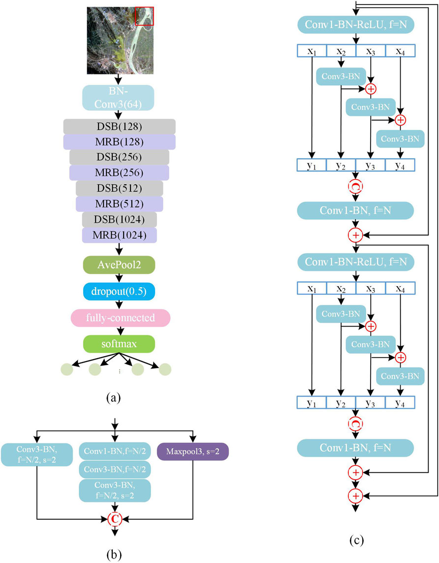
Figure 2. Structure of the classifier to identify woodland. Four DSBs are cascaded for multi-scale downsampling. The four serial convolutions in the MRB identify fine-grained features. (a) main network, (b) downsampling block (DSB), (c) multiscale residual block (MRB).

Within the FGMCN architecture, each MRB incorporates multi-level residual connections and two multiscale residual submodules to achieve discriminative receptive fields at fine-grained levels. Four parallel branches extract features across distinct scales. The MRB constructs hierarchical residual connections within a single residual block, thereby expanding the scope of receptive fields. Consequently, the network dynamically adapts to the most scale-appropriate features for the input image content. The final output maintains identical channel dimensions to the input, with uniform channel allocation across all branches.

Parameters of FGMCN are given for training and inference. The categorical cross entropy loss is used. The batch size is set to 64. The optimization uses stochastic gradient descent (SGD) optimizer and trains 200 epochs. The learning rate is 0.001 in the 101–200 epochs and 0.0005 in the 100–200 epochs. The input patch has $27\times 27$ pixels.

We also employed post-processing to ensure that the extracted land cover types were exactly woodland. In each optical image, sample patches were manually annotated to train FGMCN. The trained network was then used to extract the full woodland extent for that specific image. The overlapping woodland regions obtained from multi-temporal optical images were combined to derive the woodland areas that remained unchanged in land cover class throughout the study period. Although the classification accuracy for woodland is high, misclassifications could still occur in transition zones between classes. To mitigate misclassifications, morphological erosion filtering was applied to remove isolated and marginal labels. Following these processing, a high-precision mask was obtained marking the long-term woodland area.

3.5 Trend analysis methods

We will analyze the annual and seasonal trends of the scattering coefficient. Seasonal analysis gives the conclusions about magnitude changes of the scattering coefficient across different seasons. Before conducting seasonal analysis, an annual trend analysis is preceded to evaluate whether the scattering coefficient exhibits annual stationarity, which will determine the applicability of seasonal analysis methods.

We employed the seasonal Mann-Kendall test to analyze the fluctuation in SAR backscattering coefficients. It compares the changes of the same month across multiple years, and concludes the overall trend across multiple years. As a non-parametric approach, it relies solely on the relative ordering of data values without considering their magnitudes, thereby mitigating impacts from potential seasonal anomalies, missing or undetected values in backscattering coefficients. The length of the time-series backscattering coefficients significantly influences trend detection. Sequences shorter than 5 years may not assess the accurate trend, whereas the excessively long sequences (e.g., longer than 8 years) may smooth trends. Thus, the trend analysis in this study is theoretically reliable which uses every 12 days of backscattering coefficient lasting 5.7 years.

As for the seasonal trend analysis, Fourier transform and Seasonal-Trend decomposition using LOESS (STL decomposition) are possible candidates. Fourier transform can quantify periodic intensity but is only suitable for stationary data. STL decomposition can be applied to non-stationary data. The selection of specific methods depends on the overall annual trend derived from the seasonal Mann-kendall test.

4 Results of trends and correlation

4.1 Area of woodland covers

We evaluated the classification accuracy of the FGMCN algorithm. Testing samples of forest land and non-forest land were manually labeled on the classification map, which are randomly distributed across the entire map and do not overlap with the training map. The classification results were assessed using multiple metrics which are presented in Table 1. The overall accuracy reaches over 95%, which indicates that the classification results are highly reliable. A recall rate of 95.92% means there are few missed classifications, effectively ensuring the integrity of the woodland area. The F1-score shows that the model has no serious bias between misclassification errors and missed classification errors, thus proving that the classification system has good stability and reliability.

Table 1

Table 1. Evaluation of classification results.

The range of the woodland to be analyzed is shown in Figure 3. It is obtained by classifying multi-temporal optical images with a size of 8,$000\times 10$,980 using the FGMCN algorithm and then shrinking the overlapping areas with morphological erosion. Multi-temporal classification eliminates the impact of clouds and land cover changes, and authorize the fidelity of the extracted woodland range. The effective woodland range contains 9,484,574 pixels, with an area of 948 ${\text{km}}^2$, accounting for 10.8% of the entire area.

Figure 3

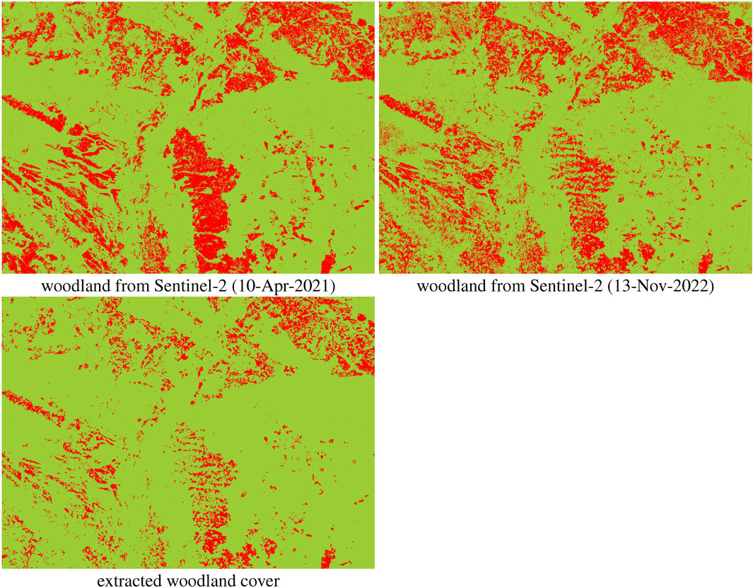
Figure 3. Woodland area extracted from multi-temporal optical images. The extracted woodland cover is from the common pixel locations that are shrunk with morphological filtering to avoid ambiguous labels in transition zones.

4.2 Annual trends from seasonal Mann-Kendall test

The annual and seasonal analysis for the 6-year 12-day-interval scattering coefficient sequences process with the seasonal Mann-Kendall test can be briefly summarized into three main steps: calculating the difference and its corresponding variance month by month, summing them to obtain the total variance, and then deriving the statistic values $\tau$ and the significance level $\alpha$. The fluctuation trend of the scattering coefficient in the time series is jointly determined by these two parameters. $\tau >0$ indicates a possible upward trend, while $\tau <0$ indicates a possible downward trend. $\tau$ needs to be evaluated in combination with $\alpha$. $\alpha$ is a positive value, and the smaller it is, the stronger the significance. Generally, $\alpha \le 0.01$ indicates a high level of significance, while $0.01<\alpha \le 0.1$ indicates significance.

Table 2 provides the annual and seasonal trend of VV, indicating that VV did not exhibit an obvious changing trend in year-on-year variations, either. In the monthly analysis, January and April are evaluated as significant, while other months are non-significant. It is noteworthy that the absolute $\tau$ value reached 0.3846 for both January and April, suggesting drastic environmental fluctuations within the seasons. The remaining months showed alternating positive and negative trends, but none reached the significance level, reflecting significant spatiotemporal heterogeneity in VV changes, which may be related to seasonal precipitation fluctuations and human activity cycles. The overall fluctuation trend shows a slight downward trend, but it is not significant, indicating that the VV scattering coefficient has approximate annual stability.

Table 2

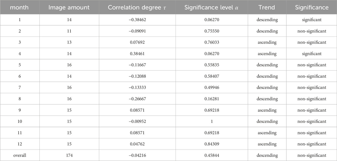
Table 2. Trends of VV intensity by seasonal Mann-Kendall Test.

Table 3 provides the annual trend of VH, indicating that VH did not show an obvious trend in the year-on-year changes. In the monthly analysis, all months did not reach the significance level. The absolute $\tau$ value reached 0.2747 in January. The monthly trends of VH are very similar to those of VV, with 10 out of 12 months being consistent, and deviations only occurring in September and November. The overall fluctuation trend shows a slight downward trend, but it is not significant, indicating that the VH scattering coefficient has higher annual stability than VV.

Table 3

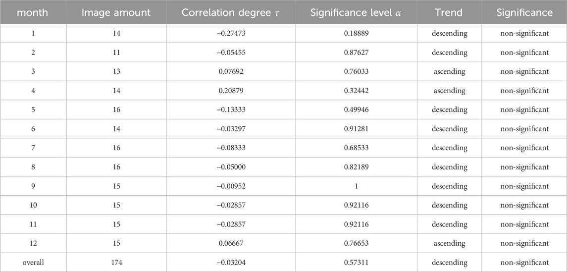
Table 3. Trends of VH intensity by seasonal Mann-Kendall Test.

To conclude, both VH and VV exhibited overall weakly decreasing trends during the study period, but the statistical significance was insufficient to exclude the possibility of random fluctuations. At the monthly scale, both displayed the synchronization of trend changes in most months. Notably, VV showed a significant decreasing trend in January and a significant increasing trend in April. The most consistent time throughout multiple years occurs in October for VV and September for VH, respectively.

A comparison of Tables 2,3 reveals the seasonal sensitivity of different polarization modes to woodland. The co-polarization information recorded by VV is dominated by direct surface scattering, making it more sensitive to changes in bare soil moisture. The cross-polarization information recorded by VH primarily originates from volume scattering and secondary reflections, showing high sensitivity to vegetation structural changes such as biomass and canopy density. In most months, the $\alpha$ value of VV is lower than that of VH except in May, October, and December. This reflects that the cross-polarization mode of Sentinel-1 can capture forest canopy dynamics more promptly than the co-polarization mode.

4.3 Seasonal trends from STL decomposition

Since the seasonal Mann-Kendall test indicates weak fluctuations in the annual trends, it is not a stationary random process for the scattering coefficients. In this case, analysis with Fourier transform would introduce errors, so we employ STL decomposition to analyze seasonal trends. The STL model employs locally weighted regression to decompose time series data into three components: the trend-cycle component, the seasonal component, and the residual component. The trend-cycle component describes the overall directional changes of the data on a long-term scale, and captures slow and persistent variations. The seasonal component represents the fluctuating patterns that repeat within a fixed period in the data. The residual component stands for random fluctuations or measurement errors that cannot be explained by trends or seasonality in the model.

Figure 4 presents the results of STL decomposition, where VV and VH give similar trends. The trend-cycle components show that the overall scattering coefficient experienced a slight decrease in 2023 and 2024, with a magnitude ranging from approximately 3%–6%. Seasonal analysis reveals an obvious annual periodicity: 1) The scattering intensity hits the highest in summer and the lowest in winter; 2) Local maximum may occur in early winter; and 3) The recovery from the local minimum is rapid which occurs in early spring. The residuals indicate anomalies at the end of 2019 and the end of 2022. The anomaly at the end of 2019 may be related to the extremely rare drought persistent from summer to autumn in 2019, which led to insufficient soil moisture and made the attenuation of scattering intensity less than expected. In the winter of 2022, affected by the triple La Niña phenomenon, Ukraine experienced its coldest winter in decades, which resulted in the scattering coefficient being lower than that in normal years.

Figure 4

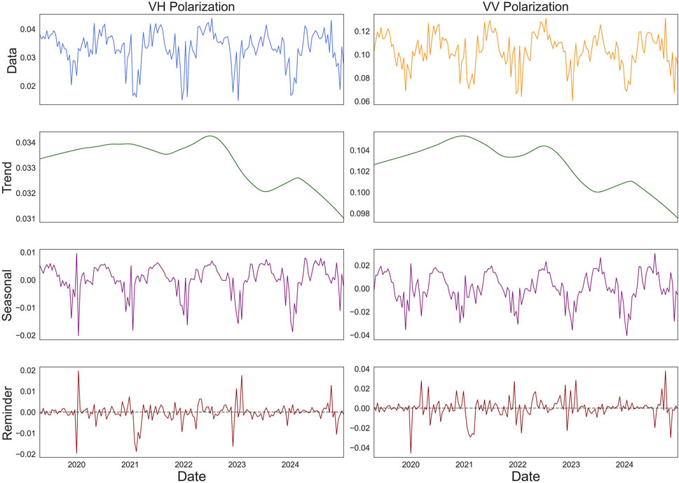
Figure 4. Results of STL decomposition. The left is for VH and the right is for VV. The curves from top to bottom are in turn the intensity data, the trend-cycle component, the seasonal component, and the residual component. Seasonal cycles are clear in the third row.

4.4 Correlation to temperature

The Pearson correlation coefficient is used to assess the relationship between the scattering coefficients and temperatures, while the Pearson significance value describes the statistical significance (less than 0.05 is generally considered significant), as presented in Table 4. For VV polarization, the correlation to daily minimum, maximum, and average temperatures are evaluated as 0.7489, 0.7068, and 0.7554, respectively. For VH polarization, the corresponding coefficients are 0.7571, 0.7161, and 0.7612, respectively. All correlation coefficients passed the significance test, indicating a statistically significant positive correlation between temperatures and SAR backscattering. Notably, daily average temperature shows higher correlation to scattering coefficients than daily maximum and minimum temperatures. The correlation coefficients related to VV are all slightly smaller than those related to VH. Combined with the results of time series analysis, both VV and VH polarization data exhibited a seasonal pattern: backscattering intensity peaked in summer (June–July) and reached its lowest point in winter, demonstrating high synchronization with the interannual fluctuations in temperature.

Table 4

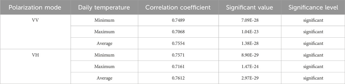
Table 4. Pearson correlated coefficient between temperatures and backscattering coefficients.

The dynamic relationship between temperature and backscatter coefficients is drawn in Figure 5, which can be explained by ecophysical mechanisms. In summer, the dielectric properties of woodland trees are enhanced because high temperatures promote photosynthesis and transpiration, leading to canopy biomass accumulation and increased leaf water content. This change enhances the intensity of volume scattering of SAR signals. Especially in dense canopies, multiple interactions between radar waves and branches/leaves cause simultaneous increases in cross-polarization (VH) and co-polarization (VV) backscatter coefficients. In winter, simplified canopy structure and reduced biomass make surface scattering dominant. Backscatter coefficients are then susceptible to environmental factors such as snow cover, freeze-thaw cycles, or soil moisture changes, causing values to be significantly lower than those in the growing seasons. The correlation to daily average temperature is higher than that of daily maximum and minimum temperature, which is accounted for the cumulative thermal effect of physiological activities in trees, whereas extreme temperatures are interfered by short-term meteorological events such as abrupt cloud changes and heavy precipitation.

Figure 5

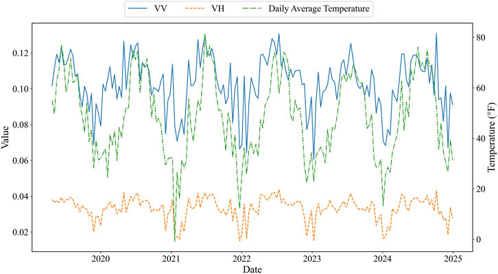
Figure 5. Relations between backscattering coefficients and temperatures. They exhibit roughly the same trend at the peaks and troughs.

For dual-polarization (VV + VH) Sentinel-1 data, Nasirzadehdizaji et al. (2019) suggested the Radar Vegetation Index (RVI) which is calculated by Equation 1 as

$\mathrm{R}\mathrm{V}\mathrm{I}=\frac{4{\sigma }_{\mathrm{V}\mathrm{H},\mathrm{l}\mathrm{i}\mathrm{n}\mathrm{e}\mathrm{a}\mathrm{r}}^0}{{\sigma }_{\mathrm{V}\mathrm{V},\mathrm{l}\mathrm{i}\mathrm{n}\mathrm{e}\mathrm{a}\mathrm{r}}^0+{\sigma }_{\mathrm{V}\mathrm{H},\mathrm{l}\mathrm{i}\mathrm{n}\mathrm{e}\mathrm{a}\mathrm{r}}^0},(1)$

where ${\sigma }_{\mathrm{V}\mathrm{V},\mathrm{l}\mathrm{i}\mathrm{n}\mathrm{e}\mathrm{a}\mathrm{r}}$ and ${\sigma }_{\mathrm{V}\mathrm{H},\mathrm{l}\mathrm{i}\mathrm{n}\mathrm{e}\mathrm{a}\mathrm{r}}$ denote the linear backscattering intensity, and the RVI value ranges typically between 0 and 1. Values close to 0 indicate barren landscapes (such as bare land and water surfaces), while larger values (usually larger than 0.5-0.6) denote dense vegetation landscapes.

Figure 6 shows that the RVI values fall within the range [0.8,1.0], indicating that the woodland is characterized by dense vegetation and complex structure, with volume scattering as the dominant mechanism. The ratio of VH to VV backscattering coefficients is concentrated in the range [0.2,0.4], which further confirms that the vegetation scattering characteristics in this area are dominated by a moderate depolarization effect. These two types of indicators exhibit a highly consistent synergistic variation trend over the temporal dimension. Particularly in winter, both indicators show a significant decline: the RVI value drops sharply to approximately 0.7, and the VH/VV ratio also decreases synchronously. These variation patterns are consistent with the land surface temperature time series, as the time node of the sudden decline corresponds to the period of persistently low temperatures. This indicates that the radar backscattering intensity and polarization ratio have an obvious response to temperature changes, implying the potential regulatory role of thermal conditions in vegetation dielectric properties, phenological status, or surface ice/snow cover conditions.

Figure 6

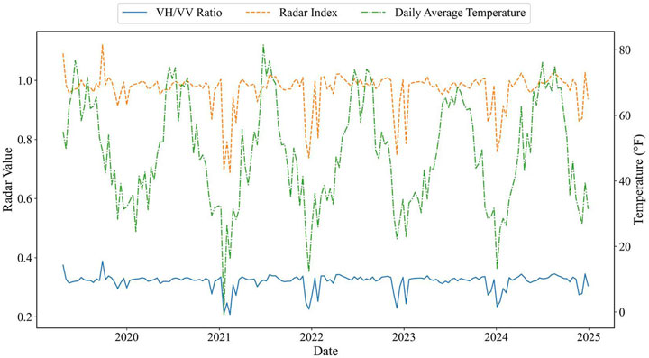
Figure 6. Relations between backscattering ratio, radar index, and average temperature. High correlation exists between VH/VV and radar index which both reflects the visibility of dense trees.

The heterogeneity of finer woodland types affects the correlation between temperature and scattering intensity. With coniferous-broadleaf mixed woodland as the main type, the study area exhibits structural heterogeneity. Coniferous forests, due to their advantage in vertical structure, tend to generate strong volume scattering in the VV polarization channel, while their scattering in the VH polarization channel is dominated by canopy biomass. In contrast, broadleaf woodland canopies are more likely to induce depolarization effects due to randomness, and are more sensitive to changes in soil humidity. Although this heterogeneity does not dominate the statistical significance of the temperature response across the entire study area, it weakens the consistency of trends in local regions.

5 Predicting scattering coefficient in woodland with explainable neural networks

5.1 Model structure

The results in Section 4 indicate the seasonal repetition in SAR scattering coefficients over woodland covers, which can be modeled using sequence-based networks. Commonly used sequence modeling methods include Autoregressive Integrated Moving Average (ARIMA) model, Recurrent Neural Network (RNN), Long Short-Term Memory (LSTM) network, Transformer, Informer, Mamba, etc. Considering that seasonal trends are included and the length of input data is limited, we employ Autoformer (Wu et al., 2021; 2023) as the modeling basis. Autoformer is a modified Transformer network addressing the bottlenecks of complex temporal patterns and computational efficiency. Two important innovations were proposed in Autoformer. First, sequence decomposition in the preprocessing step is integrated into internal operators to establish a progressive mechanism gradually separating long-term trends and seasonal components from intermediate prediction variables. Second, conventional self-attention is replaced with an auto-correlation mechanism, which computes subsequence similarities driven by sequence periodicity to discover and integrate sequence dependency. The first solution enhances analytical capabilities for temporal dynamics, while the second solution reduces computational complexity.

Figure 7 illustrates the structure of the network, where the encoder receives multi-source inputs. The input is formed by concatenating the VV scattering coefficient sequence, the VH scattering coefficient sequence, and the daily average temperature sequence, resulting in an input tensor with a dimension of $R^{L_{\text{TrainLen}}\times \left(d_{\text{VV}}+d_{\text{VH}}+d_{\text{temperature}}\right)}$, where $L_{\text{TrainLen}}$ represents the sequence length of input. This fusion strategy leverages the high correlation among the three types of data and preserves the spatiotemporal association between surface physical properties and thermodynamic states.

Figure 7

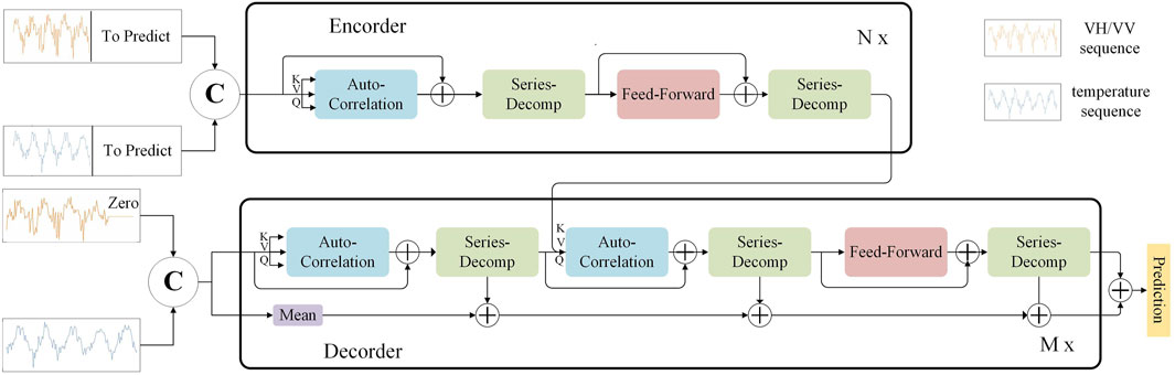
Figure 7. Framework of the model for prediction of SAR scattering coefficients. The complete SAR data was used for training. During inference, the data at unknown moments is input as 0, and the SAR sequence is generated by the decoder.

The decoder adopts a dual-branch initialization mechanism to guide prediction. The first branch initializes the VV/VH data to be predicted as a zero tensor, and concatenates it with temperature data at the prediction days to form a placeholder input of dimension $R^{L_{\text{PredLen}}\times \left(d_{\text{VV}}+d_{\text{VH}}+d_{\text{temperature}}\right)}$, where $L_{\text{PredLen}}$ denotes the prediction length. The second branch calculates the mean value of the concatenated tensor along the time dimension to generate an aggregated representation with preserved dimensions. The inputs from both branches are jointly fed into the decoder, and progressive information refinement is achieved through cascaded decomposition blocks. This design inherits three core mechanisms of Autoformer. First, the Series Decomp block separates potential trends through a moving average operation $x_t=\mathrm{A}\mathrm{v}\mathrm{g}\mathrm{P}\mathrm{o}\mathrm{o}\mathrm{l}\left(\mathrm{P}\mathrm{a}\mathrm{d}\mathrm{d}\mathrm{i}\mathrm{n}\mathrm{g}\left(x\right)\right)$. Second, the auto-correlation mechanism models subsequence-level dependencies by calculating the time-delay similarity $R_{xx}\left(\tau \right)=F^{-1}\left(S_{xx}\left(f\right)\right)$ based on fast Fourier transform. Last, time delay aggregation rolls and aligns similar phase points according to the top-k periods ${\tau }_1,\dots ,{\tau }_k$.

The internal data flow of the framework strictly follows the operator sequence of the original Autoformer. The encoder gradually strips off the trend components of the input data through stacking $N$ layers, focusing on the extraction of seasonal features. The decoder alternately performs autocorrelation operations and decomposition operations through an $M$-layer structure, and its output layer linearly superimposes the refined seasonal term and the accumulated trend term to generate the final prediction. This study introduces temperature covariates to enhance multimodal representation capabilities, and uses zero-initialized placeholders to realize the autoregressive prediction of VV/VH values in the prediction days. While maintaining the computational complexity of $O(L\log L)$ of the original model, it improves the physical interpretability of long-term prediction of surface parameters.

5.2 Explainable consistency between temporal trends and model structure

The Autoformer model has good interpretability for our work. The key innovations–progressive sequence decomposition, autocorrelation calculation, and subsequence attention mechanism–match well with the issue of SAR intensity evolution trends. The link between the issue and the model is discussed.

First, Autoformer adopts time series decomposition as a basic operation module of the deep model rather than a preprocessing step, decomposing hidden variables layer by layer to extract long-term trend terms and seasonal terms. This structure makes the trend and seasonal components of the prediction results traceable, enhancing the transparency of the model’s behavior. Consistent with the key design of the model, the results of the seasonal Mann-kendall test and the STL decomposition in Section 4 have verified the existence of long-term trends and seasonal trends in scattering coefficients. In addition, this progressive decomposition enables the model to explicitly separate patterns of different time scales, ensuring that datasets constructed using different revisiting periods can be modeled.

Second, Autoformer uses subsequence-level correlation of the autocorrelation mechanism to replace the traditional point-to-point self-attention, further meeting the needs of periodic sequences. A large number of calculations in self-attention are wasteful for periodic SAR scattering coefficient, because there is weak correlation between two moments across seasons. The autocorrelation mechanism calculates sequence periodicity through Fast Fourier Transform (FFT) and aggregates similar subsequences based on time-delay dependence. This periodic intensity can be visualized, and the intensity of dominant cycles (such as daily, weekly, or monthly) in the time series can be intuitively displayed through autocorrelation weights, reflecting the coherence of scattering intensity.

Finally, the subsequence aggregation in the network facilitates the input of meteorological conditions. The weighted aggregation of subsequences with similar phases, such as associating data at the same moment in different cycles, can form a physically meaningful expression of dependencies. This enables the network to discover the correlation between daily average temperature and scattering intensity and use it to guide predictions.

The coupling between the model and data demonstrates the completeness of this work in providing explainable model. First, seasonal patterns were summarized through trend analysis. Second, a high correlation with average temperature was identified via correlation analysis. Finally, seasonal trends and temperature correlations were subtly integrated into the network. These efforts have endowed the sequence neural network we used with interpretability. In contrast, existing neural network modeling generally neglects the explicit analysis of the intrinsic properties of data, thus lacking credible model interpretability.

5.3 Scheme of validation

The details of training and inference are given. Training data consists of 9,484,574 pairs of VV/VH sequences from 143 images between April 2019 and December 2023 of 12-day, encompassing complete tree growth cycles and diverse interannual climate variations. The testing utilized 31 observations from the year of 2024 to validate the model’s prediction capability for unseen time periods. During training, the Mean Square Error (MSE) metric served as the loss function. The optimization was performed using the Adam optimizer with the initial learning rate as 1e-4. The batch size is 32. The early stopping mechanism was used to prevent overfitting.

The input, output, and conditional information of the network are also provided. The length of the input sequence is 30, and the output length is 3. In other words, data from the previous 30 time instants are used to predict the data for the next three time instants in each generation. In each inference, an average temperature sequence is fed into the network along with the SAR sequence.

The test includes two types. One is the original data sequence, which contains 9.48 million sequences. The other is 9,484 average sequences obtained by randomly grouping these sequences and taking the average, with each group consisting of 1,000 pixel locations. The averaging operation roughly eliminates the heterogeneity differences caused by random structural differences (e.g., canopy shapes) and meteorological events (e.g., local rainfall). Root Mean Square Error (RMSE) and Mean Absolute Error (MAE) are used to evaluate the prediction results.

5.4 Prediction results

The evaluation scores on the group average intensity are first given. For VV, the RMSE deviation is 0.006070, and the MAE deviation is 0.005165. For VH, the RMSE deviation is 0.001615, and the MAE deviation is 0.001306. These errors are almost neglectable, considering the average scattering coefficients are 0.1038 for VV and 0.0337 for VH, respectively. The average RMSE diviations are within 6% by dividing the average intensities. These scores indicate that the sequence prediction model has a good ability to capture the changes in the average backscatter coefficient.

To visually evaluate the model’s prediction performance, nine samples were randomly selected from all samples for display. The curves are shown in Figures 8, 9 for VV and VH, respectively. The ground truth and predicted values are distinguished by colors and line styles. The visualization results in Figures 8, 9 indicate that the prediction curves of groups highly coincide with the ground truth curves at most key phenological moments, such as the start of the growing season, peak, and senescence period. The seasonal fluctuation of backscattering coefficients are successfully captured.

Figure 8

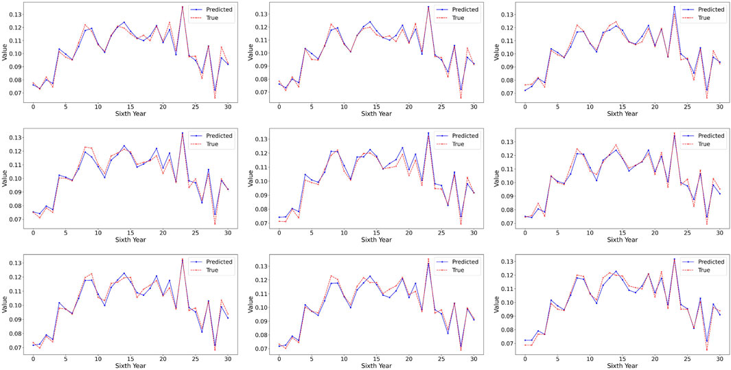
Figure 8. Prediction results of the VV scattering coefficients in grouped locations.

Figure 9

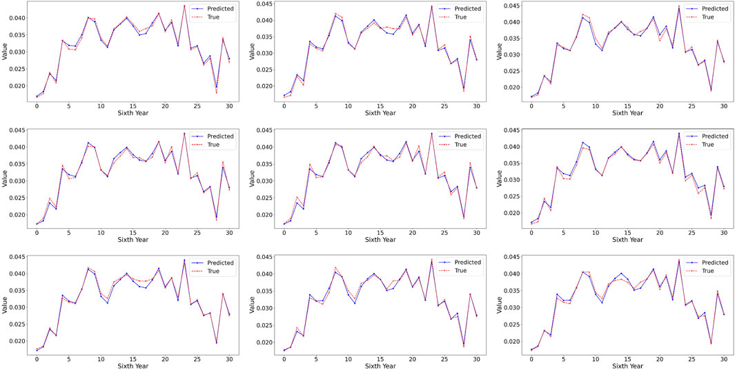
Figure 9. Prediction results of the VH scattering coefficients in grouped locations.

As for the pixel-wise prediction, evaluation was made for VH and VV over 9.48 million samples. For VV, the average RMSE is 0.035036 and the average MAE is 0.026703. For VH, the average RMSE is 0.012932 and the average MAE is 0.009949. These errors are at low values. The relative errors are around 30% by dividing RMSE by the mean values. Random meteorological conditions and complex ground structures make deviations unavoidable. These errors fully indicate that our model can reflect the general trend of the woodland scattering coefficient. Figures 10, 11 present nine samples of the prediction results for pixel-wise prediction. These figures show the ground truth values of 60 time points from January 2023 to December 2024, as well as the prediction results of 30 time points from January 2024 to December 2024. To conclude, the changing trends of the prediction are roughly the same as those of the ground truth. In the prediction interval of the sixth year (the right of the vertical dashed line), the model accurately reproduces key turning points of spring green-up and autumn leaf fall. Individual peaks exhibit a slight lag of approximately two to 4 weeks, reflecting the response mechanism between tree growth and accumulated temperature.

Figure 10

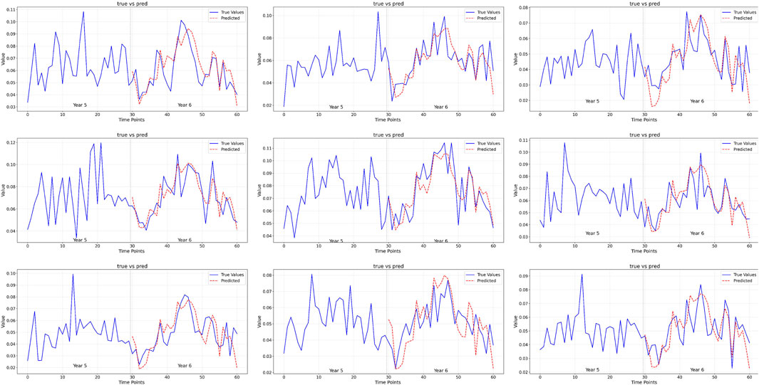
Figure 10. Prediction results of the VV scattering coefficients in single locations.

Figure 11

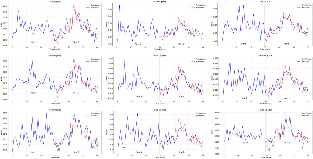
Figure 11. Prediction results of the VH scattering coefficients in single locations.

5.5 Performance comparison

To evaluate the performance of Autoformer, we compared it with Informer and LSTM which are two types of mainstream sequence models. All methods were set with a prediction length of three. Table 5 presented the evaluated experimental results, which shows that Autoformer has significant advantages in modeling the issue in this study. For the VV band, the RMSE values of LSTM and Informer are 40.6% and 37.2% higher than that of Autoformer, respectively. For the VH band, the RMSE values of LSTM and Informer are 43.6% and 35.8% higher than that of Autoformer, respectively. In summary, our experiment shows that Autoformer significantly outperforms the classical LSTM and Transformer-based Informer in modeling time-series scattering intensity. This verifies the unique advantage of Autoformer in capturing the dynamic characteristics of microwave scattering intensity.

Table 5

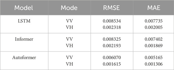
Table 5. Comparison of sequence prediction algorithms.

5.6 Explainable analysis

The explainability of our model differs from general concept. The explainability of neural networks usually refers to understanding the specific internal decision-making mechanisms of the model through post analysis such as feature importance and attention maps. However, this analysis has limitations, as it often involves indirect understanding based on an inherent black box, and the explainability itself may be uncertain due to weak connections to the physical laws behind the data. To enhance explainability, we conducted data analysis-based modeling in this work. Our explainability focuses more on the model’s design basis instead of explaining why the model makes a certain prediction after training. To conclude, we use statistical evidence to ensure that the rationality and reliability of the modeling process for explainability.

To deeply analyze the decision-making mechanism of the Autoformer model, we adopted the Integrated Gradients (IG) method for explainable analysis. The feature values calculated by IG quantify the contribution of each feature to the model’s predictions. A positive value indicates that the feature is positively correlated with the predicted value, and an increase in this feature will raise the predicted quality. A negative value indicates that the feature is negatively correlated with the predicted value, and an increase in this feature will lower the predicted accuracy. The analysis was performed on the VV mode focused on a multivariate input sequence containing 30 steps, covering time-series SAR (Feature 1) and daily average temperature (Feature 2).

The IG analysis presented in Figures 12, 13 reveals the dynamic contribution patterns of each feature across the temporal dimension. For Feature 1 (SAR sequence in Figure 12), the maximum positive attribution value is observed at time step 10, indicating that the feature information at this moment exerts the strongest positive driving effect on the prediction result. In the time step range of 18–22, the attribution value remains consistently negative, which suggests that an increase in the feature value during this period will inhibit the prediction output. Notably, the attribution values of the recent time steps approach zero since step 25, which is consistent with the general rule in sequence prediction that the influence of long-term features usually diminishes. For Feature 2 (daily average temperature in Figure 13), it reaches a positive attribution peak at step 11, which serves as a key positive reference point for the model’s prediction. It demonstrates a stable positive contribution in the step between five and 15, while transitioning to a stable negative impact between 20 and 25 steps. Within the 10 to 12 steps, both features exhibit a synergistic enhancement effect.

Figure 12

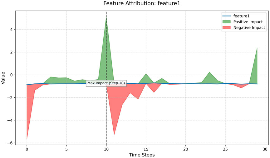
Figure 12. Dynamic contributions of feature 1 (time-series VV coefficients). The maximum positive impact is at step 10. A positive value indicates a positive correlation between the feature and the predicted value, and vice versa.

Figure 13

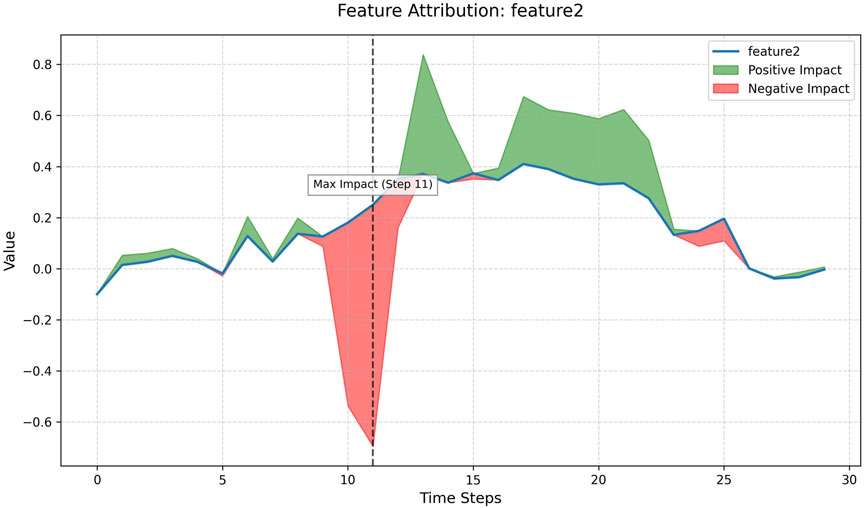
Figure 13. Dynamic contributions of feature 2 (daily average temperature). The maximum negative impact is at step 11. A positive value indicates a positive correlation between the feature and the predicted value, and vice versa.

6 Discussions

6.1 Impact of window length for seasonal analysis

The influence of STL’s window length on the analysis is revealed here. Based on a 12-day revisit cycle, the number of annual observation points is calculated as $365/12\approx 30.4$, among which the closest odd number, 31, is adopted as the seasonal period. This enables the seasonal component to accurately reflect the annual cyclic pattern. The optimal value of the LOESS window length can be determined through systematic sensitivity tests. The test range covers odd-numbered windows from seven to 25, with the minimization of residual variance serving as the selection criterion.

Table 6 presents the results of the sensitivity analysis against the LOESS window length. For both VH and VV data, a LOESS window length of seven yields the minimum residual variance (0.000094 for VV and 0.000018 for VH). As the window length increases, the residual variance shows a monotonic increase. This indicates that a larger LOESS window length leads to over-smoothing of the seasonal signal by keeping more information in the residual term. The seasonal strength of VH fluctuates between 0.609 and 0.620, with the maximum value occurring at a LOESS window length of nine. In contrast, the seasonal strength of VV decreases significantly from 0.6797 to 0.6475 representing a decrease of 4.7%. To conclude, seven is the optimal LOESS window length for the analysis task.

Table 6

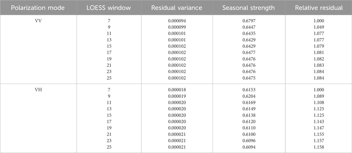
Table 6. Seasonal analysis against LOESS window length.

6.2 Impact of prediction length

The prediction length is changed to evaluate the robustness of the Autoformer model. The prediction length is extended to 15 steps allowing for prediction across 6 months. Table 7 presents the evaluated experimental results, which shows that Autoformer exhibits good adaptability over longer prediction horizons. Even when the prediction length significantly exceeds the initial short period, the model can still maintain its prediction accuracy without linear growth or collapse of errors. This strongly demonstrates that Autoformer is well-suited to our problem and possesses the robustness to capture long-term temporal dependencies.

Table 7

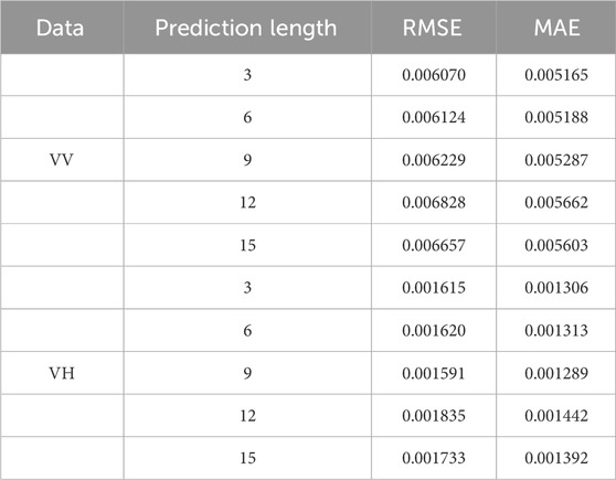
Table 7. Prediction accuracy against prediction length.

The two polarization modes show different responses to prediction length. The error of VV shows a mild increase as the prediction length increases, but exhibits stabilization at the ${15}^{th}$ step (approximately 6 months). For VH data, when the prediction length increases from three steps to nine steps, the error even decreases slightly. When the prediction length is further extended to 12 steps (approximately 4.8 months), the VH error rises, but tends to decrease again at the ${15}^{th}$ step. As the prediction length gradually increases in both trends, the prediction error remains stable, with no cumulative error or sharp decline in accuracy observed.

6.3 Impact of spatial heterogeneity

The RMSE errors were geolocated to form the spatial distribution maps of RMSE as shown in Figures 14, 15, which reveal the spatial heterogeneity within the prediction results. The RMSE maps exhibit a spatial trend of gradual increasing from south to north. This obvious north-south difference indicates that the prediction performance of the model is not spatially uniform, and its ability to capture the dynamic changes of backscattering signals in the woodland areas of the northern part of the study area is relatively weaker than that in the southern region.

Figure 14

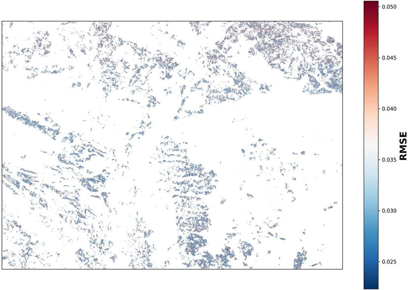
Figure 14. Spatial distribution of the VV prediction errors. The northern locations show more RMSE deviations.

Figure 15

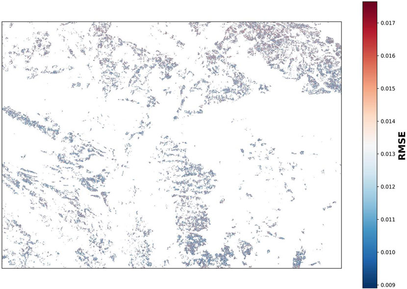
Figure 15. Spatial distribution of the VH prediction errors. The northern locations show more RMSE deviations.

The spatial heterogeneity within RMSE maps may be driven by a variety of potential geospatial factors. Possible reasons are more complex terrain (such as changes in elevation gradients or differences in slope), a distinct distribution of woodland types, spatiotemporal variability in soil moisture, or stronger atmospheric and phenological processes (such as the frequency and intensity of precipitation events). All these factors can significantly affect the response mechanism of Sentinel-1 SAR signals and their time-series characteristics. The current prediction model fail to fully characterize the composite effects of all driven factors in the northern region, leading to a systematic increase in prediction uncertainty. This result suggests that future model should focus on integrating key environmental covariates or spatial structural features that can explain this north-south distinction.

7 Conclusion

This paper analyzed and explicitly modelled the trends of woodland SAR scattering coefficients of dual-polarized Sentinel-1A data. Taking the woodland areas in the border region of Ukraine and Belarus as the study area, we constructed a sequence of 174 consecutive SAR images spanning from April 2019 to December 2024 using Sentinel-1A GRD data with a 12-day revisit cycle. We extracted the forest cover area in these images by classifying geographically matched multi-temporal Sentinel-2 multispectral images using a fine-grained multi-scale convolutional neural network. A total of 9.48 million pairs of VV/VH scattering coefficient sequences were extracted for analysis. For the sequence data, we conducted annual trend analysis with the seasonal Mann-Kendall test and evaluated the annual changes in scattering intensity. The seasonal-trend decomposition using LOESS presented obvious seasonal trend. The correlation analysis indicated a high correlation between the average temperature and the average scattering intensity. Based on these conclusions, we constructed a scattering intensity prediction model using a neural network, which predicts the scattering intensity at unknown moments by combining the scattering intensity sequences at known moments and the temperature at unknown moments. The evaluation of the annual sequence synthesis results showed that the RMSE error of the average intensity was within 6% towards the average intensity. These studies on trend analysis and modeling temporal trend for woodland demonstrate the potential of generating SAR sequences pursuing quantitative accuracy, and set an example for time-series research on other land cover categories.

Data availability statement

The original contributions presented in the study are included in the article/supplementary material, further inquiries can be directed to the corresponding author.

Author contributions

ZY: Data curation, Formal Analysis, Software, Writing – original draft. HZ: Software, Writing – original draft. PK: Data curation, Writing – original draft. JW: Conceptualization, Funding acquisition, Investigation, Methodology, Resources, Supervision, Writing – review and editing.

Funding

The author(s) declare that financial support was received for the research and/or publication of this article. This research was supported by the National Natural Science Foundation of China (No. 42267070).

Conflict of interest

The authors declare that the research was conducted in the absence of any commercial or financial relationships that could be construed as a potential conflict of interest.

Generative AI statement

The author(s) declare that no Generative AI was used in the creation of this manuscript.

Any alternative text (alt text) provided alongside figures in this article has been generated by Frontiers with the support of artificial intelligence and reasonable efforts have been made to ensure accuracy, including review by the authors wherever possible. If you identify any issues, please contact us.

Publisher’s note

All claims expressed in this article are solely those of the authors and do not necessarily represent those of their affiliated organizations, or those of the publisher, the editors and the reviewers. Any product that may be evaluated in this article, or claim that may be made by its manufacturer, is not guaranteed or endorsed by the publisher.

References

Albanesi, E., Bernoldi, S., Dell’Acqua, F., and Entekhabi, D. (2021). Covariation of passive-active microwave measurements over vegetated surfaces: case studies at l-band passive and l-c- and x-band active. Remote Sens. 13, 1786. doi:10.3390/rs13091786

CrossRef Full Text | Google Scholar

Amani, M., Poncos, V., Brisco, B., Foroughnia, F., DeLancey, E. R., and Ranjbar, S. (2021). Insar coherence analysis for wetlands in Alberta, Canada using time-series sentinel-1 data. Remote Sens. 13, 3315. doi:10.3390/rs13163315

CrossRef Full Text | Google Scholar

Baek, W.-K., and Jung, H.-S. (2019). A review of change detection techniques using multi-temporal synthetic aperture radar images. Korean J. Remote Sens. 35, 737–750. doi:10.7780/KJRS.2019.35.5.1.10

CrossRef Full Text | Google Scholar

Bai, X., He, B., Li, X., Zeng, J., Wang, X., Wang, Z., et al. (2017). First assessment of sentinel-1a data for surface soil moisture estimations using a coupled water cloud model and advanced integral equation model over the tibetan Plateau. Remote Sens. 9, 714. doi:10.3390/rs9070714

CrossRef Full Text | Google Scholar

Bao, J., Yu, W. M., Yang, K., Liu, C., and Cui, T. J. (2024). Improved few-shot SAR image generation by enhancing diversity. IEEE J. Sel. Top. Appl. Earth Observations Remote Sens. 17, 3394–3408. doi:10.1109/JSTARS.2024.3352237

CrossRef Full Text | Google Scholar

Bourgeau-Chavez, L. L., Grelik, S. L., Battaglia, M. J., Leisman, D. J., Chimner, R. A., Hribljan, J. A., et al. (2021). Advances in amazonian peatland discrimination with multi-temporal palsar refines estimates of peatland distribution, c stocks and deforestation. Front. Earth Sci. 9, 676748. doi:10.3389/feart.2021.676748

CrossRef Full Text | Google Scholar

Chen, Q., Zhou, Z.-F., Wang, L.-Y., Dan, Y.-S., and Tang, Y.-T. (2020). Surface soil moisture retrieval using multi-temporal sentinel-1 SAR data in karst rocky desertification area. J. Infrared Millim. Waves 39, 626–634. doi:10.11972/j.issn.1001-9014.2020.05.014

CrossRef Full Text | Google Scholar

Erten, E., Rossi, C., and Yuezueguellue, O. (2015). Polarization impact in tandem-x data over vertical-oriented vegetation: the paddy-rice case study. IEEE Geoscience Remote Sens. Lett. 12, 1501–1505. doi:10.1109/lgrs.2015.2410339

CrossRef Full Text | Google Scholar

Fernandez-Carrillo, A., McCaw, L., and Tanase, M. A. (2019). Estimating prescribed fire impacts and post-fire tree survival in eucalyptus forests of Western Australia with l-band SAR data. Remote Sens. Environ. 224, 133–144. doi:10.1016/j.rse.2019.02.005

CrossRef Full Text | Google Scholar

Fu, S., Xu, F., and Jin, Y.-Q. (2021). Reciprocal translation between SAR and optical remote sensing images with cascaded-residual adversarial networks. Sci. China-Information Sci. 64, 122301. doi:10.1007/s11432-020-3077-5

CrossRef Full Text | Google Scholar

Guo, Q., Xu, H., and Xu, F. (2023). Causal adversarial autoencoder for disentangled SAR image representation and few-shot target recognition. IEEE Trans. Geoscience Remote Sens. 61, 1–14. doi:10.1109/TGRS.2023.3330478

CrossRef Full Text | Google Scholar

Guo, X., Tian, T., Tan, H., Fan, W., and Zhou, F. (2024a). A deceptive jamming technology against SAR based on optical-to-SAR template translation. IEEE Trans. Aerosp. Electron. Syst. 60, 5715–5729. doi:10.1109/taes.2024.3399195

CrossRef Full Text | Google Scholar

Guo, X., Yin, J., Li, K., and Yang, J. (2024b). Fine classification and phenological analysis of rice paddy based on multi-temporal general compact polarimetric SAR data. Front. Plant Sci. 15, 1391735. doi:10.3389/fpls.2024.1391735

PubMed Abstract | CrossRef Full Text | Google Scholar

Haldar, D., Rana, P., Yadav, M., Hooda, R. S., and Chakraborty, M. (2016). Time series analysis of co-polarization phase difference (Ppd) for winter field crops using polarimetric c-band SAR data. Int. J. Remote Sens. 37, 3753–3770. doi:10.1080/01431161.2016.1204024

CrossRef Full Text | Google Scholar

Jain, S., Khati, U., and Kumar, V. (2024). “SAR time-series for pod formation detection,” in IEEE international geoscience and remote sensing symposium (IGARSS). IEEE international symposium on geoscience and remote sensing IGARSS, 4192–4195.

Google Scholar

Ju, M., Niu, B., and Hu, Q. (2023). Sargan: a novel SAR image generation method for SAR ship detection task. Sensors J. 23, 28500–28512. doi:10.1109/JSEN.2023.3323322

CrossRef Full Text | Google Scholar

Kirillov, A., Mintun, E., Ravi, N., Mao, H., Rolland, C., Gustafson, L., et al. (2023). Segment anything. arXiv:2304.02643. doi:10.48550/arXiv.2304.02643

CrossRef Full Text | Google Scholar

Li, K., Luan, S., and Zhou, D. (2020). “An optical-to-SAR transformation method for SAR ship image augmentation,” in 3rd IEEE international conference on information communication and signal processing (ICICSP), 264–268.

Google Scholar

Li, J., Smith, R., and Grote, K. (2023). Analyzing spatio-temporal mechanisms of land subsidence in the parowan valley, Utah, USA. Hydrogeology J. 31, 293–311. doi:10.1007/s10040-022-02583-5

CrossRef Full Text | Google Scholar

Liu, Y., Wang, B., Sheng, Q., Li, J., Zhao, H., Wang, S., et al. (2023a). Dual-polarization SAR rice growth model: a modeling approach for monitoring plant height by combining crop growth patterns with spatiotemporal SAR data. Comput. Electron. Agric., 215. doi:10.1016/j.compag.2023.108358

CrossRef Full Text | Google Scholar

Liu, Y., Zhang, Y., Zhao, F., Ding, R., Zhao, L., Niu, Y., et al. (2023b). Multi-source SAR-Based surface deformation monitoring and groundwater relationship analysis in the yellow river Delta, China. Remote Sens. 15, 3290. doi:10.3390/rs15133290

CrossRef Full Text | Google Scholar

Liu, W., Shi, T., Zhao, Z., and Yang, C. (2025). Mapping coastal soil salinity and vegetation dynamics using sentinel-1 and sentinel-2 data fusion with machine learning techniques. IEEE J. Sel. Top. Appl. Earth Observations Remote Sens. 18, 14203–14214. doi:10.1109/jstars.2025.3552436

CrossRef Full Text | Google Scholar

Mahmud, M. S., Howell, S. E. L., Geldsetzer, T., and Yackel, J. (2016). Detection of melt onset over the northern Canadian arctic Archipelago Sea ice from radarsat, 1997-2014. Remote Sens. Environ. 178, 59–69. doi:10.1016/j.rse.2016.03.003

CrossRef Full Text | Google Scholar

Mandal, D., Kumar, V., Ratha, D., Dey, S., Bhattacharya, A., Lopez-Sanchez, J. M., et al. (2020a). Dual polarimetric radar vegetation index for crop growth monitoring using sentinel-1 SAR data. Remote Sens. Environ. 247, 111954. doi:10.1016/j.rse.2020.111954

CrossRef Full Text | Google Scholar

Mandal, D., Kumar, V., Ratha, D., Lopez-Sanchez, J. M., Bhattacharya, A., McNairn, H., et al. (2020b). Assessment of rice growth conditions in a semi-arid region of India using the generalized radar vegetation index derived from radarsat-2 polarimetric SAR data. Remote Sens. Environ. 237, 111561. doi:10.1016/j.rse.2019.111561

CrossRef Full Text | Google Scholar

Merzouki, A., McNairn, H., Powers, J., and Friesen, M. (2019). Synthetic aperture radar (SAR) compact polarimetry for soil moisture retrieval. Remote Sens. 11, 2227. doi:10.3390/rs11192227

CrossRef Full Text | Google Scholar

Nasirzadehdizaji, R., Balik Sanli, F., Abdikan, S., Cakir, Z., Sekertekin, A., and Ustuner, M. (2019). Sensitivity analysis of multi-temporal sentinel-1 sar parameters to crop height and canopy coverage. Appl. Sci. 9, 655. doi:10.3390/app9040655

CrossRef Full Text | Google Scholar

Paluba, D., Saux, B. L., Sarti, F., and Štych, P. (2025). Estimating vegetation indices and biophysical parameters for central European temperate forests with sentinel-1 sar data and machine learning. Big Earth Data 9, 155–186. doi:10.1080/20964471.2025.2459300

CrossRef Full Text | Google Scholar

Pan, Z., Hu, Y., and Wang, G. (2019). Detection of short-term urban land use changes by combining SAR time series images and spectral angle mapping. Front. Earth Sci. 13, 495–509. doi:10.1007/s11707-018-0744-6

CrossRef Full Text | Google Scholar

Pulliainen, J., Mikhela, P., Hallikainen, M., and Ikonen, J.-P. (1996). Seasonal dynamics of c-band backscatter of boreal forests with applications to biomass and soil moisture estimation. IEEE Trans. Geoscience Remote Sens. 34, 758–770. doi:10.1109/36.499781

CrossRef Full Text | Google Scholar

Ramsey, I., Rangoonwala, A., and Jones, C. E. (2016). Marsh canopy structure changes and the deepwater horizon oil spill. Remote Sens. Environ. 186, 350–357. doi:10.1016/j.rse.2016.08.001

CrossRef Full Text | Google Scholar

Rangzan, M., Attarchi, S., Gloaguen, R., and Alavipanah, S. K. (2024). SAR temporal shifting: a new approach for optical-to-SAR translation with consistent viewing geometry. Remote Sens. 16, 2957. doi:10.3390/rs16162957

CrossRef Full Text | Google Scholar

Raucoules, D., Le Cozannet, G., Woeppelmann, G., de Michele, M., Gravelle, M., Daag, A., et al. (2013). High nonlinear urban ground motion in manila (Philippines) from 1993 to 2010 observed by dinsar: implications for sea-level measurement. Remote Sens. Environ. 139, 386–397. doi:10.1016/j.rse.2013.08.021

CrossRef Full Text | Google Scholar

Sharma, P., Jones, C. E., Dudas, J., Bawden, G. W., and Deverel, S. (2016). Monitoring of subsidence with uavsar on sherman island in california’s sacramento-san joaquin Delta. Remote Sens. Environ. 181, 218–236. doi:10.1016/j.rse.2016.04.012

CrossRef Full Text | Google Scholar

Shi, Y., Du, L., Guo, Y., and Du, Y. (2022). Unsupervised domain adaptation based on progressive transfer for ship detection: from optical to SAR images. IEEE Trans. Geoscience Remote Sens. 60, 1–17. doi:10.1109/tgrs.2022.3185298

CrossRef Full Text | Google Scholar

Shimizu, K., Ota, T., and Mizoue, N. (2019). Detecting forest changes using dense landsat 8 and sentinel-1 time series data in tropical seasonal forests. Remote Sens. 11, 1899. doi:10.3390/rs11161899

CrossRef Full Text | Google Scholar

Siddique, M., Ahmed, T., and Husain, M. S. (2024). A deep learning-based approach to predict the flood patterns using sentinel-1a time series images. J. Indian Soc. Remote Sens. 52, 2753–2767. doi:10.1007/s12524-024-02016-8

CrossRef Full Text | Google Scholar

Song, Q., Xu, F., Zhu, X. X., and Jin, Y.-Q. (2022). Learning to generate SAR images with adversarial autoencoder. IEEE Trans. GEOSCIENCE REMOTE Sens. 60, 1–15. doi:10.1109/TGRS.2021.3086817

CrossRef Full Text | Google Scholar

Soudani, K., Delpierre, N., Berveiller, D., Hmimina, G., Vincent, G., Morfin, A., et al. (2021). Potential of c-band synthetic aperture radar sentinel-1 time-series for the monitoring of phenological cycles in a deciduous forest. Int. J. Appl. Earth Observation Geoinformation 104, 102505. doi:10.1016/j.jag.2021.102505

CrossRef Full Text | Google Scholar

Steffen, K., and Heinrichs, J. (2001). C-band SAR backscatter characteristics of arctic sea and land ice during winter. Atmosphere-Ocean 39, 289–299. doi:10.1080/07055900.2001.9649682

CrossRef Full Text | Google Scholar

Sun, Y., Wang, Y., Hu, L., Huang, Y., Liu, H., Wang, S., et al. (2023). Attribute-guided generative adversarial network with improved episode training strategy for few-shot SAR image generation. J. Of Sel. Top. Appl. Earth Observations And Remote Sens. 16, 1785–1801. doi:10.1109/JSTARS.2023.3239633

CrossRef Full Text | Google Scholar

Tomppo, E., Antropov, O., and Praks, J. (2019). Boreal forest snow damage mapping using multi-temporal sentinel-1 data. Remote Sens. 11, 384. doi:10.3390/rs11040384

CrossRef Full Text | Google Scholar

Udali, A., Lingua, E., and Persson, H. J. (2021). Assessing forest type and tree species classification using sentinel-1 c-band sar data in southern Sweden. Remote Sens. 13, 3237. doi:10.3390/rs13163237

CrossRef Full Text | Google Scholar

Useya, J., and Chen, S. (2019). Exploring the potential of mapping cropping patterns on smallholder scale croplands using sentinel-1 SAR data. Chin. Geogr. Sci. 29, 626–639. doi:10.1007/s11769-019-1060-0

CrossRef Full Text | Google Scholar

van der Woude, S., Reiche, J., Sterck, F., Nabuurs, G.-J., Vos, M., and Herold, M. (2024). Sensitivity of sentinel-1 backscatter to management-related disturbances in temperate forests. Remote Sens. 16, 1553. doi:10.3390/rs16091553

CrossRef Full Text | Google Scholar

Vanama, V. S. K., Rao, Y. S., and Bhatt, C. M. (2021). Change detection based flood mapping using multi-temporal Earth observation satellite images: 2018 flood event of Kerala, India. Eur. J. Remote Sens. 54, 42–58. doi:10.1080/22797254.2020.1867901

CrossRef Full Text | Google Scholar

Wang, L., Chen, Q., Zhou, Z., Zhao, X., Luo, J., Wu, T., et al. (2021). Crops planting structure and karst rocky desertification analysis by sentinel-1 data. Open Geosci. 13, 867–879. doi:10.1515/geo-2020-0272

CrossRef Full Text | Google Scholar

Wang, Y., Zhu, C., and Xu, P. (2022). “O2snet: unsupervised ship instance segmentation from optical to SAR images via domain adaptation,” in IEEE international geoscience and remote sensing symposium (IGARSS). IEEE international symposium on geoscience and remote sensing IGARSS, 987–990.

Google Scholar

Wang, Z., Li, W., Zhao, Y., Jiang, A., Zhao, T., Guo, Q., et al. (2023). Monitoring ground displacement in mining areas with time-series interferometric synthetic aperture radar by integrating persistent scatterer/slowly decoherent filtering phase/distributed scatterer approaches based on signal-to-noise ratio. Appl. Sciences-Basel 13, 8695. doi:10.3390/app13158695

CrossRef Full Text | Google Scholar

Wendleder, A., Schmitt, A., Erbertseder, T., D’Angelo, P., Mayer, C., and Braun, M. H. (2021). Seasonal evolution of supraglacial Lakes on baltoro glacier from 2016 to 2020. Front. Earth Sci. 9, 725394. doi:10.3389/feart.2021.725394

CrossRef Full Text | Google Scholar

Wu, H., Xu, J., Wang, J., and Long, M. (2021). Autoformer: decomposition transformers with auto-correlation for long-term series forecasting. Adv. Neural Inf. Process. Syst.

Google Scholar

Wu, H., Zhou, H., Long, M., and Wang, J. (2023). Interpretable weather forecasting for worldwide stations with a unified deep model. Nat. Mach. Intell. 5, 602–611. doi:10.1038/s42256-023-00667-9

CrossRef Full Text | Google Scholar

Wu, B., Wang, H., Zhang, C., and Chen, J. (2024). Optical-to-SAR translation based on cda-gan for high-quality training sample generation for ship detection in SAR amplitude images. Remote Sens. 16, 3001. doi:10.3390/rs16163001

CrossRef Full Text | Google Scholar

Yang, H., Qu, L., Chen, L., Song, K., Yang, Y., and Liang, Z. (2024). Potential sliding zone recognition method for the slow-moving landslide based on the hurst exponent. J. Rock Mech. Geotechnical Eng. 16, 4105–4124. doi:10.1016/j.jrmge.2023.08.007

CrossRef Full Text | Google Scholar

Zeng, Z., Tan, X., Zhang, X., Huang, Y., Wan, J., and Chen, Z. (2024). Atgan: a SAR target image generation method for automatic target recognition. J. Sel. Top. Appl. Earth Observations Remote Sens. 17, 6290–6307. doi:10.1109/JSTARS.2024.3370185

CrossRef Full Text | Google Scholar

Zhang, Z., Yu, Y., Li, X., Hui, F., Cheng, X., and Chen, Z. (2019). Arctic sea ice classification using microwave scatterometer and radiometer data during 2002-2017. IEEE Trans. GEOSCIENCE REMOTE Sens. 57, 5319–5328. doi:10.1109/TGRS.2019.2898872

CrossRef Full Text | Google Scholar

Zhang, W., Cai, M., Zhang, T., Zhuang, Y., Li, J., and Mao, X. (2024a). Earthmarker: a visual prompting multi-modal large language model for remote sensing. IEEE Trans. Geoscience Remote Sens. 63, 1–19. doi:10.1109/tgrs.2024.3523505

CrossRef Full Text | Google Scholar

Zhang, W., Cai, M., Zhang, T., Zhuang, Y., and Mao, X. (2024b). Earthgpt: a universal multi-modal large language model for multi-sensor image comprehension in remote sensing domain. IEEE Trans. Geoscience Remote Sens. 62, 1–20. doi:10.1109/tgrs.2024.3409624

CrossRef Full Text | Google Scholar

Zhang, Y., He, B., Chen, R., Zhang, H., Fan, C., Yin, J., et al. (2024c). The potential of optical and SAR time-series data for the improvement of aboveground biomass carbon estimation in Southwestern china’s evergreen coniferous forests. Giscience and Remote Sens. 61, 2345438. doi:10.1080/15481603.2024.2345438

CrossRef Full Text | Google Scholar

Zheng, Z., Li, Y., He, Y., Xie, C., Zhu, M., Shao, T., et al. (2025). Deformation monitoring exploration of different elevations in Western sichuan, China. Remote Sens. 17, 1284. doi:10.3390/rs17071284

CrossRef Full Text | Google Scholar

Zhong, K., Zuo, J., and Xu, J. (2025). Rice identification and spatio-temporal changes based on sentinel-1 time series in leizhou city, Guangdong province, China. Remote Sens. 17, 39. doi:10.3390/rs17010039

CrossRef Full Text | Google Scholar

Zitzlsberger, G., Podhoranyi, M., Svaton, V., Lazecky, M., and Martinovic, J. (2021). Neural network-based urban change monitoring with deep-temporal multispectral and SAR remote sensing data. Remote Sens. 13, 3000. doi:10.3390/rs13153000

CrossRef Full Text | Google Scholar