Integrating statistical distributions with machine learning to model IDF curve shifts under future climate pathways

Climate change has intensified rainfall variability, increasing urban flooding risks in arid regions like Makkah and Riyadh. This study develops Intensity-Duration-Frequency (IDF) curves to analyze rainfall intensities for various storm durations and return periods, supporting urban planning and water resource management. Historical precipitation data (1950–2020) and future projections from two Shared Socioeconomic Pathway scenarios (2021–2100) were used to construct IDF curves for Makkah and Riyadh to assess precipitation extremes and support hydrological and infrastructure planning. Downscaling and bias correction were applied to five Global Climate Models, followed by feature engineering using CatBoost and LightGBM. Multi-Model Ensemble (MME) predictions were then evaluated using machine learning algorithms, including AdaBoost, CatBoost, and XGBoost, with XGBoost achieving the highest accuracy. For precipitation modeling, Gamma and Log-Pearson 3 distributions were identified as the best fits for observed and projected data in Makkah and Riyadh, respectively, underscoring the importance of selecting appropriate probability distributions to accurately capture precipitation extremes. The study offers a predictive tool in terms of climate resilience of urban areas within arid zones, which strengthens climate projections to aid decision-making.

1 Introduction

Climate change has triggered the increase of the global hydrological cycle and exposed it as a critical problem to water resource management, infrastructure resiliency, and urban design (Wang and Liu, 2023). Changes in extremes of frequency and intensity of precipitation events present high risks to urban drainage infrastructure, sustainability of agricultural operations, and disaster management operations and plans. Makkah and Riyadh cities are in arid and semi-arid areas, and thus they are highly vulnerable to these changes given their existence on resilient infrastructure systems to allow the mitigation of urban flooding risks. The Intensity-duration-frequency (IDF) curves are useful in the calculation and audit of the hydraulic structures by providing clues of rainfall intensities at different storm durations and intervals (Agakpe et al., 2024). IDFs curve buildings have conventionally used historical record precipitation data, and they are constructed with typical statistical techniques. Nonetheless, climate systems are rather dynamic and nonstationary, and stronger, flexible methods of the IDF curve modeling under the changing climate requirements are demanded. Machine learning (ML) has received the widespread adoption as a game-changer to hydrology and climate sciences, and recent advancements make it possible to model the complex and nonlinear relationships between different parameters and identify meaningful implications in big data. Researchers have an opportunity to improve IDF curve variations predictions in both climatic change paths via ML-integration with climate projections. In practice, statistical distributions, e.g., Gumbel, Log-Pearson 3, and Gamma, have been utilized in modeling extreme precipitation occurrences because they are sufficiently effective in modeling hydrological extremes (De Luca et al., 2024). Such methods, however, are quite deficient in capturing nonlinearity and dynamical behavior of climate systems. The use of ML in conjunction with these statistical models offers a promising avenue for improving the accuracy and adaptability of IDF curve predictions.

Knowledge of extreme precipitation and hydrological processes are important to IDF curve development in arid and semi-arid areas (Li et al., 2025; Lu et al., 2025; Huang et al., 2025). The development of remote sensing, multisource information synthesis and fractional surface coverage assessment has enhanced rainfall measurement (Yang et al., 2023; Sun et al., 2024; Li et al., 2024a; Jahangir et al., 2024). The extreme event analysis and climate modeling provides details of future projections (Yi et al., 2024; Yu et al., 2025; Liu et al., 2024; Zhu et al., 2025a; Zhu et al., 2025b). Research into soil-atmospheric processes, greenhouse gases, ecological models, drought indices, hydraulic fracturing, atmospheric water uptake and tunnel safety has placed emphasis on the employment of reliable probabilistic models (Zhang et al., 2026; Gebrewahid et al., 2024; Ren et al., 2024; Li et al., 2024b; Song et al., 2025). IDF curves have been the most important in hydrological and urban infrastructural planning, development of such has traditionally been based on predictions that rely on stationary assumptions thus lacking the ability to capture the climatic variability being developed by climate change. Research studies, e.g., Doulabian et al. (2023) and Zhu et al. (2012) highlight why it is essential to include climate change issues into the development and modeling of IDF curves to come up with resilient urban infrastructure planning. Extreme precipitation modeling has been at the center of statistical distributions. An example is the distribution changes in Gumbel, which is generally well known as an ideal distribution to cover the maximum rainfalls in a year and the Log-Pearson 3, which is known to be flexible in distributing skewed precipitation data (Doost et al., 2024). In contrast, Gumbel distribution provides a more generalized model of characterizing a wide variety of selections of extreme events (Gentilucci et al., 2023). Generally, these conventional approaches cannot effectively define the complexity of the climate-generated variability. Advanced ML developments have shown the possibility to solve these shortcomings. Such methods as Random Forest, Support Vector Machines, and Artificial Neural Networks have been effectively used in the prediction of streamflow, rainfall-runoff relationships, and floods (Maity et al., 2024; Haider et al., 2024). Particularly, findings of Zhang et al. (Zhang et al., 2024), and Yoshikane and Yoshimura (Yoshikane and Yoshimura, 2023) depict the application of ML models in providing downscaling and bias-correction of Global Climate Model (GCM) results and enhancing the confidence of hydrological forecasts. Despite these developments, combination of ML techniques with statistical distributions of the IDF curve modeling has been poorly explored. Recent studies have attempted to address this gap by integrating machine learning models with extreme value theory to assess the impact of climate change on extreme precipitation events (Dai et al., 2022; Kim et al., 2022). These references show that ML has the promise of improving conventional statistical methods because it can be used to provide a more comprehensive theory of how IDF curves can be modeled in the context of climate change. Nonetheless, there is still an enormous gap in the implementation of these strategies in arid and semi-arid areas, especially in such cities as Makkah and Riyadh, where the issue of climate-resilience is an overriding concern.

The study would fill this research gap by establishing the IDF curves of two stations, Makkah and Riyadh, through a combination of five GCM models and two Shared Socioeconomic Pathways (SSP), SSP245 and SSP585. The methodology encompasses the downscaling, and bias correction of the GCMs with the help of linear scaling, feature engineering with Categorical Boosting (CatBoost) and Light Gradient Boosting Machine (LightGBM) to determine the best combination of the GCMs. A Multi-Model Ensemble (MME) is next generated through the Extreme Gradient Boosting (XGBoost) approach of precipitation projections. Further, three statistical distributions, such as Gumbel, Log-Pearson 3, and Gamma, are applied to generate IDF curves of observed and forecasted precipitation values with reference to SSP245 and SSP585 scenarios by CMIP6. The research will guide the important planning of regional hydrology, and it will aid in advancing the framework of urban infrastructures in Makkah, Riyadh, and other arid regions that can cope with weather changes.

2 Study area and dataset overview

2.1 Makkah and Riyadh, Saudi Arabia

The current study aims to provide information on climatic changes and their impacts on precipitation patterns along both the coastal and inland areas, especially due to changes in climate in two provinces of Saudi Arabia, Makkah and Riyadh, as illustrated in Figure 1. Makkah, located on the western coast near the Red Sea, experiences a hot desert climate with seasonal rainfall. Although rainfall is rare, the region is prone to intense winter storms that can result in flash floods due to rapid runoff and insufficient drainage infrastructure (Alzahrani et al., 2024). Given its status as a major pilgrimage site, Makkah’s urban resilience is crucial, making it an important location for this study. The city’s vulnerability to climate-induced extreme weather events highlights the need for robust flood mitigation strategies. Riyadh, the capital city in central Saudi Arabia, has an inland desert climate with minimal rainfall. Intense but brief rainfall events, often occurring during the winter and spring, can overwhelm the city’s infrastructure, particularly due to rapid urbanization (Hereher, 2016). These storms can lead to urban flooding in areas that lack adequate flood protection measures. Riyadh’s climate, characterized by extremely hot summers and cooler winters, makes it highly susceptible to shifts in precipitation patterns resulting from climate change, further complicating its water scarcity issues.

Figure 1

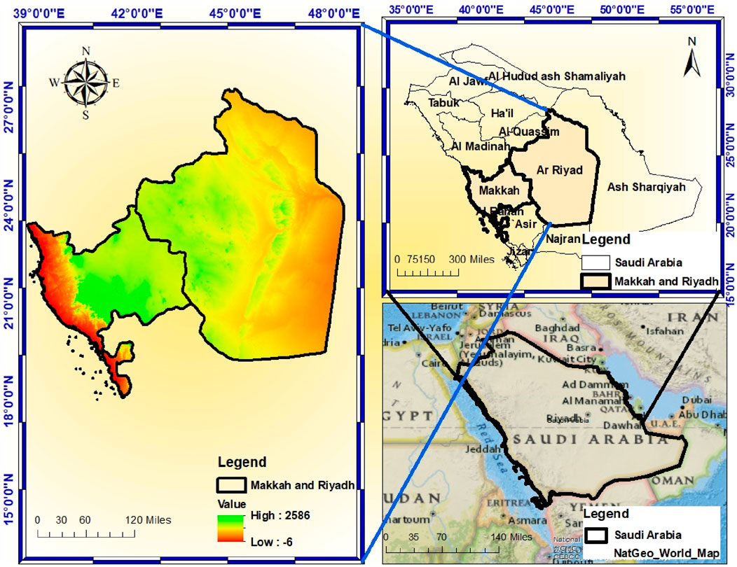
Figure 1. Map of Makkah and Riyadh highlighting the study area.

2.2 Data acquisition

In this study, IDF curves were developed for Makkah and Riyadh based on observed and SSPs scenarios using annual precipitation data.

2.2.1 Rainfall dataset overview

Annual rainfall data spanning from 1950 to 2020 visualized in Figures 2, 3 for Makkah and Riyadh were collected from the Climate Knowledge Portal to develop IDF curves. The combination of Makkah’s coastal climate and Riyadh’s inland desert conditions provides a diverse setting for analyzing rainfall variability.

Figure 2

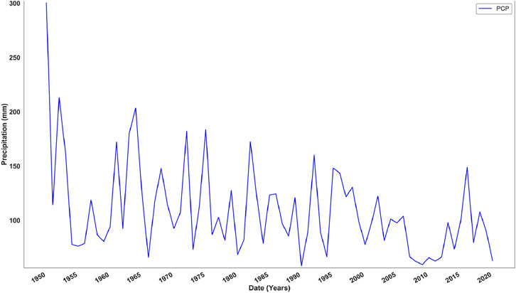
Figure 2. Representation of observed annual precipitation from 1950 to 2020 of Makkah.

Figure 3

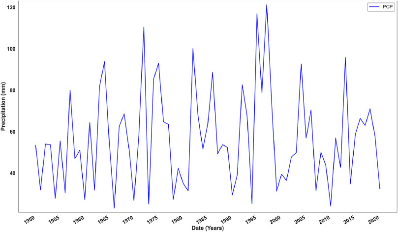
Figure 3. Representation of observed annual precipitation from 1950 to 2020 of Riyadh.

2.3 Downscaling and bias correction

In the context of GCM-based modeling, preprocessing steps such as downscaling and bias correction are indispensable for ensuring that coarse-resolution climate model outputs are consistent with observed local conditions.

2.3.1 Downscaling

Downscaling is a climate science technique used to transform the coarse-resolution data from GCMs into higher-resolution data that more accurately reflects local or regional climate conditions (Teutschbein et al., 2011). GCMs simulate the Earth’s climate system at a global level, typically with spatial resolutions between 100 and 300 km (Palmer, 2014; Ullah et al., 2023). While these models capture broad climate patterns effectively, their coarse resolution makes them less suitable for localized studies, such as evaluating climate change impacts on specific regions, cities, or watersheds (Humphries et al., 2024). To overcome this limitation, the raw GCM data, which is often at a coarse spatial resolution, was downscaled to match the local scale of Makkah, making the data more appropriate for regional climate impact assessments. In this study, a Python script was developed to implement the downscaling process for GCM data, specifically focusing on extracting and processing precipitation data for the study area. The script utilizes the xarray and pandas libraries to handle NetCDF files, the standard format for storing climate data. The primary function of the script, extract_gcm_data_to_excel, is designed to extract precipitation data for specific geographic coordinates from the GCM file, convert the units from kilograms per square meter per second (kg/m²/s) to millimeters per day (mm/day), and save the processed data into an Excel file for further analysis. The script begins by iterating through all NetCDF files in a specified folder, identifying the precipitation variable within each file. It then extracts data for the nearest latitude and longitude coordinates provided by the user, ensuring alignment with the study area. A critical step in the process is the conversion of precipitation units from kg/m²/s to mm/day, achieved by multiplying the values by 86,400 (the number of seconds in a day). This conversion is essential for making the GCM data compatible with hydrological analyses and IDF curve development. The extracted data is then compiled into a single pandas DataFrame. Finally, the downscaled data is saved into an Excel file, providing a structured and accessible format for subsequent analysis. This script plays a crucial role in the downscaling process by enabling the extraction and preprocessing of GCM data at a local scale, ensuring its suitability for evaluating future climate scenarios and their impacts on extreme precipitation events in the study area.

2.3.2 Bias correction

Bias correction is a method used to rectify systematic errors in climate model outputs, hydrological models, or remote sensing data (Shrestha et al., 2017). Climate models frequently diverge from observed data due to limitations in resolution, parameterization, or initial conditions (Randall et al., 2007). By adjusting the model’s statistical properties to better align with observed data, bias correction enhances the accuracy of the model’s predictions. One of the most powerful techniques for quantile mapping. In this study, a Python script was developed to apply Quantile Mapping (QM) bias correction to GCM precipitation data. The script loads historical GCM data, observed data, and future GCM projections under SSP245 and SSP585 climate scenarios from Excel files. These datasets are processed to ensure alignment based on the “Date” and precipitation columns. The script calculates percentiles for observed and historical GCM data, and then maps GCM values to observed quantiles, ensuring statistical consistency. The correction function is applied to both historical and future GCM data, maintaining consistency across different periods and scenarios. The corrected data is saved in Excel format for further analysis. This ensures the corrected GCM data is suitable for IDF curve development and climate impact assessments.

2.4 Simulated climate data from GCMs

To evaluate future climate trends, five GCM models, selected based on their strong performance in simulating precipitation in arid regions recommended by different literature (Sharif, 2015; Alotaibi et al., 2018; Hassan et al., 2016), were downloaded from the CMIP6 portal. These models are presented in Table 1.

Table 1

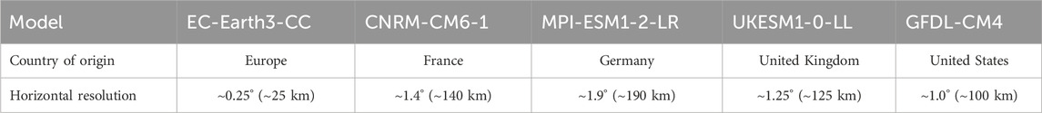
Table 1. GCM Models used in this research.

These models were chosen for their reliability in forecasting climate parameters in the Arabian Peninsula, enabling a thorough analysis of potential future climate changes in both Makkah and Riyadh.

3 Methodology

To develop the IDF curve for two stations, Makkah and Riyadh, using five different GCM models under two SSPs, SSP245 and SSP585, after downscaling and bias correction, and then perform multi-modeling using machine learning. Firstly, the five GCM models were downscaled and bias-corrected using linear scaling techniques. Subsequently, feature engineering was conducted using CatBoost and LightGBM to select the best combination of bias-corrected GCMs that closely resemble observed data. Secondly, an MME was computed for the top three GCMs for precipitation using the XGBoost technique. Thirdly, three various distributions were chosen: Gumbel, Log-Pearson 3, and Gamma distributions. The former distributions were the basis in constructing the IDF curves of observed and future precipitation data across two distinct SSP scenarios (SSP245 and SSP585) of CMIP6 (see Figure 5).

3.1 Refining GCM rainfall with downscaling and bias correction

A downscaling involves the practice of converting the coarse spatial resolution of GCMs to finer resolutions, more appropriate for local and regional studies (Ullah et al., 2023). This allows the development of fine-scale forecasts of weather phenomena, including rainfall, on finer spatial resolutions, with more accessible results at local levels. Where Bias correction on the other hand is the process of modifying the output of GCMs to handle systematic mistakes or bias within the model predictions.

In this study, the bias correction algorithm was carried out in the linear scaling technique, as it is associated with ease of implementation and computing efficiency. It is a method of ensuring biases are adjusted but retaining the patterns and variability in the original GCM. To ease this process, a Python code was constructed and was applied to downscale, and bias correct the data of the GCMs (Haider et al., 2020).The whole process of bias correction is indicated in Figure 4. Adopting an ensemble approach after bias correction is a strong suggestion as proposed by Teutschbein and Seibert (Teutschbein and Seibert, 2012) where the results of several bias-corrected climate projections are used to enhance the credibility and reliability of the climatic projections.

Figure 4

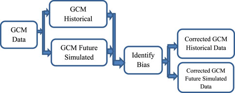
Figure 4. Bias correction technique applied in this study.

Figure 5

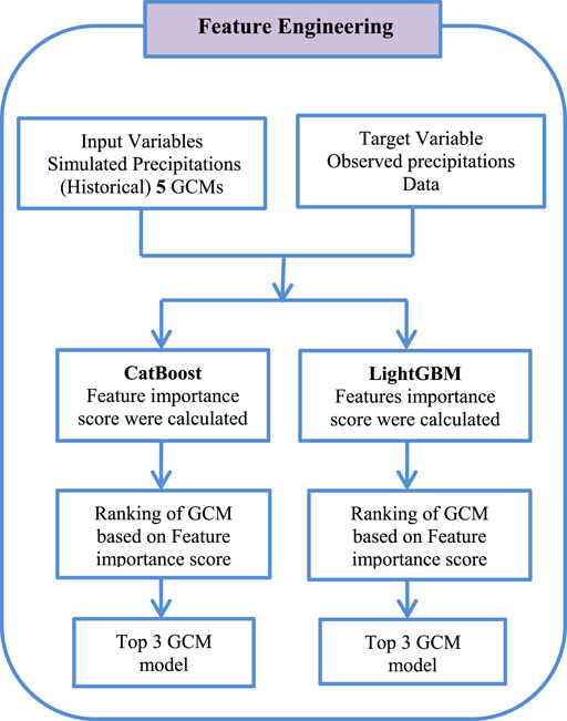
Figure 5. Flowchart of the feature engineering process.

3.2 Multi-Model Ensemble approach (MME)

There is an overall approach that has been used by several climate science researchers and applied hydrologists known as method of MME where the projections of several general circulation models are combined to improve the accuracy and stability of climate projections (Anwar et al., 2024). GCMs are numerical models that simulate the entire climate system on the surface of the earth, by discretizing numerical solutions of physical equations that represent atmosphere, oceans, land, and ice.

In this research, MME process was introduced after feature engineering to identify the most important GCMs. CatBoost, and LightGBM, two of the most advanced Machine learning classifiers were then used to calculate feature importance scores. GCMs with the maximum values of such scores were kept overcoming redundancy and improve the reliability of the ensemble. Three disparate Machine learning methods, which include the AdaBoost framework, CatBoost, and the XGBoost, were assessed versus the chosen GCMs to construct the MME. The created forecasts were synthesized through procedures of ensemble averaging, thus capitalizing on the complementary capabilities of the member models and increasing the forecast accuracy and repeatability, and at the same time highlighting the extraordinary roles played by the highest-rank GCMs. The combination of feature selection and an ensemble model, therefore, produced sound, comprehensible results, hence proving the usefulness of this framework when dealing with the issues of climate and hydrological modeling.

3.3 Feature engineering

In predictive modeling, the process of designing, transforming, or creating the input features (variables) to optimize the performance of the Machine learning models is termed feature engineering. Gradient-boosting models have become well-established techniques commonly used to this end, which include the CatBoost and LightGBM libraries, whose advantageous properties comprise efficient speed, scalability, and productive predictive ability. One of the most prominent characteristics of the two systems is the ability to give a feature-importance score that measures the contribution of every variable to the predictive capacity of the model. The scores are essential in terms of determining the most influential points of learning with datasets as an effective feature selection, or model interpretability, and consequent optimization.

3.3.1 Categorical Boosting (CatBoost)

CatBoost is a more advanced version of gradient boosting with its application in tasks such as classification as well as regression. It minimizes the difference between the predicted and observed values in cases of regression using numerous loss functions, such as Huber Loss or Quantile Loss (Hancock and Khoshgoftaar, 2020). Peculiarity of CatBoost is that it allows working with the categorical variables, avoiding heavy preprocessing; this feature makes the algorithm especially beneficial to work with the data allowed to have both numerical and categorical components. CatBoost reduces overfitting by integrating ordered boosting, which results in creation of efficient and accurate predictions.

To use CatBoost in regression, the output results in continuous numeric values, making the tool applicable in price prediction, demand forecasting, and energy consumption estimation. The framework requires very few parameters to tune and can be implemented on a CPU or GPU, which provides both scalability with large finite datasets as well as efficiency. The integrated interpretability mechanisms that the algorithm has implemented, including feature importance scores and SHAP values, enable the algorithm not only to achieve high predictive accuracy but also to give pertinent insight into what contributes to the given prediction.

In this application, the Python script allows the use of CatBoost in obtaining the scores of feature importance. It first imports such modules as pandas and numpy to manipulate the data, scikit-learn to select the model and process missing values, CatBoostRegressor to use in the Machine learning model, and matplotlib to visualize the data. The dataset, contained in an excel file, is loaded at a desired file location with the help of pandas and then the features and the target variable are then separated. Training of CatBoostRegressor model occurs using an imputed training data, pre-decided learning rate, number of iterations, and depth. The scores of feature importance are acquired with the help of the get_feature_importance method. These scores are followed by normalization of scores to [0, 1] interval to compare them directly with other models.

3.3.2 Light Gradient Boosting Machine (LightGBM)

LightGBM is an effective ML framework that possesses high efficiency, scalability, and speed, especially on larger datasets (Zhang et al., 2019). Unlike the other methods of gradient boosting which formed trees in a level-wise manner, light GBM uses a leaf-wise method to grow by having the computational resources focused on the leaves that pose the greatest contribution to the reduction of the loss. This of experimentation results in an efficient model with fewer trees but a more powerful model that is inherently prone to over extrapolation when used on a medium-sized dataset.

A Python code of LightGBM was designed in the current research to estimate feature importance scores. The script imports the required libraries at the beginning of the code such as the pandas library and numpy library, to manipulate the data, the scikit-learn library, to select the model and deal with the missing values, the LightGBM library, the machine learning model used, and the matplotlib library to visualize the data. Pandas is used to load the dataset, which is available in an Excel file in each file path. The features and target variable are then separated. The LightGBM Regressor model is then trained on the imputed training data with a specified learning rate, number of estimators, and maximum depth. The feature importance scores are retrieved from the feature importances_ attribute. These scores are then normalized to a [0, 1] scale to allow for direct comparison with other models.

3.4 Machine learning models

After the top three GCM models were chosen based on feature engineering, as indicated in Figure 6, three machine learning models were trained on them to ensemble future climate data.

Figure 6

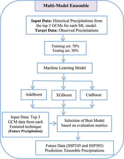
Figure 6. Flowchart of machine learning models.

3.4.1 Adaptive boosting (AdaBoost)

AdaBoost is an ensemble learning algorithm designed to improve the performance of weak learners, typically decision stumps (one-level decision trees), by combining them into a strong model (Wu and Zhao, 2010). The algorithm works iteratively, training each weak learner on the dataset while adjusting the weights of the data points. Initially, all data points are given equal weights. However, after each iteration, misclassified points are assigned higher weights, forcing subsequent learners to focus on the harder-to-classify instances. Each learner is assigned a performance-based weight, and the final model combines all weak learners’ predictions using a weighted majority vote.

In this study, Python code was developed to implement the AdaBoost model. Initially, the essential libraries include pandas for data manipulation, scikit-learn for model development and evaluation, and SciPy. Stats for hyperparameter tuning were imported. The dataset was loaded from an Excel file, and the input features were extracted from the top three GCM models, while the target variable was the observed precipitation. The dataset was then split into training and testing sets, with 30% of the data reserved for testing. A DecisionTreeRegressor with a maximum depth of 5 was chosen as the base learner for the AdaBoost model. An AdaBoost regressor was built, and grid search was performed through RandomizedSearchCV to find the best hyperparameters: the number of estimators (n_estimator), the learning rate, and the random state. The model was then trained after identifying optimal settings and tested against the training and testing datasets. The performance measures, i.e., R², Mean Squared Error (MAE), and Mean Absolute Error (MSE) were then used to estimate the model precision and predictive capacity.

3.4.2 Extreme Gradient Boosting (XGBoost)

XGBoost is a recent and efficient gradient-boosting learning framework specifically created to work on structured and tabular data and to deal with regression and classification problems. XGBoost has been designed to be effective in hydrological modeling due to its ability to model nonlinear data, sparseness and extreme data points (Chen and Guestrin, 2016; Mosavi et al., 2018). These strengths allowed our study to surpass other ensemble techniques, which is why it is especially beneficial in precipitation modeling in arid and semi-arid conditions with limited and highly variable data (Mosavi et al., 2018). The XGBoost algorithm is generally recognized in terms of speed, accuracy and scalability, thus, making a favorite choice in the competitive system of machine-learning and even in large-scale practices. Some of its main advantages are regularization algorithms like L1 and L2 that are intended to address overfitting, management of missing values, parallelization support, and memory-optimizing techniques.

The current study is based on the creation of the Python code to apply to the XGBoost model. The essential libraries, “pandas”, “scikit-learn” to evaluate models, and “xgboost”, to use a model, and “scipy.stats” to tune parameters, were imported first. A data acquired in excel form contained the input characteristics, which refer to the best three Global Climate Models, as well as the observed precipitation as the focus variable. This data was then divided into training and testing data with 30% of it being the latter. A model was built using XGBoost regressor and hyperparameters tuning was performed using “RandomizedSearchCV” by optimizing hyperparameters like number of estimators (“n_estimator”), learning rate, maximum tree depth (“max_depth”), random state. Once the best set of parameters was found, the model was trained with the help of the training dataset and was evaluated with the help of both training and testing sets. The most significant performance measurements, i.e., R², MAE, and MSE were used to assess the accuracy and predictive ability of the model, hence, guaranteeing optimal and reasonable estimation of observed precipitation data.

3.4.3 Categorical Boosting (CatBoost)

The current study assessed the performance of CatBoost, a high-performance gradient-boosting framework designed by Yandex and fine-tuned in terms of handling categorical variables. This algorithm makes the workflows easier and reduces the risk of overfitting that appears in the consequences of poor encoding. Additional features are strong missing values treatment, extensive cross-validation, and support of GPU acceleration, which makes CatBoost applicable to a wide range of tasks, both in terms of small and large datasets. By implementing optimization methods of superior quality, the algorithm has displayed exceptional predictive precision, but at the same time, controlled overfitting, returning trusted results in the regression and classification tasks.

The experimental setting of the CatBoost in a Python-based environment was performed by installing necessary libraries: pandas to work with data, scikit-learn to divide the dataset and evaluate the performance, CatBoost to create a model, and scipy. stats to optimize hyperparameters. It included information on input features based on the three leading climate models worldwide, the observed precipitation as the target variable, using the dataset, which was obtained through an Excel file. The data was split up, where 30% of the data was used in testing. The key ML model was a “CatBoostRegressor” due to its ability to work with categorical data even when there are no such data in the analysis. Hyperparameter optimization was performed using the “RandomizedSearchCV” routine and maximized the iterations, learning rate, the depth of the trees, and the random seed. Once the best parameterization was found the final model was then trained on the complete dataset.

3.5 Machine learning model evaluation criteria

R², MSE, and MAE were three statistical parameters used to measure the performance of Machine learning models in the current research. These metrics, in combination, are a valuable representation of how accurate and precise the models are when they make predictions (Ullah et al., 2023).

3.5.1 Mean squared error (MSE)

A commonly used derived metric to evaluate regression models’ performance is called mean squared error (MSE). It is the arithmetic mean of squared residuals or the difference between predicted and observed outcomes. The suitable formula of computation is presented in Equation 1:

$MSE=\frac{1}{n}{\displaystyle \sum _{i=1}^n}{\left(y_i-\overline{y_i}\right)}^2(1)$

3.5.2 Mean absolute error (MAE)

MAE is the average variation between the observed values and the predicted values in the dataset (Schneider et al., 2022). MAE can be computed by Equation 2.

$MAE=\frac{1}{n}{\displaystyle \sum _{i=1}^n}\left|y_i-\overline{y_i}\right|(2)$

3.5.3 Coefficient of determination (R²)

R² is a statistical measure that represents the proportion of the variance in the dependent variable that is explained by the independent variables in a regression model. It is calculated using Equation 3.

$R^2=\frac{{\left({\displaystyle {\sum }_{i=1}^n}\left(y_i-\overline{y}\right)\left(y_i^1-\overline{y^{\prime }}\right)\right)}^2}{{\displaystyle {\sum }_{i=1}^n}{\left(y_i-\overline{y}\right)}^2{\sum }_{i=1}{\left(y_i^{\prime }-\overline{y^{\prime }}\right)}^2}(3)$

where:

y_i = observed values,

y′ = predicted values,

$\overline{\mathrm{y}}$ = mean of observed values,

n = number of data points.

These statistical indicators are commonly utilized by researchers to evaluate the model’s accuracy and determine its suitability for a specific task or dataset.

3.6 Development of IDF curves

In hydrology, the trend of constructing IDF curves forms an imperative product in the analysis of the interdependence of the rainfall intensity, period, and recurrence interval. These curves act as statistical identifications of rainfall patterns over different periods of time, thus assisting the development of efficient drainage structures and flood hazard management. The process begins by putting up long-term records of rainfall at local weather stations, which is then followed by calculating the rainfall intensities at sequential time intervals ranging from a few minutes to hours. This set of data is then strictly examined to ascertain the IDF relationship, traditionally represented graphically in intensities of rainfall against duration at a specific recurrence interval. The generation of IDF curves is normally in form of a systematic three-step approach that has been recalibrated with discrete time periods: 5, 10 min, and up to 1,440 min based on probability distribution functions to correspond with the observed data so as to determine rainfall intensities in terms of a given return period of 2, 10, 25, 50, 75 and 100 years. Being an inevitable tool in water-resource development, IDF curves are used to design stormwater management units and facilities.

Rainfall data collected are often fitted to a probability distribution, usually the Gumbel distribution, to find rainfall intensities of different return periods with widely different separation. The statistical tests are used to determine the accuracy and reliability of the derived IDF curve. Rapid changes of rainfall regimes caused by climatic change can require IDF curve recalibrations to adjust to changing patterns. IDF curves play an important role in urban planning, flood management, and infrastructure development, owing to their ability to provide information related to the severity and the frequency of the precipitation events, which directly affects the design of the stormwater drainage systems, flood management and overall water management efforts.

3.6.1 Empirical reduction equation for short-duration rainfall estimation

The empirical reduction equation is one of the broadly used tools in hydrological studies to predict the intensity of rainfall in shorter periods using long-term duration data. The Indian Meteorological Department (IMD) has recommended one of the simplest equations (Kawara and Elsebaie, 2022):

$P_t=P_{24}\sqrt[3]{\frac{t}{1440}}(4)$

The corresponding Equation 4 gives the short-duration intensity, P_t, after scaling a 24-h intensity, P₂₄, by dividing the certain time, t. It is particularly applicable in arid regions such as Saudi Arabia where high resolution data is not available; however short-duration estimations are required to construct IDF curves and to assess the risk of floods within urban regions.

3.6.2 Probability distribution fitting

The frequency distribution method of fitting the Probability Density Function (PDF) involves the application of an adequate theoretical distribution to empirical data to determine the probability of different results yielded by a random variable. The process is widely used in hydrological analysis, especially in parameters estimation of rainfall or streamflow in the sense that it aims at determining distribution that best resembles the observed data. Numerous theoretical distributions are in common usages in different parts of the globe, some examples outlined here under are the Gumbel Distribution, the Gumbel Distribution (Extreme Value Distribution 1), the Normal Distribution, the Log-Normal Distribution, the Pearson Distribution, and the Log Pearson 3 Distribution. Three of the most used PDFs in appliance and practices in hydrology and statistics, and in this case, attention given to modeling extreme events: Log-Pearson 3, Gumbel Distribution (Extreme Value I) and Gamma Distribution. All these distributions consist of their unique benefits based on the data that is to be analyzed. The Log-Pearson 3 distribution has evolved to a common standard in analysis with flood frequencies in that: it can model adequately the skew common to many hydrological records rainfall and streamflow, and it is particularly evident when the data has a large right tail. As a result, the capacity of its skewness explains the Log-Pearson 3 is invaluable in the modeling of hydrological extremes that are not normal. The Gumbel Distribution (Extreme Value I) is highly suitable towards analysis of the highest or the lowest value of a dataset, e.g., the peak rain-fall events or largest stream-flow events and as such a foundation of extreme value theory. Subsequently, it is commonly utilized in the evaluation of flood risk and storm water management mechanisms to calculate likelihood as well as estimated recurrence instances of extreme precipitation events. The Gamma distribution has a very flexible shape that makes it regularly used on a continuous positive variable such as rainfall intensity and streamflow. This property, which allows it to approximate both light- and heavy-tailed distributions conveniently, qualifies it to be used to model phenomena that occur in bursts, e.g., storms. The distributions present a powerful analytical package to hydrologic modelling, with which a researcher or an engineer can study and predict extreme events about water resource management and design of infrastructure systems, as well as the insights generated regarding climatic-induced effects.

4 Log-Pearson 3 distribution

The Log-Pearson 3 distribution is a pivotal statistical parameter in applied hydrology, especially in modelling data that is positively skewed, which is revealed in the magnitudes of floods, rainfall intensity, as well as streamflow records. Its usefulness is in managing the situations in which the cumulative distribution becomes extremely right skewed, which is also a common behavior of extreme hydrological phenomena like floods.

The implementation of this distribution is covered by the results of the transformation of the original data to the logarithmic axis, resulting in an asymmetric normal distribution. This mapping makes the model applicable even with the datasets that cannot be appropriately modelled by the conventional normal distribution. In combining consideration of the mean and the tails of the distribution at the same time, the Log-Pearson 3 model can represent a natural asymmetry in distributions of natural phenomena like the amounts of rainfall and floods. This allocation, therefore, is part of the management of flood risks, not to mention the design and establishment of strong water management systems.

4.1 Calculation methodology

The rainfall data is first converted to logarithmic values using Equation 5.

$Pricipitation={\log }_{10}\left(OriginalPricipitation\right)(5)$

Then the annual precipitation is initially reduced using Equation 6.

$P_t=P_{24}{\left(\frac{t}{1440}\right)}^{\frac{1}{3}}(6)$

Where P₂₄ is the 24-h precipitation, and t is the duration (in minutes). Next, the mean, standard deviation, and skewness are calculated. Then the cumulative probability P is determined using Equation 7.

$P=1-\frac{1}{T}(7)$

where T is the return period (in years). Then the frequency factor K_t is calculated using Equation 8.

$K_t=Z+\frac{Skewness}{6}\left(Z^2-1\right)(8)$

where Z value is computed using the formula Equation 9:

$Z=\text{NORMSINV\hspace{0.17em}}\left(P\right)(9)$

Finally, the precipitation for a given time (T) and duration (t) is calculated using Equation 10.

$P_t=\mu +K_{t}S(10)$

where

μ = arithmetic mean of the rainfall records,

S = standard deviation,

K_t = frequency factor, calculated as described above.

Finally, convert the precipitation estimate back to its original scale using Equation 11

$P={10}^{P_t}(11)$

To facilitate the development of IDF calculations for precipitation and rainfall intensity (I in mm/hr), the formula is given by Equation 12.

$I=\frac{{\mathrm{P}}_{\mathrm{t}}}{\mathrm{t}}(12)$

where

I is the rainfall intensity in mm/h, P_t is the extreme rainfall value for the given duration and t is the duration in hours.

This framework provides an effective method for determining precipitation estimates for various durations and return periods, forming the basis for hydrological design and analysis.

5 Gumbel Distribution (extreme value I)

In hydrology, the Gumbel distribution serves as the Extreme Value I distribution, and it has generally been used to describe the record or record minimum of meteorological or hydrological variables, such as extreme rain events, peak flood levels and high wind velocity. The extreme value theory centers on this distribution, and it is applicable to analyses of the largest or smallest observations in a sample, called peak over-threshold extremes. The Gumbel distribution assumes that the extreme values (e.g., maximum annual rainfall or peak river discharge) follow a specific pattern and can be modeled with two parameters: the location parameter (which shifts the distribution) and the scale parameter (which defines the spread of the distribution). This makes it valuable for predicting extreme events and estimating their return periods.

Stepwise Procedure for IDF Curve Construction Using the Gumbel Distribution

1. Convert Annual Precipitation Data for Corresponding Durations: Convert the annual precipitation data for the corresponding durations using equation (VI) to transform the precipitation data into the desired duration.

2. Compute Statistical Measures: Compute the mean (μ) and standard deviation (S) of the transformed precipitation data for each duration. These statistical measures help in understanding the central tendency and the spread of the rainfall data.

3. Determine the Exceedance Probability (P): The exceedance probability P for a return period T is calculated using the following Equation 7.

4. Calculate the Frequency Factor (K_t​) Using the Gumbel Distribution: The frequency factor K_t is computed using the Gumbel distribution formula. As given by Equation 13.

$K_t=\left\{-\ln \left[-\ln \left[P\right]\right]\right\}(13)$

where

P is the exceedance probability and K_t represents the scaling factor for the rainfall intensity corresponding to the return period.

5. Compute Extreme Rainfall Values for Different Durations: Using the calculated mean (μ), standard deviation (S), and frequency factor (K_t), the extreme rainfall values for a specific return period and duration are determined using Equation 10.

6. Repeat for Different Return Periods: The steps above are repeated for different return periods, such as 2 years, 10 years, 25 years, 50 years, 75 years, and 100 years, to calculate the corresponding extreme rainfall values for each duration.

7. Calculate Rainfall Intensity (I) for Each Duration: To facilitate the development of IDF calculations for precipitation and rainfall intensity (I in mm/hr), the formula is given by Equation 12.

The current methodological framework outlines a process of developing an intensity-duration-frequency (IDF) curve using the Gumbel distribution, hence probabilistically providing information related to the expected rainfall intensities associated with the defined return periods and durations.

6 Gamma Distribution

Gamma distribution is a popular statistical model of continuous positive data used in hydrology, engineering and statistics, especially measurements of rainfall, streamflow and quantities of precipitation. This distribution is well deemed in capturing heavy-tailed property, i.e., burst behavior which happens in a storm situation, and it is used around the world. The distribution is parameterized in terms of a shape parameter k and a scale parameter θ, providing the flexibility of the distribution tail: the heaviness or lightness of the tails depends on k, and the spread depends on θ. The Gamma distribution is therefore a flexible model which can be used in a wide range of applications such as hydrological modelling, survival analysis and time-to-event data analysis. All the other formulas are the same as for the Gumbel distribution, except for K_t. To calculate the K_t frequency factor for a Gamma distribution, follow these steps:

All the other formulas are the same as for the Gumbel distribution, except for K_t. To calculate the K_t frequency factor for a Gamma distribution Equation 14 can be used.

$K_t=Xp-\frac{Mean}{StandardDeviation}(14)$

The next step is to use the inverse CDF of the Gamma distribution to find the precipitation amount X_P corresponding to P. In Excel, it can use the GAMMA.INV function for this. As given by Equation 15.

$X_P=\text{GAMMA}.\text{INV}\left(P,k,\mathrm{\theta }\right)(15)$

where

P is the non-exceedance probability,

k is the shape parameter of the Gamma distribution,

θ is the scale parameter of the Gamma distribution,

X_P is the precipitation amount corresponding to P.

This process computes the K_t frequency factor for the Gamma distribution, which represents how the precipitation amount deviates from the mean, scaled by the standard deviation.

7 Results and discussion

7.1 Evaluation of feature engineering

Feature importance scores were calculated using CatBoost and LightGBM. These scores are invaluable for identifying the most influential features in a dataset, aiding in feature selection, model interpretability, and optimization.

7.1.1 Selection of GCM via of CatBoost

The feature importance was calculated using CatBoost conducted of various GCM models. For Makkah, the normalized CatBoost feature importance scores were as follows: MPI-ESM1-2-LR (0.2542), CNRM-CM6-1 (0.2382), EC-Earth3-CC (Europe) (0.2004), GFDL-ESM4 (0.1970) and UKESM1-0-LL (0.1102). For Riyadh, the normalized CatBoost feature importance scores were EC-Earth3-CC (Europe) (0.2489), GFDL-ESM4 (0.2199), MPI-ESM1-2-LR (0.2124), UKESM1-0-LL (0.1597), and CNRM-CM6-1 (0.1590). then the top 3 GCM models for each station is taken as input variables. These scores provide insight into the relative significance of each model in contributing to the overall prediction for each location.

7.1.2 Selection of GCM via LightGBM

Similarly, feature importance scores were calculated using LightGBM for Riyadh and Makkah. For Makkah, the normalized LightGBM feature importance scores were: MPI-ESM1-2-LR (0.4400), CNRM-CM6-1 (0.3140), GFDL-ESM4 (0.2260), EC-Earth3-CC (Europe) (0.0120), and UKESM1-0-LL (0.0080). For Riyadh, the normalized LightGBM feature importance scores were: UKESM1-0-LL (0.6040), GFDL-ESM4 (0.1620), EC-Earth3-CC (Europe) (0.0980), MPI-ESM1-2-LR (0.0960), and CNRM-CM6-1 (0.0400). The performance assessment of GCM-guided predictive framework shows the unequal evidential capacity of the constituent members of the LightGBM ensembles to both Makkah and Riyadh. The Feature importance metric was referred to isolate the models with the greatest contribution in each city. Based on this criterion we selected models which showed in both LightGBM and CatBoost computation: MPI-ESM1-2-LR, CNRM-CM6-1 and GFDL-ESM4 belong in the high tier of Makkah ranking, and GFDL-ESM4, EC-Earth3-CC (Europe) and UKESM1-0-LL in the top of Riyadh.

Two complementary charts, the radial bar charts and radar, were used to visualise the relative importance of the models used. As shown in Figures 7, 8, the most significant impact on rainfall patterns of Makkah is imposed by the MPI-ESM1-2-LR model, but in Riyadh the GFDL-ESM4 model performs a similar role. Radar graphs also show the multidimensional contribution of each model to different predictive variables. These observations can and do align with the results of single-model analyses, which highlight that the explanatory power of a model is situation-specific and may differ quite considerably across geographical location. These findings explain why it is important to take into account spatial variability as a method of determining the model performance and identifying the most appropriate models to use in the evaluation of the effects of regional climate.

Figure 7

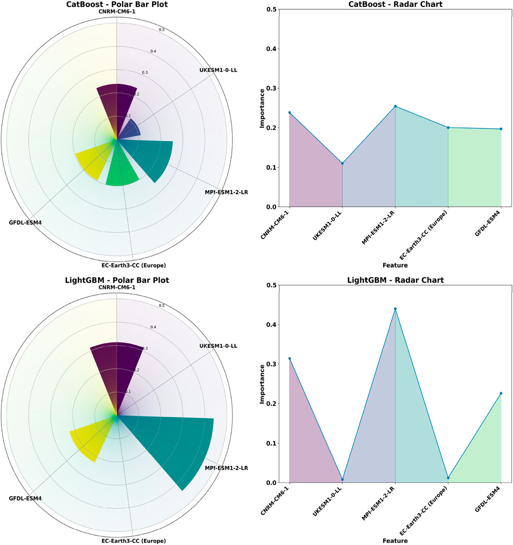
Figure 7. Presents a Radar Chart and a Polar Bar Chart, highlighting the importance of each GCM model for Makka.

Figure 8

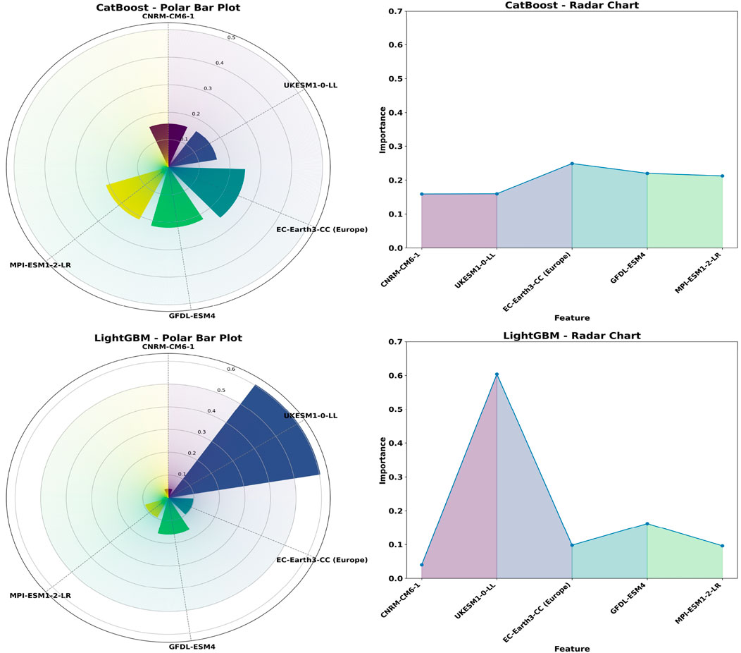
Figure 8. Presents a Radar Chart and a Polar Bar Chart, highlighting the importance of each GCM model for Riyadh.

7.2 Analyzing the effectiveness of the machine learning model

In this study, we used the Multivariate-Moving-Ensemble (MME) framework that utilized three s of statistical learning algorithms, namely, AdaBoost, XGBoost, and CatBoost, to identify the spatially distributed precipitation. The target data were results of precipitation measurements in the global gridded precipitation dataset GPCC version 7.0, whereas the predictors, precipitation forecasts of the top three GCMs of each MME ensemble, were utilized. Data was divided into the training-test stratum of 70:30, which also allows a strict analysis of accuracy and the generalization performance of a model. In every station, out-of-sample validation was conducted by comparing the calculated precipitation to the model prediction and the results were measured in terms of root-mean-squared error (RMSE), the mean absolute error (MAE) and coefficient of determination (R²), all of which are reported in Table 2. In both stations, XGBoost ensemble provided better predictions during the training and test periods, which illustrates its overall better performance among all the ensemble members.

Table 2

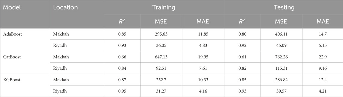
Table 2. Training and testing results of the machine learning models.

Trial 2 added more precipitation forecasts of the best three GCMs which were not used to train the ensembles, and in that way produced forecasts of 5 members of the GCMs. These extended forecasts once again confirmed the strength of XGBoost, which again gave the most successful forecasts, and decisively proved its usefulness in this MME framework in precipitation forecasting.

7.2.1 Evaluation of AdaBoost model performance

A stringent evaluation was adopted to question the capacity of the AdaBoost model in predicting precipitation patterns. The evaluation parameters used in training and testing are performance statistics: R², MAE, and MSE. In the case of Makkah, the model achieved training R² of 0.85 and testing R² of 0.80, MSE values of 295.63 and 406.11, and MAE values of 11.85 and 14.70, respectively, with the best hyperparameter combinations as learning rate of 0.0332, the number of estimators as 66 and random state as 24. The model showed outstanding predictive power in Riyadh with training and testing R² of 0.93 and 0.92, MSE of 36.05 and 45.09, and MAE of 4.83 and 5.15 with hyperparameters `learning rate = 0.5444`, n_estimator = 75 and random state = 73. Even though AdaBoost had good results in both cities, an alternative model was more successful with the provided dataset, which makes AdaBoost an ineffective, less appropriate model. These results, however, demonstrate that the model has a strong predictive power.

7.2.2 Evaluation of CatBoost performance

The CatBoost model has been empirically tested in terms of its usefulness to predict the pattern of precipitation, such that its performance is estimated by the metric criteria R², MAE and MSE, both in training and testing. The model in Riyadh had a great predictive ability with a training R square of 0.84 and a testing R square of 0.82, with MSEs of 92.51 and 115.31 and MAEs of 7.61 and 9.16. The best hyperparameters that were used to generate these results were “depth: 6, iterations: 17, learning rate: 0.1457, and random seed: 54”. In comparison, in the case of Makkah, the model worked average with training R² = 0.66 and testing R² = 0.61, then MSE = 647.13 and 762.26, as well as MAE = 19.95 and 22.90. The best hyperparameters of the Makkah were “depth: 8”, “iterations: 162”, “learning rate: 0.0201” and “random seed: 95”. Where CatBoost demonstrated a strong performance in Riyadh, its comparatively weaker performance in Makkah suggests that perhaps models made with regional data-specificities should be used, since model performance appears to be region-dependent.

7.2.3 Evaluation of XGBoost performance

After developing and thoroughly testing, the XGBoost model has been utilized to predict the patterns of precipitation in Makkah and Riyadh, Saudi Arabia. R², MSE and MAE were determined in terms of the models-performance because of training and testing. The XGBoost model showed high levels of accuracy in Makkah because its R² was 0.87 in training and 0.85 in testing; MSE was 252.70 and 286.82 in training and testing, respectively; and MAE was 10.33 and 12.40 in testing and training, respectively. The best hyperparameters adopted in Makkah were learning rate = 0.0165, max_depth = 18, n_estimator = 110 and random state = 6. In the case of Riyadh, the model produced equally satisfactory results and had R² of 0.95 in training and 0.93 in testing, and MSE of 31.27 and 39.57, and MAE of 4.16 and 4.21. Then the respective hyperparameters are: learning rate = 0.0257, max_depth = 16, n_estimator = 87, and random state = 67.

In both regions, the XGBoost model yielded a better result than its previous versions and other datasets, AdaBoost, and CatBoost, indicating fewer prediction errors, with minimal MSE and MAE values and maximum R² values. These datasets, alongside the literature about the XGBoost performance, could be viewed as a sign of the fact that this model provides trustworthy and stable predictions about rainfall.

XGBoost outperformed the other models, achieving the highest accuracy in both Makkah (R² = 0.85, MAE = 12.40, MSE = 286.82) and Riyadh (R² = 0.93, MAE = 4.21, MSE = 39.57). Its superior performance stems from advanced regularization, shrinkage, and tree-pruning strategies, which reduce overfitting and capture nonlinear rainfall patterns more effectively. In comparison, AdaBoost, though strong in Riyadh (R² = 0.92, MAE = 5.15, MSE = 45.09), was weaker in Makkah (R² = 0.80, MAE = 14.70, MSE = 406.11), reflecting its sensitivity to outliers. CatBoost showed mixed results, performing moderately in Riyadh (R² = 0.82, MAE = 9.16), MSE = 115.31 but poorly in Makkah (R² = 0.61, MAE = 22.90, MSE = 762.26). These results confirm the effectiveness and validity of the XGBoost to forecast precipitation in arid Saudi Arabia.

7.3 Probability density functions fitting

This evaluated precipitation data using the probability distribution: Log-Pearson 3, Gumbel and Gamma which are commonly used in hydrology time series and rare events. The model fittings are shown in Figures 9–14 and indicate that the distributions can capture observed trends and variance of precipitation. Kolmogorov-Smirnov (KS), Anderson-Darling (AD) and Chi-Squared (χ²) tests were used to evaluate the goodness-of-fit of observed and projected precipitation of Riyadh and Makkah. To obtain the most suitable approximation to observed precipitation, Gamma fitted Riyadh (KS = 0.084999, AD = 0.44249, χ² = 4.8925) and Makkah, where Log-Pearson 3 is the least suitable. In the case of projected precipitation under SSP245, Gamma most closely represented Makkah (KS = 0.06334, AD = 0.53223, χ² = 8.3171), closely followed by Gumbel, then Log-Pearson 3 (KS = 0.01819, AD = 0.73554, χ² = 4.3681). In SSP585, Makkah (KS = 0.09657, AD = 0.84556, χ² = 5.8115) and Riyadh (KS = 0.17019, AD = 2.51356, χ² = 6.0739) were best fitted by Log-Pearson 3 and then Gumbel and Gamma, respectively.

Figure 9

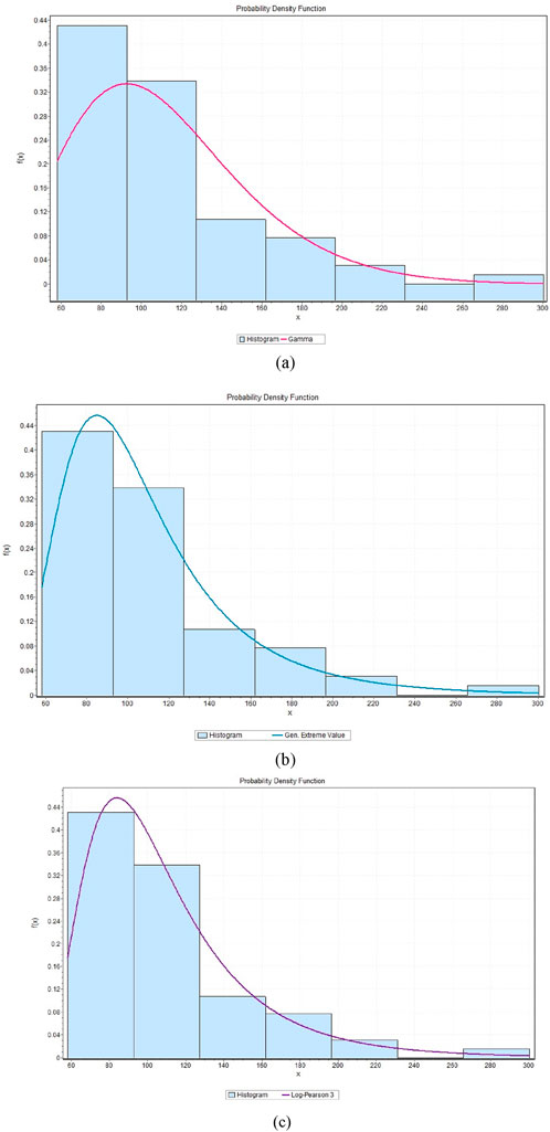
Figure 9. Probability distribution functions of observed precipitation for Makkah, illustrating the (a) Gamma, (b) Gumbel, and (c) Log Pearson 3 distributions.

Figure 10

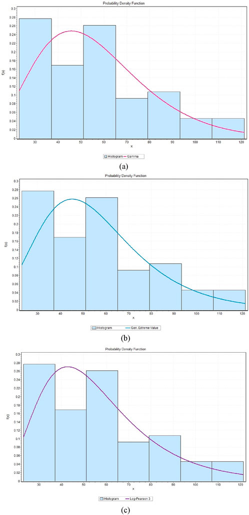
Figure 10. Probability distribution functions of observed precipitation for Riyadh, illustrating the (a) Gamma, (b) Gumbel, and (c) Log Pearson 3 distributions.

Figure 11

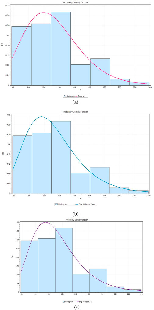
Figure 11. Probability distribution functions of future precipitation under the SSP245 scenario for Makkah, depicting the following distributions: (a) Gamma, (b) Gumbel, and (c) Log Pearson 3.

Figure 12

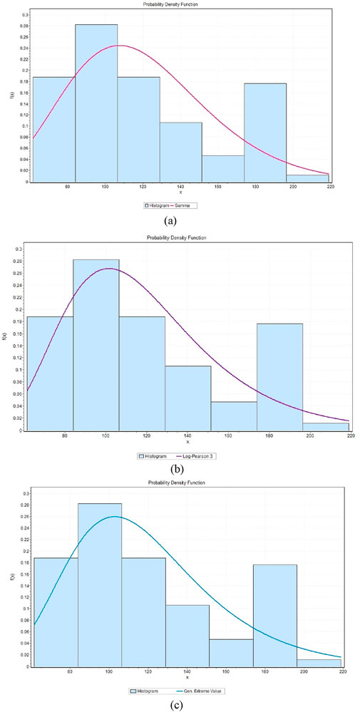
Figure 12. Probability distribution functions of precipitation under the SSP585 scenario for Makkah, showing the following distributions: (a) Gamma, (b) Gumbel, and (c) Log Pearson 3.

Figure 13

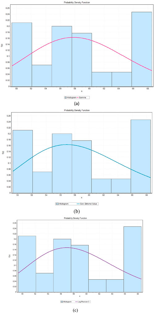
Figure 13. Probability distribution functions of precipitation under the SSP245 scenario for Makkah, illustrating the following distributions: (a) Gamma, (b) Gumbel, and (c) Log Pearson 3.

Figure 14

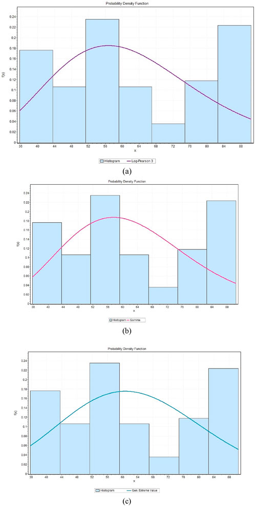
Figure 14. Probability distribution functions of precipitation under the SSP585 scenario for Makkah, depicting the following distributions: (a) Gamma, (b) Gumbel, and (c) Log Pearson 3.

In general, the above analysis indicates that Gamma is best suited to observed data in Makkah under SSP245 and that Log-Pearson 3 gives the best fit in Riyadh and Makkah under SSP585. The results can be used to highlight the importance of the selection of probability distributions in the hydrologic modeling of precipitation extremes.

7.4 Intensity duration frequency curve generation

The IDF curve developed through the selected approach illustrates the relationship between rainfall duration (measured in minutes), intensity (in mm/hr.), and return period (in years). Three different methods have been recommended for calculating rainfall intensity across varying return periods. Figures 15–20 visually represent the correlation between rainfall intensity and duration by integrating these three methods. The correlation between rainfall intensity and duration of storms reveals that short storms yield very high intensities, which drop with extended duration of the storm. It relates how the intensity of rainfall varies with the length of the storms in relation to various return periods. It demonstrates that the intensity of rainfall reduces with time, but over any period of time, the shorter the period, the greater the intensity of the rainfall. This correlation shows the intensity of short and intense storms in comparison with the long and low intensity ones. A notable shift in the return period is evident when the rainfall intensity decreases gradually as the duration extends from 1 to 4 h. The Intensity-Duration Curve demonstrates that the Gumbel method produces the highest intensity values for longer return periods among the three methods.

Figure 15

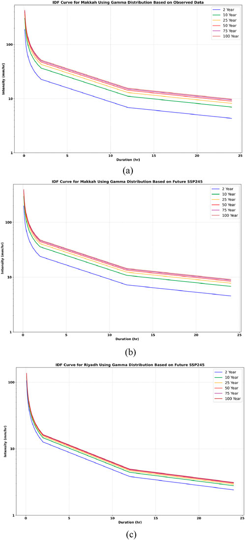
Figure 15. IDF curves for Makkah based on the Gamma distribution, illustrating (a) observed data, (b) SSP245 scenario, and (c) SSP585 scenario.

Figure 16

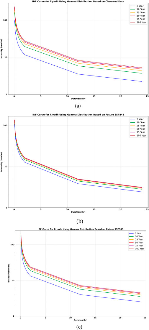
Figure 16. IDF curve for Riyadh using the Gamma distribution, illustrating the following scenarios: (a) observed data, (b) SSP245, and (c) SSP585.

Figure 17

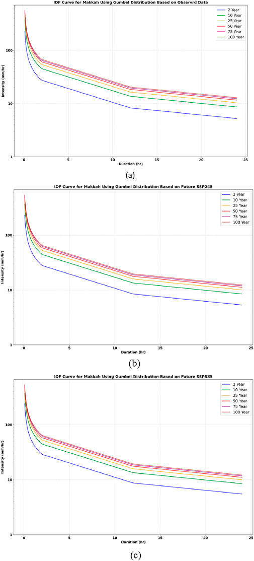
Figure 17. IDF curve for Makkah using the Gumbel distribution, depicting the following scenarios: (a) observed data, (b) SSP245, and (c) SSP585.

Figure 18

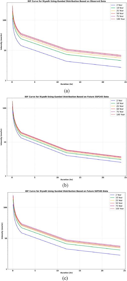
Figure 18. IDF curve for Riyadh using the Gumbel distribution, illustrating the following scenarios: (a) observed data, (b) SSP245, and (c) SSP585.

Figure 19

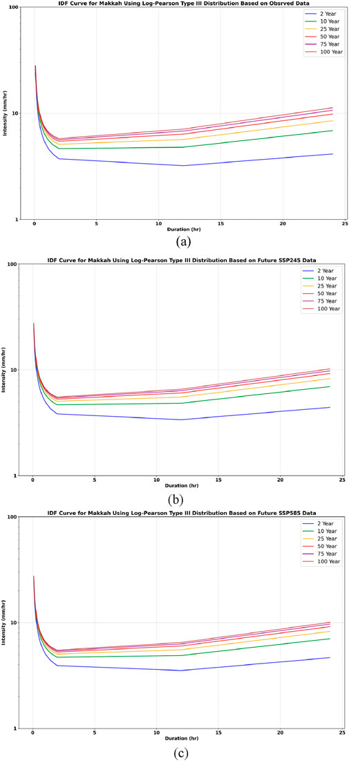
Figure 19. IDF curve for Makkah using the Log Pearson 3 distribution, showing the following scenarios: (a) observed data, (b) SSP245, and (c) SSP585.

Figure 20

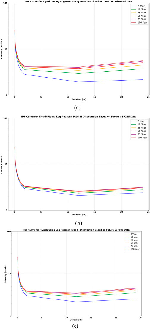
Figure 20. IDF curve for Riyadh using the Log Pearson 3 distribution, depicting the following scenarios: (a) observed data, (b) SSP245, and (c) SSP585.

In both Riyadh and Makkah, it was found that the rainfall intensity under the SSP 585 and SSP 245 scenarios is higher than that of the observed historical rainfall. The intensity follows this order: SSP 585 > SSP 245 > observed rainfall. These findings demonstrate that higher emission scenarios, particularly SSP5-8.5, lead to significant increases in rainfall intensity compared to historical observations and lower emission scenarios such as SSP2-4.5. This evidence obtained demonstrates the importance of incorporating future emission trajectories in climate resilient engineering practice.

8 Conclusions

The current research provides an in-depth analysis of rainfall volatility and future climate scenarios of Makkah and Riyadh using observational records, global climate models (GCMs) and fine Machine learning (ML) methods. In the arid region where Arabian Peninsula is located, precipitation is known to be a vital determining factor to the management of water resources and the development of urban plans. In this regard, the data on annual precipitation recorded between 1950 and 2020 were considered to create individual intensity period-frequency (IDF) curves in each of the cities to describe the existing rainfall pattern and trends. To achieve this goal, five GCMs were, initially, downscaled and bias-corrected through linear scaling strategies. An additional step of feature engineering using the CatBoost and LightGBM allowed determining the GCMs that best approximated the observed precipitation. Three of the GCMs were better, and the MME prediction was calculated on these GCMs, using the XGBoost algorithm to produce highly reliable precipitation predictions. Those three statistical distributions, namely, Gumbel, Log-Pearson 3, and Gamma, were subsequently used to estimate IDF curves of observed precipitation and that of future precipitation projections within the CMIP6 ensemble based on two Shared Socioeconomic Pathways (SSP245 and SSP585), thus making up a comprehensive evaluation of precipitation variability and the future climate trend at the whole of Makkah and Riyadh. It was observed during the analysis that Gamma mostly fits best observed data and Makkah under SSP245 and Log-Pearson 3 is always reliable to fit Riyadh and Makkah under SSP585. Future precipitation scenarios under SSP245 and SSP585 indicated an increase in rainfall intensity, with SSP585 showing the highest intensities. These findings align with existing studies, which confirm that higher emission scenarios, such as SSP585, lead to significant increases in rainfall intensity. The research also explored how emission pathways influence IDF curves. Analysis revealed that as return periods increase, storm durations also increase, while rainfall intensity decreases. Among the statistical methods, the Gumbel distribution produced the highest intensity values for longer return periods. The study formulates a stringent model of predicting future rainfall climates in both Makkah and Riyadh in different climatic conditions. The combination of statistical learning algorithms with ensemble precipitation model-can be applied to other arid and semi-arid areas around the world. For instance, the framework can be adapted to areas in North Africa, the Middle East, and parts of Central Asia, where limited observational data and extreme rainfall events pose similar challenges. As the study combines general circulation model output with applications of Machine learning methods, it confirms the reliability of future climate predictions and provides practical answers to the planning, governance of water resources, and development of infrastructures in coherent cities. The methodology is imperative in enhancing climate resilient and the need to maintain equitable water management in the face of continued climatic change. The results have significant policy implications, especially in the design of infrastructures and water management. The greater prediction of precipitation can be applied to promote resilient storm water drainage systems, improve flood protection standards and train on sustainable water resources approaches in arid and semi-arid areas. The outcomes of the strength models and the bias correction processes also include useful empirical information, which could be utilized in other regions sharing the same climatic characteristics.

Data availability statement

The original contributions presented in the study are included in the article/supplementary material, further inquiries can be directed to the corresponding author.

Author contributions

AB: Conceptualization, Formal Analysis, Funding acquisition, Investigation, Methodology, Software, Writing – original draft. AA: Formal Analysis, Investigation, Methodology, Supervision, Writing – review and editing. AM: Formal Analysis, Investigation, Project administration, Resources, Supervision, Validation, Writing – review and editing. GH: Formal Analysis, Investigation, Methodology, Resources, Visualization, Writing – review and editing. MB: Formal Analysis, Methodology, Validation, Visualization, Writing – review and editing. SH: Formal Analysis, Methodology, Validation, Visualization, Writing – review and editing.

Funding

The author(s) declare that financial support was received for the research and/or publication of this article. Prince Sattam bin Abdulaziz University for funding this research work through the project number (PSAU/2022/01/23530).

Acknowledgments

The authors extend their appreciation to Prince Sattam bin Abdulaziz University for funding this research work through the project number (PSAU/2022/01/23530).

Conflict of interest

The authors declare that the research was conducted in the absence of any commercial or financial relationships that could be construed as a potential conflict of interest.

Generative AI statement

The author(s) declare that no Generative AI was used in the creation of this manuscript.

Any alternative text (alt text) provided alongside figures in this article has been generated by Frontiers with the support of artificial intelligence and reasonable efforts have been made to ensure accuracy, including review by the authors wherever possible. If you identify any issues, please contact us.

Publisher’s note

All claims expressed in this article are solely those of the authors and do not necessarily represent those of their affiliated organizations, or those of the publisher, the editors and the reviewers. Any product that may be evaluated in this article, or claim that may be made by its manufacturer, is not guaranteed or endorsed by the publisher.

References

Agakpe, M. D., Nyatuame, M., and Ampiaw, F. J. H. (2024). Development of intensity–duration–frequency curves using combined rain gauge and remote sense datasets for Weta Traditional Area in Ghana. HydroResearch 7, 109–121. doi:10.1016/j.hydres.2024.01.003

CrossRef Full Text | Google Scholar

Alotaibi, K., Ghumman, A., Haider, H., Ghazaw, Y., and Shafiquzzaman, M. (2018). Future predictions of rainfall and temperature using GCM and ANN for arid regions: a case study for the Qassim Region, Saudi Arabia. Water 10, 1260. doi:10.3390/w10091260

CrossRef Full Text | Google Scholar

Alzahrani, A. S., Abdelbaki, A. M., and Mobarak, B. A. (2024). Exploring the most suitable probability distribution for analyzing annual rainfall data: a case study of Makkah and Jeddah cities. J. Umm Al-Qura Univ. Eng. Archit. 16, 52–63. doi:10.1007/s43995-024-00088-8

CrossRef Full Text | Google Scholar

Anwar, H., Khan, A. U., Ullah, B., Taha, A. T. B., Najeh, T., Badshah, M. U., et al. (2024). Intercomparison of deep learning models in predicting streamflow patterns: insight from CMIP6. Sci. Rep. 14 (1), 17468. doi:10.1038/s41598-024-63989-7

PubMed Abstract | CrossRef Full Text | Google Scholar

Chen, T., and Guestrin, C. (2016). “Xgboost: a scalable tree boosting system,” in Proceedings of the 22nd acm sigkdd international conference on knowledge discovery and data mining, 785–794.

Google Scholar

Doulabian, S., Tousi, E. G., Shadmehri Toosi, A., and Alaghmand, S. J. H. (2023). Non-stationary precipitation frequency estimates for resilient infrastructure design in a changing climate: a case study in Sydney. A Case Study Syd. 10 (6), 117. doi:10.3390/hydrology10060117

CrossRef Full Text | Google Scholar

Dai, C., Qin, X., Zhang, X., Liu, B. J. W., and Extremes, C. (2022). Study of climate change impact on hydro-climatic extremes in the Hanjiang River basin, China, using CORDEX-EAS data. Weather Clim. Extrem. 38, 100509. doi:10.1016/j.wace.2022.100509

CrossRef Full Text | Google Scholar

De Luca, D. L., Ridolfi, E., Russo, F., Moccia, B., and Napolitano, F. J. J. o. H. (2024). Climate change effects on rainfall extreme value distribution: the role of skewness. J. Hydrol. X. 634, 130958. doi:10.1016/j.jhydrol.2024.130958

CrossRef Full Text | Google Scholar

Doost, Z. H., Chowdhury, S., Al‑Areeq, A. M., Tabash, I., Hassan, G., Rahnaward, H., et al. (2024). Development of intensity–duration–frequency curves for Herat, Afghanistan: enhancing flood risk management and implications for infrastructure and safety. Nat. Hazards (Dordr). 120 (14), 12933–12965. doi:10.1007/s11069-024-06730-x

CrossRef Full Text | Google Scholar

Gebrewahid, Y., Eyasu, G., Merasa, E., Abrehe, S., Darcha, G., Manaye, A., et al. (2024). Modeling the ecological niche of rhamnus prinoides L. under climate change scenarios: a MaxEnt modeling approach. Geol. Ecol. Landscapes, 1–17. doi:10.1080/24749508.2024.2433298

CrossRef Full Text | Google Scholar

Gentilucci, M., Rossi, A., Pelagagge, N., Aringoli, D., Barbieri, M., and Pambianchi, G. J. S. (2023). GEV analysis of extreme rainfall: comparing different time intervals to analyse model response in terms of return levels in the study area of central Italy. Sustainability 15 (15), 11656. doi:10.3390/su151511656

CrossRef Full Text | Google Scholar

Haider, H., Zaman, M., Liu, S., Saifullah, M., Usman, M., Chauhdary, J. N., et al. (2020). Appraisal of climate change and its impact on water resources of Pakistan: a case study of Mangla Watershed. Atmos. (Basel). 11 (10), 1071. doi:10.3390/atmos11101071

CrossRef Full Text | Google Scholar

Haider, S., Rashid, M., Tariq, M. A. U. R., and Nadeem, A. J. D. W. (2024). The role of artificial intelligence (AI) and Chatgpt in water resources, including its potential benefits and associated challenges. Discov. Water 4 (1), 113. doi:10.1007/s43832-024-00173-y

CrossRef Full Text | Google Scholar

Hancock, J. T., and Khoshgoftaar, T. M. J. J. o. b. d. (2020). CatBoost for big data: an interdisciplinary review. J. Big Data 7 (1), 94. doi:10.1186/s40537-020-00369-8

PubMed Abstract | CrossRef Full Text | Google Scholar

Hassan, I., Ghumman, A. R., and Hashmi, H. (2016). Global warming and temperature changes for Saudi Arabia. J. Biodivers. Environ. Sci. 6663, 2222–3045.

Google Scholar

Hereher, M. (2016). Recent trends of temperature and precipitation proxies in Saudi Arabia: implications for climate change. Arabian J. Geosciences 9, 575. doi:10.1007/s12517-016-2605-5

CrossRef Full Text | Google Scholar

Huang, E., Zhu, G., Meng, G., Wang, Y., Chen, L., Miao, Y., et al. (2025). Historical dataset of reservoir construction in arid regions. Sci. Data 12 (1), 1428. doi:10.1038/s41597-025-05712-3

PubMed Abstract | CrossRef Full Text | Google Scholar

Humphries, U. W., Waqas, M., Hlaing, P. T., Dechpichai, P., and Wangwongchai, A. (2024). Assessment of CMIP6 GCMs for selecting a suitable climate model for precipitation projections in Southern Thailand. Results Eng. 23, 102417. doi:10.1016/j.rineng.2024.102417

CrossRef Full Text | Google Scholar

Jahangir, M. H., Zarfeshani, A., and Danehkar, S. J. G., (2024). Numerical comparison of streamflow drought index (SDI) and standardized streamflow index (SSI) for evaluation of Isfahan drought status. Geol Ecol Landscape, 1–14. doi:10.1080/24749508.2024.2359775

CrossRef Full Text | Google Scholar

Kawara, A. Q., and Elsebaie, I. H. J. W. (2022). Development of rainfall intensity, duration and frequency relationship on a daily and sub-daily basis (case study: yalamlam area, Saudi Arabia). Water (Basel). 14 (6), 897. doi:10.3390/w14060897

CrossRef Full Text | Google Scholar

Kim, H., Kim, T., Shin, J.-Y., and Heo, J.-H. J. W. (2022). Improvement of extreme value modeling for extreme rainfall using large-scale climate modes and considering model uncertainty. Water (Basel). 14 (3), 478. doi:10.3390/w14030478

CrossRef Full Text | Google Scholar

Li, F. F., Lu, H. L., Wang, G. Q., and Qiu, J. J. W. R. R. (2024a). Long-term capturability of atmospheric water on a global scale. Water Resour. Res. 60 (12), e2023WR034757. doi:10.1029/2023wr034757

CrossRef Full Text | Google Scholar

Li, L., Jin, H., Tu, W., and Zhou, Z. J. T.U. S. Technology (2024b). Study on the minimum safe thickness of water inrush prevention in karst tunnel under the coupling effect of blasting power and water pressure. Tunnelling Underground Space Technol. 153, 105994, doi:10.1016/j.tust.2024.105994

CrossRef Full Text | Google Scholar

Li, R., Qi, X., Chen, L., Zhu, G., Meng, G., Wang, Y., et al. (2025). Hydrological processes in continental valley basins: evidence from water stable isotopes. Catena (Amst). 259, 109314. doi:10.1016/j.catena.2025.109314

CrossRef Full Text | Google Scholar

Liu, C., Lu, S., Tian, J., Yin, L., Wang, L., and Zheng, W. J. L. (2024). Research overview on urban heat islands driven by computational intelligence. Land (Basel). 13 (12), 2176. doi:10.3390/land13122176

CrossRef Full Text | Google Scholar

Lu, S., Zhu, G., Qiu, D., Li, R., Jiao, Y., Meng, G., et al. (2025). Optimizing irrigation in arid irrigated farmlands based on soil water movement processes: knowledge from water isotope data. Geoderma 460, 117440. doi:10.1016/j.geoderma.2025.117440

CrossRef Full Text | Google Scholar

Maity, R., Srivastava, A., Sarkar, S., and Khan, M. I. J. A. C. (2024). Revolutionizing the future of hydrological science: impact of machine learning and deep learning amidst emerging explainable AI and transfer learning. Geosciences 24, 100206. doi:10.1016/j.acags.2024.100206

CrossRef Full Text | Google Scholar

Mosavi, A., Ozturk, P., and Chau, K.-w. J. W. (2018). Flood prediction using machine learning models: literature review. Water (Basel). 10 (11), 1536. doi:10.3390/w10111536

CrossRef Full Text | Google Scholar

Palmer, T. (2014). Climate forecasting: build high-resolution global climate models. Nature 515, 338–339. doi:10.1038/515338a

PubMed Abstract | CrossRef Full Text | Google Scholar

Randall, D. A., Wood, R. A., Bony, S., Colman, R., Fichefet, T., Fyfe, J., et al. (2007). “Climate models and their evaluation,” in Climate change 2007: the physical science basis. Contribution of working group I to the fourth assessment report of the IPCC (FAR) (Cambridge University Press), 589–662.

Google Scholar

Ren, Q.-Q., Li, L.-F., Wang, J., Jiang, R.-T., Li, M.-P., and Feng, J.-W. J. P. S. (2024). Dynamic evolution mechanism of the fracturing fracture system—Enlightenments from hydraulic fracturing physical experiments and finite element numerical simulation. Pet. Sci. 21 (6), 3839–3866. doi:10.1016/j.petsci.2024.09.004

CrossRef Full Text | Google Scholar

Schneider, P., and Xhafa, F. (2022). “Chapter 3 - anomaly detection: concepts and methods,” in Anomaly detection and complex event processing over IoT data streams. Editors P. Schneider, and F. Xhafa (Academic Press), 49–66.

Google Scholar

Sharif, M. (2015). Analysis of projected temperature changes over Saudi Arabia in the twenty-first century. Arabian J. Geosciences 8 (02/10), 8795–8809. doi:10.1007/s12517-015-1810-y

CrossRef Full Text | Google Scholar

Shrestha, M., Acharya, S., and Shrestha, P. (2017). Bias correction of climate models for hydrological modelling – are simple methods still useful? Meteorol. Appl. 24, 531–539. doi:10.1002/met.1655

CrossRef Full Text | Google Scholar

Song, J., Ma, C., Ran, M. J. n. C., and Science, A. (2025). AirGPT: pioneering the convergence of conversational AI with atmospheric science. npj Clim. Atmos. Sci. 8 (1), 179. doi:10.1038/s41612-025-01070-4

CrossRef Full Text | Google Scholar

Sun, H., Ma, X., Liu, Y., Zhou, G., Ding, J., Lu, L., et al. (2024). A new multiangle method for estimating fractional biocrust coverage from Sentinel-2 data in arid areas. IEEE Trans. Geosci. Remote Sens. 62, 1–15. doi:10.1109/tgrs.2024.3361249

CrossRef Full Text | Google Scholar

Teutschbein, C., and Seibert, J. J. J. o. h. (2012). Bias correction of regional climate model simulations for hydrological climate-change impact studies: review and evaluation of different methods. J. Hydrol. X. 456, 12–29. doi:10.1016/j.jhydrol.2012.05.052

CrossRef Full Text | Google Scholar

Teutschbein, C., Wetterhall, F., and Seibert, J. (2011). Evaluation of different downscaling techniques for hydrological climate-change impact studies at the catchment scale. Clim. Dyn. 37, 2087–2105. doi:10.1007/s00382-010-0979-8

CrossRef Full Text | Google Scholar

Ullah, B., Fawad, M., Khan, A. U., Mohamand, S. K., Khan, M., Iqbal, M. J., et al. (2023). Futuristic streamflow prediction based on CMIP6 scenarios using machine learning models. Water Resour. Manag. 37 (15), 6089–6106. doi:10.1007/s11269-023-03645-3

CrossRef Full Text | Google Scholar

Wang, X., and Liu, L. J. W. (2023). The impacts of climate change on the hydrological cycle and water resource management. Water (Basel). 15, 2342. doi:10.3390/w15132342

CrossRef Full Text | Google Scholar

Wu, P., and Zhao, H. (2010). Some analysis and research of the AdaBoost algorithm, 1–5.

Google Scholar

Yang, R.-S., Li, H.-B., and Huang, H.-Z. J. M. S.Technology (2023). Multisource information fusion considering the weight of focal element’s beliefs: a Gaussian kernel similarity approach. Meas. Sci. Technol. 35 (2), 025136. doi:10.1088/1361-6501/ad0e3b

CrossRef Full Text | Google Scholar

Yi, Z., Qiu, C., Wang, D., Cai, Z., Yu, J., and Shi, J. J. J. o. G. R. O. (2024). Submesoscale kinetic energy induced by vertical buoyancy fluxes during the tropical cyclone Haitang. JGR. Oceans 129 (7), e2023JC020494. doi:10.1029/2023jc020494

CrossRef Full Text | Google Scholar

Yoshikane, T., and Yoshimura, K. J. S. R. (2023). A downscaling and bias correction method for climate model ensemble simulations of local-scale hourly precipitation. Sci. Rep. 13 (1), 9412. doi:10.1038/s41598-023-36489-3

PubMed Abstract | CrossRef Full Text | Google Scholar

Yu, L., Liu, Y., Shen, M., Yu, Z., Li, X., Liu, H., et al. (2025). Extreme hydroclimates amplify the biophysical effects of advanced green-up in temperate China. Agric. For. Meteorol. 363, 110421. doi:10.1016/j.agrformet.2025.110421

CrossRef Full Text | Google Scholar

Zhang, J., Mucs, D., Norinder, U., and Svensson, F. J. J. o. c. i. (2019). LightGBM: an effective and scalable algorithm for prediction of chemical toxicity–application to the Tox21 and mutagenicity data sets. J. Chem. Inf. Model. 59 (10), 4150–4158. doi:10.1021/acs.jcim.9b00633

PubMed Abstract | CrossRef Full Text | Google Scholar

Zhang, B., Slater, L., Moulds, S., Wortmann, M., Hart, N., Liu, Y., et al. (2024). Machine learning corrects climate model biases in global flood projections.

Google Scholar

Zhang, W., Zhao, Y., Frouz, J., Xue, P., Li, J., Suo, L., et al. (2026). The impact of precipitation on N2O emissions during the freeze-thaw cycle in a typical grassland in Inner Mongolia. Soil Tillage Res. 255, 106774. doi:10.1016/j.still.2025.106774

CrossRef Full Text | Google Scholar

Zhu, J., Stone, M. C., and Forsee, W. J. (2012). Analysis of potential impacts of climate change on intensity–duration–frequency (IDF) relationships for six regions in the United States. J. Water Clim. Chang. 3 (3), 185–196. doi:10.2166/wcc.2012.045

CrossRef Full Text | Google Scholar

Zhu, Z., Shao, L., Lu, R., and Hua, W. (2025a). Two contrasting tropical convection modes from the eastern Pacific to Northern Africa that drive Eurasian teleconnections in boreal summer. npj Clim. Atmos. Sci. 8 (1), 56. doi:10.1038/s41612-025-00944-x

CrossRef Full Text | Google Scholar

Zhu, Z., Yang, Y., and Liu, B. J. (2025b). Physics-based predictions of the month-by-month summer Western North Pacific anomalous anticyclone. J. Clim. 38 (10), 2187–2203. doi:10.1175/jcli-d-24-0340.1

CrossRef Full Text | Google Scholar