Towards extended seasonal forecasting of cholera-conducive coastal conditions in the Bengal delta

Cholera is an infectious disease transmitted via contaminated water, affecting an estimated 1.3 to 4 million individuals annually and causing between 21,000 and 143,000 deaths worldwide. Forecasting cholera outbreak risk with sufficient lead time is critical for improving preparedness and supporting public health interventions. A key requirement is understanding the environmental conditions that favor Vibrio cholerae persistence outside human hosts. Recent studies have linked climate variability to coastal water conditions using the Satellite Water Marker (SWM) index. Building on this foundation, we present the first application of a dynamical seasonal prediction system (SINTEX-F2) to forecast SWM variability in the Bengal Delta during October-November up to 12 months in advance. Our approach combines SINTEX-F2-predicted climate indices–El Niño Southern Oscillation, Indian Ocean Dipole, and Indian summer monsoon rainfall–within a multilinear regression model framework. The extended SWM forecasts capture ∼50% of the observed variability over the past 2 decades (1997–2016). Notably, forecasts initialized in January exhibit enhanced skill despite longer lead times, linked to improved prediction of summer monsoon rainfall. Further analysis identifies subtropical North Pacific Sea surface temperature anomalies during June–July as a key precursor influencing monsoon forecast skill. These results demonstrate the feasibility of extending climate-informed cholera risk forecasts across multiple seasons, providing a novel foundation for the development of early warning systems for climate-sensitive infectious diseases.

1 Introduction

The northeastern Indian Ocean is recognized as the origin of V. cholerae, the bacterial agent responsible for the ongoing cholera pandemic (Mutreja et al., 2011; Domman et al., 2017). The highest concentration of reported cases is found in densely inhabited coastal regions, largely due to contaminated drinking water, seafood, and contact with polluted water bodies (Ali et al., 2015). Within the cholera-endemic zone of the northern Bay of Bengal (BoB), researchers have developed a satellite-based indicator, the Satellite Water Marker (SWM) index, to characterize coastal water conditions and assess their potential favorability for Vibrio cholerae survival (Jutla et al., 2013). V. cholerae thrives not only under high chlorophyll concentrations but also in the presence of organic matter, detritus, and various planktonic flora and fauna. The SWM index, proposed by Jutla et al. (2013), captures these broader environmental conditions more effectively than chlorophyll alone and thus provides a better proxy for V. cholerae persistence. Notably, the SWM index has demonstrated higher predictive performance (R² = 78%) compared to chlorophyll-a concentration (R² = 58%) in forecasting spring cholera incidence in Bangladesh (Jutla et al., 2013).

Over recent decades, extensive research has explored the influence of large-scale and regional climate variability indicators–particularly the El Niño–Southern Oscillation (ENSO), the Indian Ocean Dipole (IOD), and the South Asian summer monsoon–on temperature and rainfall patterns across the region. However, establishing direct links between these climate indices and cholera outbreaks remains challenging, given the complex interplay of multiple factors (Colwell, 1996; Pascual et al., 2002; Vezzulli et al., 2016). Moreover, the impacts of climate indices on local environmental conditions can vary significantly across regions and temporal scales. This variability complicates the development of predictive models capable of accurately forecasting cholera outbreaks based on these indices (Pascual et al., 2008; Racault et al., 2019).

A recent study established a new mechanistic link between climate variability and the SWM index, enabling the prediction of environmental cholera risk up to two seasons in advance of spring outbreaks in northern BoB (Ogata et al., 2021). That study demonstrated that elevated fall SWM values are linked to stronger-than-average summer monsoon rainfall over northern India. In turn, this enhanced rainfall was found to be associated with La Niña conditions, which could be traced to both the concurrent summer monsoon and the preceding spring period. Using a multilinear regression model, Ogata et al. (2021) were able to explain 50% of the SWM variability over the Bengal Delta, based on the relationship with the climatic indices of ENSO, IOD, and summer monsoon rainfall during the 1997–2016 period.

Building on earlier research connecting tropical climate patterns and the Asian summer monsoon system (Martinez et al., 2017; Ogata et al., 2021; Shackleton et al., 2023), recent studies have identified several key tropical modes–including the IOD (Saji et al., 1999) and El Niño Modoki (Ashok et al., 2007; Kao and Yu, 2009) – and examined their roles in modulating tropical and extratropical climate variability through atmospheric teleconnections. For example, Indian summer monsoon rainfall (ISMR) is influenced by both ENSO and IOD phases, with enhanced ISMR typically linked to La Niña events and positive IOD phases (Ashok et al., 2001). Consequently, the ability to simulate and forecast these tropical climate modes and their teleconnections with high accuracy is critical for improving the skill of seasonal climate predictions.

Since the pioneering work by Cane et al. (1986), ENSO forecasting has advanced from simplified conceptual models to fully coupled general circulation models with substantial skill at seasonal lead times. These developments offer new opportunities for integrating predictive climate information into public health forecasting frameworks. While previous studies have identified statistical links between climate variability and cholera risk, no operational frameworks currently incorporate dynamical seasonal climate forecasts to anticipate environmental risk conditions. As a result, the lead time for cholera risk forecasting remains limited, often constrained by the availability of observed climate data. For example, Ogata et al. (2021) was based solely on observations and did not address the potential to extend the prediction lead time of the SWM index. In the present study, we explored the feasibility of an early-warning system for the SWM index using the SINTEX-F2 dynamical seasonal prediction system and demonstrated the model’s ability to forecast SWM variability.

This study presents the first application of a dynamical seasonal climate prediction system to forecast the Satellite Water Marker (SWM) index, a proxy for coastal environmental conditions favorable to V. cholerae. Building on the statistical framework developed by Ogata et al. (2021), we incorporate predicted climate indices from the SINTEX-F2 system–including ENSO, IOD, and Indian summer monsoon rainfall–to generate a model-based forecast of SWM during October-November up to 12 months in advance. In doing so, we demonstrate that climate-based cholera risk prediction can be operationally extended across multiple seasons. Furthermore, we examine the factors influencing interannual variability in prediction skill, identifying a key climate precursor that modulates forecast performance for the late monsoon period. This work thus provides a novel foundation for integrating state-of-the-art seasonal prediction systems into early warning tools for climate-sensitive infectious diseases.

2 Materials and methods

The methodological framework used in this study follows Ogata et al. (2021), where the core analytical pipeline was first established to link climate variability and cholera risk through the SWM index. Here, we apply the same approach to an updated dataset, enabling new insights into decadal variability and prediction skill. For clarity, key components are summarized below, with emphasis on methodological adaptations.

2.1 Climate datasets

We used the same rainfall dataset from the Indian Meteorological Department (IMD) as in the prior study Ogata et al. (2021), covering the period 1948 to present at 0.25° spatial resolution (Pai et al., 2014). Data are available at https://www.imdpune.gov.in/Clim_Pred_LRF_New/Grided_Data_Download.html.

Sea surface temperature (SST) anomalies were sourced at 0.25° spatial resolution (Reynolds et al., 2002) from the NOAA Optimum Interpolation SST dataset (OISST v2) for the period post-1982, and HadISST for earlier years, identical to the datasets used in Ogata et al. (2021). Data are available at https://psl.noaa.gov/data/gridded/data.noaa.oisst.v2.html.

Monthly rainfall and SST anomalies were calculated by removing the climatological mean for each month; for both datasets, we focused our analysis on the period 1997–2016.

2.2 Satellite water marker index

The SWM index was computed as in Ogata et al. (2021), using the same time period and the same ESA Ocean Colour Climate Change Initiative (OC-CCI) version 3.1 product to ensure comparability with the earlier study. The SWM index calculation is based on the ratio between measures of water turbidity and water clarity, following the approach originally proposed by Jutla et al. (2013):

$SWM=\left[\frac{R_{rs}\left(555\right)-R_{rs}\left(412\right)}{R_{rs}\left(555\right)+R_{rs}\left(412\right)}\right]\times 100.$

The remote sensing reflectance (Rrs) values at wavelengths of 555 nm (green-yellow) and 412 nm (purple-blue), respectively were obtained at monthly temporal resolution and 4 × 4 km spatial resolution over the period 1997-2016 (Sathyendranath et al., 2019). Data are available at https://climate.esa.int/en/projects/ocean-colour/data/. All SWM data were regridded to 0.25° grid by averaging all available values within each target grid cell, as in the previous study (Ogata et al., 2021).

2.3 SINTEX-F2 seasonal prediction

In this study, we employed a 24-member ensemble of the SINTEX-F2 seasonal forecast with SST-nudging and oceanic three-dimensional (3D)-var initialization schemes. The SINTEX-F2-coupled model is a high-resolution and upgraded version of the SINTEX-F1 (Luo et al., 2008) with a dynamical sea-ice model (Masson et al., 2012; Sasaki et al., 2013). The atmospheric component of SINTEX-F2 is based on ECHAM5 (Roeckner et al., 2003), configured at a horizontal resolution of approximately 100 km with 31 vertical levels (T106L31). The ocean component was updated to use OPA9 (Madec, 2008), featuring a horizontal resolution of 0.5° in both zonal and meridional directions, along with 31 vertical levels. SINTEX-F2 also incorporates the LIM2 sea ice model (Fichefet and Maqueda, 1997). For the seasonal forecasts, two initialization approaches were employed: one using sea surface temperature (SST) nudging (12-member ensemble), and another utilizing 3D-var initialization based on subsurface ocean temperature and salinity from the EN4 dataset (Good et al., 2013), also with 12 members. A more detailed description and an assessment of the model’s prediction skill based on hindcast experiments can be found in Doi et al. (2017).

We compared the persistence of observed Niño-3.4, DMI, and rainfall indices with the corresponding SINTEX-F2 forecast skills. Figure 1 shows the anomaly correlation coefficient (ACC) skill of the SINTEX-F2 predictions (orange lines) together with the persistence of observations (gray lines). For Niño-3.4 during JJAS (Figure 1a), SINTEX-F2 maintains a high prediction skill even at a 9-month lead. In contrast, for DMI during JJAS (Figure 1b), the forecast skill is relatively low and generally below the persistence level. For north Indian rainfall during AS (Figure 1c), SINTEX-F2 exhibits relatively high skill, exceeding the persistence even at a 9-month lead (12-month lead of OND season SWM prediction). These results suggest that the high predictability of Niño-3.4 and rainfall reflects the strong ENSO–monsoon relationship. Such higher skills of Niño-3.4 and north Indian rainfall in SINTEX-F2 seem consistent with maintaining high correlation in regressed SWM prediction in SINTEX-F2 (Figure 1d).

Figure 1

Figure 1. Comparison of the anomaly correlation coefficient (ACC) skill of the SINTEX-F2 predictions (orange lines) with the persistence of observations (gray lines). (a) Niño-3.4 during JJAS, (b) DMI during JJAS, and (c) north Indian rainfall during AS. The regressed SWM prediction using these climate indices is also shown in (d).

2.4 Statistical methods

The statistical analysis employed in this study aligns with the approach described in Ogata et al. (2021), while extending the analysis to assess seasonal forecast. We analyzed the relationships between SWM variability and key climate drivers using a combination of lagged Pearson correlation analysis and multiple linear regression. The October–December (OND) SWM index was linked to both contemporaneous and lagged values of three main climate indices: Indian summer monsoon rainfall, the Niño 3.4 index, and the Indian Ocean Dipole Mode Index (DMI). The regression model applied in this work was consistent in structure with the earlier formulation:

$SWM=\alpha \times Nino3.4+\beta \times Rain+\gamma \times DMI.$

Here, we further used this model to evaluate the combined predictive power of these climate drivers for SWM variability in the northern Bay of Bengal.

Correlation analyses were conducted for the period 1997–2016, corresponding to the time span over which both climate and SWM datasets are available. By maintaining the same analysis period as Ogata et al. (2021), this study ensures methodological consistency and enables direct comparison with previously published results, while introducing new analyses of model performance and sensitivity to extend seasonal forecast. Calculations and visualizations in Figures 4, 7 (which include Pearson correlation coefficients, composite maps, and standard deviations) were performed using the Grid Analysis and Display System (GrADS), versions 2.0 and 2.1 (http://cola.gmu.edu/grads/). The linear regression model was calculated using Microsoft Excel.

3 Results

3.1 Extended seasonal forecast of the fall satellite water marker in the Bengal delta

In this study, we applied the multiple linear regression model previously described (Ogata et al., 2021), in which SWM variability is expressed as a function of Niño 3.4, Indian summer monsoon rainfall, and the DMI (see method Section 2.4). To evaluate the potential for extending the SWM forecast lead time, we used this model in two configurations: first with observed climate indices, and second with climate indices predicted by the SINTEX-F2 seasonal forecast system. By substituting SINTEX-F2-predicted climate indices into the regression model, we generated an extended seasonal forecast of fall SWM variability in the Bengal Delta. We then compared SWM estimates derived from observed and SINTEX-F2-predicted climate indices (grey and yellow bars in Figure 2, respectively), assessing their correspondence with satellite-observed SWM anomalies (blue bars in Figure 2). The regression model produced fall SWM estimates that showed good agreement with observed SWM variability across a range of forecast lead times. For example, the correlation coefficient (R) between observed SWM and the SINTEX-F2-forecast-based prediction was R = 0.64 for the forecast initialized in the April and R = 0.78 for the forecasts initialized in January. Notably, the same regression coefficients derived from the observational data were used when applying the model to SINTEX-F2-predicted climate indices, yet the resulting fall SWM forecasts still exhibited strong correlation with observed fall SWM anomalies.

Figure 2

Figure 2. Time series of the regression-model-estimated fall satellite water marker (SWM) index using climate precursors. Time series from 1997 to 2016 of the satellite-monitored SWM index (blue bars) and regression-model-estimated SWM index; regression by observed climate indices (orange bars), regression by 1-season-ahead (April-start) SINTEX-F2-forecasted climate indices (gray bars), and regression by 2-season-ahead (January-start) SINTEX-F2-forecasted climate indices (yellow bars).

To assess multicollinearity among the predictors, we calculated the Variance Inflation Factor (VIF; Kutner et al., 2005) for the SINTEX-F2–predicted Niño-3.4 (JJAS), DMI (JJAS), and north India monsoon rainfall (nIMR) indices for each initialization case. Table 1 summarizes the VIF values, all of which are below 10, indicating that multicollinearity is not critical. However, some cases show VIFs greater than 5, which certain statistical references note as potentially non-negligible multicollinearity.

Table 1

Table 1. VIF of SINTEX-F2 predicted nino-3.4 in JJAS, DMI in JJAS, and north India monsoon rainfall (nIMR) index for each initialization cases.

We calculated the lagged correlation between the observed and SINTEX-F2-predicted anomalies of SST (Niño 3.4 and DMI in JJAS), rainfall (over north India in AS), and the OND SWM index (Figure 3). The correlation between the SINTEX-F2 Niño 3.4 prediction and observations gradually decreased from approximately 0.9 to 0.6 as the lead time increased from 1 month to 8 months. However, the correlation remained relatively high even at an 8-month lead time for boreal summer climate precursors. In contrast, the SINTEX-F2 DMI prediction skill declined rapidly beyond a 2-month lead time. Interestingly, the forecast skill for summer monsoon rainfall over north India showed an increase for longer lead times in the winter-start predictions (gray line in Figure 3). Specifically, predictions initialized in January, February, and March exhibited higher correlation than those from the spring-start months of April, May, and June. This improvement in rainfall forecast skill for winter-start predictions was mirrored by a corresponding increase in the regression-estimated fall SWM skill (yellow line in Figure 3).

Figure 3

Figure 3. Anomaly correlation coefficient (ACC) of the regression-model-estimated fall SWM index and climate precursors. Correlation between the observed and SINTEX-F2-predicted Niño 3 in June–July and August–September (JJAS) (blue line), Indian Ocean Dipole mode index (DMI) in JJAS (orange line), north India summer monsoon rainfall (20°S–30°N, 75°W–90°E) in August–September (gray line), and SWM index (yellow line).

3.2 Why does the long lead time prediction of the north Indian summer monsoon rainfall have high prediction skill?

As shown in Figure 3, the SINTEX-F2-based estimation of SWM exhibited its highest prediction skill in the winter-start forecasts, with lead time of 3–5 months (January to March start prediction cases). This enhanced skill appears to result from the relatively strong prediction skill for rainfall over north India. To investigate how this rainfall variability is connected to large-scale climate drivers, we generated lagged correlation maps between observed north Indian summer monsoon rainfall during August–September (AS) and global SST anomalies (Figure 4).

Figure 4

Figure 4. Lagged correlation map between north India (20°S–30°N, 75°W–90°E) rainfall anomaly in AS and sea surface temperature and land surface temperature in (a–d) the observation, (e–h) SINTEX-F2 January-start prediction, and (i–k) SINTEX-F2 April-start prediction. (a,e) are for January–February, (b,f,j) for April–May, (c,g,j) for JJ, and (d,h,k) for AS. Only areas significant at the 90% level are shaded.

A pronounced negative correlation–indicative of cooler SSTs–was evident over the equatorial and northern tropical Pacific during June–July (JJ; Figure 4c) and AS (Figure 4d), suggesting a strong link between monsoon rainfall and ENSO variability. Importantly, this SST-monsoon relationship was already detectable in earlier seasons: anomalously cold SSTs emerged as early as the preceding winter (Figure 4a) and spring (Figure 4b) along the northeastern Pacific near the California coast. This spatial pattern closely resembled the Pacific Meridional Mode (PMM), a mode of variability initiated by the Seasonal Footprinting Mechanism (SFM), which is a known precursor to ENSO development (Alexander et al., 2010; Ogata et al., 2019). This characteristic off-equatorial cooling is recognized for its role in promoting the onset of La Niña events in subsequent seasons.

In the January-initialized SINTEX-F2 forecast, prominent La Niña-like SST anomalies developed over the tropical Pacific during JJ (Figure 4g) and AS (Figure 4h), consistent with observed patterns during the summer monsoon season. This signal was already visible in the preceding pre-monsoon season, during April-May (AM; Figure 4f), displaying a structure akin to the PMM, which is recognized as a precursor to ENSO development. Additionally, an off-equatorial SST anomaly over the northeastern Pacific, near the California coast, was evident in January–February (JF; Figure 4e), exhibiting characteristics of the SFM, a known wintertime precursor of ENSO. In contrast, the model also produced an unrealistic negative IOD signal, manifested as warming in the eastern Indian Ocean (EIO) during JJ (Figure 4g) and AS (Figure 4h).

The April-start SINTEX-F2 forecast exhibited similar key features. Significant La Niña-like SST anomalies appeared in JJ (Figure 4j) and AS (Figure 4k), along with an off-equatorial SST signal over the northeastern Pacific in AM (Figure 4i), consistent with the January-start forecast. However, the unrealistic negative IOD signal was amplified in the EIO during AS (Figure 4k). This negative IOD may have been triggered by the concurrent La Niña conditions, although the positive EIO warming during JJ was less pronounced in the April-start case than in the January-start case (Figures 4g,j).

In addition, the structure of SST anomalies in the tropical Pacific during JJ differed between the two start cases. In the January-start forecast (Figure 4g), significant SST cooling extended north of the equator, whereas in the April-start forecast (Figure 4j), the cooling was largely confined to the equatorial region. These variations in SST precursors and their interactions with tropical climate modes affecting north Indian summer monsoon rainfall are examined further in Table 2.

Table 2

Table 2. Partial correlation map between SINTEX-F2-predicted sea surface temperature (SST) indices/soil moisture anomaly and north India summer monsoon rainfall. Correlation between observed north India monsoon rainfall (NIMR; 20°S–30°N, 75°W–90°E) anomaly in August–September (AS) and (a) eastern Indian Ocean (EIO)-SST index (0°N–10°S, 100°W–110°E), (b) Niño-SST index (10°S–10°N, 150°E−150°W), (c) subtropical North Pacific (NTP)-SST index (10°S–20°N, 150°E−150°W) in June–July (JJ) and AS. (d) Correlation between soil moisture anomaly over the Tibetan Plateau (25°S–35°N, 60°W–90°E) in April–May and NIMR in JJ and AS. Partial correlation coefficients removed from Niño-SST ((a), (c), (d)) and NTP-SST (c) indices are shown in parentheses. In each table, the upper (lower) low is for the January (April)-start SINTEX-F2 prediction. Asterisk (*) means significant at the 90% level.

During boreal summer, correlation analysis using the JJAS rainfall index over northern India showed a positive association with rainfall across the northern Indian subcontinent, and a negative correlation with SST anomalies over the eastern tropical Pacific (Figure 2 in Ogata et al., 2021). The resulting La Niña-like SST pattern (Figures 4d,h,k) is expected to influence river discharge anomalies in the Bengal Delta by enhancing monsoon rainfall over northern India (Figure 2 in Ogata et al., 2021). Overall, the SINTEX-F2 model successfully reproduced this La Niña-like SST structure, which plays a critical role in shaping the ENSO-monsoon connection (Figure 4).

To further explore the SST precursors and their interactions with tropical climate modes influencing the north Indian summer monsoon rainfall, we analyzed lagged correlations between observed AS rainfall over north India and several SST indices (Table 2). The correlation between eastern Indian Ocean (EIO) SST and AS rainfall (Table 2a) revealed a significant SST-monsoon relationship. However, when controlling for the ENSO effect, the simultaneous partial correlation between EIO SST and AS rainfall became insignificant. Notably, during JJ, the partial correlation between EIO SST and AS rainfall was stronger in the January-start case (R = 0.73, ENSO removed) compared to the April-start case (R = 0.41, ENSO removed). The correlation between equatorial Pacific SST and AS rainfall (Table 2b) also showed a significant SST-monsoon link. In contrast to the EIO SST case, this relationship remained significant even when the influence of subtropical North Pacific SST was removed through partial correlation analysis. Furthermore, the subtropical North Pacific SST index exhibited a significant correlation with AS rainfall (Table 2c). However, when controlling for the equatorial Pacific SST influence, this relationship generally became insignificant–with one key exception. During JJ in the January-start case, the partial correlation remained significant (R = −0.76, ENSO removed), suggesting that subtropical North Pacific SST anomalies in this period may influence monsoon rainfall somewhat independently of ENSO.

Previous studies (Kawamura, 1998; Shen et al., 1998) have reported a relationship between ISMR and spring soil moisture over the Tibetan Plateau, indicating possible land–atmosphere interactions. Specifically, they found that stronger ISMR tends to be associated with drier soil conditions over the Plateau, while weaker ISMR correlates with wetter conditions. To investigate this connection, we computed lagged correlations between observed north Indian summer monsoon rainfall in JJ and AS and spring (AM) soil moisture anomalies over the Tibetan Plateau (Table 2d). In both the January- and April-start forecasts, a significant negative correlation was observed between soil moisture and JJ rainfall, indicating that drier spring soils favored stronger monsoon rainfall in early summer. In contrast, correlations between soil moisture and AS rainfall were insignificant. Furthermore, when controlling for ENSO, the correlation between spring soil moisture and JJ rainfall also became insignificant (Table 2d), implying that this apparent soil–rainfall link is likely mediated by ENSO variability.

Collectively, these results (Table 2) suggest that EIO SST warming and subtropical North Pacific SST cooling during JJ are important contributors to AS monsoon rainfall variability. However, in the SINTEX-F2 seasonal prediction system, the soil moisture–monsoon relationship was not significant when accounting for ENSO influence. Moreover, as shown in Figure 3, the prediction skill of the DMI–which is related to EIO SST variability–remains low in both the January- and April-start forecasts. In this context, the robust subtropical North Pacific SST cooling signal during JJ, particularly in the January-start case, may play an important role in enhancing the skill of SINTEX-F2 forecasts for active north Indian summer monsoon rainfall during AS. On the other hand, the linkage between the subtropical North Pacific SST anomalies and monsoon rainfall is currently a hypothesis derived from correlation analysis. Additional sensitivity experiments using general circulation models (GCMs) are required to investigate the detailed mechanisms and assess causality. This issue remains as an important topic for future work.

4 Summary and discussion

Our previous study (Ogata et al., 2021) established a mechanistic link between large-scale climate variability and the cholera-related SWM index in the Bengal Delta, using satellite observations and climate data. We also developed a multiple linear regression model that explained ∼50% of SWM variability during 1997–2016, based on relationships with Niño 3.4, DMI, and Indian summer monsoon rainfall.

The present study advances this framework by demonstrating, for the first time, that a dynamical seasonal prediction system (SINTEX-F2) can be used to generate extended forecasts of the SWM index during October-November at lead times up to 12 months in advance. Importantly, our results show that these forecasts can achieve substantial skill (R > 0.6; Figures 2, 3), providing a potential basis for operational early warning of cholera-risk conditions.

A key new finding is that SWM forecast skill is enhanced in the January-start predictions, despite the longer lead time compared to April-start forecasts (Figure 3). This improvement is linked to superior skill in predicting north India summer monsoon rainfall during AS, a primary driver of SWM variability. Analysis of precursor SST signals revealed that both observations and SINTEX-F2 forecasts capture similar off-equatorial Pacific cooling and La Niña development patterns (Figure 4). Partial correlation analysis identified subtropical North Pacific SST anomalies during JJ as a key contributor to the improved AS monsoon prediction skill in the January-start forecasts (Table 2c). In contrast, soil moisture precursors over the Tibetan Plateau did not show an independent influence on AS rainfall once ENSO effects were removed (Table 2d).

In Section 3.2, we discussed the unrealistic negative IOD signal found in the SINTEX-F2 forecasts. We further examined how the DMI bias in the SINTEX-F2 predictions influences the SWM regression forecasts. To assess this effect, we replaced the observed DMI with the predicted DMI while keeping the other indices (Niño-3.4 and nIMR) as observed values. Figure 5 shows the sensitivity of the regressed SWM variability to the use of observed versus predicted DMI. Both the January-initialized (yellow line) and April-initialized (blue line) cases indicate that the regressed SWM variability closely follows the observed SWM (gray line) and the regression using the observed DMI (orange line). The correlation coefficients between the observed SWM and the regression estimates remain robust across these cases (R = 0.71 for the observed DMI, R = 0.70 for the January-start prediction, and R = 0.65 for the April-start prediction).

Figure 5

Figure 5. Sensitivity of the regressed SWM variability to the use of observed versus predicted DMI. SWM variability by January-initialized (yellow line) and April-initialized (blue line) cases. The observed SWM (gray line) and the regression using the observed DMI (orange line) are also shown.

Our results mainly focus on the ensemble mean of the SINTEX-F2 forecasts; however, the ensemble seasonal forecasts also contain uncertainties represented by the ensemble spread. We evaluated the uncertainty of the SINTEX-F2 forecasts for SWM by examining the inter-member standard deviation among the 24 ensemble members. Figure 6 shows the predicted SWM variability along with the ±1σ spread. Specifically, the ensemble mean (thick lines) indicates that the January-start case (blue line) reproduces the observed SWM variability (gray line) better than the April-start case (orange line). The magnitude of the ensemble spread, however, varies across events. For example, the positive phase during 1998–2000 is well captured by both the January- and April-start forecasts with small spreads. Similarly, the negative phase during 2001–2002 shows little uncertainty, with the sign unchanged. In contrast, the 2003 positive case exhibits greater uncertainty, ranging from near-neutral to positive values. The 2007–2008 positive phase is robust with a small spread in the January-start case, whereas the April-start case shows larger uncertainty. The 2011 positive phase shows a similar pattern to 2007–2008, while the 2014–2015 negative phase displays relatively large uncertainty even in the January-start case.

Figure 6

Figure 6. SINTEX-F2 predicted SWM variability with uncertainty (as $\pm \mathbf{1}\mathit{\sigma }$ standard deviation). Observed SWM variability (gray line). Ensemble means are represented by thick lines for the January-start case (in blue labeled strt0101) and April-start case (in orange labeled strt0401).

Another novel contribution of this study is the analysis of how multi-decadal climate variability influences the predictability of ISMR and, by extension, SWM forecasts. Our results (Figure 7) show that ISMR prediction skill from SINTEX-F2 improved markedly after 1997, coinciding with a phase shift in the Pacific Decadal Oscillation (Mantua and Hare, 2002). This supports previous evidence that changes in the ENSO–monsoon relationship (Ogata et al., 2021; Darshana et al., 2020) can modulate ISMR predictability on decadal timescales. These findings highlight the need to account for low-frequency climate variability when developing climate-informed disease forecasting systems.

Figure 7

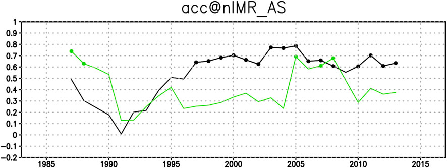
Figure 7. Decadal modulation of skill correlation (ACC) for the north India summer monsoon rainfall. The 9-year sliding skill correlation between the observed and SINTEX-F2-predicted north India (20°S–30°N, 75°W–90°E) summer monsoon rainfall anomaly in AS. The black (green) line shows the SINTEX-F2 January-start (April-start) prediction skill. Only significance > 90% is dotted.

The 1997-2016 period analyzed here corresponds to the availability of the OC-CCI v3.1 dataset used by Ogata et al. (2021). While this 20-year record is too short to evaluate slower climate modes such as the Interdecadal Pacific Oscillation or long-term regional trends evolving on multi-decadal (20–30 years) scales (Henley et al., 2015), it adequately captures the dominant interannual variability associated with ENSO, the IOD, and the ISMR (Ropelewski and Halpert, 1987; Saji et al., 1999; Krishnamurthy and Goswami, 2000; Pascual et al., 2000; Pascual et al., 2008). These modes, which are primary modulators of Bay-of-Bengal hydroclimate and cholera-conducive conditions, undergo several full cycles within 2 decades, providing a sufficient sampling basis for regression analysis. Future work will require longer, harmonized ocean-colour records to evaluate the stability of these relationships on multi-decadal timescales (Sathyendranath et al., 2019; Pauthenet et al., 2024).

Our results demonstrate that SWM forecast skill can be substantially enhanced by integrating a state-of-the-art seasonal climate prediction system. The ability to predict SWM conditions several months in advance has important implications for cholera risk management and for broader applications such as flood forecasting and agricultural planning.

Recent advances in seasonal prediction skill (Takaya et al., 2021), including multi-year predictability of ISMR driven by oceanic memory, further support the potential for extending the lead time and reliability of such forecasts. Moving forward, integrating dynamical climate predictions with ecosystem, crop, and disease models (Racault et al., 2017; Doi et al., 2020; Doi et al., 2022) offers a promising pathway to delivering robust early warning systems for climate-sensitive diseases such as cholera. On the other hand, the pathogen dynamics of V. cholerae cannot be explicitly resolved by the SWM index. This study primarily focused on the predictability of the SWM index as an environmental indicator favorable for V. cholerae, and although integrating epidemiological data is beyond the current scope, it is essential for developing an operational cholera early warning system. This study demonstrated the applicability of a climate prediction framework to assess environmental conditions associated with cholera risk, however epidemiological work will be essential for the development of operational cholera early warning systems.

Data availability statement

The original contributions presented in the study are included in the article/supplementary material, further inquiries can be directed to the corresponding author.

Author contributions

TO: Conceptualization, Formal Analysis, Investigation, Methodology, Writing – original draft, Writing – review and editing. M-FR: Conceptualization, Formal Analysis, Investigation, Methodology, Writing – original draft, Writing – review and editing. MN: Formal Analysis, Writing – original draft, Writing – review and editing. SB: Formal Analysis, Writing – original draft, Writing – review and editing.

Funding

The authors declare that financial support was received for the research and/or publication of this article. This study received financial support from multiple international agencies. It was funded under the Towards a Sustainable Earth (TaSE) initiative of the United Kingdom Research and Innovation (UKRI), the Department of Biotechnology (DBT) of India, and the Japan Science and Technology Agency (JST), specifically through the PODCAST project. Funding was provided by the Natural Environment Research Council (NERC) [Grant No. NE/S012567/1], JST [Grant No. JPMJBF18T4], and the ESA–Future Earth COP26 Demonstrator project (PODCAST-DEMO) [Grant No. ESA-2020-04]. This work also contributes to several broader collaborative initiatives, including the UKRI-NERC “Pathways of Dispersal for Cholera And Solution Tools (PODCAST)” project, the ESA–Future Earth PODCAST-DEMO effort, the GEO Blue Planet Water-associated Diseases Working Group (supported by the Partnership for Observation of the Global Ocean, POGO), Future Earth Coasts (a Global Research Project under Future Earth), and the Health Knowledge–Action Network within Future Earth.

Acknowledgements

The model datasets analyzed in this study are available upon reasonable request. Interested parties should contact the corresponding author (ogatatom@jamstec.go.jp) to obtain access. The authors express their gratitude to J. V. Ratnam for assistance in extracting the Indian monsoon rainfall data and to T. Doi for providing the SINTEX-F2 forecast outputs. SINTEX-F2 seasonal prediction integration was conducted on the Earth Simulator with the support of JAMSTEC.

Conflict of interest

The authors declare that the research was conducted in the absence of any commercial or financial relationships that could be construed as a potential conflict of interest.

The author(s) declared that they were an editorial board member of Frontiers, at the time of submission. This had no impact on the peer review process and the final decision.

Generative AI statement

The authors declare that Generative AI was used in the creation of this manuscript. To reduce and avoid self plagiarism, we used AI’s help for English editing. The report showed ∼9% similarity with Ogata et al., 2021, which should be sufficiently low to argue.

Any alternative text (alt text) provided alongside figures in this article has been generated by Frontiers with the support of artificial intelligence and reasonable efforts have been made to ensure accuracy, including review by the authors wherever possible. If you identify any issues, please contact us.

Publisher’s note

All claims expressed in this article are solely those of the authors and do not necessarily represent those of their affiliated organizations, or those of the publisher, the editors and the reviewers. Any product that may be evaluated in this article, or claim that may be made by its manufacturer, is not guaranteed or endorsed by the publisher.

References

Alexander, M. A., Vimont, D. J., Chang, P., and Scott, J. D. (2010). The impact of extratropical atmospheric variability on ENSO: testing the seasonal footprinting mechanism using coupled model experiments. J. Clim. 23 (11), 2885–2901. doi:10.1175/2010JCLI3205.1

CrossRef Full Text | Google Scholar

Ali, M., Nelson, A. R., Lopez, A. L., and Sack, D. A. (2015). Updated global burden of cholera in endemic countries. PLoS Neglected Tropical Diseases 9 (6), e0003832. doi:10.1371/journal.pntd.0003832

PubMed Abstract | CrossRef Full Text | Google Scholar

Ashok, K., Guan, Z., and Yamagata, T. (2001). Impact of the Indian Ocean dipole on the relationship between the Indian monsoon rainfall and ENSO. Geophys. Research Letters 28 (23), 4499–4502. doi:10.1029/2001GL013294

CrossRef Full Text | Google Scholar

Ashok, K., Behera, S. K., Rao, S. A., Weng, H., and Yamagata, T. (2007). El niño modoki and its possible teleconnection. J. Geophys. Res. Oceans 112 (C11). doi:10.1029/2006JC003798

CrossRef Full Text | Google Scholar

Cane, M. A., Zebiak, S. E., and Dolan, S. C. (1986). Experimental forecasts of EL nino. Nature 321 (6073), 827–832. doi:10.1038/321827a0

CrossRef Full Text | Google Scholar

Colwell, R. R. (1996). Global climate and infectious disease: the cholera paradigm. Science 274 (5295), 2025–2031. doi:10.1126/science.274.5295.2025

PubMed Abstract | CrossRef Full Text | Google Scholar

Darshana, P., Chowdary, J. S., Gnanaseelan, C., Parekh, A., and Srinivas, G. (2020). Interdecadal modulation of the Indo-western Pacific Ocean capacitor mode and its influence on Indian summer monsoon rainfall. Clim. Dyn. 54, 1761–1777. doi:10.1007/s00382-019-05085-5

CrossRef Full Text | Google Scholar

Doi, T., Storto, A., Behera, S. K., Navarra, A., and Yamagata, T. (2017). Improved prediction of the Indian Ocean dipole mode by use of subsurface ocean observations. J. Clim. 30 (19), 7953–7970. doi:10.1175/JCLI-D-16-0915.1

CrossRef Full Text | Google Scholar

Doi, T., Sakurai, G., and Iizumi, T. (2020). Seasonal predictability of four major crop yields worldwide by a hybrid system of dynamical climate prediction and eco-physiological crop-growth simulation. Front. Sustain. Food Syst. 4, 84. doi:10.3389/fsufs.2020.00084

CrossRef Full Text | Google Scholar

Doi, T., Behera, S. K., and Yamagata, T. (2022). On the predictability of the extreme drought in East Africa during the short rains season. Geophys. Res. Lett. 49 (22), e2022GL100905. doi:10.1029/2022GL100905

CrossRef Full Text | Google Scholar

Domman, D., Quilici, M. L., Dorman, M. J., Njamkepo, E., Mutreja, A., Mather, A. E., et al. (2017). Integrated view of Vibrio cholerae in the americas. Science 358 (6364), 789–793. doi:10.1126/science.aao2136

PubMed Abstract | CrossRef Full Text | Google Scholar

Fichefet, T., and Maqueda, M. M. (1997). Sensitivity of a global sea ice model to the treatment of ice thermodynamics and dynamics. J. Geophys. Res. Oceans 102 (C6), 12609–12646. doi:10.1029/97JC00480

CrossRef Full Text | Google Scholar

Good, S. A., Martin, M. J., and Rayner, N. A. (2013). EN4: quality controlled ocean temperature and salinity profiles and monthly objective analyses with uncertainty estimates. J. Geophys. Res. Oceans 118 (12), 6704–6716. doi:10.1002/2013JC009067

CrossRef Full Text | Google Scholar

Henley, B. J., Gergis, J., Karoly, D. J., Power, S., Kennedy, J., and Folland, C. K. (2015). A tripole index for the interdecadal Pacific oscillation. Clim. Dyn. 45 (11), 3077–3090. doi:10.1007/s00382-015-2525-1

CrossRef Full Text | Google Scholar

Jutla, A., Akanda, A. S., Huq, A., Faruque, A. S. G., Colwell, R., and Islam, S. (2013). A water marker monitored by satellites to predict seasonal endemic cholera. Remote Sens. Lett. 4 (8), 822–831. doi:10.1080/2150704X.2013.802097

PubMed Abstract | CrossRef Full Text | Google Scholar

Kao, H. Y., and Yu, J. Y. (2009). Contrasting eastern-Pacific and central-Pacific types of ENSO. J. Clim. 22 (3), 615–632. doi:10.1175/2008JCLI2309.1

CrossRef Full Text | Google Scholar

Kawamura, R. (1998). A possible mechanism of the Asian summer monsoon-ENSO coupling. J. Meteorological Soc. Jpn. Ser. II 76 (6), 1009–1027. doi:10.2151/jmsj1965.76.6_1009

CrossRef Full Text | Google Scholar

Krishnamurthy, V., and Goswami, B. N. (2000). Indian Monsoon–ENSO relationship on interdecadal timescale. J. Clim. 13 (3), 579–595. doi:10.1175/1520-0442(2000)013%253C0579:IMEROI%253E2.0.CO;2

CrossRef Full Text | Google Scholar

Kutner, M. H., Nachtsheim, C. J., Neter, J., and Li, W. (2005). Applied linear statistical models. Boston, MA: McGraw-Hill/Irwin.

Google Scholar

Luo, J.-J., Masson, S., Behera, S. K., and Yamagata, T. (2008). Extended ENSO predictions using a fully coupled ocean–atmosphere model. J. Clim. 21 (1), 84–93. doi:10.1175/2007JCLI1412.1

CrossRef Full Text | Google Scholar

Madec, G. (2008). NEMO reference manual, ocean dynamics component: NEMO-OPA. Preliminary version. Note du Pole de modélisation, 27. France: Institut Pierre-Simon Laplace IPSL.

Google Scholar

Mantua, N. J., and Hare, S. R. (2002). The Pacific decadal oscillation. J. Oceanography 58, 35–44. doi:10.1023/A:1015820616384

CrossRef Full Text | Google Scholar

Martinez, P. P., Reiner, R. C., Cash, B. A., Rodó, X., Shahjahan Mondal, M., Roy, M., et al. (2017). Cholera forecast for Dhaka, Bangladesh, with the 2015-2016 El niño: lessons learned. PLOS ONE 12 (3), e0172355. doi:10.1371/journal.pone.0172355

PubMed Abstract | CrossRef Full Text | Google Scholar

Masson, S., Terray, P., Madec, G., Luo, J. J., Yamagata, T., and Takahashi, K. (2012). Impact of intra-daily SST variability on ENSO characteristics in a coupled model. Clim. Dynamics 39, 681–707. doi:10.1007/s00382-011-1247-2

CrossRef Full Text | Google Scholar

Mutreja, A., Kim, D. W., Thomson, N. R., Connor, T. R., Lee, J. H., Kariuki, S., et al. (2011). Evidence for several waves of global transmission in the seventh cholera pandemic. Nature 477 (7365), 462–465. doi:10.1038/nature10392

PubMed Abstract | CrossRef Full Text | Google Scholar

Ogata, T., Doi, T., Morioka, Y., and Behera, S. (2019). Mid-latitude source of the ENSO-spread in SINTEX-F ensemble predictions. Clim. Dyn. 52, 2613–2630. doi:10.1007/s00382-018-4280-6

CrossRef Full Text | Google Scholar

Ogata, T., Racault, M. F., Nonaka, M., and Behera, S. (2021). Climate precursors of satellite water marker index for spring cholera outbreak in northern Bay of Bengal coastal regions. Int. J. Environ. Res. Public Health 18 (19), 10201. doi:10.3390/ijerph181910201

PubMed Abstract | CrossRef Full Text | Google Scholar

Pai, D. S., Rajeevan, M., Sreejith, O. P., Mukhopadhyay, B., and Satbha, N. S. (2014). Development of a new high spatial resolution (0.25× 0.25) long period (1901-2010) daily gridded rainfall data set over India and its comparison with existing data sets over the region. Mausam 65 (1), 1–18. doi:10.54302/mausam.v65i1.851

CrossRef Full Text | Google Scholar

Pascual, M., Rodó, X., Ellner, S. P., Colwell, R., and Bouma, M. J. (2000). Cholera dynamics and El niño-southern oscillation. Sci. (New York, N.Y.) 289 (5485), 1766–1769. doi:10.1126/science.289.5485.1766

PubMed Abstract | CrossRef Full Text | Google Scholar

Pascual, M., Bouma, M. J., and Dobson, A. P. (2002). Cholera and climate: revisiting the quantitative evidence. Microbes Infection 4 (2), 237–245. doi:10.1016/S1286-4579(01)01533-7

PubMed Abstract | CrossRef Full Text | Google Scholar

Pascual, M., Chaves, L. F., Cash, B., Rodó, X., and Yunus, M. (2008). Predicting endemic cholera: the role of climate variability and disease dynamics. Clim. Res. 36 (2), 131–140. doi:10.3354/cr00730

CrossRef Full Text | Google Scholar

Pauthenet, E., Martinez, E., Gorgues, T., Roussillon, J., Drumetz, L., Fablet, R., et al. (2024). Contrasted trends in Chlorophyll-a satellite products. Geophys. Res. Lett. 51 (14), e2024GL108916. doi:10.1029/2024GL108916

CrossRef Full Text | Google Scholar

Racault, M. F., Sathyendranath, S., Brewin, R. J., Raitsos, D. E., Jackson, T., and Platt, T. (2017). Impact of El niño variability on Oceanic phytoplankton. Front. Mar. Sci. 4, 133. doi:10.3389/fmars.2017.00133

CrossRef Full Text | Google Scholar

Racault, M.-F., Abdulaziz, A., George, G., Menon, N., C, J., Punathil, M., et al. (2019). Environmental reservoirs of vibrio cholerae: challenges and opportunities for ocean-color remote sensing. Remote Sens. 11 (23), 2763. doi:10.3390/rs11232763

CrossRef Full Text | Google Scholar

Reynolds, R. W., Rayner, N. A., Smith, T. M., Stokes, D. C., and Wang, W. (2002). An improved in situ and satellite SST analysis for climate. J. Climate 15 (13), 1609–1625. doi:10.1175/1520-0442(2002)015<1609:aiisas>2.0.co;2

CrossRef Full Text | Google Scholar

Roeckner, E., Bäuml, G., Bonaventura, L., Brokopf, R., Esch, M., and Giorgetta, M. (2003). The atmospheric general circulation model ECHAM 5. PART I: model description.

Google Scholar

Ropelewski, C. F., and Halpert, M. S. (1987). Global and regional scale precipitation patterns associated with the El niño/southern oscillation. Available online at: https://journals.ametsoc.org/view/journals/mwre/115/8/1520-0493_1987_115_1606_garspp_2_0_co_2.xml.

Google Scholar

Saji, N. H., Goswami, B. N., Vinayachandran, P. N., and Yamagata, T. (1999). A dipole mode in the tropical Indian Ocean. Nature 401 (6751), 360–363. doi:10.1038/43854

PubMed Abstract | CrossRef Full Text | Google Scholar

Sasaki, W., Richards, K. J., and Luo, J. J. (2013). Impact of vertical mixing induced by small vertical scale structures above and within the equatorial thermocline on the tropical Pacific in a CGCM. Clim. Dynamics 41, 443–453. doi:10.1007/s00382-012-1593-8

CrossRef Full Text | Google Scholar

Sathyendranath, S., Brewin, R. J., Brockmann, C., Brotas, V., Calton, B., Chuprin, A., et al. (2019). An ocean-colour time series for use in climate studies: the experience of the ocean-colour climate change initiative (OC-CCI). Sensors 19 (19), 4285. doi:10.3390/s19194285

PubMed Abstract | CrossRef Full Text | Google Scholar

Shackleton, D., Economou, T., Memon, F. A., Chen, A., Dutta, S., Kanungo, S., et al. (2023). Seasonality of cholera in kolkata and the influence of climate. BMC Infect. Dis. 23 (1), 572. doi:10.1186/s12879-023-08532-1

PubMed Abstract | CrossRef Full Text | Google Scholar

Shen, X., Kimoto, M., and Sumi, A. (1998). Role of land surface processes associated with interannual variability of broad-scale Asian summer monsoon as simulated by the CCSR/NIES AGCM. J. Meteorological Soc. Jpn. Ser. II 76 (2), 217–236. doi:10.2151/jmsj1965.76.2_217

CrossRef Full Text | Google Scholar

Takaya, Y., Kosaka, Y., Watanabe, M., and Maeda, S. (2021). Skilful predictions of the Asian summer monsoon one year ahead. Nat. Commun. 12 (1), 2094. doi:10.1038/s41467-021-22299-6

PubMed Abstract | CrossRef Full Text | Google Scholar

Vezzulli, L., Grande, C., Reid, P. C., Hélaouët, P., Edwards, M., Höfle, M. G., et al. (2016). Climate influence on vibrio and associated human diseases during the past half-century in the coastal north Atlantic. Proc. Natl. Acad. Sci. 113 (34), E5062–E5071. doi:10.1073/pnas.1609157113

PubMed Abstract | CrossRef Full Text | Google Scholar