 Hannes P. T. De Deurwaerder1,2*
 Marco D. Visser1,3
 Félicien Meunier2
 Matteo Detto1
 Pedro Hervé-Fernández4,5,6
 Pascal Boeckx4
 Hans Verbeeck2
- 1Department of Ecology and Evolutionary Biology, Princeton University, Princeton, NJ, United States
- 2CAVElab–Computational and Applied Vegetation Ecology, Faculty of Bioscience Engineering, Ghent University, Ghent, Belgium
- 3Institute of Environmental Sciences, Leiden University, Leiden, Netherlands
- 4ISOFYS–Isotope Bioscience Laboratory, Faculty of Bioscience Engineering, Ghent University, Ghent, Belgium
- 5School of Environment and Sustainability, Global Institute for Water Security, University of Saskatchewan, Saskatoon, SK, Canada
- 6Facultad de Artes Liberales, Universidad Adolfo Ibáñez, Santiago, Chile
The vertical distribution of absorbing roots is one of the most influential plant traits determining plant strategy to access below ground resources. Yet little is known of natural variability in root distribution since collecting field data is challenging and labor-intensive. Studying stable water isotope compositions in plants could offer a cost-effective and practical solution to estimate the absorbing root surfaces distribution. However, such an approach requires developing realistic inverse modeling techniques that enable robust estimation of rooting distributions and associated uncertainty from xylem water isotopic composition observations. This study introduces an inverse modeling method that supports the assessment of the root allocation parameter (β) that defines the exponential vertical decay of a plants’ absorbing root surfaces distribution with soil depth. The method requires measurements obtained from xylem and soil water isotope composition, soil water potentials, and sap flow velocities when plants’ xylem water is sampled at a certain height above the rooting point. In a simulation study, we show that the approach can provide unbiased estimates of β and its associated uncertainty due to measuring errors and unmeasured environmental factors that can impact the xylem water isotopic data. We also recommend improving the accuracy and power of β estimation, highlighting the need for considering accurate soil water potential and sap flow monitoring. Finally, we apply the inverse modeling method to xylem water isotope data of lianas and trees collected in French Guiana. Our work shows that the inverse modeling procedure provides a robust analytical and statistical framework to estimate β. The method accounts for potential bias due to extraction errors and unmeasured environmental factors, which improves the viability of using stable water isotope compositions to estimate the distribution of absorbing root surfaces complementary to the assessment of relative root water uptake profiles.
Introduction
The absorbing root surfaces distribution (AR), i.e., those surfaces of a plants’ root system that support water uptake, is a pivotal plant characteristic that determines the plant species’ nutrient and water acquisition strategy. Investments in competitive advantage usually imply maximizing the upper soil layer’s exploitation, where the concentration of nutrients is generally highest (Jobbagy and Jackson, 2001). However, this comes at the cost of drought tolerance since upper layers are generally more drought-prone than deeper soil layers with more stable water reserves (Fogel, 1985). Accurate measures of A_R are thus needed to characterize specific plant competitive strength and drought response.
Unfortunately, data on root distributions in general—and on A_R in specific—is scarce, and little is known about the intra- and interspecific variability in A_R across different environments (Böhm, 2012). This paucity is caused in part by the available techniques to study root distributions of individual plants, which are often destructive, expensive, and labor intensive (Cabal et al., 2021). Root excavation, for example, holds the highest promise of most accurately characterizing a plant’s natural root distribution (Böhm, 2012). However, the associated workload limits its practical application to small sample sizes and small habitus plants, e.g., annual plants, crops, and young trees. As an illustration, Preston (1942) estimated that one laborer requires approximately 5 weeks to fully excavate and examine the root system of single 15-year-old lodgepole pine. These time and labor disadvantages have led to the development of many other direct and indirect in situ techniques, such as rhizotron systems, acoustic and electromagnetic tomography, the auger method, or the use of non-radioactive tracers (reviewed in Cabal et al., 2021). However, while these techniques provide a less invasive alternative to root excavation, they generally fall short in the level of details they can provide on the distribution of the individual absorbing root surfaces.
A relatively straightforward technique to relate relative root water uptake (RWU, which is inextricably linked toAR) with soil depth is using stable water isotope composition as non-radioactive tracers. Ehleringer and Dawson (1992) described the simplicity of the technique, which lies in a direct relationship between the isotopic composition of the xylem sap (δxyl) and the isotopic composition observed in soil water (δsoil) along with a soil depth profile. Common approaches assume that xylem water is a proportional mixture of δsoil from the various depths at which roots absorb water (Phillips and Gregg, 2003). The approach requires: (i) the occurrence of a natural isotopic gradient in the soil generated by topsoil water evaporation (Beyer et al., 2018); and (ii) the absence of processes that alter the xylem water isotope composition while entering the plant or during transport along the plant hydraulic system (Wershaw et al., 1966; Zimmermann et al., 1967; White et al., 1985; Dawson and Ehleringer, 1991; Walker and Richardson, 1991; Dawson et al., 2002; Zhao et al., 2016). Requirements (i) and (ii) generally limit the technique to lignified plants and implementation during rain-free periods after sufficient soil evaporation has occurred. However, these conditions still allow strong flexibility and usability across multiple temporal and spatial scales (Dawson et al., 2002). Its moderate labor and time investment allows sampling of more and larger plant species far beyond what is possible with root excavation.
However, the robustness of stable water isotope techniques has been recently questioned (Penna et al., 2018; von Freyberg et al., 2020). An increasing number of studies discuss a potential mismatch between available water sources and isotopically depleted compositions in xylem water. Hypothetical discrepancies have resulted from: isotopic discrimination at root-level (Allison et al., 1983; Vargas et al., 2017) or by associated mycorrhizae (Poca et al., 2019), and by internal mixing of xylem water with isotopically depleted water reserves stored in stem tissue (Barbeta et al., 2020; Knighton et al., 2020). The link between source water and the isotopic composition of xylem water (δxyl) can be further obscured by pronounced water-transport lags (Meinzer et al., 2006; Gaines et al., 2016; Magh et al., 2020; Marshall et al., 2020; Mennekes et al., 2021) or possible excessive intra-individual variance in δxyl due to variable RWU dynamics caused by fluctuating biophysical factors, frequently overlooked in isotopic studies (e.g., soil water potentials, vapor pressure deficits and sap flow dynamics) (De Deurwaerder et al., 2020). This growing body of literature suggests that standard sampling methods may deliver biased estimates of RWU profiles while simultaneously underestimating uncertainty among species, biomes, or seasonality. Therefore, a real need exists to develop methods that accurately estimate A_R and associated uncertainty in the face of unmeasured biophysical factors that affect δxyl.
Coupling stable isotope measurements to biophysical models (e.g., RAPID algorithm) could support the inverse reconstruction of absorbing root surfaces distribution, A_R, and the assessment of their active contribution to RWU (Ogle et al., 2004). Such a coupled technique has enormous potential to build a fundamental understanding of spatial and temporal variability in water competition strategy amongst and within plant species. To the best of our knowledge, only one previous study endeavored to develop such a tool (Ogle et al., 2004). However, it did not account for unmeasured biophysical factors that affect δxyl potentially leading to biased estimates. Here we adopt a mechanistic model for uptake and transport of stable water composition through plants (De Deurwaerder et al., 2020) and use simulations to show that this inverse modeling method offers estimates of β, the allocation parameter which defines the exponential vertical decay of a plants’ A_R while (1) accounting for the xylem water isotopic variance within plants, as well as (2) uncertainties in isotopic measurements and (3) biophysical parameters, e.g., sap flow dynamics. We further provide guidelines to improve sampling design in future studies. Finally, we show how the model can validate previous results by re-analyzing a case study in French Guiana for tree and liana growth forms. This study suggests that previous methods underestimated the uncertainty in mean xylem water δ2H and δ18O provided by De Deurwaerder et al. (2018). The applied inverse method is provided as an open-source code (see GitHub repository HannesDeDeurwaerder/iSWIFT).
Materials and Methods
The SWIFT model links xylem water isotope compositions (δxyl) to an allocation parameter β, that defines the exponential vertical decay of A_R with soil depth. We give a brief overview of the model in box 1, restricted to key equations expressed for the hydrogen isotope composition in xylem and soil water (δ2HX and δ2HS). Subsequently, we describe the numerical inversion needed to generate estimates of β from δxyl and δsoil. Here, we evaluate how increased levels of variable range restrictions improve estimates of β, followed by a power analysis to inform to which extent β should differ between groups of plants subject to similar edaphic conditions to observe statistical differences in δxyl. Both analyses can help guide future study design optimization. Finally, we introduce a practical case study in French Guiana. We maintain the following notation in the subscripts of presented variables: the medium through which water travels is indicated by uppercase fonts, while lowercase fonts highlight the units of time and distance: X for xylem, R for root, S for soil, h for stem height, t for time, and i for the corresponding soil layer. A complete overview of variables, definitions and units is given in Supplementary Table 1, and details on the SWIFT model can be found in Supplementary Appendix A and De Deurwaerder et al. (2020).
BOX 1. SWIFT in a nutshell.
SWIFT (Stable Water Isotope Fluctuation within Trees) generates paired predictions of xylem water isotope composition (δxyl) and the respective sampling error (ξ):
In SWIFT δxyl is a function of the relative absorptive root surfaces distribution with soil depth (AR), determined by allocation parameter β, and a set of biophysical variables (χ) that influence δxyl other than β (see Table 1). We distinguish three distinct groups of biophysical variables in χ:
• Physical: soil properties, spatial variability in the gradients of soil water isotope composition (δSoil), and in the soil water potential (ΨS) with soil depth, hereafter indicated as soil heterogeneity.
• Biological: plant trait, i.e., the sapwood area (ASAPWOOD), the lumen fraction (LF), the effective root radial conductivity (kR) and the sap flow dynamics (SF).
• Sampling: sampling strategy related variables, i.e., the height (hos) and time (t) of the day during sampling.
The biophysical variables are the same for both water isotopes (χδ18Oand χδ2H) except for the isotopic soil profiles (δSoil;δ2HS&δ18OS). The error term ξ includes cryogenic water extraction errors, since these errors unavoidably occur during the extraction procedure (Orlowski et al., 2013). The magnitude of these errors are within the conservative range of 3 and 0.3‰ for δ2H and δ18O, respectively (Araguás-Araguás et al., 1995). In the Monte Carlo method these errors are simulated as independent Gaussian random variables to generate δxyl values.
Relation between AR and β. The discrete representation of A_R is a function of the total absorbing root area available to the focal plant (ARtot) allocated via parameter β over all soil depths, zi (cm), discretized in layers of thickness △z as follows (Jackson et al., 1996):
Key mechanics. SWIFT couples (i) a standard multi-source mixing model approach (Phillips and Gregg, 2003) which composes the weighted isotope composition entering the stem base of a plant of the relative quantities of water taken up and the respective δsoil at each soil layer (i = 1,2,..,n), with (ii) a mechanistic plant hydraulic module to simulate the impact of root water uptake (RWU) and xylem transport dynamics on δxyl.
The deuterium isotope composition of water entering the stem base of a plant (δ2HX,0,t) at time t is a weighted sum of the product of the relative water taken up (Fi,t) from each layer and the corresponding δ2HS,i. Assuming soil conductivity is much bigger than kR, a simplified model for the δ2HX,0,t can be given as (for a complete formulation that includes soil and root conductivity, see Supplementary Appendix A):
Fi,t depends on (i) the relative amount of absorbing root surface per soil layer available to the plant (βzi), and (ii) the ability of these root surfaces to uptake water based on the water potential gradient between root xylem and soil (△Ψi,t). In the present model, root water potentials show diurnal variability driven by plant responses to fluctuating abiotic conditions (i.e., vapor pressure deficit). The latter leads to a variable δ2HX,0,t which then propagates along the stem of the plant, causing a lag between the isotope compositions entering the plant and that of extracted δxyl samples taken at different heights. SWIFT takes this into account by computing the time, τ, a molecule of 2H takes to travel from where it was extracted, δ2HX,0,t, to the height h where samples were taken, δ2HX,h,t, using modeled or observed sap flow velocities.
Merits of using SWIFT. The SWIFT implementation considers that variance in the χ variables can indeed (i) transmit in differences in a plant’s root water uptake ability and rates at different soil layers (i.e., ΨS, δ2HS,i, kR and SF) which causes variance independent of β, and (ii) account for transportation lag and optimized sampling (i.e., ASAPWOOD, LF, SF, hos, and t). Both (i) and (ii) are generally disregarded in stable water isotope studies, leading to potential biases in derived insights from δxyl samples, hence in RWU and β.
Inverse SWIFT: Numerical Model Inversion and Likelihood Estimation
The goal is to estimate the relative shape of absorbing root surfaces distribution by numerical inversion of the allocation parameter β, given a set of measured δxyl collected from plants in the field (Figure 1). We start with a vector C consisting of paired δ2Hx and δ18Ox observations, and assume C to be a bi-variate random variable with a conditional probability density function P(C|βtrue,χtrue) determined by the “true” allocation parameter, βtrue, and natural occurring variance in the local set of biophysical variables, χtrue (Figure 1A).
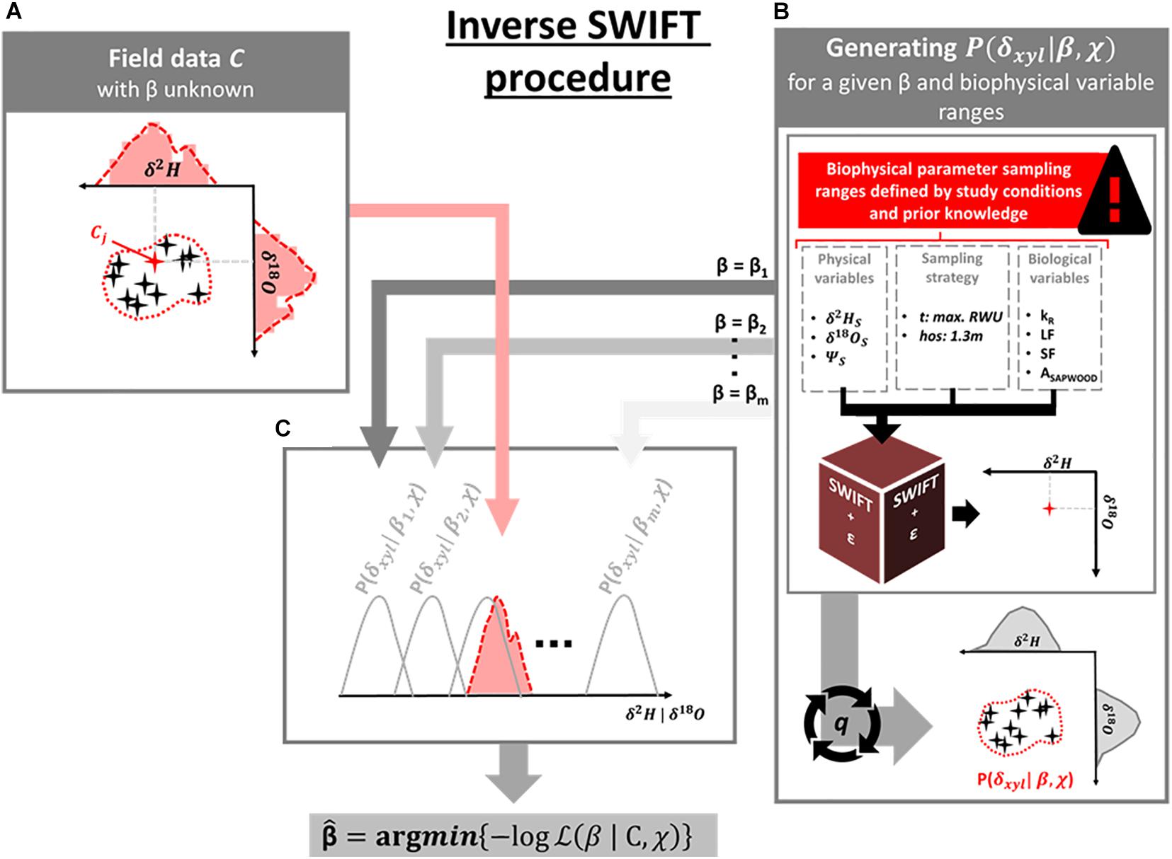
Figure 1. Schematic overview of the Inverse SWIFT procedure which supports estimation of the plant groups’ mean allocation parameter β (which defines the exponential vertical decay of the distribution of absorbing root surface with soil depth) from the respective xylem water isotopic compositions [(δxyl; being δ2H and/or δ18O, subplot (A)]. Specifically, a model that couples a standard multi-source mixing model with a mechanistic plant hydraulic model, e.g., the SWIFT model, allows for the generation of theoretical xylem water isotopic field data for a given β and a set of biophysical model variables (χ) (B). In this way, conditional density probability distributions (P(δxyl|β,χ)) are established for a range of β-values to which field data C can be matched (C). Theβ-value which correspond to the (P(δxyl|β,χ)) which minimizes the log-likelihood function provides the best β-estimate () of the studied plant group.
Subsequently, we consider Equations 1–3 (Box 1) to generate distributions of synthetic δxyl values that correspond to a wide range of biophysical parameters (χ) which prior distributions are user-specified or measured (Supplementary Table 2) and given a specific value of β (Figure 1B). These distributions are defined as conditional probability density distributions where P(δxyl|β,χ) represents the range of possible δxyl values generated by the SWIFT model (hereafter “Synthetic δxyl”), given a specific β and uncertainty in χ. We then vary the parameter β, generating new distributions associated with each considered β-value, P(δxyl|β,χ), until we find the distribution that maximizes the likelihood of observing the field samples C (Figure 1C). This maximum likelihood estimate of β (hereafter indicated as ) is then assumed to be the best approximation of βtrue. The distribution of each biophysical variable in χ can be based on prior measurements of the studied system or set as uninformative uniform distributions when no prior knowledge is available. A schematic workflow of this Inverse SWIFT approach is provided in Figure 1.
Likelihood and Model Optimization
The inversion procedure starts by numerically generating a vector of paired values (see Equation S1) for a given value of β, with other parameters drawn by q Monte-Carlo simulations from the user assigned or measured distributions of each biophysical variable χ. Here, we set q to 250, and the distributions of χ are given in Supplementary Table 2. The conditional density probability distributions P(δxyl|β,χ) are computed using a bi-variate kernel density estimator (i.e., the kde function of the “ks” R-package, Duong, 2007). The likelihood of observing C, the paired δxyl values from field data of k samples (j = 1, 2, …, k), is then defined as:
The β of the P(δxyl|β,χ) which minimizes the sum of the negative log-likelihood function, given the observed C, is then considered as the best estimate of βtrue, i.e., .
The search of β values is restricted to the range 0.905–0.995, according to the global analysis in Jackson et al. (1996). A one-dimensional general-purpose optimization method was used to find minima for Equation 2 (“brent” method in the “stats” package optim function, R Core Team, 2017).
Bias Evaluation in the Inversion Procedure
To quantify how the three distinct parameter sets defined earlier–physical, biological, and sampling (Box 1)–influence the likelihood, bias, and power, we generated sets of synthetic δxyl data (CSYN) with known values of β (βtrue and χtrue; βtrue set at 0.966. The selected value is representative for temperate deciduous forest rooting profiles after Jackson et al. (1996; see Table 1 and Supplementary Table 2) and then inversely estimated and associated likelihood profiles. During this procedure, the following four scenarios of increasing variable restriction of χ are considered and represent different levels of prior knowledge on the parameter set χ.
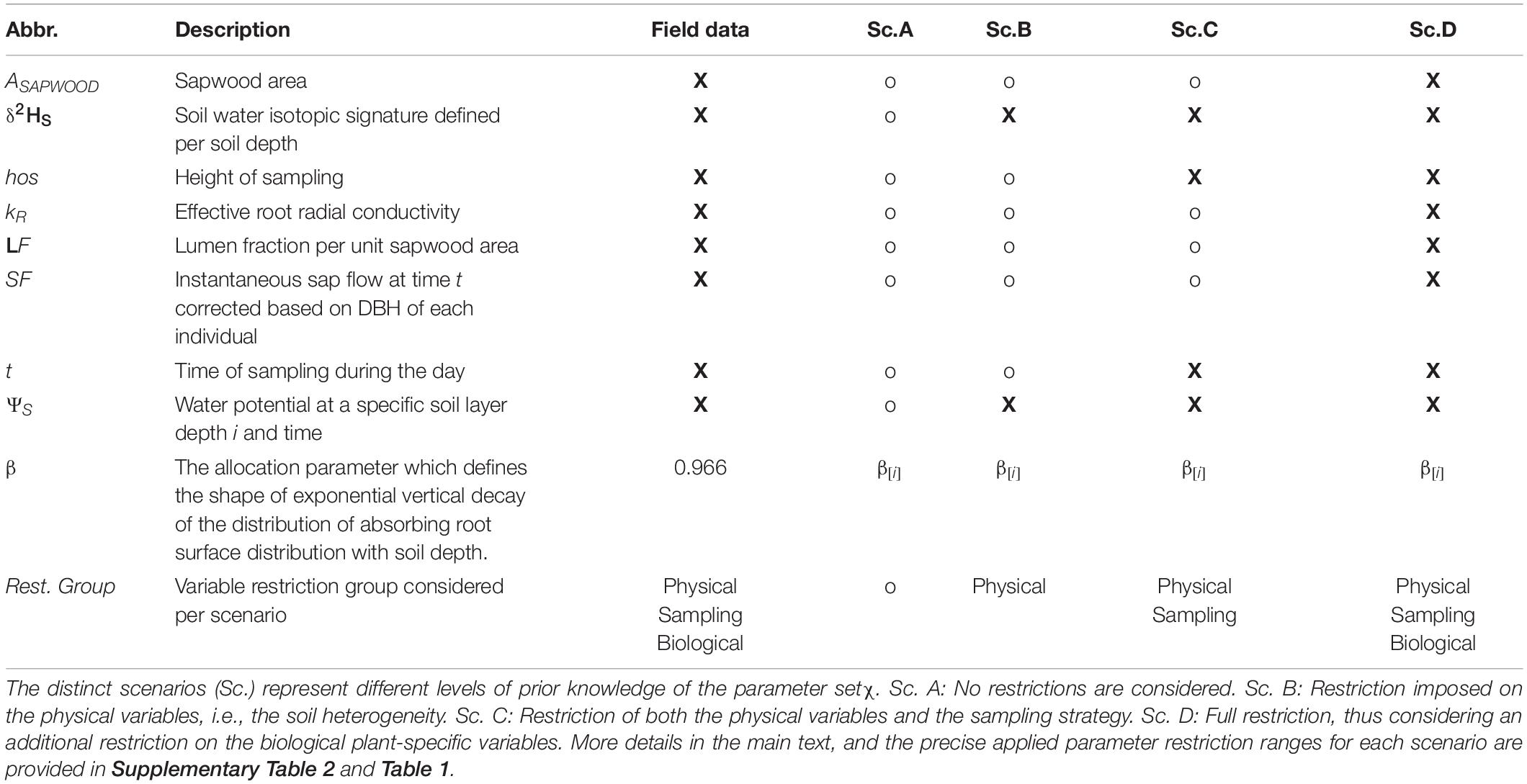
Table 1. Overview of the variable restrictions (X: restricted; o: non-restricted) considered within the inverse SWIFT procedure to simulate synthetic field data and corresponding conditional density probability distributions P(δxyl|β,χ).
Scenario A: No variable range restrictions. This scenario assumes no prior knowledge of the system, except for δSoil and soil water potential (ΨS) profiles with soil depth. This corresponds to the most common study conditions (Rothfuss and Javaux, 2017). Ideally, well-characterized δSoil-profiles from homogeneous soils yield the best results but in natural settings, soil heterogeneity can lead to high spatial variability which causes large random sampling errors. Therefore, we start from clearly defined empirical δ18OS and ΨS profiles, hereafter the “true profiles” (illustrated by those obtained by Meißner et al. (2012)) and sample more uncertain “observed” soils profiles (using ± 3 standard deviation from the true δ18OS and ΨS, profiles see functions Supplementary Table 2)—hereafter “heterogeneous profiles.” As we assume equilibrium conditions δ2HS profiles are deduced from δ18OS using the local meteoric water line (LMWL) (for details see Supplementary Appendix B).
Scenario B: Variable range restriction of the soil heterogeneity. Here the ΨS and δSoil-profiles are assumed to be characterized with higher precision. The input parameterization now considers narrow variance ranges, i.e., mean ± 1 standard deviation of the ΨS and δ18OS true profiles. Yet again, δ2HS profiles are calculated from δ18OS using the LMWL.
Scenario C: Variable range restriction by sampling strategy. Restricting sampling of δxyl–values to periods that correspond to maximum RWU activity may decrease bias (see De Deurwaerder et al., 2020). In this scenario, we assumed that the sampling strategy was optimized in timing (t) and the height of sampling (hos) targeting representative δxyl values representative for peak RWU. Specifically, the height of sampling is set at 1.3 m, which corresponds to the general practice of sampling trees at breast height. Subsequently, we define the sampling time by the moment the δxyl–values that correspond to the plant’s peak water uptake of the plant passes the 1.3 m sampling height, which depends on the plant’s sap flow velocity.
Scenario D: Variable range restriction of biophysical plant traits. Knowledge of natural variance in plant-specific input variables can be used to restrict the model. In practice this can be done via direct in situ measurement or through literature information. In this scenario, we consider the sapwood area (ASAPWOOD), the lumen fraction (LF), the effective root radial conductivity (kR) and the instantaneous sap flow (SF) known to a much better degree allowing restriction of their range and distribution (provided in Table 1 and Supplementary Table 2).
Bias in the was calculated as . We calculated the bias for different sample sizes (CSYN with 5, 25 and 50 samples) and all scenarios. Per scenario and sample size, we randomly assign aβtrue, inversely estimate and calculate bias for 500 independent simulations per scenario (with q = 250). The latter reveals which combination of sample size and set of variable restrictions (physical, biological, or sampling) yields the largest considerable estimation accuracy improvement.
Power Analysis
A power analysis quantifies the ability to distinguish between plant groups with different relative AR–profiles (as determined by β). Here we generate two sets of synthetic δxyl values which correspond to distinct plant groups which have similar χ, but differ in β. By inverse modeling, we computed the corresponding and via the inverse model approach as it would be done in actual study conditions. The power analysis consists of two parts. First, we quantified the minimal detectable difference (d), being the smallest statistical detectable difference between groups for each scenario. Here, d is the difference in and where the mean of one conditional density probability distributions P(δxyl|β,χ) is outside the 95% quantile of the other. Hence, we generated P() and P() for each scenario as described above (see section “Likelihood and Model Optimization”). Secondly, we calculated how often a significant difference would be detected for a different combination of β values under each scenario. We maintained the standard power level of 0.80 as a validation level for different sample sizes (i.e., 5, 25, and 50).
Case Study: Estimation of the Generic Rooting Depths for Trees and Lianas in French Guiana
In the case study, we examine two growth forms, lianas and trees, that strongly differ in traits that could bias RWU depth estimation, i.e., hydraulic properties and sap flow dynamics (Chen et al., 2015). We also evaluate differences in sampling strategy where a standard approach is compared to a setup where ΨS profiles were measured in Laussat, French Guiana, in 2017 (Supplementary Figures 3, 4). The two setups allow us to quantify the impact of different degrees of parameter restriction in the inverse model procedure.
Sampling Strategy Field Data
Setup A applies a standard setup that ignores soil properties, e.g., ΨS profile, and plant physiological processes that increase variance in δxyl. The latter is similar to the sampling strategy applied in De Deurwaerder et al. (2018). This standard method ignores uncertainty in the biophysical variables and uncertainty introduced by sampling. For instance, stem cores were taken at breast height for trees, while for lianas, sampling was done at various heights, which depended on branch accessibility for the climber. Sampling at different heights requires correction for the expected lag in transport (see Box 1), and not correcting for sampling height can lead to underestimation of uncertainty (De Deurwaerder et al., 2020). Here, insights in sap flow velocities and related biophysical variables (i.e., lumen area and root radial conductivity) would govern insights in daily variance in plant water potentials. The latter drives RWU dynamics, hence the incoming mixture of isotope compositions of tapped soil water sources. Such sap flow measurements would also support the characterization of the transportation lag essential for correctly matching δxyl with the driving abiotic conditions at the time of uptake. Hence, we expect that ignoring unmeasured biophysical variables and the sampling design can lead to an underestimation of the error in mean δxyl compared to using the inverse SWIFT method.
Setup B differs from A in that representative ΨS profiles were obtained from soil water potential sensors installed at the Paracou field station (French Guiana, period 15/09-15/10 2017, 3 setups of MPS-6 dielectric water potential sensors, Decagon Devices, Inc. Washington, United States). Given its similarities in edaphic and environmental conditions, the in situ ΨS monitored in Paracou is considered representative for the Laussat study site. Pooling all the data per monitoring depth (i.e., 15, 30, 45, 60, and 90 cm) provided ΨS averages and variance, allowing the construction of a representative ΨS profile for inverse SWIFT.
For both setups A and B, we estimated the uncertainty in mean δxyl values, tested whether significant differences were observed between lianas and trees which informs RWU depth and evaluated the influence of improved monitoring to restrict the unknown parameter space of our inverse model. In line with De Deurwaerder et al. (2018), we assume more inter- than intra growth form differences in rooting distributions. All samples were therefore clustered according to their growth form, and model parameterization was guided by growth form specific empirical data from literature. Further details on the study site, sampling strategy and extraction protocols are provided in Supplementary Appendix C.
Applying the Inverse Model
In both case study setups, we consider a moderately constrained version where various biophysical SWIFT input variables are obtained by reasoned assumptions from literature and measurements collected under similar conditions (Supplementary Table 3). In Supplementary Appendices B–D, we supply descriptions of the dual-isotope plots (Supplementary Figures 3, 4), applied data collection and processing which account for the observed δ2H offset (after Barbeta et al., 2019), as well as detailed information concerning datasets used for inverse SWIFT parameterization of both setups (Supplementary Table 3). This case study is restricted to clay plots as no representative ΨS data is available for sand plots needed to enable qualitative assessment of β. The lack of a ΨS profile obscures the link between absorbing root surfaces distribution and the water uptake activity and rates per soil layer, hence imposing a bias in which we are unable to quantify. Finally, the inverse SWIFT approach was performed for 10 independent iterations to quantify bias, where the average of all iterations represents the generic of the studied liana and tree communities.
Results
Model Simulation With Synthetic Field Data
The minima of log-likelihood profiles for each simulation showed a close to βtrue. Robust and unbiased will require some restrictions in the variable ranges and measurement uncertainty. In most cases, simulations show that log-likelihood curves tend to be flatter when little restrictions were applied (Figures 2, 3 and Supplementary Figure 2), implying significant uncertainty. The log-likelihood curves were generally steeper when soil heterogeneity (Sc. B) and an optimized sampling strategy (Sc. C) were considered. Interestingly, an increase in sample size had only a moderate effect on decreasing uncertainty (Figure 3) compared to applying other restrictions (Figures 2, 3 and Supplementary Figure 2), indicating that effort in reducing uncertainty in biophysical variables should be a priority. Bias was greatest with no variable range restrictions (scenario A), resulting in underestimation compared to βtrue (Figure 3), since the generated P(δxyl|β,χ) were skewed to more negative signatures (Figure 4B). The peak of P(δxyl|β,χ) narrows with increased scenario restrictions resulting in an improved ability to distinguish different datasets (Figure 4). Restriction of the soil heterogeneity reduced the width of P(δxyl|β,χ), albeit a distinct tail toward more depleted isotope compositions remained (Figure 4B). An optimized sampling strategy overcame this skewness (Figure 4C) and hence provided an improved which was no longer biased toward overestimation. As expected, the greatest restriction of the biophysical plant variables (Sc. D) yielded the lowest bias, although improvements from scenario C were modest (Figures 2–4).
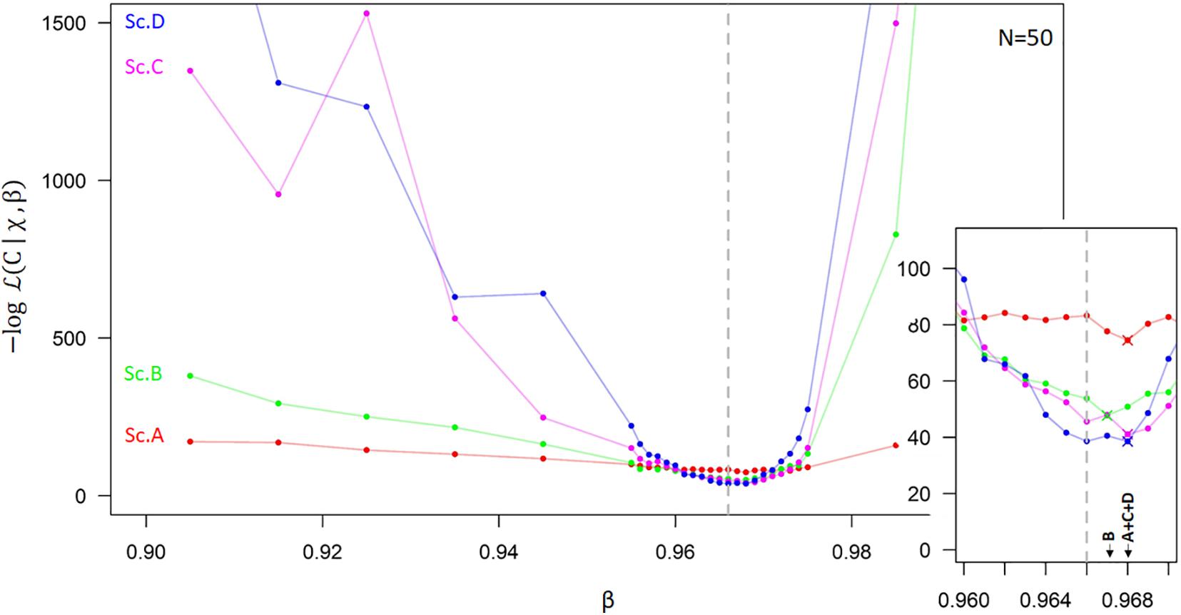
Figure 2. Example of a Log-likelihood curve (–log 𝓛(β|C,χ)) as a function of the allocation parameter β which defines the exponential vertical decay of the distribution of absorbing root surface with soil depth, under four different scenarios (Sc. A–D). The best β estimate (, has the minimal log-likelihood values shown for each scenario in a magnified panel (the true β is indicated by the dashed line, βtrue = 0.966). This figure represents a sample size (N) of 50 individuals. Supplementary Figures 2A,B shows similar likelihood profiles for smaller sample sizes. Sc. A: No restrictions are considered. Sc. B: Restriction imposed on the physical variables, i.e., the soil heterogeneity. Sc. C: Restriction of both the physical variables and the sampling strategy. Sc. D: Full restriction, thus considering an additional restriction on the biological plant-specific variables. More details in the main text and the applied parameter restriction for each scenario are given in Supplementary Table 2 and Table 1.
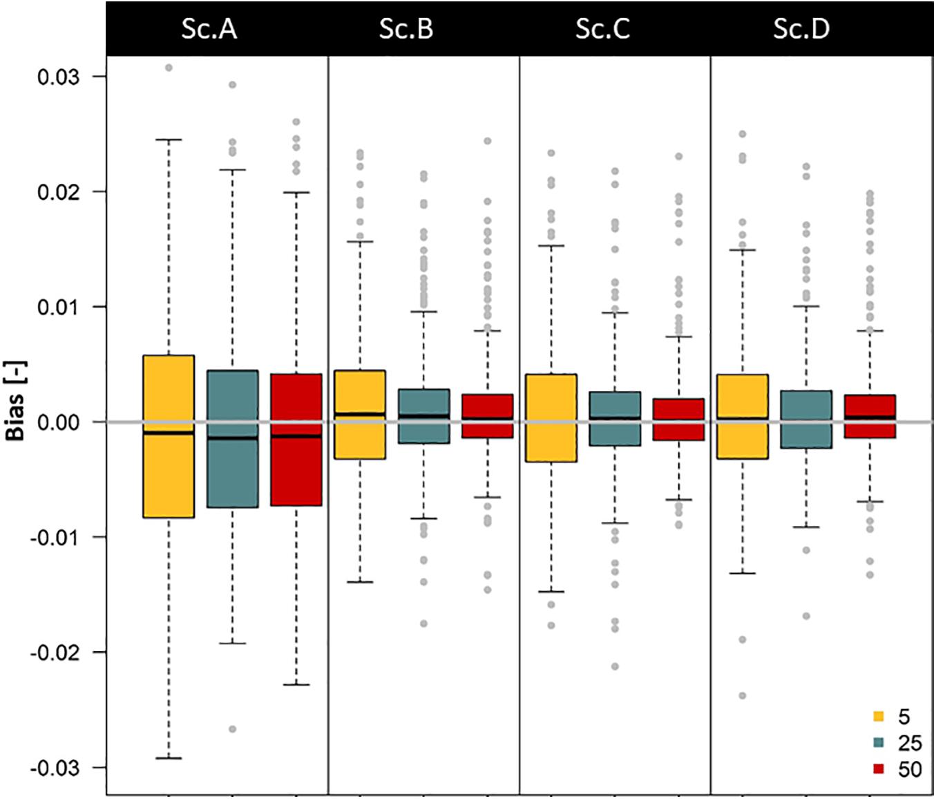
Figure 3. Boxplots showing the expected bias in β estimation () for four theoretical scenarios, bias decreases when key biophysical parameters (χ) are known or when the sample size increases. Sc. A: No variable range restrictions are considered. Sc. B: Restriction imposed on the physical variables, i.e., the soil heterogeneity. Sc. C: Restriction of both the physical variables and the sampling strategy. Sc. D: Full restriction, thus considering an additional restriction on the biological plant-specific variables. Different boxplots’ colors show the considered sample size (5: yellow, 25: blue, 50: red). Boxplots show Q25 - 1.5 IQR, Q25, Q50, Q75 and Q75 + 1.5 IQR values, with IQR the interquartile range. Outliers are provided as gray dots.
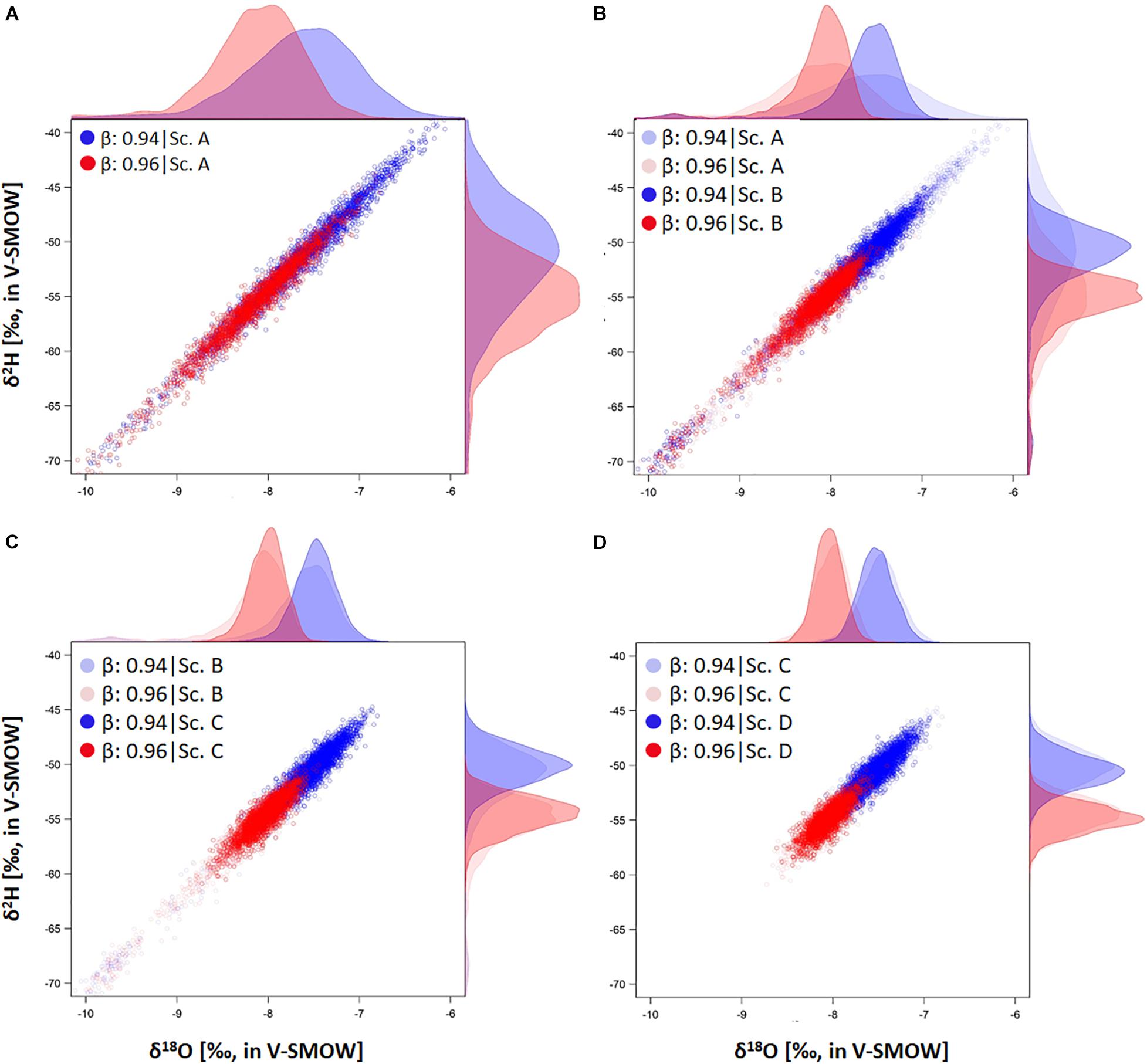
Figure 4. Representation of the simulated conditional probability distribution [i.e., P(δxyl|β,χ)] of xylem water isotope composition (δxyl) with two distinct profiles in absorbing root surface distribution, i.e., β = 0.94 ( ) and β = 0.96 (
 ). Each point represents an individual δxyl sample generated by the SWIFT model. Different panels (A–D) show the results for P(δxyl|β,χ) under different theoretical scenarios - Sc. A: No variable range restrictions are considered. Sc. B: Restriction imposed on the physical variables, i.e., the soil heterogeneity. Sc. C: Restriction of both the physical variables and the sampling strategy. Sc. D: Full restriction, thus considering an additional restriction on the biological plant-specific variables. Shaded colored probability distributions in panel (B–D) enable comparison with the P(δxyl|β,χ) results of the preceding scenario output. P(δxyl|β,χ) per isotope composition, i.e., δ2H and δ18O, are displayed on the panel sides in the respective color of their β.
The power analysis showed that the minimal detectable difference in β-values increased as plants became shallower rooted (Figure 5, see example in panel C), allocating most of their absorbing root surface in the upper soil layers (i.e., when β of the focal plant is lower). A larger difference in β, or more variable range restrictions, will be needed when studying shallow-rooted plants. A significant difference in the average δxyl can be detected earlier when plants are more deeply rooted (larger β). In all cases, increased sample size resulted in additional power, but the greatest improvement was obtained by restricting the parameter space with prior knowledge, measurements, or study design (Figure 5).
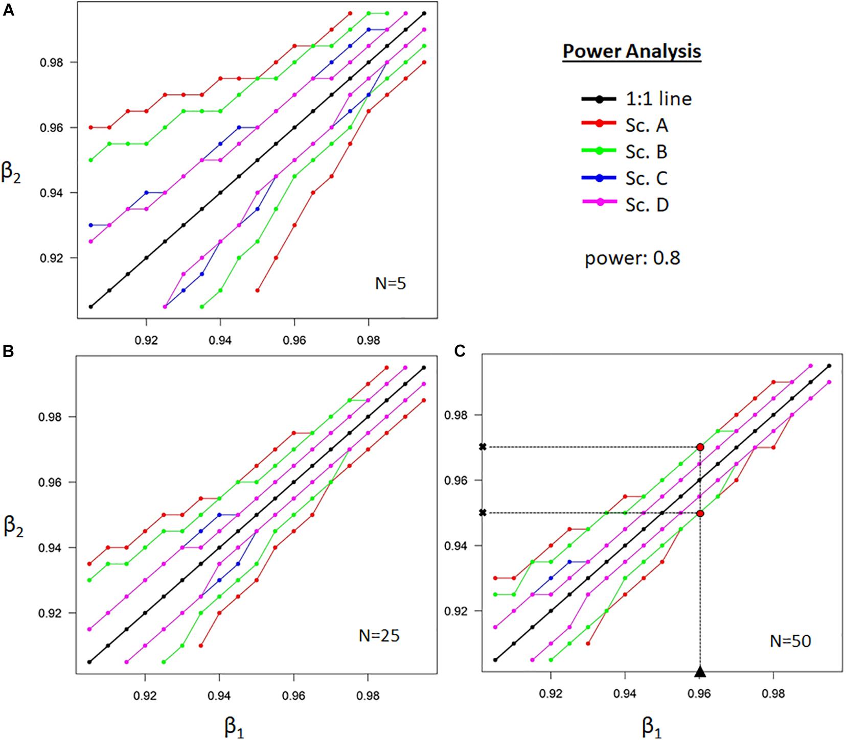
Figure 5. The power analysis shows the combinations of two allocation parameters that define the exponential vertical decay of the distribution of absorbing root surface with soil depth (β) of two independent datasets for a given sample size N, required to detect significant differences. Regions bounded by lines are non-significant (at the 95% level). The different colors correspond to four scenarios, as described in the main text and Figure 2. Panel (A–C), respectively show power analysis for sample sizes of 5, 25, and 50 samples. The level of confidence of finding significant differences, i.e., the power, is set at 0.8. An example is provided in (C) for a study case with β1 = 0.96, N = 50 and no restrictions (Sc A.). Significant differences can be expected with a power of 0.8 when the compared species has β-values outside the delineated range of both obtained β2-values.
Practical Case Study
We observed a shallower shape of the absorbing root surfaces distribution, i.e., smaller , for lianas (0.657, i.e., half of A_R in the upper 2 cm soil layer) than for their co-occurring trees (0.954, i.e., half of A_R in the upper 15 cm soil layer) (Figure 6; parameterization Supplementary Table 3). However, as setup A ignored all biophysical parameters, uncertainty in the estimates is much larger and showed a non-robust difference between lianas and trees (Figure 6A and Table 2). This considerable uncertainty resulted from the poor characterization of ΨS profile. Applying inverse SWIFT for scenario B, with field measurements of the ΨS, resulted in a much more conspicuously difference in mean δ2H for trees and lianas and a substantial reduction in uncertainty, i.e., an uncertainty range improvement of ∼ 4.0 (Figure 6 and Table 2). The latter highlights the uncertainty underestimation by De Deurwaerder et al. (2018), which used a standard approach due to unmeasured biophysical parameters.
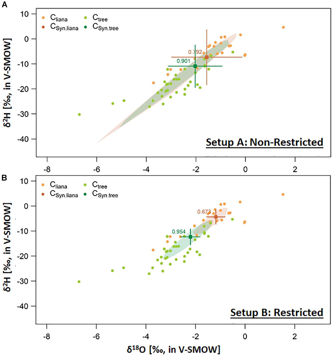
Figure 6. Dual isotope plot representation of the xylem water isotope compositions (δxyl) of trees (Ctree, ) and lianas (Cliana,
 ) obtained in Laussat, French Guiana, in 2017. Setup (A) Study setup which ignored restriction in soil water potential measurements, i.e., ΨS and Setup (B) Study setup with a more superior characterization of ΨS. Mean ± 2x standard error of simulated δxyl provided for the mean of 10 independent optimization assessments (i.e., ), provided for trees (CSyn.tree,
  ) and lianas (CSyn.liana,
  ). Corresponding convex hulls shows the pooled simulated δxyl range for all 10 independent optimizations. Applied parameterization is provided in Supplementary Table 3. Mean optimized values are provided in respective colors. Related standard error confidence intervals are provided in Table 2.
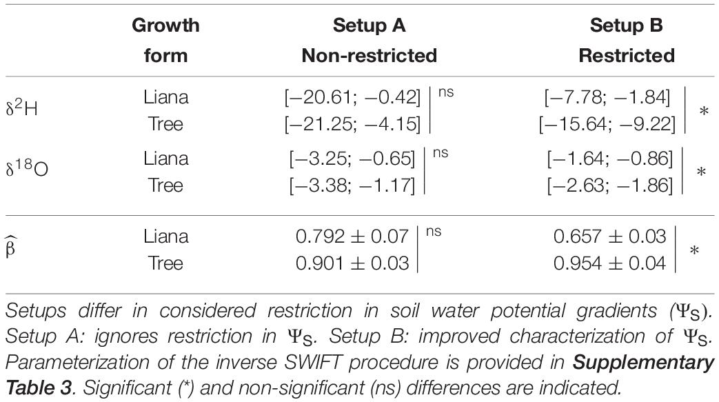
Table 2. The standard error confidence intervals (i.e., 2.5 and 97.5 percentiles) and corresponding mean (±1SD) of inverse SWIFT simulated conditional density probability distributions, i.e., P(), of xylem water isotope composition of lianas and trees for Laussat, French Guiana.
Discussion
This study introduces a parametric method to estimate AR with stable isotope data. The main benefit of the inverse SWIFT approach is that it provides a more realistic quantification of uncertainty, as well as improved accuracy (Figure 3). Simulations suggest that will likely be systematically overestimated and uncertainty considerably underestimated when ignoring field conditions. Both uncertainty and estimation bias can be significantly reduced by (1) improved characterization of soil heterogeneity (i.e., by accurate characterization of ΨS andδSoil) in combination with (2) optimized sampling that accounts for RWU and sap flow dynamics (De Deurwaerder et al., 2020). The former implies a study setup that monitors δSoil and ΨS in different soil layers and locations, and our simulation suggest that this should be prioritized above increasing the number of δxyl samples. The latter involves the application of a study design where sampling targets the δxyl corresponding to peak RWU, which results in a more pronounced V-shaped log-likelihood curve (Figure 2), i.e., less skewness inP(δxyl|β,χ) and hence far less uncertainty.
Case Study Findings
De Deurwaerder et al. (2018) reported significantly enriched δxyl for lianas compared to co-occurring trees during the dry season in Paracou (French Guiana) which suggests shallower root systems for lianas (as also shown elsewhere: Johnson et al., 2013; Carvalho et al., 2016; Smith-Martin et al., 2019, 2020). However, De Deurwaerder et al. (2018) approach ignored soil properties and many plant physiological processes that increase variance in δxyl. As our case study for Laussat shows, the lack of relevant biophysical information results in underestimating uncertainty in the mean δxyl. The latter implies that the findings of De Deurwaerder et al. (2018) can be explained by factors other than rooting depth, and should in hindsight have been interpreted with more caution than initially reported. Next, we applied an improved sampling setup in Laussat with a better representation of ΨS, which resulted in a strong drop in uncertainty and while still suggesting that a shallower absorbing root surface distribution for lianas is required to explain the differences in δxyl at least when only considering the confounders included in the current model (see “Recommendations and Future Directions” below). The results of these case study are also in line with our power analysis (Figure 5), which show that better quantification of ΨS should yield an improved ability to detect robust differences between these two growth forms. This highlights the importance of optimizing data collection and sampling strategy.
Recommendations and Future Directions
De Deurwaerder et al. (2020) showed that many biophysical variables could contribute to the intra-individual variance in δxyl. In the present study, we discussed how a power-analysis using mechanistic plant hydrological models could help optimize study designs and help restrict confounding parameters by identifying the most important biophysical variables to monitor. The latter could be invaluable to optimize sample sizes to maximize the efficient use of labor, resources, and time. Our simulations and analysis suggest that monitoring of soil heterogeneity (i.e., ΨS, δ18OS, and δ2HS profiles) and sap flow dynamics contribute to increased power in the detection of differences between plants in their distribution of absorbing root surfaces (A_R), especially when targeted sample sizes are small.
The use of stable water isotopes offers a scalable, time and labor efficient alternative for root excavation. When this is combined with models such as inverse SWIFT, we show that the A_R (as defined by β) can be assessed indirectly with high accuracy and power. This technique is not only unique in its ability to simultaneously assess A_R and RWU; but its less intrusive nature also supports repetitive sampling to study temporal dynamics. However, intra-individual variance in δxyl may be impacted by physiological plant processes or soil properties currently not considered. The robustness of the inverse approaches such as the one used here might therefore benefit from further improvements. The latter will require applying both (i) a more realistic modeling and improved theory; and (ii) more experimental and empirical work that monitors the impact of relevant physiological plant processes or soil properties on variance in δxyl. Essential considerations include temporal and spatial soil dynamics, fractionation at the root level, and storage tissue and phloem enrichment (see also De Deurwaerder et al., 2020).
Inverse SWIFT provides a robust tool to estimate β for plants which A_R approximates a power-law distribution. The latter is a basic representation of root systems in the current SWIFT model. A promising starting point for improvement would be the representation of roots to include more details as in models such as R-SWMS (Javaux et al., 2008) or SPACSYS (Wu et al., 2007). Such detail may be required to account for temporal and spatial soil and root dynamics properly, and in extension their impact on δxyl. Moreover, such approaches would support an improved representation of the flow path length within the rooting system allowing a more realistic propagation of isotopic composition from soil to the stem base (Seeger and Weiler, 2021).
The implementation of mycorrhizal colonization as an integral component of the water uptake process may present an additional perspective for future model improvement. While their direct contribution to RWU remains unclear (Ruth et al., 2011), various studies have highlighted an increased root hydraulic conductivity because of mycorrhizal colonization (Gianinazzi-Pearson and Gianinazzi, 1983; Augé, 2001; Aroca et al., 2007). Hence, as long as mycorrhizal colonization is relatively uniformly distributed over the rooting system, the impact of mycorrhizae on the inverse SWIFT assessment can be resolved indirectly by altering k_R. However, inverse SWIFT may become prone to biased assessment when colonization is not uniform and the proportional contribution of water influx via mycorrhizae is substantial. Indeed, future endeavors to implement a more dynamic AR and which can account for mycorrhizal colonization are encouraged.
Besides, many unknowns hamper model development. For instance, the extent to which fractionation during root water uptake or within the plant arises needs to be quantified before implementation. Here, root membrane (Lin and Sternberg, 1993; Zhao et al., 2016; Vargas et al., 2017) and mycorrhizal fractionation (Poca et al., 2019) present pathways that may introduce additional uncertainty. Also, stable water isotopes studies generally assume no alteration in δxyl once contained within the plant’s conduit system. We encourage evaluation of this assumption, as δxyl enrichment via storage tissue or phloem is not unreasonable (Barbeta et al., 2020; Knighton et al., 2020), which would pose additional model interpretation complexities.
Conclusion
Root excavation can only provide a snapshot, a one-time-only measure due to its destructive nature. A stable water isotopes approach is advantageous for upscaling root attributes in space and time. Stable water isotope approaches can be applied over a wide range of edaphic and environmental conditions (Zhao et al., 2016). New developments in high temporal resolution monitoring of xylem water isotope composition would enable quantification of absorbing root surfaces distributions over time. This all can provide invaluable insights for understanding drought strategy and water competition among different plant species. However, this exciting prospect is only possible when techniques are unbiased under different edaphic or physiological conditions between plant species and sites. Our work here highlights a key role for mechanistic inverse plant model to help guide the research agenda for the critical zone and water stable isotope work.
Data Availability Statement
The raw data supporting the conclusions of this article will be made available by the authors, upon reasonable request.
Author Contributions
HV, MV, and PB supervised and provided guidance throughout all aspects of the research. HD, MV, and MD designed the study. PH-F provided guidance and training in sample collection, processing, and interpretation. HD collected the samples and data during the field campaign and performed the processing and analysis of the samples. HD, MV, MD, and FM developed and coded the model. All authors contributed to the interpretation of the results and to the text of the manuscript.
Funding
This research was funded by the European Research Council Starting Grant 637643 (TREECLIMBERS), the Carbon Mitigation Initiative at Princeton University (HD, MD, and MV), Agence Nationale de la Recherche “Investissement d’Avenir” grant (CEBA: ANR-10-LABX-25-01), the FWO grants (1214720N to FM and V401018N to HD), the Belgian American Educational Foundation (BAEF to HD and FM), and WBI to FM. The Programa de Formación de Personal Avanzado CONICYT, BECAS CHILE (PH-F) and the Commissie Wetenschappelijk Onderzoek (CWO, Faculty of Bioscience Engineering to PH-F).
Conflict of Interest
The authors declare that the research was conducted in the absence of any commercial or financial relationships that could be construed as a potential conflict of interest.
Acknowledgments
We thank Dries Van Der Heyden, Wim Van Nunen, Laurence Stalmans, Oscar Vercleyen, Katja Van Nieuland, Stijn Vandevoorde, and Clément Stahl for data collection and lab processing. We thank two reviewers and editor for their constructive comments on the manuscript. We are grateful to Cora N. Betsinger for proofreading and Kathy Steppe, Mathieu Javaux, Frank Sterck, Jan Van den Bulcke, and Stephen W. Pacala for insightful discussions.
Supplementary Material
The Supplementary Material for this article can be found online at: https://www.frontiersin.org/articles/10.3389/ffgc.2021.689335/full#supplementary-material
References
Allison, G. B., Barnes, C. J., Hughes, M. W., and Leaney, F. W. J. (1983). Effect of climate and vegetation on oxygen-18 and deuterium profiles in soils. Isotope Hydrol. 105–123.
Araguás-Araguás, L., Rozanski, K., Gonfiantini, R., and Louvat, D. (1995). Isotope effects accompanying vacuum extraction of soil water for stable isotope analyses. J. Hydrol. 168, 159–171. doi: 10.1016/0022-1694(94)02636-p
Araguás-Araguás, L., Froehlich, K., and Rozanski, K. (1998). Stable isotope composition of precipitation over southeast Asia. J. Geophys. Res. 103, 28721–28742. doi: 10.1029/98jd02582
Aroca, R., Porcel, R., and Ruiz-Lozano, J. M. (2007). How does arbuscular mycorrhizal symbiosis regulate root hydraulic properties and plasma membrane aquaporins in Phaseolus vulgaris under drought, cold or salinity stresses? N. Phytol. 173, 808–816. doi: 10.1111/j.1469-8137.2006.01961.x
Augé, R. M. (2001). Water relations, drought and vesicular-arbuscular mycorrhizal symbiosis. Mycorrhiza 11, 3–42. doi: 10.1007/s005720100097
Baraloto, C., Rabaud, S., Molto, Q., Blanc, L., Fortunel, C., Herault, B., et al. (2011). Disentangling stand and environmental correlates of aboveground biomass in Amazonian forests. Glob. Change Biol. 17, 2677–2688. doi: 10.1111/j.1365-2486.2011.02432.x
Barbeta, A., Gimeno, T. E., Clavé, L., Fréjaville, B., Jones, S. P., Delvigne, C., et al. (2020). An explanation for the isotopic offset between soil and stem water in a temperate tree species. N. Phytol. 227, 766–779. doi: 10.1111/nph.16564
Barbeta, A., Jones, S. P., Clavé, L., Wingate, L., Gimeno, T. E., Fréjaville, B., et al. (2019). Unexplained hydrogen isotope offsets complicate the identification and quantification of tree water sources in a riparian forest. Hydrol. Earth Syst. Sci. 23, 2129–2146. doi: 10.5194/hess-23-2129-2019
Beyer, M., Hamutoko, J. T., Wanke, H., Gaj, M., and Koeniger, P. (2018). Examination of deep root water uptake using anomalies of soil water stable isotopes, depth-controlled isotopic labeling and mixing models. J. Hydrol. 566, 122–136. doi: 10.1016/j.jhydrol.2018.08.060
Cabal, C., De Deurwaerder, H. P. T., and Matesanz, S. (2021). Field methods to study the spatial root density distribution of individual plants. Plant Soil 462, 1–19.
Carvalho, E. C. D., Martins, F. R., Oliveira, R. S., Soares, A. A., and Araújo, F. S. (2016). Why is liana abundance low in semiarid climates? Austral. Ecol. 41, 559–571. doi: 10.1111/aec.12345
Čermák, J., Ulrich, R., Staněk, Z., Koller, J., and Aubrecht, L. (2006). Electrical measurement of tree root absorbing surfaces by the earth impedance method: 2. Verification based on allometric relationships and root severing experiments. Tree Physiol. 26, 1113–1121. doi: 10.1093/treephys/26.9.1113
Chen, Y., Cao, K., Schnitzer, S. A., Fan, Z., Zhang, J., Bongers, F., et al. (2015). Water-use advantage for lianas over trees in tropical seasonal forests. N. Phytol. 205, 128–136. doi: 10.1111/nph.13036
Chen, Y., Helliker, B. R., Tang, X., Li, F., Zhou, Y., and Song, X. (2020). Stem water cryogenic extraction biases estimation in deuterium isotope composition of plant source water. Proc. Natl. Acad. Sci. U. S. A. 117, 33345–33350. doi: 10.1073/pnas.2014422117
Chen, Y., Schnitzer, S. A., Zhang, Y., Fan, Z., Goldstein, G., Tomlinson, K. W., et al. (2017). Physiological regulation and efficient xylem water transport regulate diurnal water and carbon balances of tropical lianas. Funct. Ecol. 31, 306–317. doi: 10.1111/1365-2435.12724
Clapp, R. B., and Hornberger, G. M. (1978). Empirical equations for some soil hydraulic properties. Water Resour. Res. 14, 601–604. doi: 10.1029/wr014i004p00601
Craig, H. (1961). Isotopic variations in meteoric waters. Science 133, 1702–1703. doi: 10.1126/science.133.3465.1702
Cristiano, P. M., Campanello, P. I., Bucci, S. J., Rodriguez, S. A., Lezcano, O. A., Scholz, F. G., et al. (2015). Evapotranspiration of subtropical forests and tree plantations: A comparative analysis at different temporal and spatial scales. Agricult. Forest Meteorol. 203, 96–106. doi: 10.1016/j.agrformet.2015.01.007
Dawson, T. E., and Ehleringer, J. R. (1991). Streamside trees that do not use stream water. Nature 350, 335–337. doi: 10.1038/350335a0
Dawson, T. E., Mambelli, S., Plamboeck, A. H., Templer, P. H., and Tu, K. P. (2002). Stable isotopes in plant ecology. Annu. Rev. Ecol. Syst. 33, 507–559.
De Deurwaerder, H., Hervé-Fernández, P., Stahl, C., Burban, B., Petronelli, P., Hoffman, B., et al. (2018). Liana and tree below-ground water competition—evidence for water resource partitioning during the dry season. Tree Physiol. 38, 1071–1083. doi: 10.1093/treephys/tpy002
De Deurwaerder, H. P. T., Visser, M. D., Detto, M., Boeckx, P., Meunier, F., Kuehnhammer, K., et al. (2020). Causes and consequences of pronounced variation in the isotope composition of plant xylem water. Biogeosciences 17, 4853–4870. doi: 10.5194/bg-17-4853-2020
Duong, T. (2007). ks: Kernel density estimation and kernel discriminant analysis for multivariate data in R. J. Stat. Softw. 21, 1–16.
Ehleringer, J. R., and Dawson, T. E. (1992). Water uptake by plants: perspectives from stable isotope composition. Plant Cell Environ. 15, 1073–1082. doi: 10.1111/j.1365-3040.1992.tb01657.x
Fogel, R. (1985). Roots as primary producers in below-ground ecosystems. FAO Rome: World Soil Resources.
Gaines, K. P., Meinzer, F. C., Duffy, C. J., Thomas, E. M., and Eissenstat, D. M. (2016). Rapid tree water transport and residence times in a Pennsylvania catchment. Ecohydrology 9, 1554–1565. doi: 10.1002/eco.1747
Gehring, C., Park, S., and Denich, M. (2004). Liana allometric biomass equations for Amazonian primary and secondary forest. Forest Ecol. Manag. 195, 69–83. doi: 10.1016/j.foreco.2004.02.054
Gerolamo, C. S., and Angyalossy, V. (2017). Wood anatomy and conductivity in lianas, shrubs and trees of Bignoniaceae. IAWA J. 38, 412–432. doi: 10.1163/22941932-20170177
Gerwing, J. J., Schnitzer, S. A., Burnham, R. J., Bongers, F., Chave, J., DeWalt, S. J., et al. (2006). A standard protocol for liana censuses. Biotropica 38, 256–261.
Gianinazzi-Pearson, V., and Gianinazzi, S. (1983). The physiology of vesicular-arbuscular mycorrhizal roots. Plant Soil 71, 197–209. doi: 10.1007/978-94-009-6833-2_20
Gibson, J. J., Birks, S. J., and Edwards, T. W. D. (2008). Global prediction of δA and δ2H-δ18O evaporation slopes for lakes and soil water accounting for seasonality. Glob. Biogeochem. Cycles 22:GB2031.
Gourlet-Fleury, S., Guehl, J. M., and Laroussinie, O. (2004). Ecology and Management of a Neotropical Rainforest: Lessons Drawn From Paracou, a Long-Term Experimental Research Site in French Guiana. New York: Elsevier.
Gröning, M. (2011). Improved water δ2H and δ18O calibration and calculation of measurement uncertainty using a simple software tool. Rap. Commun. Mass Spectr. 25, 2711–2720. doi: 10.1002/rcm.5074
Huang, C., Domec, J., Ward, E. J., Duman, T., Manoli, G., Parolari, A. J., et al. (2017). The effect of plant water storage on water fluxes within the coupled soil–plant system. New Phytol. 213, 1093–1106. doi: 10.1111/nph.14273
Iversen, C. M., Powell, A. S., McCormack, M. L., Blackwood, C. B., Freschet, G. T., Kattge, J., et al. (2018). Fine-Root Ecology Database (FRED): A Global Collection of Root Trait Data with Coincident Site, Vegetation, Edaphic, and Climatic Data, Version 2. Oak Ridge: Oak Ridge National Lab.(ORNL).
Jackson, R. B., Canadell, J., Ehleringer, J. R., Mooney, H. A., Sala, O. E., and Schulze. (1996). A global analysis of root distributions for terrestrial biomes. Oecologia 108, 389–411. doi: 10.1007/bf00333714
Javaux, M., Schröder, T., Vanderborght, J., and Vereecken, H. (2008). Use of a three-dimensional detailed modeling approach for predicting root water uptake. Vadose Zone J. 7, 1079–1088. doi: 10.2136/vzj2007.0115
Jobbagy, E. G., and Jackson, R. B. (2001). The distribution of soil nutrients with depth: Global patterns and the imprint of plants. Biogeochemistry 53, 51–77.
Johnson, D. M., Domec, J.-C., Woodruff, D. R., McCulloh, K. A., and Meinzer, F. C. (2013). Contrasting hydraulic strategies in two tropical lianas and their host trees. Am. J. Bot. 100, 374–383. doi: 10.3732/ajb.1200590
De Jong, van Lier, Q., Van Dam, J. C., Metselaar, K., De Jong, R., and Duijnisveld, W. H. M. (2008). Macroscopic root water uptake distribution using a matric flux potential approach. Vadose Zone J. 7, 1065–1078. doi: 10.2136/vzj2007.0083
Knighton, J., Kuppel, S., Smith, A., Soulsby, C., Sprenger, M., and Tetzlaff, D. (2020). Using isotopes to incorporate tree water storage and mixing dynamics into a distributed ecohydrologic modelling framework. Ecohydrology 13:e2201.
Leuschner, C., Coners, H., and Icke, R. (2004). In situ measurement of water absorption by fine roots of three temperate trees: species differences and differential activity of superficial and deep roots. Tree Physiol. 24, 1359–1367. doi: 10.1093/treephys/24.12.1359
Lin, G., and Sternberg, L. (1993). “Hydrogen isotopic fractionation by plant roots during water uptake in coastal wetland plants,” in Stable isotopes and plant carbon-water relations, eds J. R. Ehleringer, A. E. Hall, and G. D. Farquhar (Netherland: Elsevier), 497–510. doi: 10.1016/b978-0-08-091801-3.50041-6
Magh, R.-K., Eiferle, C., Burzlaff, T., Dannenmann, M., Rennenberg, H., and Dubbert, M. (2020). Competition for water rather than facilitation in mixed beech-fir forests after drying-wetting cycle. J. Hydrol. 587:124944. doi: 10.1016/j.jhydrol.2020.124944
Marshall, J. D., Cuntz, M., Beyer, M., Dubbert, M., and Kuehnhammer, K. (2020). Borehole equilibration: testing a new method to monitor the isotopic composition of tree xylem water in situ. Front. Plant Sci. 11:358. doi: 10.3389/fpls.2020.00358
Martin-Gomez, P., Barbeta, A., Voltas, J., Penuelas, J., Dennis, K., Palacio, S., et al. (2015). Isotope-ratio infrared spectroscopy: a reliable tool for the investigation of plant-water sources? N. Phytol. 207, 914–927. doi: 10.1111/nph.13376
Meinzer, F. C., Brooks, J. R., Domec, J., Gartner, B. L., Warren, J. M., Woodruff, D. R., et al. (2006). Dynamics of water transport and storage in conifers studied with deuterium and heat tracing techniques. Plant Cell Environ. 29, 105–114. doi: 10.1111/j.1365-3040.2005.01404.x
Meinzer, F. C., Goldstein, G., and Andrade, J. L. (2001). Regulation of water flux through tropical forest canopy trees: do universal rules apply? Tree Physiol. 21, 19–26. doi: 10.1093/treephys/21.1.19
Meißner, M., Köhler, M., Schwendenmann, L., and Hölscher, D. (2012). Partitioning of soil water among canopy trees during a soil desiccation period in a temperate mixed forest. Biogeosciences 9, 3465–3474. doi: 10.5194/bg-9-3465-2012
Mennekes, D., Rinderer, M., Seeger, S., and Orlowski, N. (2021). Ecohydrological travel times derived from in situ stable water isotope measurements in trees during a semi–controlled pot experiment. Hydrol. Earth Syst. Sci. Discuss. 2021, 1–34. doi: 10.1046/j.1440-1703.1998.00240.x
Orlowski, N., Frede, H. G., Brüggemann, N., and Breuer, L. (2013). Validation and application of a cryogenic vacuum extraction system for soil and plant water extraction for isotope analysis. J. Sens. Sens. Syst. 2, 179–193. doi: 10.5194/jsss-2-179-2013
Penna, D., Hopp, L., Scandellari, F., Allen, S. T., Benettin, P., Beyer, M., et al. (2018). Ideas and perspectives: Tracing terrestrial ecosystem water fluxes using hydrogen and oxygen stable isotopes–challenges and opportunities from an interdisciplinary perspective. Biogeosciences 15, 6399–6415. doi: 10.5194/bg-15-6399-2018
Phillips, D. L., and Gregg, J. W. (2003). Source partitioning using stable isotopes: coping with too many sources. Oecologia 136, 261–269. doi: 10.1007/s00442-003-1218-3
Poca, M., Coomans, O., Urcelay, C., Zeballos, S. R., Bodé, S., and Boeckx, P. (2019). Isotope fractionation during root water uptake by Acacia caven is enhanced by arbuscular mycorrhizas. Plant Soil 441, 1–13.
Preston, R. J. (1942). The growth and development of the root systems of juvenile lodgepole pine. Ecol. Monogr. 12, 449–468. doi: 10.2307/1943040
Rothfuss, Y., and Javaux, M. (2017). Reviews and syntheses: Isotopic approaches to quantify root water uptake: a review and comparison of methods. Biogeosciences 14:2199. doi: 10.5194/bg-14-2199-2017
Rozanski, K., Araguás-Araguás, L., and Gonfiantini, R. (1993). Isotopic patterns in modern global precipitation. Clim. Change Cont. Isot. Rec. 1993, 1–36. doi: 10.1029/gm078p0001
Rüdinger, M., Hallgren, S. W., Steudle, E., and Schulze, E.-D. (1994). Hydraulic and osmotic properties of spruce roots. J. Exp. Bot. 45, 1413–1425. doi: 10.1093/jxb/45.10.1413
Ruth, B., Khalvati, M., and Schmidhalter, U. (2011). Quantification of mycorrhizal water uptake via high-resolution on-line water content sensors. Plant Soil 342, 459–468. doi: 10.1007/s11104-010-0709-3
Sands, R., Fiscus, E. L., and Reid, C. P. P. (1982). Hydraulic properties of pine and bean roots with varying degrees of suberization, vascular differentiation and mycorrhizal infection. Funct. Plant Biol. 9, 559–569. doi: 10.1071/pp9820559
Seeger, S., and Weiler, M. (2021). Temporal dynamics of tree xylem water isotopes: In-situ monitoring and modelling. Biogeosciences Discuss. 2021, 1–41.
Smith-Martin, C. M., Bastos, C. L., Lopez, O. R., Powers, J. S., and Schnitzer, S. A. (2019). Effects of dry-season irrigation on leaf physiology and biomass allocation in tropical lianas and trees. Ecology 100:e02827.
Smith-Martin, C. M., Xu, X., Medvigy, D., Schnitzer, S. A., and Powers, J. S. (2020). Allometric scaling laws linking biomass and rooting depth vary across ontogeny and functional groups in tropical dry forest lianas and trees. New Phytol. 226, 714–726. doi: 10.1111/nph.16275
Soethe, N., Lehmann, J., and Engels, C. (2006). The vertical pattern of rooting and nutrient uptake at different altitudes of a south Ecuadorian montane forest. Plant Soil 286, 287–299. doi: 10.1007/s11104-006-9044-0
Steudle, E., and Meshcheryakov, A. B. (1996). Hydraulic and osmotic properties of oak roots. J. Exp. Bot. 47, 387–401. doi: 10.1093/jxb/47.3.387
Vargas, A. I., Schaffer, B., Yuhong, L., Sternberg, L., and da, S. L. (2017). Testing plant use of mobile vs immobile soil water sources using stable isotope experiments. New Phytol. 215, 582–594. doi: 10.1111/nph.14616
Vogel, T., Dohnal, M., Dusek, J., Votrubova, J., and Tesar, M. (2013). Macroscopic modeling of plant water uptake in a forest stand involving root-mediated soil water redistribution. Vadose Zone J. 12, 1–12.
von Freyberg, J., Allen, S. T., Grossiord, C., and Dawson, T. E. (2020). Plant and root-zone water isotopes are difficult to measure, explain, and predict: Some practical recommendations for determining plant water sources. Methods Ecol. Evolut. 11, 1352–1367. doi: 10.1111/2041-210x.13461
Walker, C. D., and Richardson, S. B. (1991). The use of stable isotopes of water in characterizing the source of water in vegetation. Chem. Geol. 94, 145–158. doi: 10.1016/0168-9622(91)90007-j
Wershaw, R. L., Friedman, I., Heller, S. J., and Frank, P. A. (1966). Hydrogen isotopic fractionation of water passing through trees. Adv. Organic Geochem. 118, 55–67. doi: 10.1016/b978-0-08-012758-3.50007-4
White, J. W. C., Cook, E. R., Lawrence, J. R., and Broecker, W. S. (1985). The D/H ratios of sap in trees - implications for water sources and tree-ring D/H ratios. Geochim. Cosmochim. Acta 49, 237–246. doi: 10.1016/0016-7037(85)90207-8
Wu, L., McGechan, M. B., McRoberts, N., Baddeley, J. A., and Watson, C. A. (2007). SPACSYS: integration of a 3D root architecture component to carbon, nitrogen and water cycling—model description. Ecol. Model. 200, 343–359. doi: 10.1016/j.ecolmodel.2006.08.010
Zanne, A. E., Westoby, M., Falster, D. S., Ackerly, D. D., Loarie, S. R., Arnold, S. E. J., et al. (2010). Angiosperm wood structure: global patterns in vessel anatomy and their relation to wood density and potential conductivity. Am. J. Bot. 97, 207–215. doi: 10.3732/ajb.0900178
Zhao, L., Wang, L., Cernusak, L. A., Liu, X., Xiao, H., Zhou, M., et al. (2016). Significant difference in hydrogen isotope composition between xylem and tissue water in Populus euphratica. Plant Cell Environ. 39, 1848–1857. doi: 10.1111/pce.12753
Keywords: absorbing root surfaces distribution, ecohydrology, lianas, stable water isotopes, tropical trees, water competition
Citation: De Deurwaerder HPT, Visser MD, Meunier F, Detto M, Hervé-Fernández P, Boeckx P and Verbeeck H (2021) Robust Estimation of Absorbing Root Surface Distributions From Xylem Water Isotope Compositions With an Inverse Plant Hydraulic Model. Front. For. Glob. Change 4:689335. doi: 10.3389/ffgc.2021.689335
Received: 31 March 2021; Accepted: 01 June 2021;
Published: 12 July 2021.
Edited by:
Yuanyuan Huang, Climate Science Centre, CSIRO Oceans and Atmosphere, AustraliaReviewed by:
Alan Feest, University of Bristol, United KingdomXiaochi Ma, University of California, Davis, United States
Copyright © 2021 De Deurwaerder, Visser, Meunier, Detto, Hervé-Fernández, Boeckx and Verbeeck. This is an open-access article distributed under the terms of the Creative Commons Attribution License (CC BY). The use, distribution or reproduction in other forums is permitted, provided the original author(s) and the copyright owner(s) are credited and that the original publication in this journal is cited, in accordance with accepted academic practice. No use, distribution or reproduction is permitted which does not comply with these terms.
*Correspondence: Hannes P. T. De Deurwaerder, SGFubmVzX2RlX2RldXJ3YWVyZGVyQGhvdG1haWwuY29t