Abstract
A rapid, reliable, cost-effective tree volume calculation is critical for estimating biomass and carbon sequestration. This estimation is vital for developing better carbon budgets for wetland ecosystems to assess current and future climate scenarios. Portable mobile light detection and ranging (LiDAR) systems such as the Apple iPad Pro sensor provide an efficient method for capturing 3D shapes of bald cypress (Taxodium distichum) pneumatophores, or “knees.” The knee is a rounded conical structure growing above the water or land from the roots of bald cypress trees, usually a few feet away from the trunk. This study explores remote sensing techniques for mapping individual knees to eventually understand their significance in the carbon balance of forested wetlands. This project was conducted in the Three Sisters Swamp, part of the Black River Reserve in North Carolina, USA. The volume of individual tree knees was estimated using multiple geometric algorithms and compared to allometric estimates from traditional field measurements derived from the shape of a cone. Specifically, we used the convex-hull by slicing (C-hbS) and Canopy-Surface Height (CSH) algorithms to estimate the volume of individual knees after LiDAR data processing. The volume estimates from the CSH and C-hbS methods are higher than the allometric estimates due to the knees’ natural irregular shape and concavities. The CSH method returned the largest volume values on average. The discrepancy in estimated volume between the allometric equation and the two algorithms became more pronounced with increasing knee height. The estimated aboveground mean biomass and carbon of the knees are 61.9 ± 23.4 Mg ha−1 and 32.83 ± 12.38 Mg C ha−1, respectively. The challenges of algorithmic methods include the time and equipment needed to process dense point clouds. However, they better capture irregularities in knee shape, ultimately leading to better estimates and an understanding of knee structure, which is currently poorly understood.
1 Introduction
Examining carbon sequestration in wetlands is important for developing carbon budgets, which are needed to understand wetlands’ role in the global carbon cycle (Bridgham et al., 2006). Estimating the amount of forest biomass is critical and essential for calculating biomass energy, carbon storage, and sequestration of carbon in a forested ecosystem (Hossain et al., 2015; Vashum and Jayakumar, 2012), as well as for studying climate change, forest health, ecosystem productivity, and nutrient cycling (Dong et al., 2014). An accurate calculation of tree volume is needed to determine biomass estimates. This volume can be converted into dry weight using the wood density factor to predict the forest’s total biomass and carbon storage (Demol et al., 2022; Sagang et al., 2018; Yusup et al., 2023).
The bald cypress tree (Taxodium distichum) has been observed to tolerate flooded conditions for extended periods (Meyer, 2020). Cypress trees provide excellent flood control by absorbing surface water runoff over the short term, especially during storms (Parresol, 2002). The water absorbed during the rainy season can replenish the depleted water table during the dry season. It also serves as a habitat and breeding ground for wildlife and rare species, and it minimizes disturbance from gale and hurricane-force winds (Parresol, 2002; Wilhite and Toliver, 1990).
One of the distinct features of bald cypress is the woody protrusions of pneumatophores, or knees, growing from its root system (Lamborn, 1890). Carbon stock trends of the knees of bald cypress vary across climate gradients in the southeastern United States (Middleton, 2020). Hence, the knees contribute an unknown quantity of “teal” carbon to inland freshwater wetlands (Middleton, 2020). Teal carbon is the term used to describe the carbon stored in inland freshwater wetlands (Nahlik and Fennessy, 2016). The cypress knees often have swollen bases or buttresses (Briand, 2021), and the woody conical structures of varying sizes are found around the base of many cypress tree stems (see Figure 1A).
Figure 1
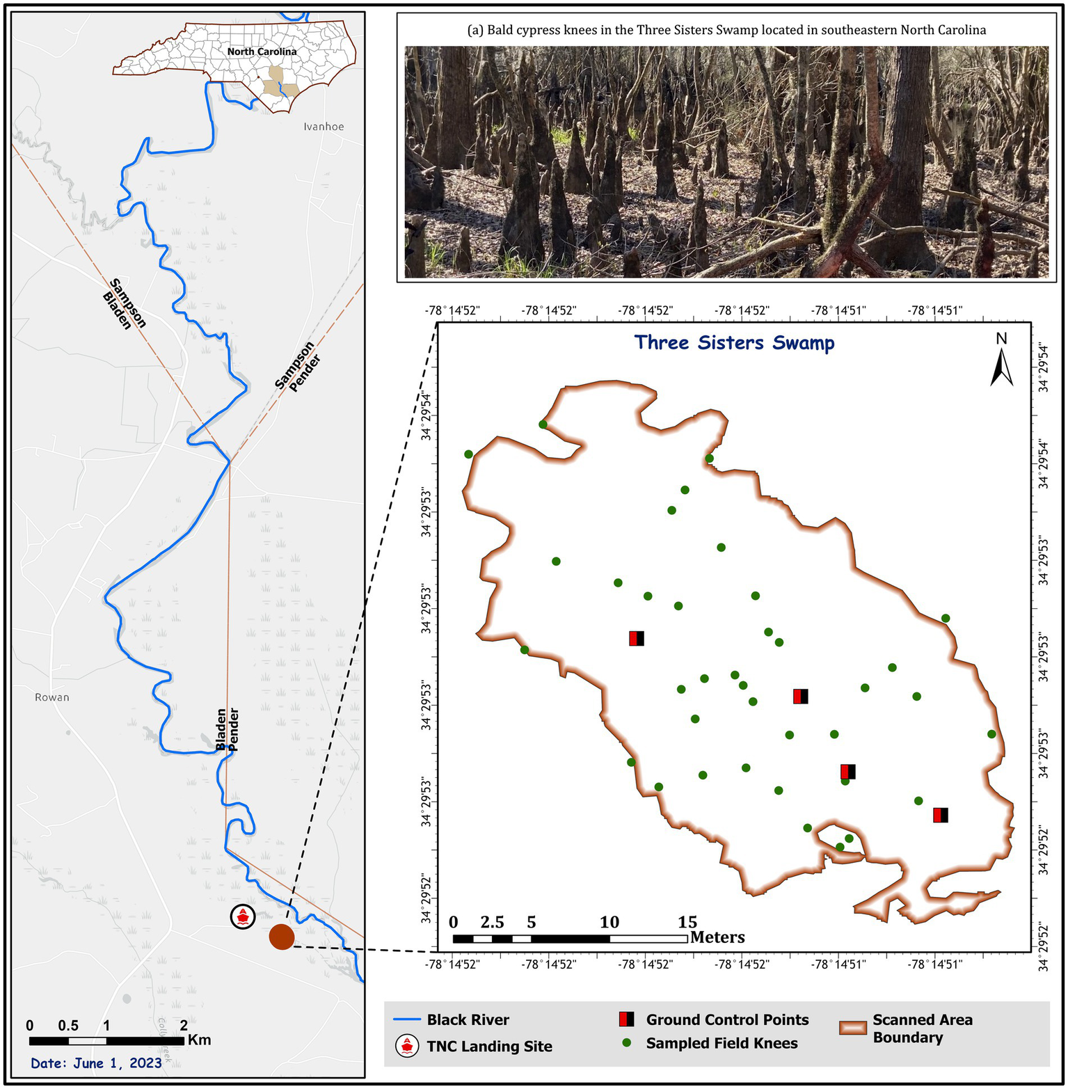
Map of the study area with the boundary indicated in brown, ground control points identified with squares, and the field sampled knees identified with circles.
On an ecosystem level, these knees are thought to play a substantial role in carbon storage by contributing between 5.2 and 17% of the overall carbon stored in the Mississippi River Alluvial Valley (Ketterings et al., 2001; Middleton, 2020). While a standard, accepted, and commonly used allometric equation for carbon assessments would be valuable, knees vary significantly in size (Brown, 1984), so a single value representing this species’ carbon contribution may be impossible (Middleton, 2020). If the amounts of knee carbon are sizable in various swamp environments, a non-destructive technique could be a very useful tool for estimating the carbon contribution of these forests to global stocks (Middleton, 2020).
Previous studies have employed a traditional approach to estimating the volume and biomass of cypress knees (Middleton, 2020) using allometric equations that approximate the knee shape or form to a geometric cone. Measuring forest biomass through field surveys at a large spatial scale is time-consuming and costly (Hermosilla et al., 2014; van Leeuwen and Nieuwenhuis, 2010). Remote sensing technology, such as Light Detection and Ranging (LiDAR), has proved its potential to provide detailed forest canopy characteristics (Cao et al., 2016). Individual tree height with sub-meter vertical precision can be extracted from LiDAR data, from which diameter estimates can be predicted; both metrics have significant advantages in forest aboveground biomass (AGB) estimation (Cao et al., 2016; Hudak et al., 2012; Lu et al., 2020). The choice of techniques for volume and biomass estimation depends on various factors (Shi and Liu, 2017), namely the ecosystem being studied, the species or object of interest, the aim of the study, the level of detail needed in terms of resolution and scale, and the cost. Fernández-Sarría et al. (2013) estimated individual tree (P. hispanica) volume and biomass from terrestrial laser point clouds and ground-level measurements using four different methods: convex-hull, convex-hull by slices, triangulation, and voxel modeling. Vauhkonen et al. (2012) extracted canopy volume based on Airborne Laser Scanning (ALS) data using a 3-dimensional (3D) alpha-shape algorithm. Korhonen et al. (2013) used 3D alpha shape and 3D convex hull techniques to extract tree crown volumes from ALS data, with the results showing that the LiDAR-based estimates were highly correlated with the field-measured tree crown volumes (best R2 = 0.83) and the convex-hull techniques producing the best accuracy. However, one of the drawbacks of the convex-hull estimation is overestimation of crown volume due to inability to account for gaps with the crown structure (Kato et al., 2009; Korhonen et al., 2013).
On the other hand, Chang et al. (2017) estimated the volume of objects from a 3D point cloud by cutting them into slices of equal thickness along the z-axis, bisecting each slice along the y-axis, and integrating the slices to estimate area and volume. Zhi et al. (2016) calculated the volume of a 3D point cloud based on the slice method where the object was sliced along the z-axis, and each slice was projected onto the x-y plane; the area was then estimated using Euclidean geometry and volume by multiplying each projected surface area by the height of the slice. Combining the slice-based volume techniques with the 3D convex hull (Fernández-Sarría et al., 2013) shows that convex-hull by slices reduces error in the tree crown volume compared to the 3D convex hulls without slicing and voxel method. Furthermore, Yan et al. (2019) also showed that a slicing-based method adapted to the tree crown change rates along the vertical direction enhances volume accuracy by aligning the number of slices and thickness to the shape and size of the tree crown. To our knowledge, no study has examined these approaches to estimate the biomass of cypress knees.
A combination of platforms and techniques can accurately estimate volume extent and biomass (Swetnam et al., 2018). Remote sensing, calibrated by field measurements, addresses these challenges and limitations (Gonzalez et al., 2010). Portable scanning LiDAR systems can capture individual trees’ complex shapes and structures as a detailed 3-D point-cloud image (Hosoi et al., 2013). We explored methods for estimating the volume of bald cypress knees using a LiDAR sensor of an Apple iPad Pro. We compared the estimates of the convex-hull by slicing (C-hbS) and Canopy Surface Height (CSH)--based algorithms to those obtained from an allometric equation and field measurements. Our study aims to fill a gap in the knowledge of the volume and structure of cypress knees and highlight the ecological importance of one of the oldest cypress groves in North America, found in the Black River Reserve.
2 Materials and methods
2.1 Study area
The Black River is a nutrient-poor blackwater tributary of the Cape Fear River, approximately 50 miles long, in southeastern North Carolina in the United States (Stahle et al., 1988). As its name suggests, the Black River is a slow-moving river within the Blackwater system in southern Sampson County (Figure 1). The Black River flows through Bladen County southeast toward Pender County, where it joins the Cape Fear River (Library of Congress, 2015). A blackwater river is a system with slow-moving waterways flowing through forested wetlands or swamps. As vegetation decays, tannins leach into the water, making transparent, acidic, darkly stained water resembling black tea (Janzen, 1974). It is more acidic than other freshwater ecosystems because of vegetation decay and the subsequent release of tannins in the water. The nature of this environment makes it unfavorable for many hardwood tree species and slows down the growth of bald cypress (Stahle et al., 2019).
The climate of the Black River area is characterized by inter-annual variability in water levels, intense evapotranspiration demand during the growing seasons, and frequently flooded conditions that prevail in the forested wetlands in the Southeastern United States (Davidson and Janssens, 2006; Stahle et al., 2012). Water levels fluctuate significantly throughout the year, with an average water depth of 1.2 meters (m), and the river is, on average, 45.7 m wide (North Carolina Division of Parks and Recreation (NCDPR), 2018). The highest flow occurs during winter and early spring. While summer and fall have somewhat lower flows, flow during the dry months is augmented and sustained to some extent by the water stored underground and the water held in swamps (Bureau of Outdoor Recreation, 1971).
The Black River is home to a grove of old-growth cypress trees, some more than 1,700 years old (Stahle et al., 1988). Recent research shows that the forested wetlands of the Black River preserve one of the oldest living bald cypress trees in southeastern North Carolina at 2,624 years old (Stahle et al., 2019). During dry periods, especially throughout the summer, fallen logs in the river make maneuvering the river difficult (Taylor, 2005). Our study site is located along the Black River at the Three Sister Swamp in Bladen County (Figure 1). The swamp is approximately 1.6 kilometers (km) long and 0.8 km wide, serving as home to the largest cluster of ancient cypress trees in the entire Black River Preserve (Horan, 2020). We accessed the study area by launching kayaks from the Nature Conservancy (TNC) landing site. The area sampled in this study is relatively small, given the complex nature of the ecosystems.
2.2 Data collection
2.2.1 Field data
We randomly selected 55 knees for measurement in the field on May 24, 2023. For each knee, we measured the diameter at water level or ground and the slant height, defined as the base to the apex for the longest side (Figure 2). Given the conical and irregular shape of the knee, actual height cannot be directly measured. It took an average of 35 s for two people and an average of 80 s for a single person to measure an individual knee, including recording the data.
Figure 2
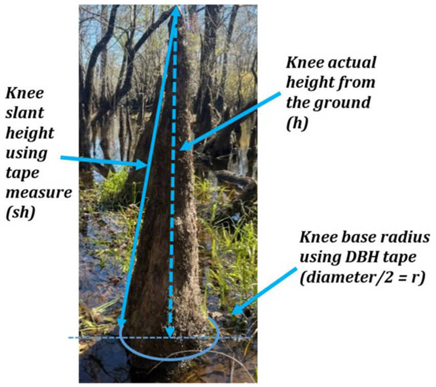
Field measurements of an individual knee. The slant height was taken along the longest external line of the knee from the ground to the tip, the radius of the knee was measured at the ground, and the actual height was estimated from these two values.
We calculated the actual height in cm Equation 1, from tip (apex) to ground or water line using Pythagoras’ theorem:
The volume in cm3 was calculated using the equation for a cone Equation 2. Middleton (2020) has used this equation for cypress knees in Florida:
Based on the field metrics, we found that the minimum radius was 4.6 cm, and the maximum was 25.3 cm, with an average of 13.3 cm. The minimum and maximum heights were 30.14 cm and 201.7 cm, respectively, with an average value of 85.7 cm.
Additionally, oven-dry weight refers to the weight of the wood materials after completely drying in an oven. To estimate the wood density needed for the computation of biomass, we randomly selected and cored 15 knees of varying sizes. We placed the harvested knee cores in the oven for about 4 days and heated them at a 120-degree temperature to remove all the moisture. We calculated the volume (cm3) of each core, measured the weight of the dried wood cores [i.e., mass (g)], and calculated the wood density (g/cm3) as follows Equation 3:
2.2.2 LiDAR data
The Apple iPad Pro 12.9″, 256 GB (Apple Inc., Cupertino, CA, USA) running iOS 14.6 has an integrated LiDAR sensor that provides cost-effective alternatives to established techniques in remote sensing with possible field applications (Luetzenburg et al., 2021). This hand-held mobile device includes a LiDAR module on the rear camera cluster, which includes the receptor and emitter (Yoshida, 2020). We used this device to derive the 3D point clouds of the knees in the Three Sisters Swamp. We covered an area of 822.1 square meters (m2) from three different area scans on May 24, 2023. We performed three non-overlapping scans of the area, with each containing three ground control points. The first scan covered 150 m2 and collected 6.5 million points with 16 knees measured in the field (Table 1); the second scan covered approximately 353 m2, generating 6.56 million points with 22 knees measured, and the last scan covered just over 319 m2 for a total of 6.98 million points with 17 knees measured for reference (Table 1). The observed variation in point cloud density across the three scanned areas in Table 1 is due to variations in the level of details and features scanned (e.g., less scans for ground, downed logs, and standing trees).
Table 1
| Variable | A | B | C |
|---|---|---|---|
| Total area scanned (m2) | 150 | 353 | 319 |
| Time taken to scan (minutes) | 16 | 20 | 18 |
| Total number of points | 6,540,000 | 6,560,000 | 6,980,000 |
| Density (points/m2) | 43,574 | 18,594 | 21,855 |
| Total number of scanned knees | 106 | 243 | 149 |
| Number of knees measured | 16 | 22 | 17 |
Scanning, point, and field measurement information.
The Polycam (2023) app (version 3.0.1) was used to obtain point cloud data in standard mode, as the app does not provide setting options for the scan (Gollob et al., 2021). During scanning, each knee within the study site was scanned individually (Figure 3). Rescanning was avoided as it can lead to misalignment and mismatches in the point cloud, especially if the points are not accurately georeferenced. Mokroš et al. (2021) found that reconstructing trees from rescanned data provided poor results. We scanned each area only once to prevent repetitive scanning, ensuring that all points were uniquely captured and correctly georeferenced. As raw scan data were saved, postprocessing could be conducted any time after the completion of the scans upon returning from the field. The app provided standard-setting options for postprocessing, which we consistently used across all scans. We exported the processed point cloud in a LAS format.
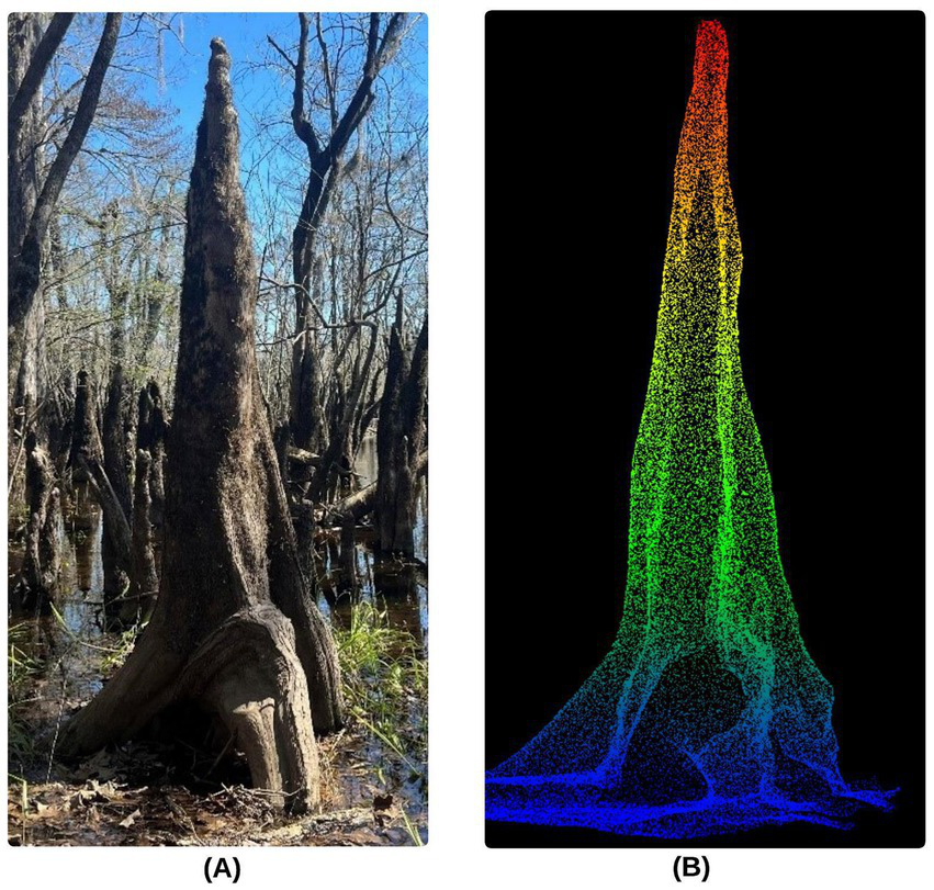
Figure 3
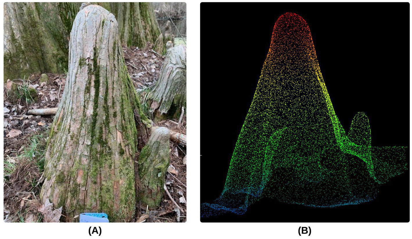
Example of a single knee as seen from a (A) photograph and (B) the point cloud data.
2.3 Data processing
We used four steps to obtain a knee volume estimate from the LiDAR data (Figure 4). First, the LiDAR data went through a pre-processing stage (Step 1), which included registering the scanned data so that a final point cloud could be exported for processing. We then processed the LiDAR point cloud (Step 2) to transform z-values to represent accurate elevation and to classify points as either ground or above ground. The aboveground points were then segmented (Step 3) into objects representing cypress knees. For each object, we used the C-hbS algorithm and CSH method to estimate each object’s volume (Step 4). We compared the volume estimates from the C-hbS and CSH methods to estimates from allometric equations.
Figure 4
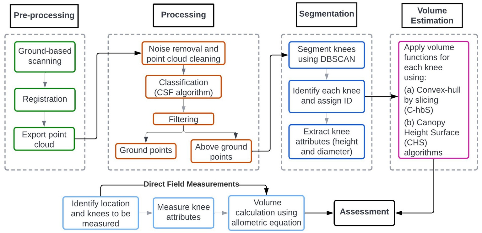
Workflow diagram of the analysis.
Step 1. After the LiDAR data was collected in the field, the point cloud was registered to the three ground control points using the WGS84 Universal Transverse Mercator (UTM) Zone 17 N coordinate system with units in m using the align function within CloudCompare v2.13.alpha, (2023). To ensure that all negative z-values were converted to non-negative values, the x, y, and z values were rotated and translated. The registration had an average accuracy (RMS – Root Mean Square in CloudCompare) of 5–20 cm.
Step 2. The point cloud was further classified using the Cloth Simulation Filter (CSF, Zhang et al., 2016) algorithm in R (RStudio Team, 2019), while all other processes related to volume estimation were implemented in Python using Jupyter Notebook (Kluyver et al., 2016). CSF algorithm simulates a piece of cloth draped over an inverted point cloud. This method turns the point cloud upside down to derive a smoothed, inverted surface. The default parameter values for this algorithm initially classified points as ground points when they were not. Additional parameters were explored with the following values providing the most accurate results: a classification threshold of 0.05, a max iteration value of 500 s, and a cloth resolution value of 0.01 m.
Step 3. We filtered the classified knee points to remove all ground points, outliers, and non-knee points. Filtering the ground points helps isolate the individual knees in the point cloud, facilitating individual knee clustering and segmentation. The Density-Based Spatial Clustering of Applications with Noise (DBSCAN) algorithm is a machine learning algorithm for grouping the data points close to each other in a high-dimensional space (Ester et al., 1996). For each point within a cluster, a neighborhood radius, or maximum distance, is identified such that it contains a minimum number of points (Ahmed and Razak, 2016). We used the DBSCAN algorithm to segment individual knees in the filtered points. DBSCAN was selected as it does not require predetermined cluster counts to cluster datasets with arbitrary shapes and find outliers and noise, making it more flexible than algorithms like k-means (Chen et al., 2011). The scikit-learn library in Jupiter Notebook (Pedregosa et al., 2011) helps automate the volume estimation process.
Step 4. We estimated the volume of the individually segmented knees using the C-hbS and CSH algorithms. A convex hull is a concept in computational geometry that refers to a convex polygon that encloses a given set of points in a geometric space. At the same time, a slice-based convex-hull algorithm involves partitioning the 3D point clouds into horizontal slices and computing the convex hull of each slice individually (Li et al., 2009; Kyriazis et al., 2007). This technique was employed to estimate the volume of each knee by slicing knee objects along the vertical axis into sections, or slices, at a uniform interval of equal thickness (0.02 m) and projecting each slice onto a horizontal plane to compute the convex hull Equation 4. Once the convex hull has been built, its vertices are arranged counterclockwise to ensure consistent orientation. A section curve function was developed for each slice area boundary in a two-dimensional plane.
Given the vertex coordinates , the formula for calculating the convex hull area is:
Where Si in cm2 is the area of the i-th point cloud slice calculated based on the convex hull algorithm are the coordinates in cm of the i-th vertex of the convex hull formed by the knee point cloud slice, and n is the number of vertices.
We then calculated the volume of each slice Equation 5 based on the uniform slice thickness of as follows:
Where is the volume of the i-th slice of the interval, and are the areas in cm2 of the lower and upper borders of the section-volume and is the slice thickness at the i-th layer.
A bias may arise within the convex hull (without slicing) when dealing with concave-shaped objects, causing the convex hull to deviate from closely aligned with the object’s boundaries. We corrected this by slicing the knees to ensure that the thickness of each slice and the number of slice layers were well-adapted to the shape and size of the object. This method does not consider irregularities or inward curvatures in slices or sections, which can lead to overestimation. We then calculated the total volume as the sum of the individual slice volumes between interval lines a-b:
Where is the total volume of the k-th knee in cm3Equation 6.
The other volume estimation method we explored in this study is the CSH method (Fallah and Onur, 2011; Schulze- Brüninghoff et al., 2019), which directly estimates the volume of each knee by partitioning the 3D space into small square grid cells, computing the volume for each grid cell, and summing the contributions across all grid cells within the CSH. We derived the volume by converting points for each knee to a surface using a nearest neighbor interpolation. The accuracy of the interpolation to generate the 3D reconstructed CSH depends on the density of the point cloud and its ability to create stepped or blocky surfaces (Fallah and Onur, 2011). Exploring different resolutions ranging from 0.005 m to 0.05 m, we examined the accuracy of the CSH method in estimating the knees’ volume (Schulze- Brüninghoff et al., 2019).
2.4 Knee density, biomass, and carbon estimation
To obtain an estimate for total biomass, we calculated the biomass of each knee as a function of the specific gravity (wood density) and the volume. To determine the number of knees per hectare, we randomly overlayed a series of 2-meter fixed-radius plots across the study area and counted the number of knees identified from the LiDAR per plot. We multiplied the mean knee biomass by the mean knee density to estimate biomass (Mg) and carbon (Mg C) on a per-hectare basis. Carbon was assumed to be 53.1% of the wood biomass (Middleton, 2020; Woodall et al., 2011).
2.5 Model assessment
Although the C-hbS and CSH algorithms have been used for tree volume estimation (e.g., Hosoi et al., 2013; Li et al., 2009; Yan et al., 2019), the accuracy of their estimates for knee volume has not been studied. To evaluate the accuracy of the LiDAR height estimates, we compared the calculated height from the field measurements to the estimate from the LiDAR point cloud data. We created a scatterplot of the allometric volume estimates versus the LiDAR estimates to visualize the differences and assess measurement error. Additionally, the volume difference estimates, which compared the field volume to the LiDAR estimates (C-hbS and CSH methods), were calculated using 30-centimeter height and 20-centimeter diameter classes. These 30 cm height and 20 cm diameter thresholds were chosen as practical considerations to help segment the knees effectively, allowing for a more precise analysis of distribution patterns and distinctions between smaller and larger knees.
3 Results
3.1 Findings from postprocessing
Figure 5 highlights the comparison of different default parameters for classifying ground points. When the default values proposed by Zhang et al. (2016) were used (Figure 5A), more than half the points were classified as ground points for this specific knee. Point cloud density, topography, and the distribution of non-ground points are some factors that influence the ground-filtering performance. Adjusting the class resolution from 0.5 to 0.05 m and the cloth resolution from 0.5 m to 0.05 m produced a more accurate ground point classification (Figure 5B). Additionally, Figures 5C,D provide a visual example of the segmentation process using the DBSCAN algorithm to identify individual knees. Modifying the parameters for the DBSCAN algorithm influences the number of individual knees that were identified. When we modified the parameters for the DBSCAN algorithm to a maximum distance of 0.05 m, only four individual knees were identified (Figure 5C), while reducing the maximum distance to 0.015 m allows for all five knees to be identified (Figure 5D). As Ester et al. (1996) reported, using global values for maximum distance and minimum points may merge two clusters of different densities that are close to each other.
Figure 5
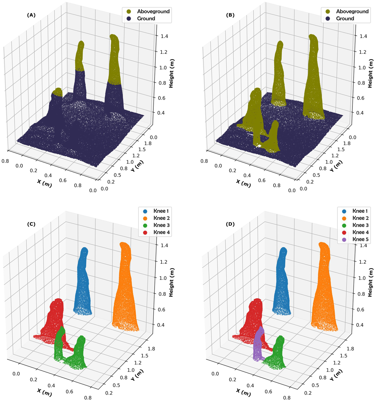
(A) The extracted classified single knee points using the default parameters of the CSF algorithm and, (B) the adjusted parameters in the CSF algorithm, (C) segmented individual knees based on a 0.05-meter maximum distance, and (D) segmented individual knees based on a 0.015-meter maximum distance.
3.2 Volume estimation
When implementing the C-hbS algorithm, we explored different slicing heights and computed their convex hull. Slicing heights from 0.02 to 0.4 m were explored based on the range of height values found from the field estimates (Figures 6C–F). This ensures that the number of slice layers is well adapted to the shape and size of the actual knees (Yan et al., 2019). We overlaid a conical geometry on the point cloud to enhance the visualization and understand the relationship between the field measurements and the point cloud, as depicted in Figure 6A. The convex-hull-without-slicing does not align with the shape of the geometry, leading to an overestimation of volume, as seen in Figure 6B. The results further indicate that a high number of slices per knee (i.e., small slicing height) provides volume estimates that capture the 3D geometric shape in finer detail, allowing for the identification of slight variations in the shape of the objects (Figures 6C–F). Others have found that slicing the convex hull into multiple sections improves the accuracy of the volume calculation compared to a single calculation of the convex hull without slicing (Yan et al., 2019; Zhi et al., 2016).
Figure 6
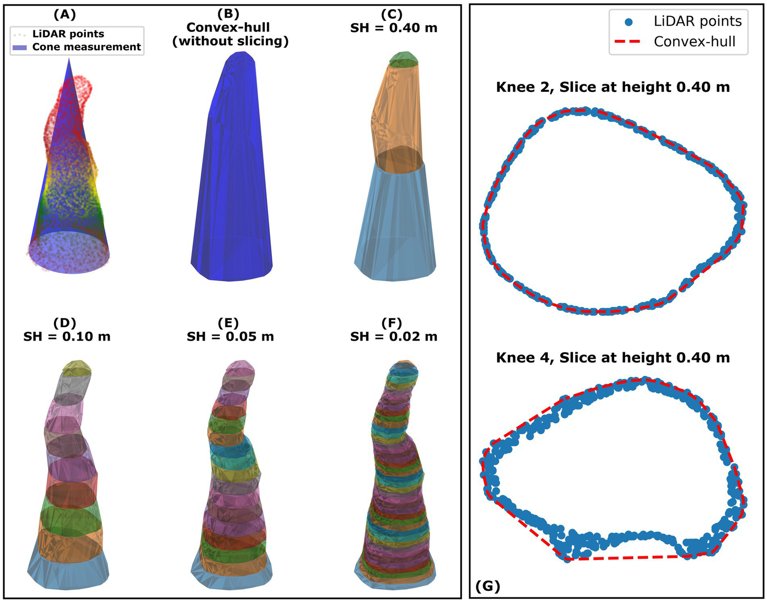
Example of the slicing algorithm applied to an individual knee where (A) illustrates the point cloud as compared to a cone derived from the field measurements, and (B–F) Illustrates differences found from varying slicing heights (m) and (G) shows the cross-section of knee 2 and knee 4 slices at height 0.40 m elevation from the knee base.
For a regular conical-shaped structure, the slicing method surrounds the points without exaggeration because the outline is curved to the exterior of a circle or sphere (i.e., convex). Figure 6G provides a visual for this scenario where the red broken line represents the convex hull. While the number of points and slice shape change along the gradient of a knee, the figure shows the circumferences of the slice containing each point at 0.4 m for two different knees. For the knee with a concave shape (Figure 6G, knee 4), the slicing method does not capture the inward irregularities and tends to simplify the shape slightly. Knee 4, on the other hand, in Figure 6G, has both concavities and cavities on its surface, which leads to overestimation in some sections and a subsequent overestimation of total volume. The convex line (represented in red) does not capture the complexity of the cavities within the irregular shape. The level of overestimation is dependent upon the degree of concavity. In this example, the level of concavity decreases the higher up the knee.
Figure 7 represents an example of applying the CSH algorithm for a single knee, where 0.05 m, 0.01 m, and 0.005 m resolutions were used to compute the volume. Figure 7A provides a comparison of the point cloud to a cone created from the field measurements. In relation to the allometric volume estimates, the volume from the 0.005 m resolution is slightly lower (0.05604 m3, Figure 7A) compared to the one obtained from the 0.01 m (0.05613 m3, Figure 7B) and 0.05 m (0.05690 m3, Figure 7C) resolutions. The volume using the three resolutions was larger compared to the allometric method. Although the difference in volume estimates across all three resolutions is not significant, the finer resolution provides more detail and has the potential to capture the shapes and estimate volume accurately; hence, we selected the 0.005 m resolution for the volume estimation process.
Figure 7
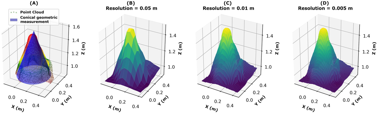
Example of applying the CSH algorithm to an individual knee, where (A) represents the comparison of the point cloud to a cone with dimensions determined from field measurements and (B) through (D) provide visual examples of three different resolutions, (B) 0.05 m, (C) 0.01 m, and (D) 0.005 m.
3.3 Model assessment
The results presented in Figure 8A indicate that the height estimates from the LiDAR point cloud and the field measurements are highly correlated (r = 0.98). However, the LiDAR estimates are slightly higher for the small knees. Factors such as filtering of ground points and slight leaning of knees could influence the LiDAR estimates.
Figure 8
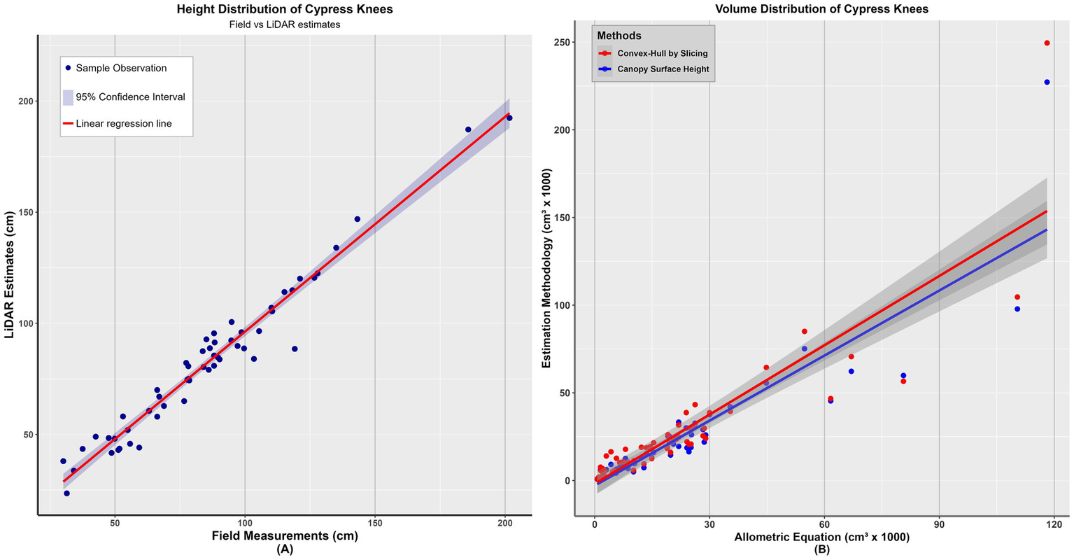
(A) Comparison of height determined from the LiDAR point cloud and the direct field measurements, (B) comparison between the allometric estimate calculated from the field measurements and both the CSH and C-hbS algorithms.
The average volume estimates across the three methods differ, ranging from 22,110 to 27,450 cm3, with a 24% difference between the lowest and highest values (Table 2). The minimum volume for the allometric equation method is 660 cm3, and the maximum estimate is 118,130 cm3, with a standard deviation of 24,820 cm3. The minimum and maximum volume from the C-hbS method are 800 cm3 and 227,200 cm3, respectively, with a standard deviation of 34.19 cm3, while the minimum and maximum volume for the CSH method are 930 m3 and 249.51 cm3, respectively. Additionally, the total volume of all samples using the C-hbS method is 1,335,710 cm3, 9.8% higher than the allometric total volume estimates. In contrast, the CSH method is 21% higher than the allometric estimates.
Table 2
| Method | Minimum | Mean | Maximum | Standard deviation | Total |
|---|---|---|---|---|---|
| Allometric equation | 660 | 22,110 | 118,130 | 24,820 | 1,216,290 |
| Convex-hull by slicing | 800 | 24,290 | 227,200 | 34,190 | 1,335,710 |
| Canopy-surface height | 930 | 27,450 | 249,510 | 37,310 | 1,482,750 |
Summary statistics for individual knee volume based on each method.
All measurements listed are in cm.
The volume estimates using allometric equations are highly correlated to the C-hbS (r = 0.90) and the CSH methods (r = 0.88). Figure 8B indicates that the CSH method has higher estimates for very small knees and lower estimates for large knees than the allometric method, with the largest knee exception. While we see the same pattern between the C-hbS and the allometric method, the discrepancies for the smaller knees were not as substantial. For both algorithmic methods (C-hbS and CSH), the volume differences, when compared to the allometric method, become greater as the knee size increases.
The biggest knee has the largest difference between the C-hbS and CSH methods compared to the allometric method. This knee is the tallest and contains the largest base buttress (Figure 9). The volume estimate for this knee is much greater for the CSH method than the C-hbS method. We calculated the volume for this knee to be 227,207 cm3 using the C-hbS method and 249,510 cm3 for the CSH method, or a 92 and 111% increase in volume, respectively, compared to the allometric estimate of 118,130 cm3.
Figure 9
The largest knee is represented as (A) an image and (B) the corresponding point cloud.
We estimated the bias for model comparison as the difference between the allometric estimate and those from the C-hbS and CSH methods for four specific height classes. The CSH method has a lower median value than the C-hbS method, regardless of height class. The C-hbS method shows an increase in differences as the height class increases (Figure 10A), with most knees exceeding 95 centimeters (cm) generating larger volume estimates compared to the allometric method, while knees <65 cm in height produced slightly similar estimates as the allometric method. The spread in the data also increases for both methods as the height class increases, with a more extensive spread seen for the CSH method. The two data points that stand out represent the tallest knee and a knee with a large base buttress with a narrow stem to the tip after the basal swell.
Figure 10
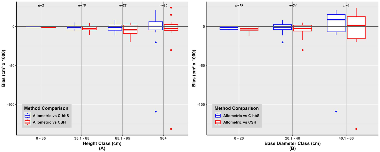
Boxplots of bias values for both the C-hbS and CSH methods as compared to the allometric method across (A) four height classes and (B) three diameter classes.
We also investigated the bias for four diameter classes (Figure 10B). The CSH method has a lower median value than the C-hbS method, regardless of the diameter class. The CSH and C-hbS methods show an increase in difference as the diameter class increases. The spread of the data is largest for the largest diameter class, with the data points that are very different, representing the largest knees and another knee with a large base buttress and a small auxiliary (see Figure 3).
The average wood density of the bald cypress knees is 0.32 g/cm3, with a standard error of 0.02. Stiller (2009) found similar ranges for the wood density of bald cypress, 0.31 g/cm3 – 0.34 g/cm3. Based on the wood density, the estimated total biomass of all sampled knees using the C-hbS is 416,769 g with an average biomass of 7577.25 ± 2,858 g. The results indicate a 10.5% difference in total biomass estimates using the C-hbS algorithm and a 21.9% difference using the CSH algorithm when compared to the allometric estimates. The mean knee biomass is 61.94 ± 23.4 Mg ha–1, while the average knee carbon stock is 32.83 ± 12.38 Mg C ha−1.
4 Discussion
Our results show that LiDAR is a cost-effective and reliable method to capture detailed information on the shape and volume of bald cypress knees. Postprocessing the data allows for distinguishing between ground and non-ground points and creating models and measurements of intricate 3D geometric features. This is achievable based on the distribution of points in the vertical direction (Zhao et al., 2018). It is crucial to select the right resolution during ground classification based on the average distance or spacing between points in the point cloud dataset and including user-defined parameter values (Yilmaz and Karakus, 2013). The DBSCAN algorithm used in the analysis is a density-based clustering algorithm that identifies clusters of arbitrary shape, size, and varying densities. The terrain within the study site is slightly uneven, containing protruding surfaces such as hummock, leaf piles, and other soil protrusions in relation to the knees.
In some cases, DBSCAN identified these protruding surfaces as knee clusters during the clustering analysis, considering that the knees are closer to the ground compared to the tree. To resolve this, we had to remove the non-knee points manually. The classified point cloud needed to be further segmented into individual knee clusters when knees were found next to each other. This individual clustering was necessary to ensure volume estimates were available for individual knees and to automate the volume estimation process.
Disparities in height measurements using the Pythagoras theorem are due to some knee shapes not satisfying the Pythagoras theorem rules well enough (Morin, 2021). For some knees, the slant height was not a straight line from the tip to the ground, as the knees contained irregularities such as concavities or large buttresses. In some instances, the knee buttresses were stout and left a very narrow stem to the tip after the basal swell. A study by Rogers (2021) described them as woody outgrowths with varying sizes and shapes but majorly are either “vaguely conical-club-shaped” or have multiple blunt growing points (Rogers, 2021). In these scenarios, the Pythagoras theorem method will produce a bias leading to overestimation or underestimation of the height and, subsequently, the volume. Defining the base and the leaning height for the small knees was also challenging. In contrast, the estimated height from the LiDAR point cloud is based on subtracting the lowest vertical value from the highest vertical points, a more accurate method.
Previous studies have estimated the biomass and carbon stock of the bald cypress knees using a simple procedure that relates the knees’ shape to a cone volume and subsequently estimates biomass using conversion factors for wood density and carbon (Middleton, 2020). The usefulness of LiDAR data in estimating forest characteristics has been proven in many studies to estimate tree volume and biomass across different species and regions (Bortolot and Wynne, 2005; Demol et al., 2022; Omasa et al., 2006). However, no studies were found to propose using LiDAR data from the iPad Pro 12.9 to estimate the knee volume of bald cypress. Previous studies have shown the high precision of using this device for tree mapping, such as stem counts with a detection rate of 97.3% and diameter measurements with efficient labor effort compared to the traditional approaches (Gollob et al., 2021; Wang et al., 2021). Relating the time taken to measure each knee in the field (approximately 40 s per individual) to scanning individual knees, the remote sensing method is more efficient. However, considering the processing and post-processing procedures, cleaning the data, and performing the volume computation is more time-consuming. Regardless, the LiDAR captures the changes in the surface along the vertical height and irregularities of the knees. The total number of knees per area can also be estimated from the LiDAR data. It also provides a 3D digital representation of each knee, which can be further studied and used to estimate the volume and biomass of all the knees in the area scanned.
When using LiDAR to estimate knee volume, the C-hbS method produced a precise result for knees that followed each slice’s cone-like shape and convex structures. This is in line with a study by Chang et al. (2017), which shows that slicing produces 0 % error in volume for the cubical geometric object. Taller knees will have more slices compared to short knees. The slicing height also determines the accuracy of this method, as thinner and higher numbers of slices have more ability to partition the change in knee height in relation to the diameter and subsequently address shape irregularities. This method further helps address the issue of overestimation of volume, as the surface area of the knee is a key component of determining the volume within each slice. Visualizing the shapes of each slice aids in understanding its internal structure and gaining insights into variations along the vertical axis. Most importantly, this approach helps identify potential voids or cavities and analyze the volume distribution across different sections. Hence, for knees with geometric irregularities around some slices, this method overestimates their volume as the 3D convex geometry does not align with the boundary and edge points of each slice, which overestimates the volume of slices that included gaps and holes (Fernández-Sarría et al., 2013; Yan et al., 2019). The value of the tallest knee is comparable to that found in Louisiana, 288,856 cm3 (Middleton, 2020).
On the other hand, the CSH method produced slightly higher volume estimates than the allometric and Canopy-Surface Height methods. Comparing this result to that of Schulze- Brüninghoff et al. (2019), the CSH method was reported to be the most accurate method for biomass estimating grassland from 3D point clouds. With the availability of dense data, nearest neighbors, a rapid interpolation method, is preferred for forest areas surfaces (Vazirabad and Karslioglu, 2010), hence it was used also in this study. However, there is a significant variation in knee size and shape irregularities. Therefore, the CSH method needs to be adopted to reconstruct the knee structures, calculate the volume, and effectively capture each knee’s details. Another issue to consider when using the CSH method is that it requires more computational time to perform the calculations depending on the resolution; the higher the resolution, the higher the processing time, with this analysis showing an approximate 3–6% increase in computational time when compared to the convex-hull algorithm.
Generally, allometric estimates are consistently smaller after comparing them with the estimates from the two methods because they are underestimating and oversimplifying the complexity of the shape of the knees. Hence, with a better representation of the knee geometry, it is possible to infer that the volume from the LiDAR using the two algorithms is more accurate.
The knee density ha−1 (8174.78 ha−1) in this study is comparable to the densities obtainable in the Mississippi River Alluvial Valley (7,870 ± 814 ha−1, Brown, 1984) and floodplain forests near Gainesville, Florida (10,100 ha−1, Middleton, 2020). Using the volume estimated from the 2 cm C-hbS method, the aboveground mean biomass of the knees in the Three Sisters Swamp is 61.94 ± 23.4 Mg ha−1. Assuming that carbon is 53.1% of wood biomass, the mean carbon biomass represented by the bald cypress knees in this study was substantial (32.83 ± 12.38 Mg C ha−1). This result is similar to what was obtained in the MRAV for flooded sites (33.7 ± 6.4 Mg C ha−1) and flooded swamps in White River (18.1 ± 3.7 Mg C ha−1), which is much higher than the sites not exposed to floods sites (2.9 ± 0.7 Mg C ha−1).
Lastly, this study indicates that using LiDAR increases biomass and carbon estimates by 1–17% for the C-hbS and 10–28% for the CSH method as compared to the allometric method, which could have significant implications for biomass and carbon accounting. This difference is a result of several factors contributing to the volume estimates ranging from proper capture of the knees’ complete 3D/vertical structure by the LiDAR point cloud and the presence of voids and concavities in some knees. Also, oversimplification of the knee shape due to approximation of the knee shape with a cone using the traditional method does not accurately capture all the nuances and complexities of the knee shape. Additionally, the lack of a very clear definition of ground during field measurements contributes to the underestimation of biomass and carbon.
Future research should explore new, advanced point cloud algorithm methods, such as adaptive voxel-based and concave k-nearest algorithms, which could account for structural irregularities in knees and other tree species to provide optimum and precise options. There is also a need to compare the time needed for sampling individual knees using manual field measurements to estimates from LiDAR data. Lastly, using LiDAR to collect data provides an opportunity to minimize laborious fieldwork, thereby maximizing the number of sampled knees and providing data at finer scales. However, processing the data and model development can be time-consuming and require additional technical skills; therefore, traditional techniques are deemed more feasible for quick estimation when shape considerations are not essential.
5 Conclusion
Allometric equations for estimating bald cypress knee volume from traditional field measurements are based on the volume of a cone. This approach does not assume the variability in knee shape, can underestimate the volume of knees with large slants, and overestimates the volume of knees with concavities. We found that volume estimates from allometric equations and traditional field methods were smaller compared to those obtained from algorithm methods applied to the iPhone-derived point cloud. This was due to the ability of the LiDAR point cloud to capture the complexity of knee shapes. Our results indicate that modification of the parameters in the DBSCAN algorithm influenced the number of individual knee segmentations determined from the LiDAR point cloud. Increasing the number of segmentations can allow for greater volume estimation accuracy, especially for small, very close to each other, and steep-leaning objects.
We evaluated the volume estimation of bald cypress knees from the point clouds obtained using iPhone LiDAR technology for bald cypress knees. The high correlation (r = 0.98) between height estimates derived from the LiDAR point cloud and direct field measurements indicates that this technology is a valid alternative to traditional field measurements. In areas where direct field measurements from measuring tapes are difficult, such as areas where the water level is high or it is dangerous to stand in water, using a device such as an iPhone can be a great advantage. While a laser rangefinder provides another alternative to direct field measurements using tape, LiDAR point clouds provide detailed information about the shape of an object, leading to more accurate estimates of volume. When choosing between these options, data processing time and computing needs should be considered.
Our study further highlights the importance of bald cypress knees in contributing to biomass and carbon estimates for these old-growth sites. The estimated knee density (8,174 knees per hectare), aboveground biomass (62 ± 23 Mg per hectare), and carbon (32.83 ± 12.38 Mg C per hectare) in this study site are significant, demonstrating that cypress knees are vital in the teal carbon balance of wetlands in North Carolina. Overall, this study demonstrates a cost-effective remote sensing method for sampling complex conical structures such as bald cypress knees, which can be replicated in other locations. It also provides an alternative to assessing more accurate estimates of volume needed to inform carbon accounting.
Statements
Data availability statement
The original contributions presented in the study are publicly available. This data can be found at: https://github.com/Titilayor547/Knee_Data.
Author contributions
TT: Conceptualization, Data curation, Formal analysis, Methodology, Visualization, Writing – original draft, Writing – review & editing, Investigation. LR: Conceptualization, Funding acquisition, Resources, Supervision, Validation, Visualization, Writing – original draft, Writing – review & editing, Investigation. MA: Data curation, Investigation, Supervision, Writing – original draft, Writing – review & editing, Methodology, Resources. HM: Supervision, Validation, Visualization, Writing – original draft, Writing – review & editing.
Funding
The author(s) declare that financial support was received for the research and/or publication of this article. This work was supported by the Summerville Family Forest Research Award 2021 and the Department of Forestry and Environmental Resources, College of Natural Resources, North Carolina State University.
Acknowledgments
We deeply acknowledge the opportunity and accessibility provided by the Nature Conservancy, the organization managing the research site. A sincere gratitude goes to Dr. David Stahle, whose work serves as a foundation and source of inspiration for this study, and his student Dr. Curtis Hall, who provided the initial videos and images that guided the field trips and shaped the trajectory of this research. Thanks to Dr. Forrester for laboratory assistance and Ivan Raigosa-Garcia and Bini Dahal for their help during the field data collection.
Conflict of interest
The authors declare that the research was conducted in the absence of any commercial or financial relationships that could be construed as a potential conflict of interest.
Correction note
This article has been corrected with minor changes. These changes do not impact the scientific content of the article.
Publisher’s note
All claims expressed in this article are solely those of the authors and do not necessarily represent those of their affiliated organizations, or those of the publisher, the editors and the reviewers. Any product that may be evaluated in this article, or claim that may be made by its manufacturer, is not guaranteed or endorsed by the publisher.
References
1
Ahmed K. N. Razak T. A. (2016). An overview of various improvements of DBSCAN algorithm in clustering spatial databases. Int. J. Adv. Res. Comput. Commun. Eng.5, 360–363.
2
Bortolot Z. J. Wynne R. H. (2005). Estimating forest biomass using small footprint LiDAR data: an individual tree-based approach that incorporates training data. ISPRS J. Photogramm. Remote Sens.59, 342–360. doi: 10.1016/j.isprsjprs.2005.07.001
3
Briand C. H. (2021). Cypress knees: an enduring enigma. Arnodia60, 19–25.
4
Bridgham S. D. Megonigal J. P. Keller J. K. Bliss N. B. Trettin C. (2006). The carbon balance of north American wetlands. Wetlands26, 889–916. doi: 10.1672/0277-5212(2006)26[889:TCBONA]2.0.CO;2
5
Brown C. A. (1984). “Morphology and biology of cypress trees” in Cypress swamps. eds. EwelK. C.OdumH. T. (Gainesville, FL: University Presses of Florida).
6
Bureau of Outdoor Recreation (1971). The Black River: North Carolina and South Carolina. Available online at: http://npshistory.com/publications/nwsr/nc-black.pdf#:~:text=The%20soils%20along%20the%20stream%20are%20sandy-loam%2C%20thua,flood%20plain%20is%20covered%20with%20bottom%27%20land%20hardwoods (Accessed August 3, 2022).
7
Cao L. Coops N. C. Innes J. L. Sheppard S. R. J. Fu L. Ruan H. et al . (2016). Estimation of forest biomass dynamics in subtropical forests using multi-temporal airborne LiDAR data. Remote Sens. Environ.178, 158–171. doi: 10.1016/j.rse.2016.03.012
8
Chang W.-C. Wu C.-H. Tsai Y.-H. Chiu W.-Y. (2017). Object volume estimation based on 3D point cloud. 2017 CACS22, 1–5. doi: 10.1109/CACS.2017.8284244
9
Chen X. Liu W. Qiu H. Lai J. (2011). Apscan: a parameter-free algorithm for clustering. Pattern Recogn. Lett.32, 973–986. doi: 10.1016/j.patrec.2011.02.001
10
CloudCompare v2.13.alpha . (2023). Computer software. Available online at: http://www.cloudcompare.org/ (Accessed June 13, 2023).
11
Davidson E. A. Janssens I. A. (2006). Temperature sensitivity of soil carbon decomposition and feedbacks to climate change. Nature440, 165–173. doi: 10.1038/nature04514
12
Demol M. Verbeeck H. Gielen B. Armston J. Burt A. Disney M. et al . (2022). Estimating forest aboveground biomass with terrestrial laser scanning: current status and future directions. Methods Ecol. Evol.13, 1628–1639. doi: 10.1111/2041-210X.13906
13
Dong L. Zhang L. Li F. (2014). A compatible system of biomass equations for three conifer species in Northeast China. For. Ecol. Manag.329, 306–317. doi: 10.1016/j.foreco.2014.05.050
14
Ester M. Kriegel H. P. Sander J. Xu X. (1996). A density-based algorithm for discovering clusters in large spatial databases with noise. Knowledge Discovery Data Mining96, 226–231.
15
Fallah Y. Onur M. (2011). “Lidar for biomass estimation” in Biomass—Detection, production and usage. ed. MatovicM. D. (London: InTech).
16
Fernández-Sarría A. Velázquez-Martí B. Sajdak M. Martínez L. Estornell J. (2013). Residual biomass calculation from individual tree architecture using a terrestrial laser scanner and ground-level measurements. Comput. Electron. Agric.93, 90–97. doi: 10.1016/j.compag.2013.01.012
17
Gollob C. Ritter T. Kraßnitzer R. Tockner A. Nothdurft A. (2021). Measurement of Forest inventory parameters with apple iPad pro and integrated LiDAR technology. Remote Sens.13:3129. doi: 10.3390/rs13163129
18
Gonzalez P. Asner G. P. Battles J. J. Lefsky M. A. Waring K. M. Palace M. (2010). Forest carbon densities and uncertainties from lidar, QuickBird, and field measurements in California. Remote Sens. Environ.114, 1561–1575. doi: 10.1016/j.rse.2010.02.011
19
Hermosilla T. Ruiz L. A. Kazakova A. N. Coops N. C. Moskal L. M. (2014). Estimation of forest structure and canopy fuel parameters from small-footprint full-waveform LiDAR data. Int. J. Wildland Fire23:224. doi: 10.1071/WF13086
20
Horan J. (2020). River of time: The stunning old-growth forest in the three sisters swamp. NC State University: Raleigh, NC.
21
Hosoi F. Nakai Y. Omasa K. (2013). 3-D voxel-based solid modeling of a broad-leaved tree for accurate volume estimation using portable scanning lidar. ISPRS J. Photogramm. Remote Sens.82, 41–48. doi: 10.1016/j.isprsjprs.2013.04.011
22
Hossain M. Siddique M. R. H. Saha S. Abdullah S. M. R. (2015). Allometric models for biomass, nutrients and carbon stock in Excoecaria agallocha of the Sundarbans, Bangladesh. Wetl. Ecol. Manag.23, 765–774. doi: 10.1007/s11273-015-9419-1
23
Hudak A. T. Strand E. K. Vierling L. A. Byrne J. C. Eitel J. U. H. Martinuzzi S. et al . (2012). Quantifying aboveground forest carbon pools and fluxes from repeat LiDAR surveys. Remote Sens. Environ.123, 25–40. doi: 10.1016/j.rse.2012.02.023
24
Janzen D. H. (1974). Tropical Blackwater rivers, animals, and mast fruiting by the Dipterocarpaceae. Biotropica6:69. doi: 10.2307/2989823
25
Kato A. Moskal L. M. Schiess P. Swanson M. E. Calhoun D. Stuetzle W. (2009). Capturing tree crown formation through implicit surface reconstruction using airborne lidar data. Remote Sens. Environ.113, 1148–1162. doi: 10.1016/j.rse.2009.02.010
26
Ketterings Q. M. Coe R. van Noordwijk M. Ambagau’ Y. Palm C. A. (2001). Reducing uncertainty in the use of allometric biomass equations for predicting aboveground tree biomass in mixed secondary forests. For. Ecol. Manag.146, 199–209. doi: 10.1016/S0378-1127(00)00460-6
27
Kluyver T. Ragan-Kelley B. Fernando P. Granger B. Bussonnier M. Frederic J. et al . (2016). “Jupyter Notebooks – a publishing format for reproducible computational workflows,” in Positioning and Power in Academic Publishing: Players, Agents and Agendas. eds. LoizidesF.SchmidtB.. 87–90.
28
Korhonen L. Vauhkonen J. Virolainen A. Hovi A. Korpela I. (2013). Estimation of tree crown volume from airborne lidar data using computational geometry. Int. J. Remote Sens.34, 7236–7248. doi: 10.1080/01431161.2013.817715
29
Kyriazis I. Fudos I. Palios L. (2007). “Detecting features from sliced point clouds,” in Proceedings of the Second International Conference on Computer Graphics Theory and Applications, GM/R.
30
Lamborn R. H. (1890). The knees of the bald cypress: a new theory of their function. Science15, 65–67. doi: 10.1126/science.ns-15.365.65
31
Li M. Lu Z. Huang L. (2009). “An approach to 3D shape blending using point cloud slicing,” in 2009 IEEE 10th International Conference on Computer-Aided Industrial Design & Conceptual Design, 919–922.
32
Library of Congress (2015). Lack River (Sampson County-Pender County, N.C.) [government]. Washington, DC: Library of Congress.
33
Lu J. Wang H. Qin S. Cao L. Pu R. Li G. et al . (2020). Estimation of aboveground biomass of Robinia pseudoacacia forest in the Yellow River Delta based on UAV and backpack LiDAR point clouds. Int. J. Appl. Earth Obs. Geoinf.86:102014. doi: 10.1016/j.jag.2019.102014
34
Luetzenburg G. Kroon A. Bjørk A. A. (2021). Evaluation of the apple iPhone 12 pro LiDAR for an application in geosciences. Sci. Rep.11:22221. doi: 10.1038/s41598-021-01763-9
35
Meyer E. (2020). Taxodium distichum. Raleigh, NC: North Carolina State University.
36
Middleton B. (2020). Carbon stock trends of baldcypress knees along climate gradients of the Mississippi River Alluvial Valley using allometric methods. For. Ecol. Manag.461:117969. doi: 10.1016/j.foreco.2020.117969
37
Mokroš M. Mikita T. Singh A. Tomaštík J. Chudá J. Wężyk P. et al . (2021). Novel low-cost mobile mapping systems for forest inventories as terrestrial laser scanning alternatives. Intern. J. Appl. Earth Observa. Geoinfor.104:102512. doi: 10.1016/j.jag.2021.102512
38
Morin D. (2021). “Pythagorean theorem” in Algebra & Geometry for the Enthusiastc beginner. ed. MusiliC. (Cham: Springer), 255–312.
39
Nahlik A. M. Fennessy M. S. (2016). Carbon storage in U.S.Nat. Commun.7:13835.
40
North Carolina Division of Parks and Recreation (NCDPR) . Feasibility study of establishing a state park along the Black River in Sampson, Bladen and Pender counties. (2018). Available at: https://webservices.ncleg.gov/ViewDocSiteFile/28207 (Accessed June 11, 2025).
41
Omasa K. Hosoi F. Konishi A. (2006). 3D lidar imaging for detecting and understanding plant responses and canopy structure. J. Exp. Bot.58, 881–898. doi: 10.1093/jxb/erl142
42
Parresol B. R. (2002). Baldcypress, an important wetland tree species: Ecological value, management and mensuration. In: Nanjing international wetlands symposium, wetland restoration and management: Addressing Asian issues through international collaboration, Nanjing, China. 8–18.
43
Pedregosa F. Varoquaux G. Gramfort A. Michel V. Thirion B. Grisel O. et al . (2011). Scikit-learn: machine learning in Python. J. Mach. Learn. Res.12, 2825–2830.
44
Polycam (2023). Polycam-LiDAR 3D scanner (version 3.1.3) [computer software]. San Francisco, CA: Polycam.
45
Rogers G. K. (2021). Bald cypress knees, Taxodium distichum (Cupressaceae): an anatomical study, with functional implications. Flora278:151788. doi: 10.1016/j.flora.2021.151788
46
RStudio Team (2019). RStudio: Integrated development for R. (version 4.2.1) [computer software]. Boston, MA: RStudio, Inc.
47
Sagang L. B. T. Momo S. T. Libalah M. B. Rossi V. Fonton N. Mofack G. I. et al . (2018). Using volume-weighted average wood specific gravity of trees reduces bias in aboveground biomass predictions from forest volume data. For. Ecol. Manag.424, 519–528. doi: 10.1016/j.foreco.2018.04.054
48
Schulze- Brüninghoff D. Hensgen F. Wachendorf M. Astor T. (2019). Methods for LiDAR-based estimation of extensive grassland biomass. Comput. Electron. Agric.156, 693–699. doi: 10.1016/j.compag.2018.11.041
49
Shi L. Liu S. (2017). “Methods of estimating Forest biomass: a review” in Biomass volume estimation and valorization for energy. ed. TumuluruJ. S. (London: InTech).
50
Stahle D. W. Burnette D. J. Villanueva J. Cerano J. Fye F. K. Griffin R. D. et al . (2012). Tree-ring analysis of ancient baldcypress trees and subfossil wood. Quat. Sci. Rev.34, 1–15. doi: 10.1016/j.quascirev.2011.11.005
51
Stahle D. W. Cleaveland M. K. Hehr J. G. (1988). North Carolina climate changes reconstructed from tree rings: a.D. 372 to 1985. Science240, 1517–1519. doi: 10.1126/science.240.4858.1517
52
Stahle D. W. Edmondson J. R. Howard I. M. Robbins C. R. Griffin R. D. Carl A. et al . (2019). Longevity, climate sensitivity, and conservation status of wetland trees at Black River, North Carolina. Environ. Res. Commun.1:041002. doi: 10.1088/2515-7620/ab0c4a
53
Stiller V. (2009). Soil salinity and drought alter wood density and vulnerability to xylem cavitation of baldcypress (Taxodium distichum (L.) rich.) seedlings. Environ. Exp. Bot.67, 164–171. doi: 10.1016/j.envexpbot.2009.03.012
54
Swetnam T. L. Gillan J. K. Sankey T. T. McClaran M. P. Nichols M. H. Heilman P. et al . (2018). Considerations for achieving cross-platform point cloud data fusion across different dryland ecosystem structural states. Front. Plant Sci.8:2144. doi: 10.3389/fpls.2017.02144
55
Taylor K. (2005). The scenic Black River. AVailable online at: http://scenicnc.com/black_river.html (Accessed February 25, 2023).
56
van Leeuwen M. Nieuwenhuis M. (2010). Retrieval of forest structural parameters using LiDAR remote sensing. Eur. J. Forest Res.129, 749–770. doi: 10.1007/s10342-010-0381-4
57
Vashum K. Jayakumar S. (2012). Methods to estimate aboveground biomass and carbon stock in natural forests—a review. J. Ecosystem Ecogr.2:1000116. doi: 10.4172/2157-7625.1000116
58
Vauhkonen J. Seppänen A. Packalén P. Tokola T. (2012). Improving species-specific plot volume estimates based on airborne laser scanning and image data using alpha shape metrics and balanced field data. Remote Sens. Environ.124, 534–541. doi: 10.1016/j.rse.2012.06.002
59
Vazirabad Y. F. Karslioglu M. O. (2010). “Airborne laser scanning data for single tree characteristics detection,” in Istanbul Workshop, Modelling of Optical Airborne and Space Borne Sensors, XXXVIII.
60
Wang X. Singh A. Pervysheva Y. Lamatungga K. E. Murtinová V. Mukarram M. et al . (2021). Evaluation of Ipad pro 2020 LiDAR for estimating tree diameters in urban forest. ISPRS Ann. Photogramm. Remote Sens. Spat. Inf. Sci.7, 105–110. doi: 10.5194/isprs-annals-VIII-4-W1-2021-105-2021
61
Wilhite L. P. Toliver J. R. (1990). “Taxodium distichum (L.) Rich., baldcypress” in Silvics of North America. eds. BurnsM.HonkalaH. (Washington, DC: United States Department of Agriculture), 563–572.
62
Woodall C. W. Heath L. S. Domke G. M. Nichols M. C. (2011). Methods and equations for estimating aboveground volume, biomass, and carbon for trees in the U.S. forest inventory, 2010. Washington, DC: United States Department of Agriculture.
63
Yan Z. Liu R. Cheng L. Zhou X. Ruan X. Xiao Y. (2019). A concave hull methodology for calculating the crown volume of individual trees based on vehicle-borne LiDAR data. Remote Sens.11:623. doi: 10.3390/rs11060623
64
Yilmaz O. Karakus F. (2013). “Stereo and Kinect fusion for continuous 3D reconstruction and visual odometry,” in 2013 International Conference on Electronics, Computer and Computation (ICECCO), 115–118.
65
Yoshida J. (2020). Breaking down iPad pro 11's LiDAR scanner. Available online at: https://www.eetimes.com/breaking-down-ipad-pro-11s-lidar-scanner/ (Accessed April 10, 2022).
66
Yusup A. Halik Ü. Keyimu M. Aishan T. Abliz A. Dilixiati B. et al . (2023). Trunk volume estimation of irregular shaped Populus euphratica riparian forest using TLS point cloud data and multivariate prediction models. Forest Ecosystems10:100082. doi: 10.1016/j.fecs.2022.100082
67
Zhang W. Qi J. Wan P. Wang H. Xie D. Wang X. et al . (2016). An easy-to-use airborne LiDAR data filtering method based on cloth simulation. Remote Sens.8:501. doi: 10.3390/rs8060501
68
Zhao K. Suarez J. C. Garcia M. Hu T. Wang C. Londo A. (2018). Utility of multitemporal lidar for forest and carbon monitoring: Tree growth, biomass dynamics, and carbon flux. Remote Sens. Environ.204, 883–897. doi: 10.1016/j.rse.2017.09.007
69
Zhi Y. Zhang Y. Chen H. Yang K. Xia H. (2016). “A method of 3D point cloud volume calculation based on slice method,” in Proceedings of the 2016 International Conference on Intelligent Control and Computer Application. 2016 International Conference on Intelligent Control and Computer Application (ICCA 2016), Zhengzhou, China.
Summary
Keywords
bald cypress, carbon, volume estimation, LiDAR, biomass, forested wetlands, allometric estimate
Citation
Tajudeen TT, Rathbun LC, Ardón M and Mitasova H (2025) Carbon estimation of old-growth bald cypress knees using mobile LiDAR. Front. For. Glob. Change 8:1427376. doi: 10.3389/ffgc.2025.1427376
Received
03 May 2024
Accepted
30 May 2025
Published
18 June 2025
Corrected
19 June 2025
Volume
8 - 2025
Edited by
Marco Andrew Njana, Wildlife Conservation Society, Tanzania
Reviewed by
Weizhen Hou, Harvard University, United States
Fugen Jiang, Central South University Forestry and Technology, China
Updates
Copyright
© 2025 Tajudeen, Rathbun, Ardón and Mitasova.
This is an open-access article distributed under the terms of the Creative Commons Attribution License (CC BY). The use, distribution or reproduction in other forums is permitted, provided the original author(s) and the copyright owner(s) are credited and that the original publication in this journal is cited, in accordance with accepted academic practice. No use, distribution or reproduction is permitted which does not comply with these terms.
*Correspondence: Titilayo T. Tajudeen, tttajude@ncsu.edu
Disclaimer
All claims expressed in this article are solely those of the authors and do not necessarily represent those of their affiliated organizations, or those of the publisher, the editors and the reviewers. Any product that may be evaluated in this article or claim that may be made by its manufacturer is not guaranteed or endorsed by the publisher.