Urban tree planting should consider local characteristics: assessing spatial heterogeneity in canopy cooling effects on land surface temperature using Bayesian spatially varying coefficient models

Introduction: Urban trees are essential for mitigating elevated temperatures in cities worldwide, with many municipalities implementing large-scale urban tree planting initiatives. However, the cooling potential of tree canopy coverage is often estimated as a constant value across study areas, despite evidence that temperature reductions depend on local characteristics, including tree traits and urban geometry.

Methods: We evaluated the ability of Bayesian Spatially Varying Coefficient (SVC) models to capture local variability in the cooling potential of urban trees. The model, implemented in R-INLA, integrated Landsat 8 and 9 Land Surface Temperature (LST) data with aerial LiDAR data. Model performance was assessed using validation metrics obtained through 10-fold spatial cross-validation.

Results: Although the SVC did not outperform simpler spatio-temporal approaches according to validation metrics, the spatial distribution of local canopy cooling capacity revealed substantial spatial variability. Average estimated values of canopy cooling capacity on LST (defined as the change in LST associated with a 10% increase in tree canopy cover) were −0.28 °C in vacant lands and −0.09 °C in wooded areas.

Discussion: By providing local estimates, our model underscores how the cooling capacity of tree canopy in built-up environments varies substantially across space. This finding demonstrates the importance of accounting for local environmental characteristics in urban planning and serves as an example of a modeling approach that integrates both local-scale variability in canopy cooling capacity and spatial extent. These results encourage policymakers to adopt context-specific strategies for urban tree planting initiatives rather than applying uniform approaches.

1 Introduction

Currently, 57.7% of the global population lives in urban areas, a proportion expected to rise to 67.9% by 2050 (UN, 2025). This rapid urban expansion is profoundly transforming land use systems, with consequences for biodiversity and environmental sustainability (Houghton et al., 2012; Seto et al., 2012; Phelan et al., 2015). Among its most pressing impacts is the growing threat posed by extreme temperatures in urban environments, which have resulted in severe public health crises. The three deadliest extreme heat events of the 21st century alone have caused nearly 200,000 deaths across Europe (Robine et al., 2008; Barriopedro et al., 2011; Ballester et al., 2023). Future projections of urban warming depict an increasingly concerning scenario, exacerbated by the intensification of the Urban Heat Island (UHI) effect (Chapman et al., 2017), the rising frequency, intensity, duration, and spatial extent of heatwaves (Lorenzo et al., 2021; Domeisen et al., 2023), and the synergistic interaction between UHI and extreme heat events (Founda and Santamouris, 2017).

These challenges underscore the urgent need for effective adaptation and mitigation strategies to address the environmental issues faced by cities (UN, 2023). The scientific literature has explored numerous approaches to enhancing urban livability (Yu et al., 2020). Among these, urban tree planting has gained increasing recognition as a nature-based solution for mitigating multiple environmental challenges, primarily due to its capacity to provide essential ecosystem services (Pataki et al., 2021; Schwaab et al., 2021).

The capacity of urban trees to reduce temperatures has been studied using multiple methods and across different spatial scales. However, there is often a trade-off between the fine-scale variability detected in field-based microclimate studies and the broader extensibility afforded by analyses that rely on remote sensing data. In general, the greater the analytical detail, the lower the potential to scale results to larger study areas. Trees improve thermal comfort by providing shade, reducing surface radiation, and increasing air humidity through evapotranspiration (Oke et al., 2017). At the local scale, research suggests that the cooling capacity of urban trees exhibits substantial temporal and spatial variability (Ziter et al., 2019; Hallar et al., 2021; Locke et al., 2024; Ettinger et al., 2024). This variability is influenced both by urban geometry (Tsin et al., 2016; Kelly-Turner et al., 2022; Li et al., 2024; Li et al., 2025) and by tree traits (Rahman et al., 2020; Miedema-Brown and Anand, 2022; Sharmin et al., 2023; Alonzo et al., 2025). In this context, mature and vigorous trees (Endreny, 2018), large-diameter and long-lived trees (Lindenmayer et al., 2012; Lindenmayer and Laurance, 2016), as well as trees with fuller crowns and more extensive leaf surface areas (Gómez-Muñoz et al., 2010) provide greater ecosystem services and consequently enhanced cooling capacity. Functional traits such as specific leaf area, photosynthetic rate, and water-use strategies determine how trees respond to urban stressors including drought, heat, and pollution, ultimately shaping their capacity to provide cooling (Esperón-Rodríguez et al., 2020; Cho et al., 2024; Ramachandran et al., 2024). In parallel to these findings, but without the same level of trait-specific detail, studies employing high-resolution LST data have also demonstrated high variability in urban cooling capacity as a function of the local characteristics of the study unit (Bartesaghi-Koc et al., 2020; Ossola et al., 2021; Xu et al., 2021; Ahmad et al., 2024; Zhou et al., 2025).

A substantial body of literature has focused on estimating the cooling potential of cities associated with increases in urban canopy cover at the city scale. Given the broad spatial extent of these studies, it is not feasible to account for fine-scale variability, leading to the common assumption of homogeneous cooling capacities within cities. The estimated temperature reductions vary considerably depending on multiple factors, including whether LST or two-step process models to estimate air temperature are considered, the extent of canopy expansion, observational scales, estimation models and methods, and local climate conditions (Logan et al., 2020; Krayenhoff et al., 2021; Marando et al., 2022; Iungman et al., 2023; Wang et al., 2024).

City-level estimates provide a broad overview of the benefits of increasing tree canopy coverage but fail to capture localized temperature reduction effects. The capacity of tree canopy expansion to lower temperatures has also been studied at the block or census scale to obtain estimates at a scale more operational for urban planning (Chakraborty et al., 2022; Francis et al., 2023; McDonald et al., 2024). Similarly, this relationship has been analyzed using grid-based observational units (i.e., pixel-support) across multiple spatial scales (Kong et al., 2014; Hou and Estoque, 2020; Yang et al., 2021; Yuan et al., 2021), primarily capturing the cooling effects associated with increases in canopy cover within observational units defined by grid size.

Despite differences in the spatial scale at which estimates of canopy contributions to temperature reduction have been conducted (ranging from the city scale, to neighborhoods or administrative units, or to grid cells) in all cases it is typically assumed that the relationship between canopy cover and temperature is homogeneous across observational units. In other words, it is assumed that local factors do not influence the capacity of the canopy to provide cooling, and that this ecological process operates uniformly across the city. To account for the variability documented in microscale studies of urban tree cooling, several works have considered such heterogeneity as spatial variability in the cooling capacity of urban canopy cover within individual cities, although this perspective has received comparatively limited attention in the literature.

Spatially explicit models that estimate spatially varying coefficients offer a valuable framework for analyzing the heterogeneity, or non-stationarity, of the relationship between canopy cover and LST (Rollinson et al., 2021). Among these, Geographically Weighted Regression (GWR) (Fotheringham et al., 2009) and Generalized Additive Models (GAMs) (Wood, 2017) are commonly used approaches that provide additional flexibility for modeling complex, spatially varying covariate effects. GWR requires the a priori specification of parameters controlling the spatial kernel and bandwidth, which can heavily influence model outcomes and hinder interpretability (Finley, 2011). GAMs can accommodate spatial dependence in covariate effects through linear combinations of basis functions, yet they also necessitate assumptions regarding the number and placement of knots, which may lead to over-smoothed and potentially biased estimates (Stein, 2014). Consequently, intra-city differences in the cooling effects of urban tree canopy cover have been examined almost exclusively, so far as we are aware, using GWR (e.g., Chen and Lin, 2021; Li et al., 2021; Liu et al., 2022; Francis et al., 2023).

Bayesian Spatially Varying Coefficient (SVC) models (Gelfand et al., 2003) offer an attractive alternative, as their hierarchical structure provides great flexibility for modeling complex data. SVC models allow regression coefficients to vary smoothly across space, employing Gaussian Process specifications when working with geostatistical data (Banerjee et al., 2014; Finley and Banerjee, 2020). While Bayesian SVC models are more complex than the aforementioned approaches, they offer several advantages: they enable full uncertainty propagation, eliminate the need for a priori decisions on grid size or parameter values, and have been shown to outperform GWR in various simulation and empirical studies (Wheeler and Calder, 2007; Finley, 2011). Moreover, SVCs provide a more straightforward interpretation of the estimated effect. By allowing the relationship between canopy cover and temperature to vary across space, SVCs acknowledge that each observational unit is subject to specific micro-scale influences and factors, likely reflecting unobserved variables not included in the model that shape the cooling process, and that this variability and influence also depend on the spatial proximity among units. Nevertheless, the flexibility of SVC models can present both computational and practical challenges. In particular, the Bayesian framework’s requirement to quantify uncertainty for every random variable often leads to substantial computational costs (Thorson et al., 2023). State-of-the-art Bayesian methods, such as the Integrated Nested Laplace Approximation (INLA) framework (Rue et al., 2009), significantly simplify their implementation and dramatically reduce computational costs, making them a particularly relevant alternative for SVC model applications (Bachl et al., 2019).

Urban planners require localized estimates of the cooling capacity of urban tree canopy cover, as these align with the scale of urban interventions and planning processes. Additionally, the effects of tree canopy on temperatures in urban environments are unlikely to be spatially uniform due to complex interactions with urban geometry characteristics and the specific tree traits within each observational unit. Consequently, it is necessary to develop methods that incorporate this variability in cooling capacity at the micro-habitat scale. In addition, these methods must allow for full uncertainty propagation to avoid overoptimistic estimations (Gelman et al., 2013) and the potential negative and costly consequences that may result (Mannucci et al., 2023).

In this study, we explore the potential of SVC models as a modeling tool to account for micro-scale variability in the cooling capacity associated with increases in canopy cover, which, to the best of our knowledge, has not been explored yet. This approach allows for the assessment of spatial variability in the cooling capacity of urban tree canopy across the entire urban matrix, which we hypothesize that it models residual variation not accounted by the model due to unobserved covariables that reflect variation in tree traits and the urban geometry characterizing each observational unit. The model leverages Landsat 8–9 LST and aerial LiDAR data, incorporating uncertainty quantification within a Bayesian framework at an operational scale of 900 m².

The Landsat program has provided high-quality, multispectral spatial data at a global scale for over 50 years. This sustained effort has greatly advanced the study of key environmental processes, including climate change, ecosystem monitoring, water resource management, and forest and agricultural planning (Wulder et al., 2022). With regard to the use of data from its thermal infrared sensors, and consequently for LST derived research, Landsat stands out as one of the most widely accepted and utilized data sources, as highlighted in recent reviews on UHIs studies (e.g., Li et al., 2023; Rajagopal et al., 2023; Cheval et al., 2024). Moreover, Landsat-derived LST has been widely employed in studies addressing environmental sustainability and urban greening (e.g., Li et al., 2024; Pande et al., 2024).

LiDAR technology has become a fundamental tool in forestry science, in its various forms including terrestrial laser scanning, aerial LiDAR, and full-waveform LiDAR, for deriving multiple metrics that quantify canopy distribution, structure, and complexity (Koenig and Höfle, 2016; Åkerblom and Kaitaniemi, 2021; Coops et al., 2021; Fassnacht et al., 2023; Balestra et al., 2024). In urban forestry, this technology is increasingly prominent due to its ability to support the development of urban tree inventories and to cover larger areas when aerial LiDAR is employed (Casalegno et al., 2017; Shojanoori and Shafri, 2016; Zięba-Kulawik et al., 2021; Münzinger et al., 2022; Sharma et al., 2025). In this context, LiDAR technology has been extensively applied across various disciplines and fields within urban sciences, establishing itself as a fundamental tool for advancing environmental sustainability (Liu et al., 2019; Kovanič et al., 2023; Xu et al., 2025). In the present study, discrete-return aerial LiDAR serves as an essential tool to derive urban forest canopy cover across the entire urban matrix of the study area.

Our ultimate goal is to provide policymakers and decision-makers with actionable insights for the strategic integration of urban trees into planning processes, taking into account potential spatial differences in cooling effects and associated uncertainties. We aim to support the development of sustainable, resilient, and healthy urban environments while contributing to climate change adaptation efforts.

2 Materials and methods

2.1 Study area

Málaga has a population of 591,637 inhabitants, making it the sixth most populated city in Spain (NIS, 2024). It is a coastal city characterized by warm summers and mild winters, with an average annual temperature of 18.5 °C and an average annual total precipitation of 534 mm (SMA, 2025). The urban matrix of Málaga was selected as the study area (Figure 1). Two datasets were used for this delineation: (1) The Urban Information System (UIS, 2024), which serves as the primary reference for urban planning and land classification in Spain. “Urban land” and “general systems” located within urban areas were considered. (2) SIOSE-AR (NIG, 2017), a local land use database, was used to extract areas classified as “non-built land,” “highways and expressways,” “roads” and “urban streets” within the zones identified in the previous step. This ensured the creation of a continuous and gap-free surface representing the urban matrix. This vector-based information was rasterized and co-registered to a pixel size of 30 × 30 m, matching the Landsat resolution, to ensure full alignment of the study area with the LST grid.

Figure 1

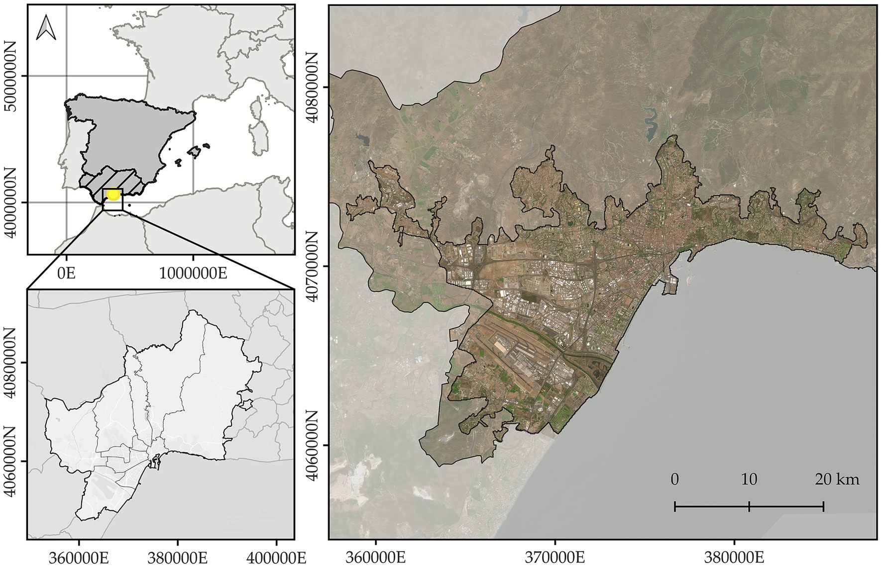
Figure 1. Geographic Location of the Study Area focusing on the urban matrix. The background information includes data from the Spanish National Geographic Institute for the boundaries of Spain and its municipalities. The orthophotography used is from the 2022 National Plan for Aerial Orthophotography project (NIG, 2022). Map represented in coordinate reference system: EPSG 25830.

2.2 Landsat 8 land surface temperature

Landsat 8 and 9 Collection 2 Level 2 Tier 1 data (USGS, 2020) was accessed using Google Earth Engine (Gorelick et al., 2017) via rgee package v.1.1.7 (Aybar et al., 2020). LST is reported in Kelvin on a 30 m grid, consistent with shortwave datasets, despite the raw thermal infrared data having a coarser nominal resolution of 100 m (Crawford et al., 2023). All available images of the study area from 2022 and 2023 (n = 262) were selected for analysis. The Landsat Collection 2 Quality Bands were used to mask pixels affected by cloud cover, cloud shadows, cirrus, radiometric saturation, or atmospheric aerosols in each image. Seasonal means were computed based on the standard meteorological seasons: spring (March 1 – May 31), summer (June 1 – August 31), autumn (September 1 – November 30), and winter (December 1 – February 28/29).

2.3 Description of the covariables

LST for each season was used as the response variable in the modeling process. Each observational unit was defined based on Landsat pixels, represented as grid cells with a spatial resolution of 30 × 30 meters. Higher-resolution covariates were aggregated to match the spatial scale of these observational units. The following datasets were used to generate the model covariates.

1) Cadastral data (CEO, 2024): Spatial information on building footprints was downloaded and processed to calculate the percentage of each observational unit occupied by buildings.

2) SIOSE-AR (NIG, 2017): This dataset was used to generate compositional data at the pixel level due to its scale of 1:1000–1:5,000 m. The percentage of each pixel occupied by vacant land or bare soil was calculated, considering its significant influence on surface UHIs in Mediterranean climates (Unal Cilek and Cilek, 2021). The following land cover classes were reclassified as vacant areas: “non-built land,” “paths and trails,” “meadows,” “grasslands,” “grassland-shrubland,” “shrubland” and “bare or sparsely vegetated land”

3) Variables derived from Second Cover aerial LiDAR data from PNOA (NIG, 2022): The lidR package v. 4.1.2 (Roussel et al., 2020; Roussel and Auty, 2024) was used for point cloud data processing. Canopy height models with a 1 m resolution were developed, applying a minimum height threshold of 3 m and a maximum of 30 m to identify trees and avoid the inclusion of misclassified objects. Canopy cover per pixel was calculated as the area occupied by tree crowns.

LiDAR classes “low vegetation” and “medium vegetation” were used to derive the area occupied by permeable surfaces per pixel, excluding the area covered by the tree canopy. The “soil” class was rasterized as a separate layer, as it includes information on bare soil and artificial surfaces, representing the actual land surface while excluding elevated structures and vegetation.

Impermeable surface coverage was defined as the non-overlapping pixels of the rasterized soil layer with the permeable surfaces and vacant land polygons, and also excluding building footprints. Thus, the simplex variable representing land surface composition (i.e., variables summing up to one) was defined by the proportions of vacant land, permeable surfaces, impervious surfaces and building area. Canopy cover was not included as a component of this simplex covariate, as tree crowns operate on a different horizontal plane and do not directly on the ground surface.

Additionally, information on building heights was extracted from the LiDAR data. The height of each building footprint was calculated as the mean height of pixels contained within it. At the observational unit level, the average building height was computed.

4) Urban Atlas (EEA, 2018): The land use categories were reclassified into the following classes: “roads,” “water surfaces,” continuous urban fabric with >80% sealing level (s.l.),” “discontinuous high-density urban fabric (50–80% s.l.),” “discontinuous medium-density urban fabric (30–50% s.l.),” “discontinuous low-density urban fabric (10–30% s.l.),” “discontinuous low-density urban fabric (<10% s.l.),” “industrial areas,” “green urban areas,” “seasonal vegetation or vacant lands,” “herbaceous crops” and “woody crops.” A spatial sieve with queen contiguity in a 90 × 90 moving window was applied to the reclassified product to capture the local environment (Bechtel et al., 2015; Demuzere et al., 2020).

To avoid correlation and collinearity among explanatory variables, Pearson’s correlation coefficient and the generalized variance inflation factor (GVIF) were computed prior to model implementation using the car R package (v.3.0–12) (Fox and Weisberg, 2019). Pairs of variables with high correlation (Pearson’s r > 0.6) or high GVIF (GVIF > 5) were identified, and only one variable per pair was retained in the model. None of the covariates exceeded these thresholds, with the maximum observed values being −0.57 for correlation and 1.96 for GVIF. As a result, the final set of selected covariates comprised the following: land use and land cover (LULC) classes, canopy cover, impermeable cover, building cover, vacant land cover and mean building height. The vertical stratification of percentual covariables prevents the formation of a closed compositional system. Tree canopy cover is quantified as the vertical projection of crown area onto the ground surface. This measurement operates in a different vertical plane dimension than the ground-cover fractions (impervious, building, vacant, and pervious surfaces), which sum to 100% at ground level. Crucially, tree canopy can overlap with pervious, impervious, and vacant surfaces, only building footprints exclude trees due to their vertical structure. Because we exclude the pervious surface variable from the model (to avoid perfect collinearity within the ground-cover simplex), and because tree canopy is not part of the ground-cover compositional constraint, the remaining covariates (impervious, building and vacant) do not sum to 1. Finally, to facilitate model fitting in R-INLA, all numerical covariates were standardized (z-score transformation).

2.4 Spatially varying coefficient model specification

Bayesian Hierarchical Models (BHMs) are widely used in spatial statistics due to their capacity to account for spatial autocorrelation by incorporating spatially structured priors on random effects (Banerjee et al., 2014). A Latent Gaussian Model, which can be considered a type of BHM with an additive structure for the linear predictor and observed data modeled through a likelihood function that depends only on the value of the linear predictor, was implemented using the Integrated Nested Laplace Approximation framework and the INLA R package (v.22.12.16) (Rue et al., 2009).

It was hypothesized that the spatial effects to be modeled, the SPDE component (Stochastic Partial Differential Equation, used to approximate a Gaussian Field as a Gaussian Markov Random Field) (Lindgren et al., 2011), representing a spatially varying intercept, and the SVC component, operate at different spatial scales. Specifically, the SPDE effect was assumed to capture broader-scale spatial variation, while the SVC component, reflecting spatial heterogeneity in the relationship between canopy cover and LST, was expected to operate at a more localized scale, driven by stand-level differences in urban geometry and environmental conditions. To account for these differences in spatial scale, two meshes were defined. (1) SPDE Mesh. A range of 1,395 m, defined as the distance at which the correlation drops to approximately 0.13, was selected. This range was estimated by fitting an exponential semivariogram to LST for each season independently using the gstat R package v.2.0–7 (Pebesma, 2004). Following recommendations that the maximum allowed triangle edge length in the Delaunay triangulation should be around one-third to one-tenth of the range (Krainski et al., 2018), a maximum edge length of 300 m was chosen. The minimum distance between points was defined as one-third of the largest allowed triangle edge length. The offset was set to c(100, 300) to provide an inner extension of 100 m and outer extension of 300 m from the boundary. The cutoff distance was defined as 60 m (one-fifth of the largest allowed triangle edge length) to prevent the creation of excessive small triangles around clustered data locations while maintaining adequate spatial resolution. (2) SVC mesh. Constructed using a prior range of 300 m. The maximum triangle edge length in the Delaunay triangulation was fixed at 100 m, and the minimum spacing between points was set to 60 m. We used the same offset parameters and cutoff as in SPDE mesh. For both meshes, the minimum angle between triangle edges was constrained to 21°, the recommended threshold to avoid ill-conditioned triangulations containing overly elongated triangles that could compromise numerical stability.

According to best practices in the species distribution modeling field, it is always recommended to compare the results obtained through SVC models with simpler models, as such comparisons can reveal the level of support for the SVC model (Doser et al., 2024). To ensure a robust analysis, 14 different models were compared, ranging from simpler linear regression models without spatial effects to more complex spatio-temporal models. Details on these models can be found in Supplementary Table S.1 and Supplementary Equation S.1 describes M8 model structure, as it achieved the highest performance among the different SVC structures tested. Furthermore, it encapsulates the mathematical framework of the simpler models evaluated, which exhibited similar or superior validation metrics compared to M8. Finally, comparisons of best-performing INLA models with GAM and GWR models can be found in Supplementary Material 3.

2.5 Model selection and validation

Following Doser et al. (2024), spatial cross-validation was implemented to explicitly test the extrapolation ability of SVC models to new geographical regions. A 10-fold spatial blocking approach was employed using the blockCV R package v2.1–4 (Valavi et al., 2019), with blocks assigned systematically to cross-validation folds to ensure even spatial distribution of training and testing data. The blocking distance of 850 m was determined based on the effective range of spatial autocorrelation in model residuals from a preliminary linear model (388,64 m), following Roberts et al. (2017) guidelines that blocking distances should substantially exceed the autocorrelation range to obtain unbiased error estimates. This distance ensures spatial independence between training and testing sets, preventing the overoptimistic performance estimates commonly observed when spatial dependence is ignored. The representation of the spatial block partitioning can be found in Supplementary Figure 1.

Model predictive performance was evaluated using both traditional metrics (coefficient of determination R², Root Mean Squared Error RMSE) and Bayesian coverage metrics that assess uncertainty quantification reliability. The Bayesian metrics include: (i) the proportion of observations within the 95% highest posterior density interval (HPDI) of the linear predictor (p-LP-HPDI), which evaluates systematic model uncertainty, i.e., the extent to which the linear predictor is correctly specified and, consequently, able to capture the observed value for each test set observation within its credibility intervals, and (ii) the proportion of observations within the 95% HPDI of the posterior predictive distribution (p-HPDI-PPD), which incorporates all sources of uncertainty including observation error. Well-calibrated models should not exhibit a strong imbalance between these two metrics. A situation in which the p-LP-HPDI is much lower than the p-HPDI-PPD reflects a linear predictor that is unable to model the data correctly. Consequently, all residual variability is captured by the standard deviation of the Gaussian likelihood, resulting in a PPD with wide intervals that encompass the observations, while the credibility intervals of the linear predictor remain insufficiently to contain them.

The final model selection was based on a comprehensive evaluation prioritizing RMSE and p-LP-HPDI performance metrics, which provide the most direct assessment of predictive accuracy and systematic uncertainty quantification without the effects of excessive residual variability that might be captured in p-HPDI-PPD. This approach aligns with Occam’s razor principle, favoring parsimonious models that achieve optimal performance without unnecessary complexity. Following established statistical learning principles (Hastie et al., 2009; Sterkenburg, 2024), the selected model represents the optimal balance between predictive performance and model complexity. This selection strategy ensures that the chosen model generalizes effectively to new spatial regions.

3 Results

3.1 Model comparison

The model selection process favors models incorporating spatially structured effects (M2–M14) over the simple linear regression model (M1), which does not account for spatial effects (Supplementary Table S.1). The p-PPD-HPDI metric, which captures the model’s ability to generate simulations, suggests that M1 is the most capable of reproducing the analyzed dataset. However, when assessing p-LP-HPDI, M1 produces probabilistic predictions whose 95% HPDI contains the observed LST value for only 1.3% (4,958) of the observations. This indicates that the latent process modeled by the linear predictor fails to capture the dataset’s variability. The linear predictor’s insufficient capacity to model the underlying process suggests that the unexplained residual variability is absorbed into the PPD through a higher standard deviation of the gaussian likelihood.

Among the models incorporating spatial effects, the results reveal the following patterns. (1) Models that include only SVC effects but do not incorporate SPDE effects (M6, M13, M14), exhibit the worst performance among the tested models. Except for p-LP-HPDI and WAIC, all other evaluation metrics yield lower values compared to M1. (2) The inclusion of separable spatio-temporal SPDE effects improves predictive performance relative to models where the SPDE is estimated to be invariant in time. This improvement is observed both when an SVC effect is included (M8 vs. M7) and when it is not (M4 and M5 vs. M3). In models incorporating SPDE but not SVC, estimating SPDE independently via an i.i.d. structure for each season, rather than using an autoregressive process, results in higher predictive performance and a lower computation time of 1.15 h. Additionally, this approach increases computation time by only six minutes compared to a model where the SPDE is estimated invariant in time. (3) Incorporating space–time separable SVC effects does not improve predictive performance, regardless of the structure of the SPDE effect (M8 vs. M9, M10, M11, and M12). The seasonal variation in the data is effectively captured by the SPDE spatial pattern adjusted for each season, rendering the added complexity of temporal effects in the SVC estimation unnecessary.

M4 emerges as the model with the highest predictive capacity, followed by M5, M8, and M3. To illustrate the variation in estimated effects and predictions across different model structures, the results for M1, M3, M4, and M8 are presented. M1 is included as a baseline model to assess the impact of not incorporating SPDE or SVC effects. M3 is considered to evaluate the effect of not accounting for temporal variations in the estimation of the SPDE. M4 is presented as it achieved the best overall performance. M8 is included as the highest-performing SVC model type among those evaluated. In general, the results in Figures and Tables, both in the manuscript and in the Supplementary material, are presented for all four models under analysis. However, the textual presentation of the results is focused on the two models of interest, M4 and M8. In addition, model residual diagnostics are specifically reported for M4 and M8 and can be consulted in Supplementary Figures S.2–S.5. These models were selected because they represent, respectively, the highest-performing model and the SVC model whose advantages are the subject of assessment.

3.2 Fixed effect estimates

The effects derived from models M1, M3, M4, and M8 are estimated with narrow 95% credible intervals (Table 1). Only the random effect associated with the varying intercept for the autumn season includes zero within its credible interval, suggesting that, during this season, there may be no significant deviation in average LST from the mean across the study area.

Table 1

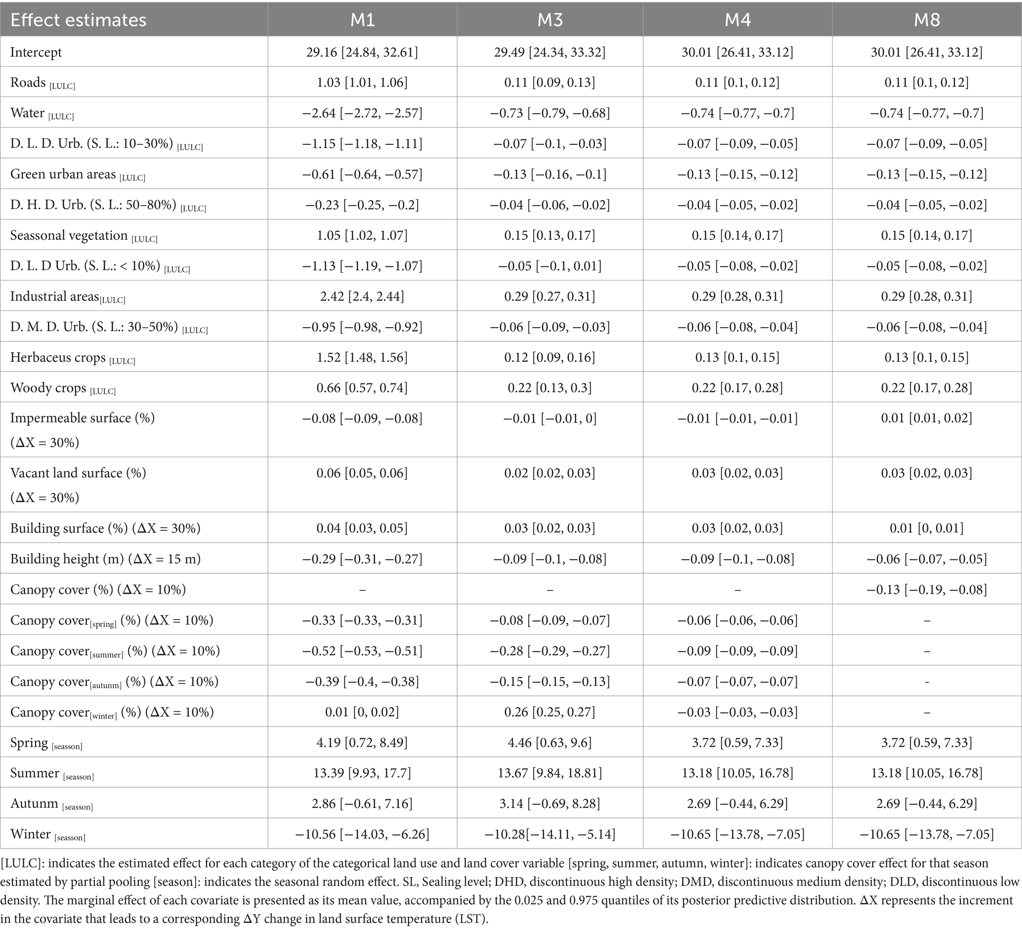
Table 1. Comparison of estimated effects across models.

The inclusion of SPDE effects in the structure of the BHM results in a general reduction of the estimated magnitudes for the effects. Despite this reduction, the directionality of the covariate effects on LST remains consistent across models. An exception is observed in the effect of impervious surface cover, where M4 estimates a negative relationship, while model M8 indicates a positive effect. The inclusion of a temporal effect through a separable space–time model (i.e., moving from a purely spatial model, M3, to a space–time model, M4), or the incorporation of an SVC effect once a spatial or space–time component is already present (M8), does not substantially modify the posterior estimates of the fixed effects.

Given the z-score standardization of the continuous covariates and the selection of “Continuous Urban Fabric (s.l. >80%)” as the reference category for the LULC covariable, the model intercept represents observational units characterized by this specific land use type and average values for all continuous covariates. Accordingly, and under ceteris paribus conditions (i.e., holding all other covariates constant), the land use types “Road Areas,” “Seasonal Vegetation or Bare Ground,” “Industrial Areas,” “Herbaceous Crops” and “Woody Crops” exhibit, on average, higher LST relative to the reference category. As expected, “Industrial Areas” show the highest marginal LST among all LULC categories considered. LULC associated with lower average LST than “continuous urban fabric” include: “water surfaces,” “green urban areas,” “discontinuous high-density urban fabric (s.l. 50–80%),” “discontinuous medium-density urban fabric (s.l. 30–50%)” and “discontinuous low-density urban fabric (s.l. <10%).” Among these, “water surfaces” show the most pronounced LST difference relative to continuous urban fabric, with estimated average differences of approximately −0.75 °C. “Green urban areas” exhibit the second-largest difference in LST in models M3–M8.

For the compositional variables related to impervious surface, building-covered surface, and vacant land surface, all four models estimate effects with a high probability, as indicated by 95% credibility intervals not including zero, but with limited practical significance due to the small magnitude of the estimates. Observational units with a higher fraction of vacant or building surface are associated with higher LST values, regardless of the LULC category they belong to. Contrary to expectations, M4 estimates a negative relationship between impervious surface fraction and LST, whereas model M8 estimates a positive relationship.

Regarding the influence of canopy cover on LST, i.e., the linear cooling capacity effect on LST associated with an increase in tree canopy coverage within an observational unit, there is substantial variation across seasons and between models. In the case of M8, only the global effect of canopy cover is presented, since models incorporating SVC structures typically model the coefficient as the sum of a global effect (an average parameter for the entire study area) and the SVC term that captures local deviations from this mean, presented in later sections. According to M8, a 10% increase in canopy cover per 900 m² observational unit, under ceteris paribus conditions, is associated with an average decrease in LST of −0.13 °C [−0.19 °C, −0.08 °C]. For M4, a drastic reduction in the estimated cooling capacity is observed, with a negative effect estimated with 95% credibility. However, its magnitude is low, with an average LST decrease of 0.03 °C per 10% increase in canopy cover during winter, and a maximum decrease of 0.09 °C per 10% increase observed during summer.

3.3 Hyperparameter estimates

Increasing model complexity results in a decrease in the standard deviation of the gaussian likelihood (Table 2), primarily due to the greater variability captured by the linear predictor. As observed in the canopy cover effect estimates reported in Table 1, when SPDE effect is included, there is a decrease in the standard deviation of the varying slope effect for canopy cover. The posterior mean of the standard deviation for the seasonal effect-generating distribution is similar across models. However, in the case of M4, a greater increase, particularly in the 97.5% quantile, is observed. This may be attributed to the high flexibility introduced by the i.i.d. estimation of the SPDE, which allows the SPDE effect to capture more specific variation from each seasson, thereby making the estimation of the seasonal effect more challenging. Model M8 seasonal effect exhibits a slightly lower average standard deviation, potentially due to the inclusion of the SVC effect, which may be capturing variability that would otherwise be captured by the seasonal effect. M8 shows higher values estimated than M4 for both the range and marginal standard deviation, likely because the SPDE effect in this model is capturing variability at a broader spatial scale due to the concurrent inclusion of the SVC effect. For the SVC effect, the estimated range suggests a localized influence within approximately 200 meters. Its marginal standard devitation indicates the existence of geographic heterogeneity in the relationship between canopy cover and LST.

Table 2

Table 2. Comparison of posterior distributions of hyperparameters across models.

3.4 Predicted spatial patterns of land surface temperature

Model M8 effectively captures and reconstructs the observed spatial pattern of LST for each season, displaying relatively low prediction uncertainty and a narrow residual range. Results for M8 are presented as the observed LST values along with the mean, 2.5, and 97.5% quantiles of the posterior distribution of the linear predictor; prediction uncertainty, expressed as the difference between quantiles; and residuals for spring, summer, autumn, and winter (Figures 2–5). For comparison purposes regarding predictive performance across models M1, M3, M4, and M8, Supplementary Figures S.6–S.8 show the predictions, uncertainties, and residuals disaggregated by season.

Figure 2

Figure 2. Model M8 results for the spring season. (A) Observed mean Land Surface Temperature (LST) values during spring; (B) Posterior mean of the linear predictor; (C) Posterior 2.5% quantile of the linear predictor; (D) Posterior 97.5% quantile of the linear predictor; (E) Prediction uncertainty, defined as the difference between the 97.5 and 2.5% quantiles; and (F) Residuals, calculated as the difference between observed LST values and the posterior mean of the linear predictor. All maps are represented in the EPSG:25830 coordinate reference system.

Figure 3

Figure 3. Model M8 results for the summer season. (A) Observed mean Land Surface Temperature (LST) values during summer; (B) Posterior mean of the linear predictor; (C) Posterior 2.5% quantile of the linear predictor; (D) Posterior 97.5% quantile of the linear predictor; (E) Prediction uncertainty, defined as the difference between the 97.5 and 2.5% quantiles; and (F) Residuals, calculated as the difference between observed LST values and the posterior mean of the linear predictor. All maps are represented in the EPSG:25830 coordinate reference system.

Figure 4

Figure 4. Model M8 results for the autumn season. (A) Observed mean Land Surface Temperature (LST) values during autumn; (B) Posterior mean of the linear predictor; (C) Posterior 2.5% quantile of the linear predictor; (D) Posterior 97.5% quantile of the linear predictor; (E) Prediction uncertainty, defined as the difference between the 97.5 and 2.5% quantiles; and (F) Residuals, calculated as the difference between observed LST values and the posterior mean of the linear predictor. All maps are represented in the EPSG:25830 coordinate reference system.

Figure 5

Figure 5. Model M8 results for the winter season. (A) Observed mean Land Surface Temperature (LST) values during winter; (B) Posterior mean of the linear predictor; (C) Posterior 2.5% quantile of the linear predictor; (D) Posterior 97.5% quantile of the linear predictor; (E) Prediction uncertainty, defined as the difference between the 97.5 and 2.5% quantiles; and (F) Residuals, calculated as the difference between observed LST values and the posterior mean of the linear predictor. All maps are represented in the EPSG:25830 coordinate reference system.

Both M4 and M8 successfully capture the smoothed spatial pattern of LST distribution (Supplementary Figure S.6). These advanced models adequately represent the full range of observed LST values for each season, avoiding the constrained predictions around mean values that characterize simpler modeling approaches.

The highest uncertainty among M4 and M8 across seasons for the linear predictor reaches 1.85 °C (Supplementary Figure S.7). The spatial uncertainty patterns in both models are primarily driven by the mesh used in the modeling process, a common feature of INLA-SPDE models. Both M4 and M8 provide realistic uncertainty estimates that appropriately capture the observed variations in LST, as evidenced by their respective p-LP-HPDI values in Supplementary Table S.1.

The spatial pattern of residuals demonstrates the effectiveness of both M4 and M8 in generating reliable predictions for the study area (Supplementary Figure S.8). Both models display a spatial residual pattern tightly centered around zero, with the main deviations localized in the southwest of the study area. Differences in the spatial residual patterns between M4 and M8 are minimal, and importantly, no structured spatial patterns emerge in either model, indicating their success in capturing the underlying spatial processes. This absence of systematic residual patterns confirms that both approaches effectively model LST across seasons.

3.5 Spatially varying coefficient model effect estimates

The spatial pattern of the local effect estimates of canopy cooling capacity on LST (hereinafter referred to as local effects) is presented in Figure 6. These local effects were computed as the sum of the posterior distribution of the global canopy cover effect and the spatially varying deviations estimated for each observational unit through the SVC component. Mathematically, the units of the effects are reported as the variation in LST for a 10% increase in tree canopy cover. The spatial pattern of the local effect estimates shows high spatial variability, especially when considering the representation of the quantiles (Figures 6A–C). It is important to note that areas with higher localized effects are associated with high uncertainty, reaching up to 3 °C of LST cooling (Figure 6D). These areas are generally linked to regions with low canopy cover and are primarily located in the western part of the study area, coinciding with the airport area, the northwest corresponding to significant vacant land zones, and the southern and southeastern areas related to the Guadalhorce river mouth and port areas, respectively. According to the estimates, for areas with a 95% probability of presenting a localized cooling effect different from zero (Figure 6E), zones with high-magnitude estimates continue to be significant (Figure 6F).

Figure 6

Figure 6. Local effect estimates of canopy cooling capacity as variation in land surface temperature resulting from a 10% increase in tree canopy cover, calculated as the sum of the posterior distributions of the global effect for canopy cover effect and the local deviations per observational unit estimated by the SVC effect. (A) Posterior mean; (B) Posterior quantile 2.5%; (C) Posterior quantile 97.5%; (D) Posterior uncertainty as the difference between the 97.5 and 2.5% quantiles; (E) Significance, understood as local effect estimates whose 95% credibility intervals do not contain zero, i.e., estimates with a 95% probability of being non-zero. Negative and positive indicate the direction of the relationship; (F) Posterior mean of the local effects for observational units whose effects are estimated as significant.

Local effect estimates of canopy cooling capacity are also represented according to LULC type (Figure 7), and their spatial pattern is shown in Supplementary Figure S.9. Considering the uncertainty in the estimation of the SVC effects, represented in the statistical distributions of the population of significant effects in the study area through the mean and the 2.5 and 97.5% quantiles of the posterior distribution of the local effects, it is determined that, firstly, vacant lands, and secondly, green spaces, exhibit the greatest variability in local cooling effects (Figure 7). Distributions of posterior metrics for local effects for vacant lands display greater differences than those for green urban areas or areas with over 25% canopy cover (hereinafter referred as wooded areas), as reflected by their lower overlap in distributions. Specifically, the distribution of local effects in vacant lands shows an average cooling of −0.28 °C, with a 50% coverage interval (CI) of −1.39 °C to 0.71 °C, and 95% CI of −3.34 °C and 2.47 °C. In green urban areas, the mean of the local effects is −0.16 °C, with a 50% CI of −0.68 °C to 0.25 °C and a 95% CI of −2.54 °C to 1.57 °C. In contrast, wooded areas show less heterogeneous and lower-magnitude local effects compared to areas the other areas, contrary to expectations. The distribution of local effects is characterized by an average of −0.09 °C, a 50% CI ranging from −0.254 °C to −0.06 °C, and a 95% CI spanning from −0.496 °C to 0.318 °C.

Figure 7

Figure 7. Statistical distribution for the population of significant posterior mean, quantile 2.5%, and quantile 97.5% values of local effect estimates. The distributions are presented globally for all observations (n = 95.349) and depending on whether the units have more than 25% canopy cover (n = 10,677), are in urban green spaces (n = 5,309), or areas with more than 30% vacant land surface (n = 20,525). The box-plots are represented only for the statistical distribution of posterior means, and thus the X-axis is defined by their values. To improve visualization, the second plot shows zoomed-in distributions constrained to the 10th and 90th quantiles, calculated over the vacant lands distribution, as it exhibits the highest dispersion.

4 Discussion

The potential of urban trees to regulate temperature is widely acknowledged, with forested green spaces exhibiting lower temperatures compared to non-treed areas (Bowler et al., 2010; Gago et al., 2013; Schwaab et al., 2021). Trees mitigate the urban heat primarily through shading and transpiration, with the magnitude of these effects largely depending on tree-specific traits (Rahman et al., 2020). The effectiveness of these cooling mechanisms varies across space and time (Alonzo et al., 2021) and interacts with other components of the built environment (Tsin et al., 2016; Ziter et al., 2019).

In situ studies of air temperature cooling associated with canopy cover show mixed results, particularly depending on the spatial scale or buffer radius considered around temperature measurement points. Ziter et al. (2019), in Madison, Wisconsin, observed a non-linear decrease in air temperature with increasing canopy cover. Their findings indicated a mean air temperature reduction of 0.7 °C when increasing canopy cover from 0 to 100% within a 10 m radius, compared to a 1.3 °C decrease at a 30 m radius, and >1.5 °C when using 60- or 90-m radii. Similarly, Ettinger et al. (2024), working in South Tacoma, Washington, found a reduction of 0.01 °C per 1% increase in field-measured canopy within 10 m. Locke et al. (2024), in New Haven, Connecticut, determined that a 100% increase in tree canopy cover resulted in air temperature reductions of approximately 0.375 °C between 8:00 and 11:00, and 0.75 °C between 11:00 and 14:00, with no statistically significant effects observed after 14:00, all within a 10 m radius. Under a 90 m buffer, the temperature reductions were more substantial: −1.62 °C at midday, −1.19 °C in the afternoon, and −1.15 °C in the morning for a change from 0 to 100% canopy cover. The increased magnitude of cooling effects observed at larger spatial scales may reflect the influence of confounding variables, such as urban geometry or broader atmospheric processes. These factors could potentially lead to overestimations of tree canopy cooling effects, as cooling effects are expected to be more detectable at smaller buffer distances, where temperature measurements occur closer to the actual tree cover and its direct influence.

Regarding high-resolution LST studies, available results are more limited. Bartesaghi-Koc et al. (2020), in Sydney, Australia, observed LST differences of up to 12 °C depending on their proposed typology of green infrastructure. However, they did not conduct a statistical analysis to assess the marginal effect associated with tree canopy cover increase. Ossola et al. (2021), in Adelaide, Australia, found that tree canopy cover had no significant effect on LST at the suburb scale. When analyzing the relationship using buffers around building footprints, they observed an approximate decrease of 0.3 °C per 10% increase in tree canopy cover at a 30 m radius. This effect was reduced to less than 0.1 °C for 60 m buffers and was not detectable at 90 m.

To extend the estimation of tree canopy cooling effects to broader spatial extents, numerous studies have employed satellite-derived LST, either directly or as part of a two-step modeling workflow to estimate air temperature, across various spatial scales (e.g., city-wide, census tracts, urban blocks, grid cells). These studies consistently report average cooling effects across the study area. At the city scale, in a review analyzing air temperature reductions from street trees, it was found that a 10% increase in canopy cover could reduce air temperature by an average of 0.3 °C (Krayenhoff et al., 2021). Schwaab et al. (2021) estimated LST differences using GAMs, comparing predicted LST under a hypothetical scenario of 0% tree canopy cover with those under 100% cover. They reported LST reductions ranging from 0 °C to 4 °C across Southern European regions. Marando et al. (2022) found that air temperature reductions, modeled using LST, ranged from −2.9 °C to 0.4 °C across European Functional Urban Areas as a result of increased canopy cover. Chakraborty et al. (2022) estimated an average LST reduction ranging from 0.3 °C to 1.8 °C, depending on the urban afforestation scenario implemented across 81 cities. Iungman et al. (2023) developed a two-step regression approach to estimate potential cooling capacity, first by quantifying LST reduction due to urban trees and then converting that to air temperature effects. They estimated that achieving a 30% tree canopy cover could cool European cities by 0.4 °C. Studies at finer spatial units also report similar or even smaller effect sizes than those estimated at the city scale. McDonald et al. (2024), working at the block scale in the United States, estimated a reduction of 0.37 °C ± 0.014 °C in median summer air temperature when increasing tree canopy cover to 40%. Shui et al. (2025), analyzing 2,230 cities and counties in China, estimated a reduction in LST ranging from 0.038 °C to 0.144 °C per 1% increase in tree canopy cover, without specific focus on urban trees.

At the grid scale, Kong et al. (2014), in Nanjing, China, observed reductions in LST ranging from 0.61 °C to 0.87 °C for every 10% increase in tree canopy cover, depending on the grid size, and larger reductions were associated with coarser grids. These estimations were performed without controlling for additional factors influencing LST distribution and without considering the effects of spatial autocorrelation. Similarly, Hou and Estoque (2020), in Hangzhou, China, estimated LST reductions of 0.284 °C to 0.292 °C per 10% increase in canopy cover using simple linear regression models. Rogan et al. (2013) estimated that 200 × 200 m grid cells with 10% less tree cover exhibited LST that were, on average, 0.7 °C higher. In Mediterranean environments, Godinho et al. (2016) reported a 0.64 °C decrease in LST per 10% increase in canopy cover. In Addis Abeba, Ethiopia, Feyisa et al. (2014) found a 0.2 °C reduction in LST per 10% increase in canopy cover within urban green spaces. Using machine learning, Yuan et al. (2021) estimated a maximum cooling of 0.8 °C with 64% canopy cover, while Logan et al. (2020) reported daytime cooling ranging from 1.5 to 6.5 °C for a 40% increase in canopy cover, showing a strong linear pattern, both using Landsat 8 pixel resolution.

The global cooling estimates obtained in this study fall on the lower end of the range reported in the literature. Based on model M3 estimates (excluding M1 due to poor model fit and predictive capacity, and excluding M4 due to suspected spatial confounding, discussed later), an LST reduction of −0.28 °C [−0.29, −0.27] is observed for every 10% increase in tree canopy cover during summer. Part of the observed differences with prior studies can be attributed to model structure. Our models included a wide range of covariates known to influence LST, as well as random effects to account for spatial autocorrelation and unmeasured variables. In contrast, many of the studies discussed above used simple univariate linear regressions, without random effects. Neglecting these dependencies can lead to overly narrow credibility intervals and biased estimates of the relative importance of model estimates (Banerjee et al., 2014). The Mediterranean climate of the study area and its location as a coastal city may also contribute to the reduced cooling capacity observed. This diminished effect may stem from lower evapotranspiration rates due to water stress, which limit trees’ ability to dissipate heat through latent flux (Schwaab et al., 2021). Nevertheless, this should be further investigated, as urban trees may be regularly irrigated. Coastal cities also experience less intense UHI effects compared to inland cities due to the moderating influence of oceanic airflow, which reduces thermal extremes (Naserikia et al., 2022). Consequently, the inland-coastal LST gradients are smoother, and diurnal variability in LST is smaller in coastal regions. This homogenizing effect of coastal proximity may reduce the contrast in LST between tree covered and artificial surfaces, leading to lower estimates of tree canopy cooling capacity. Nevertheless, the estimated values in this study remain consistent with those reported in cities with comparable climatic conditions.

Urban environments often exhibit considerable heterogeneity in terms of infrastructure, urban geometry, vegetation cover, and microclimates. The complexity of these settings can lead to spatial variation in the relationship between tree canopy cover and LST (Tsin et al., 2016; Hallar et al., 2021; Kelly-Turner et al., 2022). Accounting for these differences in canopy cooling effects is crucial for urban planning, environmental management, and climate studies, as it suggests that strategies aimed at mitigating heat through increased canopy cover should be tailored to local conditions. In the literature, most studies that explore this spatial variability in the canopy–LST relationship have employed GWR, often using the coverage of green spaces rather than directly measuring urban tree canopy cover (e.g., Chen and Lin, 2021; Li et al., 2021; Liu et al., 2022). Francis et al. (2023) estimated GWR coefficients ranging from −2.36 to 2.06 for the relationship between canopy cover and LST at the block scale in Chicago, without accounting for factors other than average canopy height. The authors did not specify whether covariates and response variables were standardized, or whether canopy cover was included in the model as a percentage or proportion, limiting the interpretability and comparability of the coefficients. Nevertheless, these authors emphasize “the heterogeneity of Chicago’s census blocks whereby depending on the local environmental conditions, simply adding more trees in some locations may not result in reduced LST,” highlighting the importance of conducting localized estimates.

In the present study, an SVC model is employed, allowing the effect of tree canopy cover on LST to vary spatially. The inclusion of the SVC effect, once the SPDE effect is also accounted for (M8), resulted in worse predictive performance compared to models that did not include SVC (M4). This pattern is commonly reported across fields where the application of SVC models is well established (Brodie et al., 2020; Thorson et al., 2023). However, as highlighted by Thorson et al. (2023), the value of SVC models often lies in the nuanced descriptions of processes they can capture, given their ability to model context-dependent covariate responses.

The local effects, for the population of observational units with 95% CI that do not include zero, were estimated to range between [−3.34 °C, 2.47 °C] in vacant lands, [−2.54 °C, 1.57 °C] in green urban spaces, and [−0.496 °C, 0.318 °C] wooded areas. Several hypotheses may help explain these results, beyond the influence of the local characteristics of each observational unit that may modulate tree canopy cooling effects.

1. (1) Saturation Effect in Wooded Areas. Estimated effects in wooded areas were lower than in other land use types, potentially indicating a saturation effect. That is, beyond a certain threshold, additional increases in canopy cover may yield diminishing returns in terms of cooling, resulting in effect estimates that are close to zero or even slightly positive. However, this hypothesis is not consistently supported by existing literature. For instance, Ziter et al. (2019) found that increasing canopy cover from 0 to 40% within a 90-meter radius produced negligible changes in air temperature, whereas increasing cover from 40 to 80% led to approximately 1 °C of cooling, suggesting that greater canopy density may, in fact, enhance cooling effects. Nonetheless, it is important to distinguish between the processes by which tree canopy influences air temperature and LST. While air temperature is more strongly affected by airflow and convective processes, LST is primarily reduced through surface shading (Li et al., 2024). Therefore, it is plausible that once a certain canopy cover threshold is surpassed, where maximum shading has already been achieved, further increases in canopy may not lead to additional LST reductions. In such cases, the marginal effect of increasing canopy becomes negligible, as additional coverage does not significantly enhance surface shading.

2. (2) Greater marginal cooling in vacant lands. Vacant lands often lack significant tree cover and typically exhibit higher baseline LST due to increased solar exposure and heat retention by bare soils. Therefore, the addition of tree canopy in such areas might yield a more pronounced cooling effect, as it introduces shading and evapotranspiration where it was previously absent or minimal. However, Ziter et al. (2019) also noted that areas composed primarily of grassy or low vegetation experienced a smaller cooling benefit when canopy cover increased from 0 to 40% (~0.3 °C), while an increase from 40 to 80% resulted in ~0.8 °C of additional cooling. This suggests that areas dominated by low or seasonal vegetation may require higher canopy densities to achieve effective shading, possibly due to the need to reach higher leaf area indices as suggested by the authors.

3. (3) Influence of surrounding environment. Given the spatial resolution of the pixels used in the analysis, vacant lands, green spaces, and wooded areas are likely to be surrounded by areas with similar land cover. As a result, a vacant land classified pixel is generally embedded in an area with high LST, while green spaces and wooded pixels tend to be surrounded by areas with lower LST. Since the estimation of SVCs is spatially smoothed based on a Gaussian Field with a Matérn covariance structure, the localized effect is influenced by the local relationships in the surrounding environment. Pixels in high-LST areas tend to exhibit higher magnitude local effects, while those in lower-LST surroundings may exhibit reduced magnitudes. This spatial dependence may help explain the broader ranges of estimated effects in areas with lower canopy cover.

The consideration of all the aforementioned hypotheses would require the formulation of causal statements, which we strongly reject. Unlike other authors, such as Francis et al. (2023), we also refrain from using SVCs as a tool for delineating or prioritizing areas for urban tree planting based on the optimization of localized cooling estimates. This decision is based on several key factors, which we believe carry significantly more weight in explaining the results than the physically plausible hypotheses previously discussed.

(1) Detection challenges and model artifacts across the canopy cover gradient. The SVC estimates reveal methodological challenges that arise across the full spectrum of canopy cover conditions, leading to coefficient instability that can produce counterintuitive results. In wooded land pixels with high tree canopy cover, the localized effect of increasing canopy may be challenging to detect at the spatial resolution of Landsat LST, due to the high existing tree canopy cover creating a saturation effect where additional vegetation provides diminishing marginal cooling benefits. Conversely, in areas with very low canopy cover, the low tree canopy coverage limits the model’s ability to estimate the local relationship between tree canopy coverage and LST, as the thermal signal remains dominated by the underlying substrate properties (bare soil, concrete, impervious surfaces, etc.) rather than the limited vegetation present. The counterintuitive warming effects observed in some vacant lands and areas with minimal canopy cover (e.g., up to 2.47 °C positive coefficients) represent methodological artifacts rather than genuine biophysical processes. These artifacts could arise from the model’s inability to isolate the cooling effect of sparse vegetation within thermally extreme environments, where individual trees contribute minimally to the 30-meter pixel scale. It is also important to note that the thermal information is originally measured at 100 m resolution and subsequently resampled by USGS to 30 m, which further complicates detection in areas with low tree density. Additionally, edge effects can cause the model to conflate the warming influence of surrounding impervious surfaces with the vegetation signal when canopy cover falls below critical detection thresholds, due to SVC being based on spatial proximity. These limitations across both high and low canopy cover extremes contribute to the wide range observed in localized effect estimates, emphasizing that SVC results must be interpreted within the context of Landsat LST’s spatial resolution constraints and the underlying thermal heterogeneity of urban environments.

(2) Spatial confounding represents a well-documented phenomenon in spatial regression models that arises when spatial random effects are not independent of covariates or other random effects, as first identified by Clayton et al. (1993) and which has generated substantial research interest recently (Hui et al., 2024; Urdangarin et al., 2024; Gilbert et al., 2024; Lamouroux et al., 2025). Gilbert et al. (2024) identify four main sources of spatial confounding: (i) omitted confounder bias, occurring when unmeasured spatially structured variables influence both exposure and outcome; (ii) regularization bias, stemming from finite-sample bias in models using flexible regression functions such as splines or Gaussian processes to control spatial dependencies; (iii) random effect collinearity, resulting from correlation between spatially dependent random effects and covariates, altering fixed-effect estimates; and (iv) concurvity, complicating estimation when exposure closely follows smooth spatial functions, particularly with additional smooth spatial functions in the model.

As noted by Dupont et al. (2023), spatial confounding is particularly problematic when both random effects exhibit smooth or similar spatial patterns, as their collinearity prevents the distinction of each individual effect. Doser et al. (2024) observed that confounding can occur between the SPDE effect and the SVC, particularly when working with modestly sized datasets (e.g., around 500 data points), which may potentially lead to misleading conclusions. In our case, examination of Supplementary Figures 10, 11 reveals clear similarities between the spatial patterns of the residuals from model M4, defined as the difference between observed Land Surface Temperature values and the posterior mean of the linear predictor, and the posterior mean of the SVC effects estimated by model M8. A moderate negative linear correlation (r = −0.42) indicates that areas where M4 overestimates LST tend to correspond to negative SVC effects in M8, and vice versa, reflecting a moderate degree of spatial confounding. In such cases, the spatially varying coefficient component tends to absorb systematic error patterns not captured by the linear term, leading to compensatory negative or positive values in the SVC estimates.

Thus, even with a large dataset (n = 381,396) and the use of meshes with different characteristics for the SPDE and SVC components, we recommend interpreting the SVC effect estimates with caution, despite the correlation indicating only a moderate degree of confounding. Although various methods have been proposed to address spatial confounding, recent studies caution that many of these approaches may produce counterintuitive or unreliable results. For instance, Khan and Calder (2022) demonstrate that several popular strategies may underperform, while Zimmerman and Ver Hoef (2022) classify some of them as “bad statistical practice.” Despite these concerns, spatial confounding remains a critical issue for future research, particularly in models incorporating SPDE effects, and should be carefully considered in both model development and interpretation. Ongoing debates include whether orthogonalization between spatio-temporal random effects matrices should be applied globally or at each time step, and how this should be implemented in multivariate or multiple data currency contexts (Hui et al., 2024). Recent advances in R-INLA are actively exploring the implementation of tools to mitigate spatial confounding in geostatistical applications (Lamouroux et al., 2025), making it increasingly accessible to practitioners. Continued research is needed to assess the performance, limitations, and optimal application scenarios for the various methods proposed to address spatial confounding, including restricted spatial regression (Khan and Calder, 2022), geoadditive structural equation models (gSEM) and Double Spatial Regression (DSR) (Wiecha et al., 2025), Spatial+ (Dupont et al., 2022), Spatial+ 2.0 (Urdangarin et al., 2024), regularized principal spline functions (Zaccardi et al., 2025), Transformed Gaussian Markov Random Fields (TGMRF) (Prates et al., 2015), and approaches grounded in instrumental variable frameworks (Woodward et al., 2024). Evaluating the stability of estimates across these methods may further clarify whether results obtained from SVC reflect true ecological processes or are artifacts of the particular approach chosen to mitigate spatial confounding.

(3) Residual pattern absorption by the SVC. The poorer performance observed after including the SVC effect may be related to the model’s inability to properly estimate the process of interest, with the SVC instead capturing local residual characteristics, as further suggested by spatial confounding. All environmental or urban features not explicitly included in the model, remaining as residual variation, may cause the SVC to act as a compensatory mechanism for these missing effects. Although the purpose of the SVC is to account for spatial heterogeneity, part of this heterogeneity stems from omitted covariates, while another part reflects genuine variation in the canopy cooling effect (i.e., the process of interest), potentially driven by interactions with multiple factors. SVCs cannot disentangle these two sources of variation. Therefore, in some observational units, local variations in the canopy’s effect on LST may be correctly modeled, while in others, the estimated effect may primarily reflect a compensation for the model’s inability to account for the area’s specific characteristics. This issue is evident both in the present study and in Francis et al. (2023), where, in their estimation of the interaction between canopy area and tree height, port areas emerged as those where canopy contributes most negatively to cooling. This is likely an estimation artifact, with the negative coefficient being influenced by the inclusion or proximity of water pixels, whose effects were not properly accounted for in either study, beyond a categorical variable in the present article. Similarly, as shown in Figure 6H, areas with strongly positive local effects appear to correspond to surfaces with very high albedo, again suggesting an effect driven by the omission of covariates and the absorption of residual patterns by the SVC.

Our findings reveal that planting strategies must evolve beyond simple canopy percentage targets to embrace a comprehensive, trait-based approach that maximizes the cooling potential and resilience of urban forests considering the micro-scale variability. This comprehensive perspective aligns with growing evidence demonstrating the importance of multifunctional and site-specific approaches in urban green infrastructure design for increasing urban areas livability. Recent research has established that government policies and heritage tree protection ordinances can significantly increase urban tree canopy coverage, with municipalities implementing these measures showing up higher canopy coverage than those without protections (Hilbert et al., 2019). Furthermore, strategic urban species selection frameworks must consider not only cooling capacity but also specific physical traits that optimize other ecosystem services, such as precipitation interception and enhanced infiltration for stormwater management (Dowtin et al., 2023). Moreover, district-level urban livability assessment reveals that spatial features such as population density, green space accessibility, and environmental quality are positively correlated with community health outcomes, emphasizing that urban green design must adopt holistic approaches considering both environmental and human well-being benefits (Chi and Mak, 2021). Thus, our findings enable the consideration and evaluation of local specificities in the provision of cooling ecosystem services by urban tree canopies, accounting for the variability that operates at the local scale, which can be seamlessly integrated with other assessment frameworks for multiple ecosystem services, thereby contributing to the advancement of urban development and green space design that aims to enhance livability and well-being in urban environments.

While our spatially explicit modeling approach demonstrates significant spatial variability in cooling effects across urban environment, these results require careful interpretation due to moderate spatial confounding between SPDE and SVC components. This methodological consideration underscores the importance of integrating our findings with established ecological principles rather than relying solely on model predictions for site-specific interventions. Urban planners should prioritize the strategic selection of tree species based on functional characteristics that optimize ecosystem service delivery under local environmental conditions. Functional traits such as high leaf area index, low hydrophobicity, low inclination angles, and high surface roughness promote rainfall retention by the canopy (Dowtin et al., 2023), while trees with high LAI and wider canopies are associated with the greatest daytime cooling benefits (Sharmin et al., 2023). Urban forestry initiatives should therefore prioritize broad-leaved species, large trunk circumferences, tall shapes, low branch point heights, wide and large crowns, umbrella-shaped shapes, large leaf area density (Li et al., 2025), as these morphological characteristics directly enhance the magnitude of cooling benefits while supporting climate resilience (Esperón-Rodríguez et al., 2022).

The potential of this research lies in its capacity to inform evidence-based urban greening that addresses both environmental and social imperatives, though practitioners must acknowledge the inherent spatial confounding challenges in spatially varying coefficient models when interpreting SVC marginal effects. Achieving Sustainable Development Goal 11 requires addressing inequities in access to ecosystem services provided by urban trees to ensure a fair distribution of environmental benefits across socioeconomic groups (Pereña-Ortiz et al., 2025; Ruiz-Valero et al., 2025). Our spatially explicit modeling framework provides urban planners with valuable insights into the spatial heterogeneity of cooling effects, revealing that context-dependent responses are fundamental to urban forest performance rather than exceptional cases. The sustained delivery of ecosystem services depends less on the absolute number of species and more on the presence of ecologically functional vegetation and the maintenance of interspecific interactions that uphold critical ecological processes (Cardinale et al., 2012; Mace et al., 2012; Isbell et al., 2017). This principle should guide urban forest management toward fostering functional diversity rather than simply increasing tree quantity, ensuring that planting efforts contribute meaningfully to urban livability and climate resilience.

Looking forward, urban planning must integrate climate-adaptive species selection with sophisticated understanding of spatial ecological processes to create resilient urban forests capable of delivering sustained ecosystem services under changing environmental conditions. Urban planning and tree selection strategies must proactively identify and promote genotypes or ecotypes that are best suited to future climatic conditions, thereby ensuring long-term planting success and optimizing ecosystem service returns on investment (Watkins et al., 2021). Traits such as specific leaf area, photosynthetic rate, and water-use strategies determine how trees respond to urban stressors like drought, heat, and pollution, ultimately shaping their capacity to provide key ecosystem services (Esperón-Rodríguez et al., 2020; Cho et al., 2024; Ramachandran et al., 2024).

While spatial confounding between SPDE and SVC components necessitates cautious interpretation of our SVC marginal effects, the broader insights regarding spatial heterogeneity and context-dependency remain robust and valuable for advancing urban forestry practice. This work constitutes a fundamental step toward the integration of all previously described factors, together with urban geometry operating at the micro-scale, that influence the cooling capacity of urban tree canopy. An SVC model within a Bayesian hierarchical framework offers substantial advantages over GWR by providing a statistically more robust and flexible approach. SVC models enable automatic learning of spatial hyperparameters such as the length scale of underlying spatial processes, which is critical for understanding spatial process characteristics, while GWR relies on manual bandwidth selection that is highly sensitive and can produce unstable results. Additionally, the Bayesian approach facilitates uncertainty quantification through complete posterior distributions for both coefficients and out-of-sample predictions. The hierarchical Bayesian framework also permits formal incorporation of prior knowledge and provides a more solid probabilistic foundation for statistical inference. Furthermore, hierarchical models allow the inclusion of additional effects, such as SPDE which a priori enables better segregation of effects associated with local temperature variability from the anisotropy in cooling processes that the SVC aims to estimate, a capability that GWR is inherently limited in addressing. However, more comparative and field validation studies are necessary to fully establish these theoretical advantages in practical applications.

The proposed modeling framework advances a shift away from assigning uniform cooling capacities across entire study areas toward explicitly accounting for micro-scale characteristics that modulate this ecosystem service, thereby enabling more spatially nuanced urban forestry decisions. At the same time, further work should systematically evaluate alternative approaches to mitigate or avoid spatial confounding between SPDE and SVC components to obtain robust SVC marginal effect estimates that can be directly applied to identify locations with cooling deficits and to target strategic canopy enhancement. The transparency of the present study is intended to guide future research by foregrounding spatial confounding as a central methodological consideration in study design and inference. Collectively, this work advances the scientific basis for urban forest management by providing a framework that integrates spatial variability, as micro-scale environmental factors, and cooling service quantification for improved urban canopy planning.

4.1 Limitations and future research directions

While the present study has revealed and estimated the local effects of tree canopy coverage on LST, there are limitations deserving further studies:

1. It is important to note that our findings are based on LST rather than air temperature, and as such, not a direct predictor of human thermal comfort. LST, however, might represent a robust indicator when evaluating heat impacts on humans and cities, and for this reason, this parameter has been used in numerous urban studies. The results underscore the importance of tree cover and its variation at a larger scale. Understanding these differences will be crucial for informing urban planning strategies aimed at improving thermal comfort in urban spaces.

2. The analysis was conducted in a single city, and therefore, climate conditions were not considered. As highlighted in the scientific literature, background climate has a significant impact on surface urban heat (Martilli et al., 2020; Naserikia et al., 2022; Li et al., 2024). An important avenue for future research would be to extend the current study to other cities with varying climatic conditions to assess whether there are differences in the statistical distributions of the local relationship between canopy cover and LST.

3. While the proposed model does not meet the requirements for causal inference, understanding the spatial differences in urban tree cooling potential, taking into account urban characteristics that influence LST, can complement and enhance our understanding of the processes that lead to lower urban LST. Therefore, the results highlight the importance of considering the effects of the surrounding environment on cooling capacities and emphasize the need for localized studies.

5 Conclusion

The urban heat island phenomenon strongly reduces thermal comfort in cities, while urban trees provide essential ecosystem services that can mitigate these conditions. However, cooling benefits are often analyzed at the city scale or assumed to be spatially uniform, overlooking evidence that factors such as urban form, canopy structure, and species composition drive substantial local variability. To date, no work has systematically quantified this spatial heterogeneity within a framework that also addresses uncertainty and other latent processes.

This study advances this field by applying SVC within a BHM to account for the fine-scale differences in cooling capacity. The results reveal pronounced spatial variability but also demonstrate the presence of moderate spatial confounding, warranting caution in interpreting localized effects in areas with canopy cover below 25%, which serves as the threshold used in this study. Future research should evaluate the lower reliability limit for SVC estimation to establish more robust guidelines for different canopy cover conditions. These findings highlight the limitations of uniform canopy targets and call for context-sensitive planning that considers local environmental conditions.

Future initiatives should prioritize trait-based species selection to optimize ecosystem service delivery while ensuring equitable access to cooling. At the same time, the methodological framework developed here provides a foundation for spatially explicit urban forest research, while further refinements are needed to address spatial confounding and strengthen causal inference. Ultimately, this work supports the design of evidence-based greening strategies that enhance both climate resilience and urban livability.

Data availability statement

Publicly available datasets were analyzed in this study. This data can be found at: https://code.earthengine.google.com/; https://centrodedescargas.cnig.es/CentroDescargas/catalogo.do?Serie=FPNOA; https://land.copernicus.eu/en/products/urban-atlas.

Author contributions

AR-V: Visualization, Conceptualization, Investigation, Writing – review & editing, Formal analysis, Software, Data curation, Methodology, Writing – original draft. JP-O: Resources, Visualization, Formal analysis, Conceptualization, Validation, Writing – review & editing, Investigation, Methodology. ÁS-T: Visualization, Resources, Conceptualization, Project administration, Validation, Supervision, Writing – review & editing.

Funding

The author(s) declare that financial support was received for the research and/or publication of this article. AR-V was supported by a pre-doctoral grant financed by the Ministry of Education, Professional Formation and Sport of Spain, in the Program of University Teaching Program (Formacion de Profesorado Universitario, FPU) (FPU22/00067).

Acknowledgments

AR-V, JP-O, and AS-T are part of the research team RNM-262: Biogeography, Diversity and Conservation of Junta de Andalucía, Spain.

Conflict of interest

The authors declare that the research was conducted in the absence of any commercial or financial relationships that could be construed as a potential conflict of interest.

Generative AI statement

The authors declare that no Gen AI was used in the creation of this manuscript.

Any alternative text (alt text) provided alongside figures in this article has been generated by Frontiers with the support of artificial intelligence and reasonable efforts have been made to ensure accuracy, including review by the authors wherever possible. If you identify any issues, please contact us.

Publisher’s note

All claims expressed in this article are solely those of the authors and do not necessarily represent those of their affiliated organizations, or those of the publisher, the editors and the reviewers. Any product that may be evaluated in this article, or claim that may be made by its manufacturer, is not guaranteed or endorsed by the publisher.

Supplementary material

The Supplementary material for this article can be found online at: https://www.frontiersin.org/articles/10.3389/ffgc.2025.1644486/full#supplementary-material

References

Ahmad, J., Sajjad, M., and Eisma, J. (2024). Small unmanned aerial vehicle (uav)-based detection of seasonal micro-urban heat islands for diverse land uses. Int. J. Remote Sens. 46, 119–147. doi: 10.1080/01431161.2024.2391582

Crossref Full Text | Google Scholar

Åkerblom, M., and Kaitaniemi, P. (2021). Terrestrial laser scanning: a new standard of forest measuring and modelling? Ann. Bot. 128, 653–662. doi: 10.1093/aob/mcab111

PubMed Abstract | Crossref Full Text | Google Scholar

Alonzo, M., Baker, M. E., Gao, Y., and Shandas, V. (2021). Spatial configuration and time of day impact the magnitude of urban tree canopy cooling. Environ. Res. Lett. 16:084028. doi: 10.1088/1748-9326/ac12f2

Crossref Full Text | Google Scholar

Alonzo, M., Ibsen, P. C., and Locke, D. H. (2025). Urban trees and cooling: a review of the recent literature (2018 to 2024). Arboric. Urban For. 51:jauf.2025.023. doi: 10.48044/jauf.2025.023

Crossref Full Text | Google Scholar

Aybar, C., Wu, Q., Bautista, L., Yali, R., and Barja, A. (2020). Rgee: an R package for interacting with Google earth engine. J. Open Source Softw. doi: 10.32614/CRAN.package.rgee

Crossref Full Text | Google Scholar

Bachl, F. E., Lindgren, F., Borchers, D. L., and Illian, J. B. (2019). Inlabru: an R package for Bayesian spatial modelling from ecological survey data. Methods Ecol. Evol. 10, 760–766. doi: 10.1111/2041-210X.13168

Crossref Full Text | Google Scholar

Balestra, M., Marselis, S., Sankey, T. T., Çabo, C., Liang, X., Mokroš, M., et al. (2024). Lidar data fusion to improve forest attribute estimates: a review. Curr. Forestry Rep. 10, 281–297. doi: 10.1007/s40725-024-00223-7

Crossref Full Text | Google Scholar

Ballester, J., Quijal-Zamorano, M., Méndez Turrubiates, R. F., Pegenaute, F., Herrmann, F. R., Robine, J. M., et al. (2023). Heat-related mortality in Europe during the summer of 2022. Nat. Med. 29, 1857–1866. doi: 10.1038/s41591-023-02419-z

PubMed Abstract | Crossref Full Text | Google Scholar

Banerjee, S., Carlin, B. P., and Gelfand, A. E. (2014). Hierarchical Modeling and analysis for spatial data. 2nd Edn. New York, NY: Chapman and Hall/CRC.

Google Scholar

Barriopedro, D., Fischer, E. M., Luterbacher, J., Trigo, R. M., and García-Herrera, R. (2011). The hot summer of 2010: redrawing the temperature record map of Europe. Science 332, 220–224. doi: 10.1126/science.1201224

Crossref Full Text | Google Scholar

Bartesaghi-Koc, C., Osmond, P., and Peters, A. (2020). Quantifying the seasonal cooling capacity of ‘green infrastructure types’(GITs): an approach to assess and mitigate surface urban heat island in Sydney, Australia. Landsc. Urban Plan. 203:103893. doi: 10.1016/j.landurbplan.2020.103893

Crossref Full Text | Google Scholar

Bechtel, B., Alexander, P. J., Böhner, J., Ching, J., Conrad, O., Feddema, J., et al. (2015). Mapping local climate zones for a worldwide database of the form and function of cities. ISPRS Int. J. Geo Inf. 4, 199–219. doi: 10.3390/ijgi4010199

Crossref Full Text | Google Scholar

Bowler, D. E., Buyung-Ali, L., Knight, T. M., and Pullin, A. S. (2010). Urban greening to cool towns and cities: a systematic review of the empirical evidence. Landsc. Urban Plan. 97, 147–155. doi: 10.1016/j.landurbplan.2010.05.006

Crossref Full Text | Google Scholar

Brodie, S. J., Thorson, J. T., Carroll, G., Hazen, E. L., Bograd, S., Haltuch, M. A., et al. (2020). Trade-offs in covariate selection for species distribution models: a methodological comparison. Ecography 43, 11–24. doi: 10.1111/ecog.04707

Crossref Full Text | Google Scholar

Cardinale, B. J., Duffy, J. E., Gonzalez, A., Hooper, D. U., Perrings, C., Venail, P., et al. (2012). Biodiversity loss and its impact on humanity. Nature 486, 59–67. doi: 10.1038/nature11148

PubMed Abstract | Crossref Full Text | Google Scholar

Casalegno, S., Anderson, K., Cox, D. T. C., Hancock, S., and Gaston, K. J. (2017). Ecological connectivity in the three-dimensional urban green volume using waveform airborne lidar. Sci. Rep. 7:871. doi: 10.1038/srep45571

PubMed Abstract | Crossref Full Text | Google Scholar

CEO (2024). Difusión de datos catastrales. Available online at: https://www.sedecatastro.gob.es/ (Accessed February 01, 2025).

Google Scholar

Chakraborty, T., Biswas, T., Campbell, L. S., Franklin, B., Parker, S. S., and Tukman, M. (2022). Feasibility of afforestation as an equitable nature-based solution in urban areas. Sustain. Cities Soc. 81:103826. doi: 10.1016/j.scs.2022.103826

Crossref Full Text | Google Scholar

Chapman, S., Watson, J. E., Salazar, A., Thatcher, M., and McAlpine, C. A. (2017). The impact of urbanization and climate change on urban temperatures: a systematic review. Landsc. Ecol. 32, 1921–1935. doi: 10.1007/s10980-017-0561-4

Crossref Full Text | Google Scholar

Chen, T. L., and Lin, Z. H. (2021). Impact of land use types on the spatial heterogeneity of extreme heat environments in a metropolitan area. Sustain. Cities Soc. 72:103005. doi: 10.1016/j.scs.2021.103005

Crossref Full Text | Google Scholar

Cheval, S., Amihăesei, V., Chiţu, Z., Dumitrescu, A., Falcescu, V., Irașoc, A., et al. (2024). A systematic review of urban heat island and heat waves research (1991–2022). Clim. Risk Manag. 44:100603. doi: 10.1016/j.crm.2024.100603

Crossref Full Text | Google Scholar

Chi, Y., and Mak, H. W. L. (2021). From comparative and statistical assessments of liveability and health conditions of districts in Hong Kong towards future city development. Sustainability 13:8781. doi: 10.3390/su13168781

Crossref Full Text | Google Scholar

Cho, A., Dziedzic, N., Davis, A. P., Hanson, C. A., Lee, J., Nunez-Mir, G. C., et al. (2024). Leaf functional traits highlight phenotypic variation of two tree species in the urban environment. Front. Plant Sci. 15:1450723. doi: 10.3389/fpls.2024.1450723

PubMed Abstract | Crossref Full Text | Google Scholar

Clayton, D., Bernardinelli, L., and Montomoli, C. (1993). Spatial correlation in ecological analysis. Int. J. Epidemiol. 22, 1193–1202. doi: 10.1093/ije/22.6.1193

PubMed Abstract | Crossref Full Text | Google Scholar

Coops, N. C., Tompalski, P., Goodbody, T. R., Queinnec, M., Luther, J., Bolton, D. K., et al. (2021). Modelling lidar-derived estimates of forest attributes over space and time: a review of approaches and future trends. Remote Sens. Environ. 260:112477. doi: 10.1016/j.rse.2021.112477

Crossref Full Text | Google Scholar

Crawford, C. J., Roy, D. P., Arab, S., Barnes, C., Vermote, E., Hulley, G., et al. (2023). The 50-year Landsat collection 2 archive. Sci. Remote Sensing 8:100103. doi: 10.1016/j.srs.2023.100103

Crossref Full Text | Google Scholar

Demuzere, M., Hankey, S., Mills, G., Zhang, W., Lu, T., and Bechtel, B. (2020). Combining expert and crowd-sourced training data to map urban form and functions for the continental US. Scientific data 7:264. doi: 10.1038/s41597-020-00605-z

PubMed Abstract | Crossref Full Text | Google Scholar

Domeisen, D. I., Eltahir, E. A., Fischer, E. M., Knutti, R., Perkins-Kirkpatrick, S. E., Schär, C., et al. (2023). Prediction and projection of heatwaves. Nat. Rev. Earth Environ. 4, 36–50. doi: 10.1038/s43017-022-00371-z

Crossref Full Text | Google Scholar

Doser, J. W., Kéry, M., Saunders, S. P., Finley, A. O., Bateman, B. L., Grand, J., et al. (2024). Guidelines for the use of spatially varying coefficients in species distribution models. Glob. Ecol. Biogeogr. 33:e13814. doi: 10.1111/geb.13814

Crossref Full Text | Google Scholar

Dowtin, A. L., Cregg, B. C., Nowak, D. J., and Levia, D. F. (2023). Towards optimized runoff reduction by urban tree cover: a review of key physical tree traits, site conditions, and management strategies. Landsc. Urban Plan. 239:104849. doi: 10.1016/j.landurbplan.2023.104849

Crossref Full Text | Google Scholar

Dupont, E., Marques, I., and Kneib, T. (2023). Demystifying spatial confounding. arXiv preprint arXiv:2309.16861. doi: 10.48550/arXiv.2309.16861

Crossref Full Text | Google Scholar

Dupont, E., Wood, S. N., and Augustin, N. H. (2022). Spatial+: a novel approach to spatial confounding. Biometrics 78, 1279–1290. doi: 10.1111/biom.13656

PubMed Abstract | Crossref Full Text | Google Scholar

Endreny, T. A. (2018). Strategically growing the urban forest will improve our world. Nat. Commun. 9:1160. doi: 10.1038/s41467-018-03622-0

PubMed Abstract | Crossref Full Text | Google Scholar

Esperón-Rodríguez, M., Rymer, P. D., Power, S. A., Challis, A., Marchin, R. M., and Tjoelker, M. G. (2020). Functional adaptations and trait plasticity of urban trees along a climatic gradient. Urban For. Urban Green. 54:126771. doi: 10.1016/j.ufug.2020.126771

Crossref Full Text | Google Scholar

Esperón-Rodríguez, M., Tjoelker, M. G., Lenoir, J., Baumgartner, J. B., Beaumont, L. J., Nipperess, D. A., et al. (2022). Climate change increases global risk to urban forests. Nat. Clim. Chang. 12, 950–955. doi: 10.1038/s41558-022-01465-8

Crossref Full Text | Google Scholar

Ettinger, A. K., Bratman, G. N., Carey, M., Hebert, R., Hill, O., Kett, H., et al. (2024). Street trees provide an opportunity to mitigate urban heat and reduce risk of high heat exposure. Sci. Rep. 14:3266. doi: 10.1038/s41598-024-51921-y

PubMed Abstract | Crossref Full Text | Google Scholar

EEA (2018). Urban atlas land cover/land use 2018 (vector), Europe, 6-yearly, Jul. 2021. Copernicus land monitoring service (CLMS). Copenhagen: European Environment Agency (EEA).

Google Scholar

Fassnacht, F. E., White, J. C., Wulder, M. A., and Næsset, E. (2023). Remote sensing in forestry: current challenges, considerations and directions. Forestry Int. J. Forest Research 97, 11–37. doi: 10.1093/forestry/cpad024

Crossref Full Text | Google Scholar

Feyisa, G. L., Dons, K., and Meilby, H. (2014). Efficiency of parks in mitigating urban heat island effect: an example from Addis Ababa. Landsc. Urban Plan. 123, 87–95. doi: 10.1016/j.landurbplan.2013.12.008

Crossref Full Text | Google Scholar

Finley, A. O. (2011). Comparing spatially-varying coefficients models for analysis of ecological data with non-stationary and anisotropic residual dependence. Methods Ecol. Evol. 2, 143–154. doi: 10.1111/j.2041-210X.2010.00060.x

Crossref Full Text | Google Scholar

Finley, A. O., and Banerjee, S. (2020). Bayesian spatially varying coefficient models in the spBayes R package. Environ. Model. Softw. 125:104608. doi: 10.1016/j.envsoft.2019.104608

Crossref Full Text | Google Scholar

Fotheringham, A. S., Brunsdon, C., and Charlton, M. (2009). Geographically weighted regression. Sage Handb. Spatial Analysis 1, 243–254. doi: 10.4135/9780857020130

Crossref Full Text | Google Scholar

Founda, D., and Santamouris, M. (2017). Synergies between urban Heat Island and heat waves in Athens (Greece), during an extremely hot summer (2012). Sci. Rep. 7:10973. doi: 10.1038/s41598-017-11407-6

PubMed Abstract | Crossref Full Text | Google Scholar

Fox, J., and Weisberg, S. (2019). An R companion to applied regression. Third Edn. Thousand Oaks CA: Sage.

Google Scholar

Francis, J., Disney, M., and Law, S. (2023). Monitoring canopy quality and improving equitable outcomes of urban tree planting using LiDAR and machine learning. Urban For. Urban Green. 89:128115. doi: 10.1016/j.ufug.2023.128115

Crossref Full Text | Google Scholar

Gago, E. J., Roldan, J., Pacheco-Torres, R., and Ordóñez, J. (2013). The city and urban heat islands: a review of strategies to mitigate adverse effects. Renew. Sust. Energ. Rev. 25, 749–758. doi: 10.1016/j.rser.2013.05.057

Crossref Full Text | Google Scholar

Gelfand, A. E., Kim, H. J., Sirmans, C. F., and Banerjee, S. (2003). Spatial modeling with spatially varying coefficient processes. J. Am. Stat. Assoc. 98, 387–396. doi: 10.1198/016214503000170

PubMed Abstract | Crossref Full Text | Google Scholar

Gelman, A., Carlin, J. B., Stern, H. S., Dunson, D. B., Vehtari, A., and Rubin, D. B. (2013). Bayesian data analysis. Cham: Springer.

Google Scholar

Gilbert, B., Ogburn, E. L., and Datta, A. (2024). Consistency of common spatial estimators under spatial confounding. Biometrika 112:070. doi: 10.1093/biomet/asae070

PubMed Abstract | Crossref Full Text | Google Scholar

Godinho, S., Gil, A., Guiomar, N., Costa, M. J., and Neves, N. (2016). Assessing the role of mediterranean evergreen oaks canopy cover in land surface albedo and temperature using a remote sensing-based approach. Applied Geography, 74, 84–94. doi: 10.1016/j.apgeog.2016.07.004

Crossref Full Text | Google Scholar

Gómez-Muñoz, V. M., Porta-Gándara, M. Á., and Fernández, J. (2010). Effect of tree shades in urban planning in hot-arid climatic regions. Landsc. Urban Plan. 94, 149–157. doi: 10.1016/j.landurbplan.2009.09.002

Crossref Full Text | Google Scholar

Gorelick, N., Hancher, M., Dixon, M., Ilyushchenko, S., Thau, D., and Moore, R. (2017). Google earth engine: planetary-scale geospatial analysis for everyone. Remote Sens. Environ. 202, 18–27. doi: 10.1016/j.rse.2017.06.031

Crossref Full Text | Google Scholar

Hallar, A. G., Brown, S. S., Crosman, E., Barsanti, K. C., Cappa, C. D., Faloona, I., et al. (2021). Coupled air quality and boundary-layer meteorology in western US basins during winter: design and rationale for a comprehensive study. Bull. Am. Meteorol. Soc. 102, E2012–E2033. doi: 10.1175/BAMS-D-20-0017.1

PubMed Abstract | Crossref Full Text | Google Scholar

Hastie, T., Tibshirani, R., and Friedman, J. H. (2009). The elements of statistical learning. Cham: Springer.

Google Scholar

Hilbert, D. R., Koeser, A. K., Roman, L. A., Hamilton, K., Landry, S. M., Hauer, R. J., et al. (2019). Development practices and ordinances predict inter-city variation in Florida urban tree canopy coverage. Landsc. Urban Plan. 190:103603. doi: 10.1016/j.landurbplan.2019.103603

Crossref Full Text | Google Scholar

Hou, H., and Estoque, R. C. (2020). Detecting cooling effect of landscape from composition and configuration: an urban heat island study on Hangzhou. Urban For. Urban Green. 53:126719. doi: 10.1016/j.ufug.2020.126719

Crossref Full Text | Google Scholar

Houghton, R. A., House, J. I., Pongratz, J., van der Werf, G. R., DeFries, R. S., Hansen, M. C., et al. (2012). Carbon emissions from land use and land-cover change. Biogeosciences 9, 5125–5142. doi: 10.5194/bg-9-5125-2012

Crossref Full Text | Google Scholar

Hui, F. K. C., Vu, Q., and Hooten, M. B. (2024). Spatial confounding in joint species distribution models. Methods Ecol. Evol. 15, 1906–1921. doi: 10.1111/2041-210x.14420

Crossref Full Text | Google Scholar

Isbell, F., Gonzalez, A., Loreau, M., Cowles, J., Díaz, S., Hector, A., et al. (2017). Linking the influence and dependence of people on biodiversity across scales. Nature 546, 65–72. doi: 10.1038/nature22899

PubMed Abstract | Crossref Full Text | Google Scholar

Iungman, T., Cirach, M., Marando, F., Pereira Barboza, E., Khomenko, S., Masselot, P., et al. (2023). Cooling cities through urban green infra-structure: a health impact assessment of European cities. Lancet 401, 577–589. doi: 10.1016/S0140-6736(22)02585-5

PubMed Abstract | Crossref Full Text | Google Scholar

Kelly-Turner, V., Rogers, M. L., Zhang, Y., Middel, A., Schneider, F. A., Ocón, J. P., et al. (2022). More than surface temperature: mitigating thermal exposure in hyper-local land system. J. Land Use Sci. 17, 79–99. doi: 10.1080/1747423X.2021.2015003

Crossref Full Text | Google Scholar

Khan, K., and Calder, C. A. (2022). Restricted spatial regression methods: implications for inference. J. Am. Stat. Assoc. 117, 482–494. doi: 10.1080/01621459.2020.1788949

PubMed Abstract | Crossref Full Text | Google Scholar

Koenig, K., and Höfle, B. (2016). Full-waveform airborne laser scanning in vegetation studies—a review of point cloud and waveform features for tree species classification. Forests 7:198. doi: 10.3390/f7090198

Crossref Full Text | Google Scholar

Kong, F., Yin, H., James, P., Hutyra, L. R., and He, H. S. (2014). Effects of spatial pattern of greenspace on urban cooling in a large metropolitan area of eastern China. Landsc. Urban Plann. 128, 35–47. doi: 10.1016/j.landurbplan.2014.04.018

Crossref Full Text | Google Scholar

Kovanič, Ľ., Topitzer, B., Peťovský, P., Blišťan, P., Gergeľová, M. B., and Blišťanová, M. (2023). Review of photogrammetric and lidar applications of UAV. Appl. Sci. 13:6732. doi: 10.3390/app13116732

Crossref Full Text | Google Scholar

Krainski, E., Gómez-Rubio, V., Bakka, H., Lenzi, A., Castro-Camilo, D., Simpson, D., et al. (2018). Advanced spatial modeling with stochastic partial differential equations using R and INLA. New York, NY: Chapman and Hall/CRC.

Google Scholar

Krayenhoff, E. S., Broadbent, A. M., Zhao, L., Georgescu, M., Middel, A., Voogt, J. A., et al. (2021). Cooling hot cities: a systematic and critical review of the numerical modelling literature. Environ. Res. Lett. 16:053007. doi: 10.1088/1748-9326/abdcf1

Crossref Full Text | Google Scholar

Lamouroux, J., Geffroy, A., Leblond, S., Meyer, C., and Albert, I. (2025). Addressing spatial confounding in geostatistical regression models: an R-INLA approach. Methods Ecol. Evol. 16, 2082–2097. doi: 10.1111/2041-210X.70106

Crossref Full Text | Google Scholar

Li, Y., Liu, X., Cheshmehzangi, A., Zahed, L. M., and He, B. (2025). Multidimensional factors affecting tree-induced cooling benefits: a comprehensive review. Build. Environ. 282:113242. doi: 10.1016/j.buildenv.2025.113242

Crossref Full Text | Google Scholar

Li, Z., Wu, H., Duan, S., Zhao, W., Ren, H., Liu, X., et al. (2023). Satellite remote sensing of global land surface temperature: definition, methods, products, and applications. Rev. Geophys. 61:777. doi: 10.1029/2022rg000777

Crossref Full Text | Google Scholar

Li, T., Xu, Y., and Yao, L. (2021). Detecting urban landscape factors controlling seasonal land surface temperature: from the perspective of urban function zones. Environ. Sci. Pollut. Res. 28, 41191–41206. doi: 10.1007/s11356-021-13695-y

PubMed Abstract | Crossref Full Text | Google Scholar

Li, H., Zhao, Y., Wang, C., Ürge-Vorsatz, D., Carmeliet, J., and Bardhan, R. (2024). Cooling efficacy of trees across cities is determined by background climate, urban morphology, and tree trait. Commun. Earth Environ. 5, 1–14. doi: 10.1038/s43247-024-01908-4

Crossref Full Text | Google Scholar

Lindenmayer, D. B., and Laurance, W. F. (2016). The ecology, distribution, conservation and management of large old trees. Biol. Rev. 92, 1434–1458. doi: 10.1111/brv.12290

Crossref Full Text | Google Scholar

Lindenmayer, D. B., Laurance, W. F., and Franklin, J. F. (2012). Global decline in large old trees. Science 338, 1305–1306. doi: 10.1126/science.1231070

PubMed Abstract | Crossref Full Text | Google Scholar

Lindgren, F., Rue, H., and Lindström, J. (2011). An explicit link between gaussian fields and gaussian Markov random fields: the stochastic partial differential equation approach. J. R. Stat. Soc. Ser. B Stat Methodol. 73, 423–498. doi: 10.1111/j.1467-9868.2011.00777.x

Crossref Full Text | Google Scholar

Liu, Z., Barlow, J. F., Chan, P. W., Fung, J. C. H., Li, Y., Ren, C., et al. (2019). A review of progress and applications of pulsed doppler wind lidars. Remote Sens 11:2522. doi: 10.3390/rs11212522

Crossref Full Text | Google Scholar

Liu, W., Jia, B., Li, T., Zhang, Q., and Ma, J. (2022). Correlation analysis between urban green space and land surface temperature from the perspective of spatial heterogeneity: a case study within the sixth ring road of Beijing. Sustainability 14:13492. doi: 10.3390/su142013492

Crossref Full Text | Google Scholar

Locke, D. H., Baker, M., Alonzo, M., Yang, Y., Ziter, C. D., Murphy-Dunning, C., et al. (2024). Variation the in relationship between urban tree canopy and air temperature reduction under a range of daily weather conditions. Heliyon 10:e25041. doi: 10.1016/j.heliyon.2024.e25041

PubMed Abstract | Crossref Full Text | Google Scholar

Logan, T. M., Zaitchik, B., Guikema, S., and Nisbet, A. (2020). Night and day: the influence and relative importance of urban characteristics on remotely sensed land surface temperature. Remote Sens. Environ. 247:111861. doi: 10.1016/j.rse.2020.111861

Crossref Full Text | Google Scholar

Lorenzo, N., Díaz-Poso, A., and Royé, D. (2021). Heatwave intensity on the Iberian Peninsula: future climate projections. Atmos. Res. 258:105655. doi: 10.1016/j.atmosres.2021.105655

Crossref Full Text | Google Scholar

Mace, G. M., Norris, K., and Fitter, A. (2012). Biodiversity and ecosystem services: a multilayered relationship. Trends Ecol. Evol. 27, 19–26. doi: 10.1016/j.tree.2011.08.006

PubMed Abstract | Crossref Full Text | Google Scholar

Mannucci, S., Kwakkel, J., Morganti, M., and Ferrero, M. (2023). Exploring potential futures: evaluating the influence of deep uncertainties in urban planning through scenario planning: a case study in Rome, Italy. Futures 154:103265. doi: 10.1016/j.futures.2023.103265

Crossref Full Text | Google Scholar

Marando, F., Heris, M. P., Zulian, G., Udías, A., Mentaschi, L., Chrysoulakis, N., et al. (2022). Urban heat island mitigation by green infrastructure in European functional urban areas. Sustain. Cities Soc. 77:103564. doi: 10.1016/j.scs.2021.103564

Crossref Full Text | Google Scholar

Martilli, A., Krayenhoff, E. S., and Nazarian, N. (2020). Is the urban heat island intensity relevant for heat mitigation studies? Urban Clim. 31:100541. doi: 10.1016/j.uclim.2019.100541

Crossref Full Text | Google Scholar

McDonald, R. I., Biswas, T., Chakraborty, T. C., Kroeger, T., Cook-Patton, S. C., and Fargione, J. E. (2024). Current inequality and future potential of US urban tree cover for reducing heat-related health impacts. NPJ Urban Sustain. 4:18. doi: 10.1038/s42949-024-00150-3

Crossref Full Text | Google Scholar

Miedema-Brown, L., and Anand, M. (2022). Plant functional traits as measures of ecosystem service provision. Ecosphere 13:e3930. doi: 10.1002/ecs2.3930

Crossref Full Text | Google Scholar

Münzinger, M., Prechtel, N., and Behnisch, M. (2022). Mapping the urban forest in detail: from lidar point clouds to 3d tree models. Urban For. Urban Green. 74:127637. doi: 10.1016/j.ufug.2022.127637

Crossref Full Text | Google Scholar

Naserikia, M., Hart, M. A., Nazarian, N., and Bechtel, B. (2022). Background climate modulates the impact of land cover on urban surface temperature. Sci. Rep. 12:15433. doi: 10.1038/s41598-022-19431-x

PubMed Abstract | Crossref Full Text | Google Scholar

NIG (2017). Sistema de Ocupación del Suelo de España de Alta Resolucion [Cartografía Digital]. Málaga. Available online at: https://www.siose.es/siose-alta-resolucion (Accessed February 01, 2025).

Google Scholar

NIG (2022). Plan Nacional de Ortofotografía Aérea (PNOA) / Plan Nacional de Observación del Territorio (PNOT). Available online at: https://pnoa.ign.es/ (Accessed February 01, 2025).

Google Scholar

NIS (2024). Cifras oficiales de población de los municipios españoles en aplicación de la Ley de Bases del Régimen Local (Art. 17). Detalle municipal: Málaga. Población por municipios y sexo. Unidades: Personas. Available online at: https://www.ine.es/dynt3/inebase/index.htm?padre=525 (accessed April 22, 2025).

Google Scholar

Oke, T. R., Mills, G., Christen, A., and Voogt, J. A. (2017). Urban climates. Cambridge: Cambridge university press.

Google Scholar

Ossola, A., Jenerette, G. D., McGrath, A., Chow, W., Hughes, L., and Leishman, M. R. (2021). Small vegetated patches greatly reduce urban surface temperature during a summer heatwave in Adelaide, Australia. Landsc. Urban Plan. 209:104046. doi: 10.1016/j.landurbplan.2021.104046

Crossref Full Text | Google Scholar

Pande, C. B., Egbueri, J. C., Costache, R., Sidek, L. M., Wang, Q., Alshehri, F., et al. (2024). Predictive modeling of land surface temperature (lst) based on Landsat-8 satellite data and machine learning models for sustainable development. J. Clean. Prod. 444:141035. doi: 10.1016/j.jclepro.2024.141035

Crossref Full Text | Google Scholar

Pataki, D. E., Alberti, M., Cadenasso, M. L., Felson, A. J., McDonnell, M. J., Pincetl, S., et al. (2021). The benefits and limits of urban tree planting for environmental and human health. Front. Ecol. Evol. 9:603757. doi: 10.3389/fevo.2021.603757

Crossref Full Text | Google Scholar

Pebesma, E. J. (2004). Multivariable geostatistics in S: the gstat package. Comput. Geosci. 30, 683–691. doi: 10.1016/j.cageo.2004.03.012

Crossref Full Text | Google Scholar

Pereña-Ortiz, J. F., Salvo-Tierra, Á. E., Cozano-Pérez, P., and Ruiz-Valero, Á. (2025). Propagating uncertainty in urban tree trait measurements to estimate socioeconomic inequities in ecosystem service accessibility: a machine learning and simulation framework. Environ. Sustain. Indic. 27:100864. doi: 10.1016/j.indic.2025.100864

Crossref Full Text | Google Scholar

Phelan, P. E., Kaloush, K., Miner, M., Golden, J., Phelan, B., Silva, H. III, et al. (2015). Urban heat island: mechanisms, implications, and possible remedies. Annu. Rev. Environ. Resour. 40, 285–307. doi: 10.1146/annurev-environ-102014-021155

Crossref Full Text | Google Scholar

Prates, M. O., Dey, D. K., Willig, M. R., and Yan, J. (2015). Transformed gaussian markov random fields and spatial modeling of species abundance. Spatial Statistics 14, 382–399. doi: 10.1016/j.spasta.2015.07.004

Crossref Full Text | Google Scholar

Rahman, M. A., Stratopoulos, L. M., Moser-Reischl, A., Zölch, T., Häberle, K. H., Rötzer, T., et al. (2020). Traits of trees for cooling urban heat islands: a meta-analysis. Build. Environ. 170:106606. doi: 10.1016/j.buildenv.2019.106606

Crossref Full Text | Google Scholar

Rajagopal, P., Priya, R. S., and Senthil, R. (2023). A review of recent developments in the impact of environmental measures on urban heat island. Sustain. Cities Soc. 88:104279. doi: 10.1016/j.scs.2022.104279

Crossref Full Text | Google Scholar

Ramachandran, A., Dee, L. E., Hayden, M. T., and Suding, K. N. (2024). Leveraging plant functional traits in the design of nature-based solutions: a research agenda. J. Ecol. 112, 2492–2501. doi: 10.1111/1365-2745.14371

Crossref Full Text | Google Scholar

Roberts, D. R., Bahn, V., Ciuti, S., Boyce, M. S., Elith, J., Guillera-Arroita, G., et al. (2017). Cross-validation strategies for data with temporal, spatial, hierarchical, or phylogenetic structure. Ecography 40, 913–929. doi: 10.1111/ecog.02881

Crossref Full Text | Google Scholar

Robine, J. M., Cheung, S. L. K., Le Roy, S., Van Oyen, H., Griffiths, C., Michel, J. P., et al. (2008). Death toll exceeded 70,000 in Europe during the summer of 2003. C. R. Biol. 331, 171–178. doi: 10.1016/j.crvi.2007.12.001

PubMed Abstract | Crossref Full Text | Google Scholar

Rogan, J., Ziemer, M., Martin, D., Ratick, S., Cuba, N., and DeLauer, V. (2013). The impact of tree cover loss on land surface temperature: a case study of Central Massachusetts using Landsat thematic mapper thermal data. Appl. Geogr. 45, 49–57. doi: 10.1016/j.apgeog.2013.07.004

Crossref Full Text | Google Scholar

Rollinson, C. R., Finley, A. O., Alexander, M. R., Banerjee, S., Dixon Hamil, K. A., Koenig, L. E., et al. (2021). Working across space and time: nonstationarity in ecological research and application. Front. Ecol. Environ. 19, 66–72. doi: 10.1002/fee.2298

Crossref Full Text | Google Scholar

Roussel, J., and Auty, D. (2024). Airborne LiDAR data manipulation and visualization for forestry applications. R package version 4.1.2. Available online at: https://cran.r-project.org/package=lidR (Accessed February 01, 2025).

Google Scholar

Roussel, J. R., Auty, D., Coops, N. C., Tompalski, P., Goodbody, T. R., Meador, A. S., et al. (2020). LidR: an R package for analysis of airborne laser scanning (ALS) data. Remote Sens. Environ. 251:112061. doi: 10.1016/j.rse.2020.112061

Crossref Full Text | Google Scholar

Rue, H., Martino, S., and Chopin, N. (2009). Approximate Bayesian inference for latent gaussian models by using integrated nested Laplace approximations. J. R. Stat. Soc. Ser. B Stat Methodol. 71, 319–392. doi: 10.1111/j.1467-9868.2008.00700.x

Crossref Full Text | Google Scholar

Ruiz-Valero, Á., Cozano-Pérez, P., Ortiz, J. P., Guerrero-Serrano, P. M., and Tierra, Á. E. S. (2025). Tree structural traits as a key element for ensuring socio-economic equitable access to ecosystem services. Trees Forests People 21:100899. doi: 10.1016/j.tfp.2025.100899

Crossref Full Text | Google Scholar

Schwaab, J., Meier, R., Mussetti, G., Seneviratne, S., Bürgi, C., and Davin, E. L. (2021). The role of urban trees in reducing land surface temperatures in European cities. Nat. Commun. 12:6763. doi: 10.1038/s41467-021-26768-w

PubMed Abstract | Crossref Full Text | Google Scholar

Seto, K. C., Güneralp, B., and Hutyra, L. R. (2012). Global forecasts of urban expansion to 2030 and direct impacts on biodiversity and carbon pools. Proc. Natl. Acad. Sci. 109, 16083–16088. doi: 10.1073/pnas.1211658109

PubMed Abstract | Crossref Full Text | Google Scholar

Sharma, G., Morgenroth, J., Richards, D. R., and Ye, N. (2025). Advancing urban forest and ecosystem service assessment through the integration of remote sensing and i-tree eco: a systematic review. Urban For. Urban Green. 104:128659. doi: 10.1016/j.ufug.2024.128659

Crossref Full Text | Google Scholar

Sharmin, M., Tjoelker, M. G., Pfautsch, S., Esperón-Rodríguez, M., Rymer, P. D., and Power, S. A. (2023). Tree traits and microclimatic conditions determine cooling benefits of urban trees. Atmos. 14:606. doi: 10.3390/atmos14030606

Crossref Full Text | Google Scholar

Shojanoori, R., and Shafri, H. Z. M. (2016). Review on the use of remote sensing for urban forest monitoring. Arboric. Urban. For. 42:34. doi: 10.48044/jauf.2016.034

Crossref Full Text | Google Scholar

Shui, C., Shan, B., Li, W., Wang, L., and Liu, Y. (2025). Investigating the influence of land cover on land surface temperature. Adv. Space Res. 75, 2614–2631. doi: 10.1016/j.asr.2024.11.016

Crossref Full Text | Google Scholar

SMA (2025). Agencia Estatal de Meteorología - AEMET. Servicios Climáticos. Valores climatológicos normales 1981-2010, Málaga Aeropuerto. Ministerio para la Transición Ecológica y el Reto Demográfico. Madrid: SMA.

Google Scholar

Stein, M. L. (2014). Limitations on low rank approximations for covariance matrices of spatial data. Spatial Stat. 8, 1–19. doi: 10.1016/j.spasta.2013.06.003

Crossref Full Text | Google Scholar

Sterkenburg, T. F. (2024). Statistical learning theory and Occam’s razor: the core argument. Minds Mach. 35:9703. doi: 10.1007/s11023-024-09703-y

Crossref Full Text | Google Scholar

Thorson, J. T., Barnes, C. L., Friedman, S. T., Morano, J. L., and Siple, M. C. (2023). Spatially varying coefficients can improve parsimony and descriptive power for species distribution models. Ecography 2023:e06510. doi: 10.1111/ecog.06510

Crossref Full Text | Google Scholar

Tsin, P. K., Knudby, A., Krayenhoff, E. S., Ho, H. C., Brauer, M., and Henderson, S. B. (2016). Microscale mobile monitoring of urban air temperature. Urban Clim. 18, 58–72. doi: 10.1016/j.uclim.2016.10.001

Crossref Full Text | Google Scholar

Unal Cilek, M., and Cilek, A. (2021). Analyses of land surface temperature (LST) variability among local climate zones (LCZs) comparing Landsat-8 and ENVI-met model data. Sustain. Cities Soc. 69:102877. doi: 10.1016/j.scs.2021.102877

Crossref Full Text | Google Scholar

UN (2023). Independent Group of Scientists appointed by the secretary-general, global sustainable development report 2023: times of crisis, times of change: science for accelerating transformations to sustainable development. Available online at: https://sustainabledevelopment.un.org/content/documents/24797GSDR_report_2019.pdf (Accessed February 01, 2025).

Google Scholar

UN, (2025). United Nations Trade & Development (UNCTAD) data hub. Total and urban population, annual. Available online at: https://unctadstat.unctad.org/datacentre/dataviewer/US.PopTotal (accessed March 2, 2025).

Google Scholar

USGS (2020). Landsat 8-9 operational land imager / thermal infrared sensor Level-2, collection 2. U.S. Geological Survey. Reston, VI: United States Geological Survey (USGS).

Google Scholar

UIS (2024). Sistema de Información Urbana, SIU 2024. Ministerio de Vivienda y Agenda Urbanba; DG de Vivienda y Suelo. NIPO: 179-24-020-5. Reston, VI: Urban Information System (UIS).

Google Scholar

Urdangarin, A., Goicoa, T., Kneib, T., and Ugarte, M. D. (2024). A simplified spatial+ approach to mitigate spatial confounding in multivariate spatial areal models. Spatial Stat. 59:100804. doi: 10.1016/j.spasta.2023.100804

Crossref Full Text | Google Scholar

Valavi, R., Elith, J., Lahoz-Monfort, J. J., and Guillera-Arroita, G. (2019). BlockCV: an R package for generating spatially or envi-ronmentally separated folds for k-fold cross-validation of species distribution models. Methods Ecol. Evol. 10, 225–232. doi: 10.1111/2041-210X.13107

Crossref Full Text | Google Scholar

Wang, J., Zhou, W., Pickett, S. T. A., and Qian, Y. (2024). A scaling law for predicting urban trees canopy cooling efficiency. Proc. Natl. Acad. Sci. 121:e2401210121. doi: 10.1073/pnas.2401210121

PubMed Abstract | Crossref Full Text | Google Scholar

Watkins, H., Hirons, A. D., Sjöman, H., Cameron, R., and Hitchmough, J. (2021). Can trait-based schemes be used to select species in urban forestry? Front. Sustain. Cities 3:654618. doi: 10.3389/frsc.2021.654618

Crossref Full Text | Google Scholar

Wheeler, D. C., and Calder, C. A. (2007). An assessment of coefficient accuracy in linear regression models with spatially varying coefficients. J. Geogr. Syst. 9, 145–166. doi: 10.1007/s10109-006-0040-y

Crossref Full Text | Google Scholar

Wiecha, N., Hoppin, J. A., and Reich, B. J. (2025). Two-stage estimators for spatial confounding with point-referenced data. Biometrics 81:093. doi: 10.1093/biomtc/ujaf093

PubMed Abstract | Crossref Full Text | Google Scholar

Wood, S. N. (2017). Generalized additive models: An introduction with R. London: Chapman and Hall/CRC.

Google Scholar

Woodward, S. M., Tec, M., and Dominici, F. (2024). An instrumental variables framework to unite spatial confounding methods. arXiv preprint arXiv:2411.10381. doi: 10.48550/arXiv.2411.10381

Crossref Full Text | Google Scholar

Wulder, M. A., Roy, D. P., Radeloff, V. C., Loveland, T. R., Anderson, M. C., Johnson, D. M., et al. (2022). Fifty years of Landsat science and impacts. Remote Sens. Environ. 280:113195. doi: 10.1016/j.rse.2022.113195

Crossref Full Text | Google Scholar

Xu, Y., Wang, T., and Skidmore, A. K. (2025). Fusing aerial photographs and airborne lidar data to improve the accuracy of detecting individual trees in urban and peri-urban areas. Urban For. Urban Green. 105:128696. doi: 10.1016/j.ufug.2025.128696

Crossref Full Text | Google Scholar

Xu, S., Yang, K., Yuanting, X., Zhu, Y., Luo, Y., Shang, C., et al. (2021). Urban land surface temperature monitoring and surface thermal runoff pollution evaluation using UAV thermal remote sensing technology. Sustainability 13:11203. doi: 10.3390/su132011203

Crossref Full Text | Google Scholar

Yang, L., Yu, K., Ai, J., Liu, Y., Lin, L., Lin, L., et al. (2021). The influence of green space patterns on land surface temperature in different seasons: a case study of Fuzhou City, China. Remote Sens 13:5114. doi: 10.3390/rs13245114

Crossref Full Text | Google Scholar

Yu, Z., Yang, G., Zuo, S., Jørgensen, G., Koga, M., and Vejre, H. (2020). Critical review on the cooling effect of urban blue-green space: a threshold-size perspective. Urban For. Urban Green. 49:126630. doi: 10.1016/j.ufug.2020.126630

Crossref Full Text | Google Scholar

Yuan, B., Zhou, L., Dang, X., Sun, D., Hu, F., and Mu, H. (2021). Separate and combined effects of 3D building features and urban green space on land surface temperature. J. Environ. Manag. 295:113116. doi: 10.1016/j.jenvman.2021.113116

PubMed Abstract | Crossref Full Text | Google Scholar

Zaccardi, C., Valentini, P., Ippoliti, L., and Schmidt, A. M. (2025). Regularized principal spline functions to mitigate spatial confounding. Biometrics 81:076. doi: 10.1093/biomtc/ujaf076

PubMed Abstract | Crossref Full Text | Google Scholar

Zhou, L., Li, X., Huang, Z., Tan, C., Huang, H., and Du, H. (2025). Enhanced interpretation of green space surface for land surface temperature through a novel voxel-based landscape index from UAV lidar. Urban For. Urban Green. 104:128623. doi: 10.1016/j.ufug.2024.128623

Crossref Full Text | Google Scholar

Zięba-Kulawik, K., Skoczylas, K., Wężyk, P., Teller, J., Mustafà, A., and Omrani, H. (2021). Monitoring of urban forests using 3d spatial indices based on lidar point clouds and voxel approach. Urban For. Urban Green. 65:127324. doi: 10.1016/j.ufug.2021.127324

Crossref Full Text | Google Scholar

Zimmerman, D. L., and Ver Hoef, J. M. (2022). On deconfounding spatial confounding in linear models. Am. Stat. 76, 159–167. doi: 10.1080/00031305.2021.1946149

Crossref Full Text | Google Scholar

Ziter, C. D., Pedersen, E. J., Kucharik, C. J., and Turner, M. G. (2019). Scale-dependent interactions between tree canopy cover and impervious surfaces reduce daytime urban heat during summer. Proc. Natl. Acad. Sci. USA 116, 7575–7580. doi: 10.1073/pnas.181756111

Crossref Full Text | Google Scholar