Abstract
The innovation here is the new classification of aquatic vegetation based on the association level using unmanned aerial vehicle (UAV)-mounted sensing technology, and a light detection and ranging (LiDAR) method to acquire point cloud data and high-resolution red, green, and blue (RGB) imagery. This research focuses on aquatic vegetation in the littoral zone of East Lake Taihu. By innovatively introducing UAV and LiDAR provide clear single images of both exterior and atmospheric surfaces by using a point cloud canopy height model (PCHM), VDVI (visible-band difference vegetation index, spectral information) and a decision tree classification model for littoral aquatic vegetation at the association level. In terms of data processing, improving data reliability through point cloud gridding and alignment with field quadrats. After integrating point cloud and optical image data, we interpret canopy height and spectral information of aquatic associations by precisely identifying and mapping vegetation types to their individual vegetation associations. This is the first study to achieve fine-scale classification of aquatic vegetation at the association level in lakeshore wetlands based on UAV-LiDAR fusion technology. Results showed the classification accuracy for these associations ranging from 79.80% to 97.40%. The higher canopy associations have greater classification accuracy with an overall classification accuracy of 87.93% and a kappa coefficient of 0.855. The new association classification method can improve data results on scientific management of littoral aquatic ecosystems.
1 Introduction
Lakeshore wetlands are regarded as the kidneys of lakes. A well-functioning lakeshore wetland not only intercepts and purifies pollutants entering the lake but also provides a wide range of vital ecosystem services (Engelhardt and Ritchie, 2001; Cheng et al., 2020). Aquatic vegetations are a necessary component of lakeshore wetlands. Generally, the hierarchical levels of vegetation are class, formation, alliance, and association. The association is the primary and basic unit of vegetation (Jennings et al., 2009, Landucci et al., 2020). Aquatic vegetation is classified into four formations: (1) emergent aquatic vegetation, (2) floating-leaf aquatic vegetation, (3) free-floating aquatic vegetation, and (4) submerged aquatic vegetation formation (Yu et al., 2022). Each vegetation formation generally may include several associations, and each association has its distinctive dominant species. The morphological characteristics and functions of each association are strongly dependent on the dominant species and habitat conditions.
For example, emergent plant association like Ass. Phragmites australis (dominated by common reed) distributes on the upper side of the lakeshores, while Ass. Zizania latifolia (dominated by manchurian wild rice) distributes in the lower area of lakeshores, and the Ass. Nelumbo nucifera (dominated by sacred lotus) distributes in the open water area (Hong et al., 2021; Li et al., 2018; Cao, 2007). In some special areas, the emergent aquatic vegetation includes a complex mosaic of different associations, mainly due to heterogeneous lakeshore habitats. Different associations have different morphological characteristics and functions. The common reed association is a typical emergent plant association with a stable distribution, but the manchurian wild rice association and the lotus association may spread too quickly and occupy niches of other species, leading to a reduced biodiversity. Additionally, the substantial biomass from these plant remains may worsen water quality and accelerate the process of lake swampization (Li, 1997; Zhang et al., 1999; Lawniczak-Malinska and Achtenberg, 2018).
Floating-leaf aquatic vegetations include some associations, such as the Ass. Trapa natans (dominated by water chestnut) and the Ass. Nymphoides peltata (dominated by yellow floating heart), which are common in East Lake Taihu. These two associations are usually dominated by a single dominant species in some special areas where two associations form a mosaic of floating-leaf aquatic vegetations with different size patches. Water chestnut and yellow floating heart often have significantly different economic values and ecological functions. For instance, water chestnut is an important economic plant based on its medicinal uses (Shin et al., 2024). However, the floating-leaf aquatic vegetations overgrowth covering the water surface will shade and deoxygenate the water column, deteriorating the water quality due to degradation (Kornijów et al., 2016; Wang et al., 2022). Submerged aquatic vegetation is considered a key element in maintaining a clear-water state and improving water quality in eutrophicated lakes (Sayer et al., 2010; Ban et al., 2019, Thomaz, 2023). However, different species of submerged plants exhibit diverse reproductive and distribution characteristics. For example, the overgrowth of water caltrop (Potamogeton crispus) is causing various environmental problems, including degrading both the ecosystem and water quality (Zhu et al., 2024).
Generally, aquatic vegetation formation includes several associations formed by different dominant species. These associations have individual traits in canopy structures, physiological processes, biomass accumulation, ecological functions, economic value, and environmental impacts. These various traits include biodiversity, purification capacity, carbon and other element storage capacities, as well as economic value (Temmink et al., 2022; Delle Grazie and Gill, 2022; Ronowski et al., 2023). The composition and spatial distribution of lakeshore aquatic associations is essential for assessing lakeshore biodiversity, ecological health, ecosystem functions, and carbon storage.
Traditional methods of surveying lakeshore aquatic vegetations primarily rely on manual sampling, which is generally accurate but time-consuming and labor-intensive. Particularly in flooded or sedimented environments, where thick mud and dense vegetation limit accessibility, it is often difficult to set up sample plots for surveys. Moreover, many aquatic plant associations distribute in lakeshores with various size patches (less than 10 m × 10 m, or even smaller at 1 m × 1 m). Some discontinuous small patches form the basial pattern of aquatic vegetation mosaics. The high spatial heterogeneity of aquatic vegetations make it increasingly difficult to obtain the representative samples needed to capture continuous spatial distribution information. Remote sensing technology, with its advantages of large-scale coverage, cost-effectiveness, rapid data acquisition, and dynamic monitoring, has become a crucial tool for surveying lakeshore aquatic vegetation.
Most current research focuses on using optical remote sensing to construct various vegetation indices, such as the Normalized Difference Vegetation Index (NDVI) and Enhanced Vegetation Index (EVI), which are used in remote sensing to measure and monitor aquatic vegetation health, density, and coverage in lakeshore zones. Optical remote sensing can effectively differentiates between emergent, floating-leaf, free-floating, and submerged vegetation formations due to structural and spectral differences in their canopies (Luo et al., 2022). However, small-scale differences in the shape and spectral characteristics of vegetation patches within the same vegetation formation make it difficult to accurately distinguish their differences (Khanna et al., 2011).
Light detection and ranging, known for its strong penetration ability and high precision, can capture vertical structural information of vegetation, such as vegetation height and canopy cover. LiDAR offers new possibilities when identifying special vegetations with varying heights and vertical structures. With the rapid development of UAV technology, many studies have utilized UAV-mounted LiDAR for fine-scale classification of vegetations, especially for monitoring forest tree species and their heights. For example, Hu et al. (2021) developed UAV LiDAR system and evaluated its capability in estimating both individual tree-level (i.e., tree height) and plot-level forest inventory attributes (i.e., canopy cover, gap fraction, and leaf area index). Their results showed that UAV LiDAR data can accurately measure tree heights and canopy structures, successfully classifying forest types. LiDAR point cloud data also provides information on reflection intensity and the number of returns, which is useful for identifying plant community types and densities. Puletti et al. (2024) investigated the heterogeneity of forest structure in broadleaf forests using UAV LiDAR data, with a particular focus on tree crown features and their different information content compared to diameters. UAV LiDAR also proposes a semi-automatic approach for to assess tree crown competition indices. However, the low spatial resolution of traditional satellite remote sensing data, making it difficult to capture vegetation differences at the association level (usually 0.1–10 m scale); the complex habitat of lakeshore wetlands makes large-scale manual field surveys difficult to carry out, resulting in a lack of association-level classification data; single optical remote sensing is susceptible to spectral confusion (e.g., spectral overlap between floating-leaf aquatic vegetation), and the application of LiDAR technology in aquatic vegetation research started late. Onojeghuo and Blackburn (2011) employed UAV LiDAR data to generate a habitat map of reed beds, thereby verifying the efficacy of height information derived from LiDAR in vegetation classification. Sumnall et al. (2017) verified that UAV LiDAR data can accurately measure the presence, maximum height, and horizontal extent of vegetation canopy. Therefore, employing LiDAR to identify aquatic plant associations in lakes and lakeshore areas might represent a novel approach.
The objective of this study was to obtain remote sensing data of lakeshore vegetation using UAV-mounted multispectral and LiDAR sensors, and by integrating optical and LiDAR data—with data reliability enhanced through point cloud gridding and alignment with field quadrats—alongside the application of a point cloud canopy height model (PCHM), the visible-band difference vegetation index (VDVI, capturing spectral information), and a decision tree classification model. By combining surface spectral information from optical sensors with vertical structural information from LiDAR, we were able to obtain a novel, fine-scale remote sensing classification method for different lakeshore plant associations, and this is the first study to achieve fine-scale classification of aquatic vegetation at the association level in lakeshore wetlands based on UAV-LiDAR fusion technology. This approach advances the classification of lakeshore aquatic vegetation from formation (the upper level of hierarchy of vegetation classification) to association (lower level of hierarchy of vegetation classification). The fine-scale remote sensing classification results provide methodological and data support for both resource surveys and ecological monitoring of lakeshore wetlands. These results also provide a better understanding of the dynamic changes in aquatic plant associations. The results are also a helpful resource for lake restoration and management efforts.
2 Materials and methods
2.1 Study area
East Taihu Lake bay is a bay in the eastern part of Taihu Lake, China (Figures 1a, b). The bay has a total length of 27.5 km, a maximum width of 9.0 km, a water area of 131 km2, and a water volume of approximately 1.22 × 10⁸ m3. The average water depth is approximately 1.2–1.3 m, and the water exchange rate is approximately 10 days. East Lake Taihu serves as a flood discharge channel for the inflowing water from Lake Taihu. In addition to being a crucial breeding and protection area for fish and a base for commercial fish production, East Lake Taihu also provides an important water source for neighboring regions, such as Shanghai, Suzhou, and Wuxi.
FIGURE 1
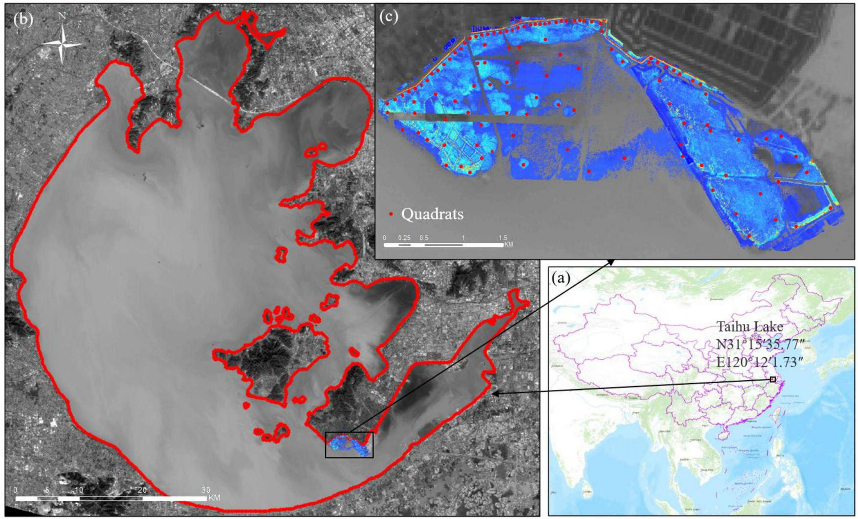
(a) Location of the study area, (b) Grayscale map of Lake Taihu using Landsat 8 OLI B4 (RED) band, showing the location of the study area, and (c) DSM map of the study area obtained from UAV data, showing sampling point distribution locations.
The East Taihu Lake is very shallow. This study covers the lakeshore zone at the mouth of East Taihu Lake Suzhou Bay, located at the southern tip of Dongshan Island (Figure 1c). This region is rich in aquatic vegetation. Field surveys indicate that the area is primarily dominated by emergent aquatic vegetation (EAV), floating-leaf aquatic vegetations (FLAV), and submerged aquatic vegetation (SAV; Table 1). It is an ideal location for developing fine-scale classification methods for plant associations.
TABLE 1
| Vegetation formation | Association and dominant species | Common names of dominant species | Abbreviation |
| EAV (emergent aquatic vegetation) | Phragmites australis | Common reed | Pa |
| Zizania latifolia | Manchurian wild rice | Zl | |
| Nelumbo nucifera | Sacred lotus | Nn | |
| FLAV (floating-leaf aquatic vegetations) | Trapa natans | Water chestnut | Tn |
| Nymphoides peltata | Yellow floating heart | Np | |
| SAV (submerged aquatic vegetation) | Not identified to species level | SAV |
Main aquatic vegetation formation, association and dominant species in the study area.
The aquatic plant associations of species composition, distribution areas, and dynamics in this region not only directly affect water quality, water supply security, and fishery production, but also play a key role in the ecological succession of the lake. Recently, many researchers have focused on aquatic plants of East Lake Taihu (Wang et al., 2022; Luo et al., 2023; Yang et al., 2023). Mapping the spatial distribution of plant associations in this lakeshore area is essential for managing the lake ecosystem.
2.2 Methods
The general workflow for this study is illustrated in Figure 2. Three tasks follow: (1) In situ quadrat investigation with UAV data acquisition and preprocessing, (2) data processing extraction of quadrat classification indicators, and (3) decision tree model and validation, generating vegetation classification maps.
FIGURE 2
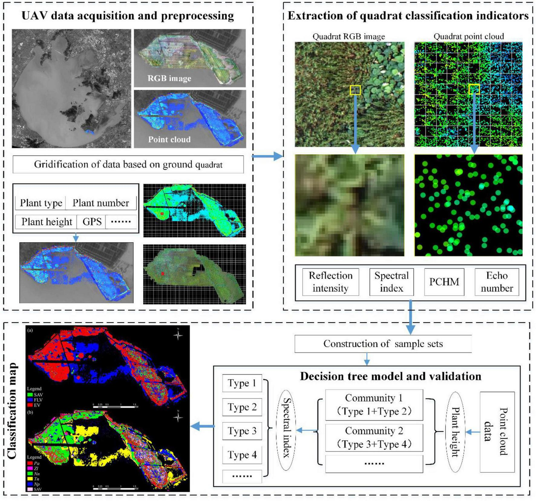
General workflow of study.
2.2.1 Data collection and processing
2.2.1.1 Field data collection and processing
Field surveys were conducted during the peak growing season of aquatic plants in 2023 from June 20 to 25 and from June 27 to 30. A total of 111 quadrats were set up in the study area (Figure 1c), each quadrat was 1 m × 1 m. For each quadrat, in situ records were kept, providing a database of plant species composition. Moreover, the plant count and height were measured for each species using a tape measure. Water depth and center coordinates of each plot were recorded concurrently; then, underwater and over water surface heights were calculated for each quadrat. All plants within the quadrat were harvested, and biomass (fresh weight) were measured separately.
2.2.1.2 Unmanned aerial vehicle (UAV) data collection and processing
The UAV data collection was synchronized with in situ plot surveys using a DJI M300 real time kinematic (RTK) drone equipped with an L1 LiDAR sensor, L1 RGB camera, and RTK system. The L1 LiDAR sensor uses the 905 nm band, with a maximum power of 60 W. The ranging accuracy (Root Mean Square, RMS 1σ) is an error of 3 cm at 100 m. The system accuracy (RMS 1σ) is as follows: the planar accuracy is an error of 10 cm at 50 m; the elevation accuracy is an error of 5 cm at 50 m. It supports a maximum of 3 echoes. The field of view (FOV) is 70.4 × 4.5° for repetitive scanning; and 70.4 × 77.2 for non-repetitive scanning. The point cloud data rate is a maximum of 240,000 points per second for a single echo; and a maximum of 480,000 points per second for multiple echoes. The L1 RGB camera has an image resolution of 20 million pixels, a focal length of 8.8 mm/24 mm (equivalent), a sensor size of 1 inch, a shutter speed of 1/2000-8 s for the mechanical shutter; and 1/8000-8 s for the electronic shutter. The ISO is 100–3200 (automatic), and 100–12800 (manual), and the aperture is f/2.8-f/11. Data was collected at an altitude of 100 m in a zigzag flight pattern, covering the entire study area. Collected data included flight path and waypoint information for aquatic vegetations and water surfaces, airborne triangulation (AT) data, RGB imagery, and point cloud scatter data.
The UAV flight control system and RTK system calculated flight trajectories, waypoint information, and AT data. Airborne triangulation is a key step in UAV photogrammetry due to its ability to utilize precise camera positioning, and record at each exposure using RTK equipment, as a crucial observational parameter in AT calculations. This approach accurately established the 3D coordinates of the camera’s phase center at each exposure, achieving high-precision geographic information acquisition for map production.
Use the L1 RGB camera on the UAV to capture RGB images, and use the L1 LiDAR sensor on the UAV to record real-time point clouds. After that, use the airborne triangulation (AT) data to geo-reference both these RGB images and the point cloud data. The flight speed is set at 10 m/s, the flight altitude is 100 m, the pitch angle of the gimbal is −60°, the scanning angle range is from −35° to 35°, the laser side overlap rate was 10%, the visible - light side overlap rate was 70%, the number of echoes was 3, the sampling frequency was 160 Hz, and the resolution of the orthophoto was 2.73 cm/pixel. The point cloud resolution was 119 points/m2. Colorized point cloud data were generated with RGB information at a resolution of 0.1 m and a horizontal accuracy of 0.1 m, as well as a vertical accuracy of 0.05 m. AT data was used to geo-reference point cloud data and produce RGB orthophotos, point cloud scatter data, and true-color point cloud data.
The purpose of surveying ground quadrats is to validate UAV point cloud data (Figure 3). This requires performing spatial alignment between field data and UAV data, ensuring each quadrat corresponds precisely to a grid cell in the point cloud dataset. This alignment enables the validation of point cloud accuracy and the classification precision of vegetation or terrain samples within the designated quadrats.
FIGURE 3
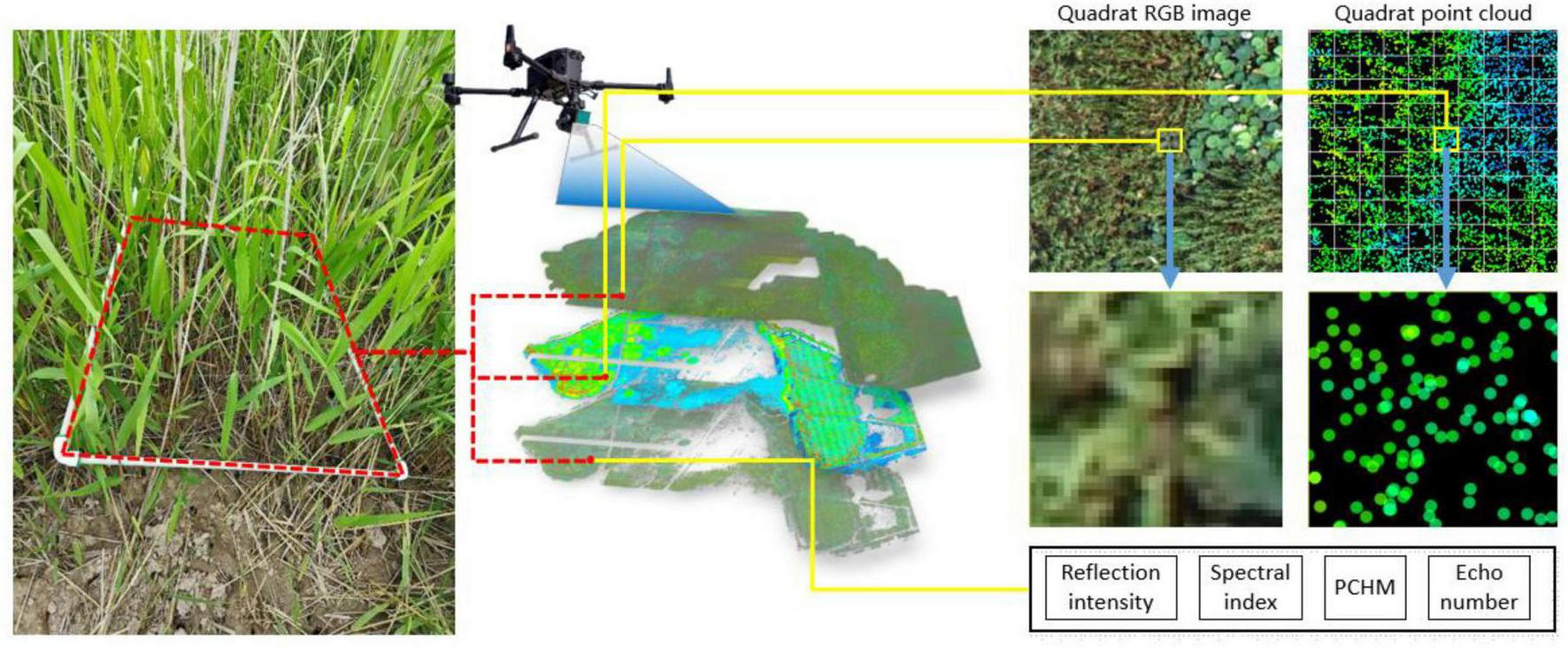
The correspondence between quadrats and point cloud.
2.2.2 Construction of the PCHM model
The aquatic plant association height was calculated using a canopy height model (CHM), which integrates a digital surface model (DSM) and digital elevation model (DEM; Bendig et al., 2014). DSMs and DEMs are typically represented by either regular rectangular grids or irregular triangulated networks. When point cloud data is converted into grids or triangulated networks, the process can be highly labor-intensive and may reduce data integrity and accuracy. In this study, we developed a direct point-based approach for constructing a point cloud digital surface model (PDSM) and a point cloud digital elevation model (PDEM) to calculate aquatic plant association height. This point cloud canopy height model (PCHM) represents the aquatic plant association canopy height (Equation 1) and was evaluated using the R2 and RMSE between estimated and measured canopy heights.
The specific workflow includes initial preprocessing of point cloud point cloud data, using DJI Terra v.4.0.10 software. Preprocessing removes noise points with abnormal heights and automatically classifies ground and water surface points, which are used to construct the PDEM (Figure 4a). Remaining points are categorized as vegetation points and used to create the PDSM (Figure 4d). The XY coordinates of the PCHM match those of the PDSM (Figures 4b, c). In the PCHM, canopy height is determined on a point-by-point basis. For each PDSM point, the nearest PDEM point is identified based on XY coordinates, and the difference between their heights (Z-axis values) represents the canopy height. Each point in the PCHM contains RGB information, spatial position, and canopy height for the aquatic plant association.
FIGURE 4
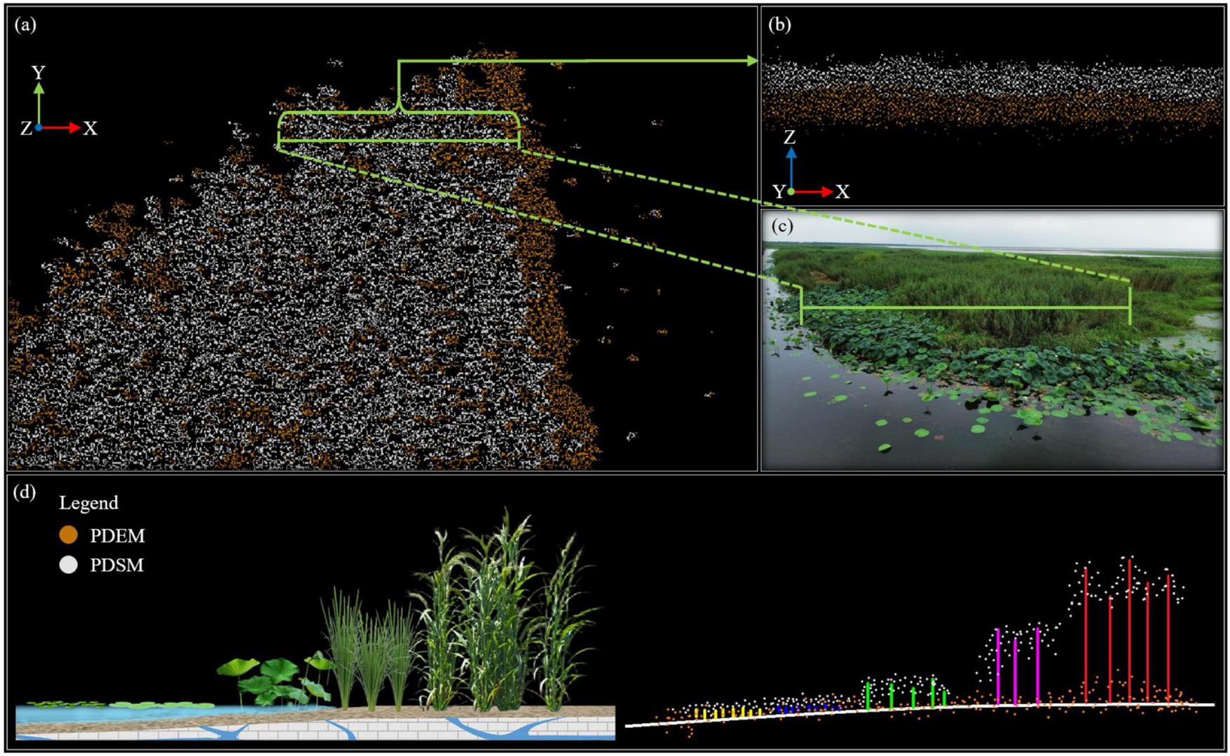
Preprocessed PDEM and PDSM. (a) PDEM and PDSM from a top-down view, (b) PDEM and PDSM in cross-sectional view (horizontal perspective), (c) actual photograph of point location, and (d) profile illustration of the wetland vegetation point cloud data acquired by UAV LiDAR.
2.2.3 Establishment of VDVI index for aquatic plant associations in littoral zone
This study employed the visible light spectrum to construct a vegetation index (VI) for aquatic vegetation by calculating the visible-band difference vegetation index (VDVI; Equation 2) based on RGB data from scatter points (Wang et al., 2015). The DJI M300 RTK UAV used in this study is only equipped with an RGB camera (without a multispectral sensor), and VDVI is calculated based on RGB bands, which can be directly extracted from existing data; in contrast, NDVI requires near-infrared band data, which cannot be obtained with the existing equipment. Statistical analysis of the VDVI across representative sample points of dominant species in the study area revealed that while VDVI can distinguish certain aquatic plant associations, it faces significant limitations for fine-scale classification of aquatic plant associations. This challenge is primarily because the VDVI index, built from optical bands, captures only differences in vegetation canopy characteristics and lacks the capacity to discern vegetation’s vertical structural information. However, in the FLAV, because the vegetation canopy is flush with the water surface, there is no necessity for information on the vertical structure of vegetation; instead, only VDVI is employed for differentiation.
Moreover, our analysis found instances where aquatic plant associations with similar VDVI values had significant height differences, illustrating the phenomenon of similar height, different spectrum; similar spectrum, different height. This observation indicates that, when paired with the PCHM, the VDVI can support precise mapping and classification of aquatic plant associations (Figure 5).
FIGURE 5
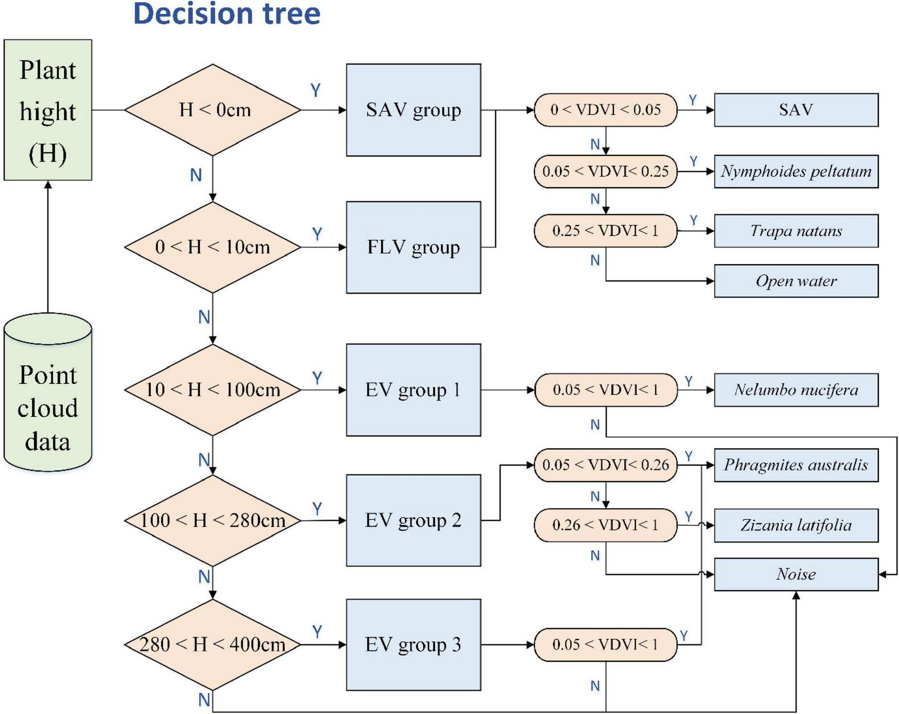
Decision tree model flow chart.
The calculation formula of the Visible-Band Difference Vegetation Index (VDVI) is expressed as follows:
with a value range of –1 ≤ VDVI ≤ 1, where G denotes the visible green band, R represents the visible red band, and B stands for the visible blue band.
To mitigate the influence of outliers and leverage the inherent separation between groups, a non-parametric threshold selection method was employed, structured as follows:
(1) Data Trimming
For each group, the top 5% and bottom 5% of values were truncated, retaining the central 90% of the data distribution (i.e., the 5th to 95th percentiles). This step reduces noise from extreme values while preserving the core distribution characteristics.
(2) Non-Overlapping Interval Validation
The trimmed ranges were defined as (Equation 3) for group Gi. A separation condition was evaluated: (or vice versa), the threshold is calculated as T (Equation 4). This ensures a clear boundary between groups.
Trimming Process: For a dataset i, the retained interval after trimming is:
Threshold Definition: If groups G1 and G2 satisfy Q95(G1) < Q5(G2), the threshold T is:
In the formulas (3) and (4) for non-overlapping interval validation above, i represents the index of the dataset, x represents an individual data point within the dataset, X represents the dataset. Q represents a percentile where Q5 specifically stands for the 5th percentile (a value below which 5% of the data in the dataset lies) and Q95 represents the 95th percentile (a value below which 95% of the data in the dataset lies), G represents a group, and T represents the classification threshold used to clearly distinguish between two groups when the separation condition is satisfied.
(3) Iterative Robustness Adjustment
If overlap persisted after initial trimming, the truncation proportion was incrementally increased (e.g., 10%, 15%) until the separation condition was satisfied. This iterative approach balances minimal data loss with reliable threshold identification.
2.2.4 Fine-scale classification method for aquatic plant associations in the littoral zone using PCHM and VDVI
The classification of aquatic plant associations was performed based on the point cloud canopy height model (PCHM) and the visible-band difference vegetation index (VDVI). A decision tree model was employed, using a two-layer conditional filter to classify aquatic plant associations (Figure 5). In wetland ecosystems, there were significant differences between emergent and floating-leaf aquatic vegetations associations in their heights relative to the water surface (Table 2). The water level fluctuation can affect the distribution of aquatic vegetation, especially during the germination and seedling stages where water level fluctuations have a significant impact on the growth and distribution of aquatic plants. This article only focuses on the remote sensing classification of typical aquatic vegetation during the vigorous growth period. Based on our field observation results and other research finding (Tippery et al., 2021), we conclude that even when these floating leaf plants are in vigorous growth or lifted by wind and waves, they will not rise more than 20 cm above the water surface. The heights of emergent aquatic vegetation associations usually were about tens of centimeters or more, for instance, generally Ass. Phragmites australis reached 200–350 cm; Ass. Zizania latifolia 100–200 cm, and Ass. Nelumbo nucifera just fewer than 100 cm over water surface. In contrast, the leaves of floating-leaf aquatic vegetations associations floated on the water surface unless dense growth, with their flowers emerging above the water surface. When the density was too high or they were lifted by wind-wave forces, the leaves could rise above water surface. However, generally neither the flowers nor the leaves would be more than 20 cm over water surface. For example, Ass Nymphoides peltata generally do not exceed 10 cm over water surface.
TABLE 2
| Dominant species | Abbreviation | Average canopy height over water surface |
| Phragmites australis | Pa | 2.70 m |
| Zizania latifolia | Zl | 1.86 m |
| Nelumbo nucifera | Nn | 0.40 m |
| Trapa natans | Tn | 0 m |
| Nymphoides peltata | Np | 0 m |
Measured average canopy height of aquatic plant associations over the water surface.
The initial step to classifying plant associations into three major groups begins with height data obtained from LiDAR: These vegetation formations are submerged aquatic vegetation (SAV) and floating-leaf aquatic vegetations differentiation among associations within the same formation. We identified VDVI value differences between associations of distinct species. For example, both Zizania latifolia and Phragmites australis belong to emergent aquatic vegetation formations and have similar average heights (1.86 m and 2.70 m, respectively). However, their VDVI ranges are markedly different, averaging 0.3924 for Zizania latifolia and 0.1938 for Phragmites australis.
Following this approach, we trained VDVI thresholds for each association sample and constructed a two-tier decision tree classification model. This model was then applied to the study area to achieve fine-scale remote sensing classification and mapping of the aquatic plant associations.
Importantly, both VDVI values and plant elevation of aquatic vegetation exhibit temporal variability. The sampling period chosen in this study corresponds to the peak growing season for most aquatic species, ensuring that the VDVI and elevation thresholds derived herein can be applied to inter-annual vegetation classification during this specific seasonal window.
3 Results
3.1 Validation of calculation results of point cloud canopy height model (PCHM)
Canopy height is a key parameter for identifying aquatic plant associations. In this study, the point cloud canopy height model (PCHM) was developed for calculating the canopy heights of plant associations (see Section “2.2.2 Construction of the PCHM model”). While using UVAs to obtain the point cloud data of typical aquatic plant associations in the study area, we conducted on-site measurements of the canopy heights of three types of emergent aquatic plant associations in 111 quadrats. We compared the model calculated results and the measured heights to verify the accuracy of the model. The validation indicated that the Ass. Phragmites australis had the greatest canopy height and the highest PCHM accuracy (R2 = 0.97, RMSE = 0.0999 m). The Ass. Zizania latifolia ranked second in canopy height and PCHM accuracy (R2 = 0.96, RMSE = 0.0942 m). The Ass. Nelumbo nucifera had the lowest canopy height and the lowest PCHM accuracy (R2 = 0.88, RMSE = 0.0620 m) (Figure 6).
FIGURE 6
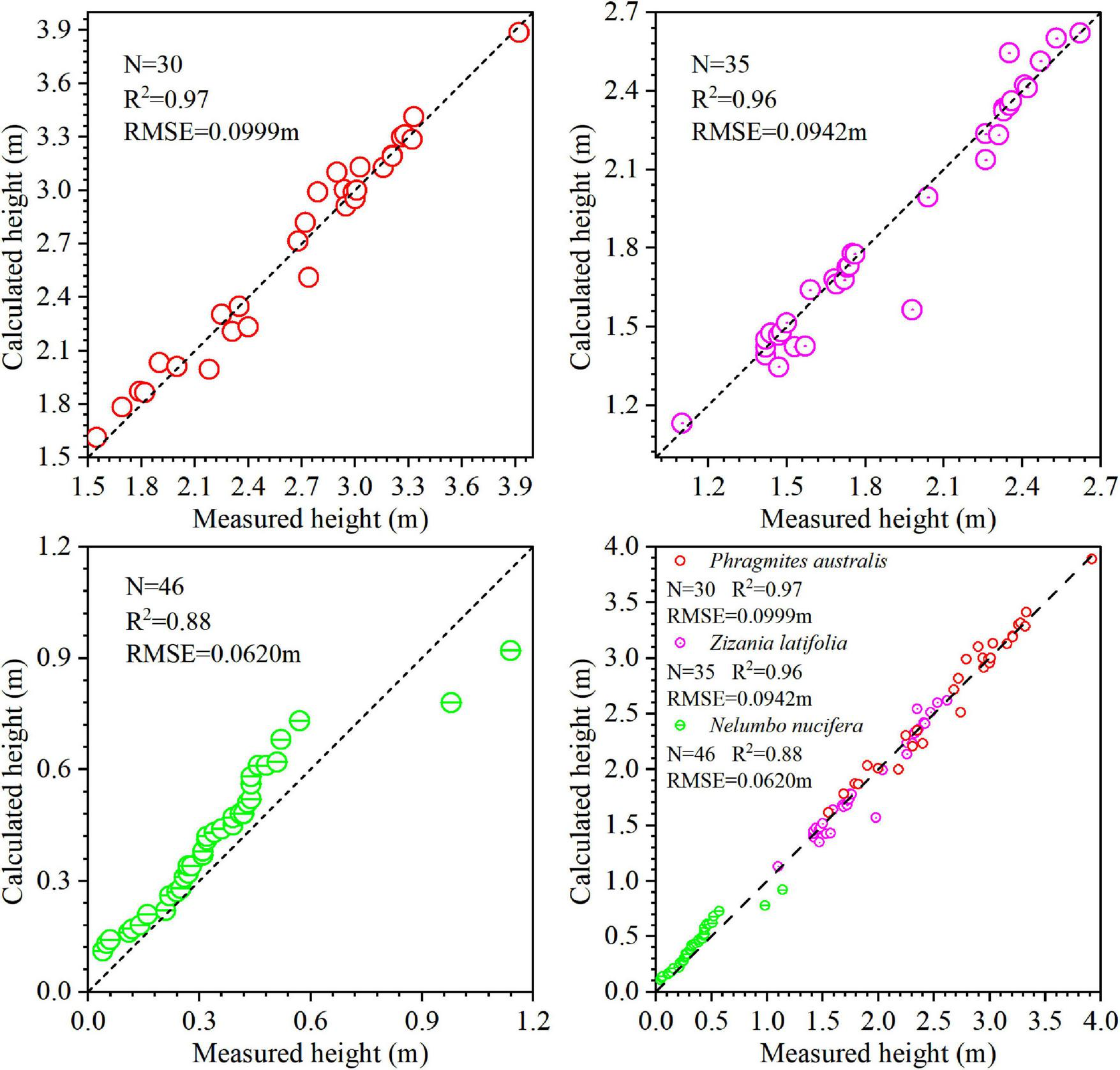
Scatter Plot of field-measurements vs. LiDAR-derived sample heights. Red points represent Ass. Phragmites australis, green points represent Ass. Zizania latifolia, and purplish red points represent Ass. Nelumbo nucifera.
However, it is difficult to distinguish between the floating-leaf aquatic vegetations associations, submerged vegetation, and the water surface using this model. Therefore, it is necessary to comprehensively utilize other information and further discuss methods for more accurate classification.
3.2 Classification of aquatic plant associations using a decision tree model
The optical information of plant associations is a key parameter for identifying aquatic plant associations. In this study, the VDVI was used to obtain the optical information of different associations. Through the location information in the ground quadrats, we accurately knew the associations represented by the point clouds within some of the grids. By calculating the RGB features in the point clouds corresponding to different associations, we found that there were significant differences in the VDVI indices of different associations. According to the calculation results of the VDVI model (Figure 7), the VDVI value of the Ass. Zizania latifolia is the highest (with an average value of 0.3565), followed by that of the Ass. Trapa natans (with an average value of 0.3291), and there is a certain overlap between them. The average VDVI values of Ass. Phragmites australis, Ass. Nelumbo nucifera, and Ass. Nymphoides peltata are 0.1607, 0.1713, and 0.1245, respectively, and there is also a certain overlap among them. The average VDVI value of the submerged vegetation is the lowest, only 0.0272, and the average VDVI value of the open water surface is negative. Therefore, it is very difficult to classify aquatic plant associations using only the VDVI index.
FIGURE 7
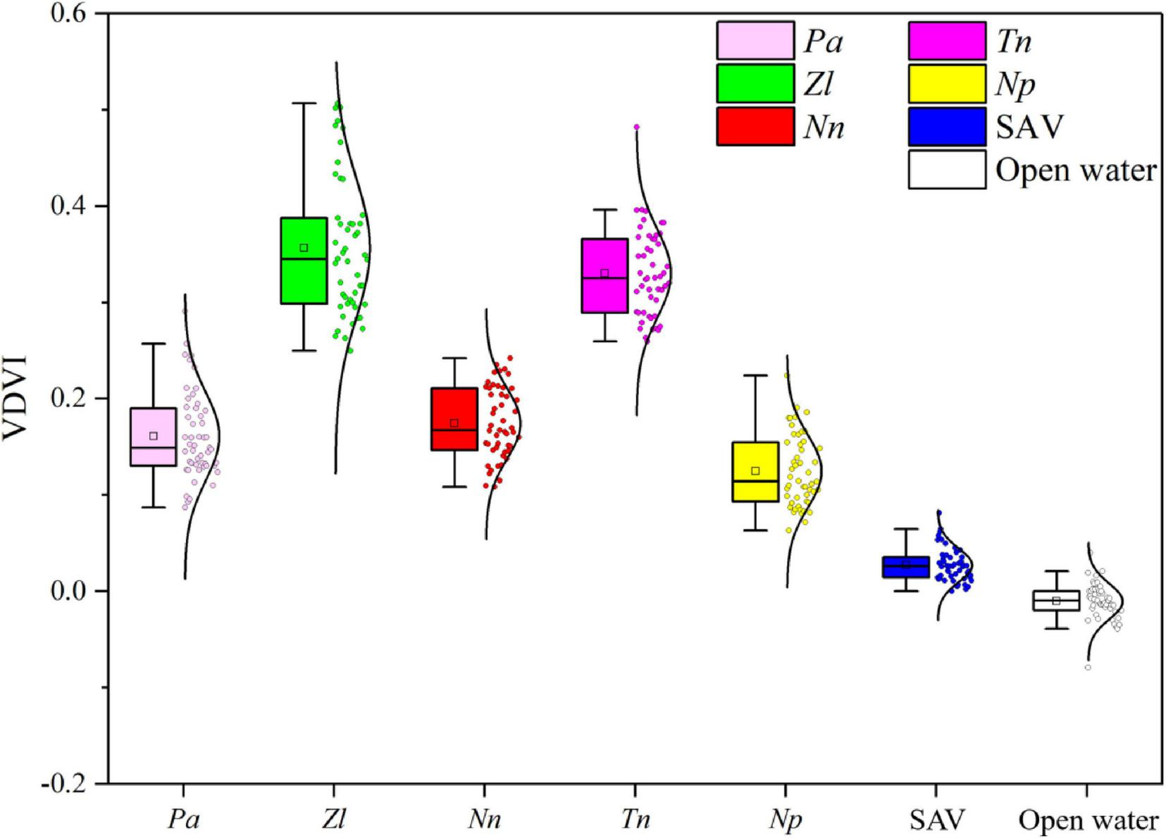
Visible-band difference vegetation index (VDVI) values of dominant aquatic plant associations in the study area.
The decision tree model was created and used to classify aquatic plant associations. A 0.1 m resolution distribution map of typical vegetation formations and aquatic plant associations in the study area was produced (Figures 8a, b).
FIGURE 8
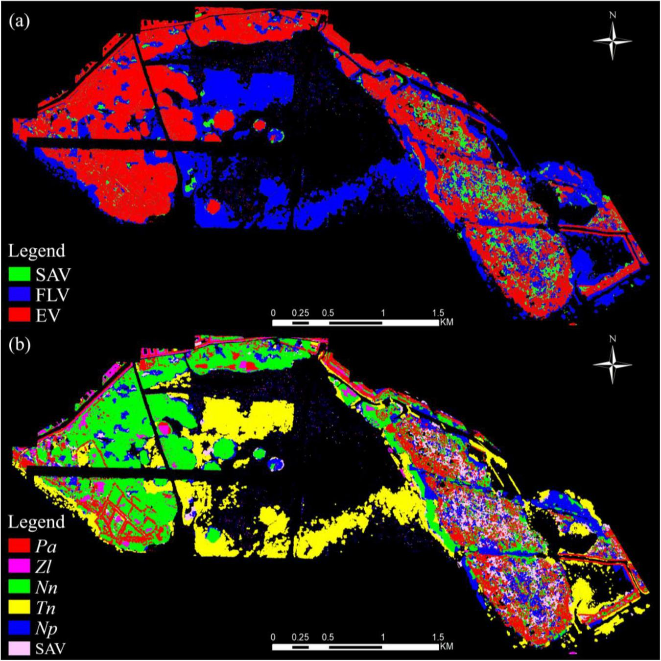
(a) Distribution of typical aquatic vegetation formations in the study area and (b) distribution of aquatic plant associations in the study area.
The total study area spans approximately 8.87 km2. The distribution areas of the following associations are: the floating-leaf aquatic vegetations (FLAV) covers 1.78 km2, including the water chestnut association covers 1.22 km2; yellow floating heart association covers 0.56 km2, and emergent aquatic vegetation (EAV) covers 3.81 km2, as well as the sacred lotus association covers 1.47 km2. The common reed association covers 0.77 km2, and the Manchurian wild rice association covers 1.57 km2. The submerged aquatic vegetation (SAV) covers about 0.26 km2.
The study area was formerly occupied by enclosing nets and man-made fishponds designed to create fish farms. In order to restore the lake ecosystem and improve the water quality, since 2019, all the enclosing nets and fishponds have been completely removed, and the project of returning fishing areas to the lake has been implemented. However, the embankments of some fishponds are still underwater. The common reed association predominantly distributes in stripped along the lakeshore, or in grid-like embankments around former fishponds. Many large patches of the sacred lotus association can be found in the central area of former fishponds. Generally, the common reed grows in shallow areas, often on the embankments of former fish ponds or lakeshore, and the sacred lotus grows in the deeper area such as the center area of fishpond. The Manchurian wild rice association distributes in the deeper water area below the distribution belt of common reed. The associated floating-leaf aquatic vegetations, such as water chestnut association and the yellow floating heart association are distributed in patches in the deepest areas of the former fishpond. This interpreted distribution of aquatic plant associations is based on the decision tree model, which aligns well with the actual vegetation distribution and topographic features in the study area.
3.3 Accuracy verification of aquatic plant association classifications
A total of 3,000 random samples were manually selected from RGB images, and classification accuracy was validated using an error matrix. The results indicated an overall classification accuracy of 87.93% and a kappa coefficient of 0.855 (Figure 9). Classification accuracy varied across vegetation formations, with mapping accuracy ranging from 75% to 95.52% and user accuracy from 79.8% to 97.4%. Higher canopy of aquatic plant associations demonstrated higher classification accuracy, with the emergent association Ass. Phragmites australis achieving the highest classification accuracy at 97.40%, followed by Ass. Zizania latifolia at 93.80%, and Ass. Nelumbo nucifera at 91.20%. Floating-leaf associations exhibited lower accuracy, Ass. Nymphoides peltata at 80.20%, Ass. Trapa natans recording the lowest classification accuracy at 79.80% (Table 3).
FIGURE 9
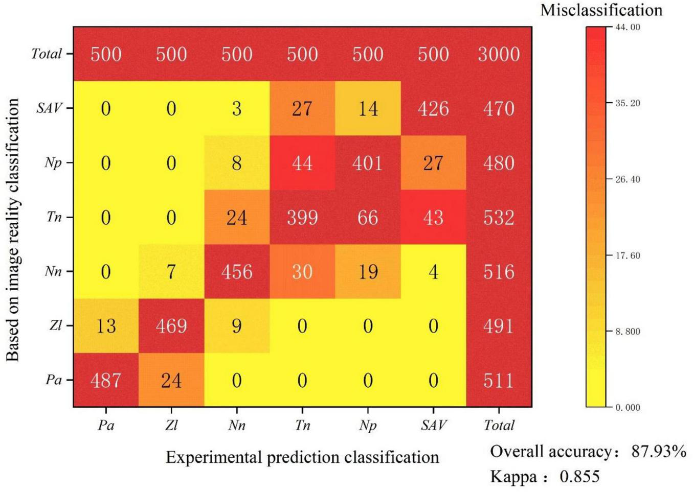
Confusion matrix. The y-axis represents true classification based on RGB images, and the x-axis represents the predicted classifications. Red cells along the diagonal indicate the number of correctly classified pixels, with each category’s total quantity evaluated shown at the top and totals of real classifications on the right. Other cells represent misclassified samples: The gradient from yellow to red signifies increasing classification error, with yellow indicating minimal error and red indicating maximal error.
TABLE 3
| Association | Mapping accuracy | Omission | User accuracy | Commission |
| Pa | 95.30% | 4.70% | 97.40% | 2.60% |
| Zl | 95.52% | 4.48% | 93.80% | 6.20% |
| Nn | 88.37% | 11.63% | 91.20% | 8.80% |
| Tn | 75.00% | 25.00% | 79.80% | 20.20% |
| Np | 83.54% | 16.46% | 80.20% | 19.80% |
| SAV | 90.64% | 9.36% | 85.20% | 14.80% |
Confusion in matrix statistical accuracy.
4 Discussion
4.1 Advantages of UAV LiDAR point cloud data in wetland vegetation applications
The complex and inaccessible environment of the lakeshore zone makes it challenging to obtain extensive, high-resolution maps of aquatic plant associations. Traditional studies, while often relying on satellite data, typically differentiate only between general vegetation formations and water bodies; therefore, traditional studies are limited in achieving fine-scale classifications of aquatic plant associations. This approach also faces challenges in distinguishing between aquatic vegetation and algal blooms in eutrophic waters. The spatial heterogeneity of lakeshore aquatic vegetation, especially in enclosed bays, often contains many small patches of aquatic plant associations that exhibit spectral similarity. Constrained by the spatial and spectral resolution of satellite data, even high-resolution satellite imagery can miss capturing the differences in these patches.
In this study, we utilized a combination of UAV LiDAR and RGB imagery to overcome these limitations. By capturing high-resolution elevation and color information from point cloud data and RGB imagery, we developed a precise classification method. Grid processing of UAV point cloud data enabled alignment with ground survey plots, enhancing classification model reliability and accuracy, allowing fine-scale classification of vegetation from formation level to association levels. The high accuracy of this method effectively replaces traditional field sampling and can cover sample areas on a spatial scale, covering several square kilometers.
Moreover, UAV-based LiDAR provides high-precision point cloud data, making it possible to improve classification accuracy at a lower cost. Previous studies have used LiDAR to identify specific plant species, and our method also demonstrated a high precision for reed (Phragmites australis) identification, which is consistent with previous findings (Onojeghuo et al., 2010; Gilmore et al., 2012; Onojeghuo and Blackburn, 2011). Compared with traditional satellite imagery-based methods, LiDAR offers significant advantages due to its capability to capture both horizontal and vertical structural information (Stratoulias et al., 2015; Sun et al., 2023). This study extends the application of LiDAR to complex environments containing multiple species, maintaining accuracy in species identification despite high biodiversity.
4.2 Accuracy of the decision tree model based on the PCHM model and VDVI index
Given the characteristics of aquatic plant associations, their point cloud data exhibit significant spatial heterogeneity. For different plant associations, distinct features can be observed in both height and VDVI index values when applying specific thresholds. Therefore, the selection of classification algorithms should prioritize models with strong interpretability (Tian et al., 2024). This interpretability is critical for vegetation classification studies using point cloud data, as understanding the underlying logic and rationale behind classification is essential in wetland ecological research. Such transparency allows researchers to clearly visualize the role of each feature in the classification process and how combinations of different features influence final results, thereby facilitating verification of corresponding plant parameters.
Moreover, point cloud datasets typically possess characteristics of large volume and high dimensionality, necessitating substantial computational resources and time for processing and analysis. Decision tree algorithms demonstrate superior computational efficiency in handling such large-scale datasets. Unlike black-box models such as neural networks and deep learning, whose internal decision-making processes are inherently opaque, decision trees provide explicit classification rules that can be easily interpreted. Additionally, training neural networks requires extensive amounts of labeled data, which is often impractical to obtain for accurately annotated point cloud datasets (Yao et al., 2022). Neural networks also suffer from challenges related to complex parameter tuning and optimization, increasing the risk of overfitting and compromising model generalization capabilities. The primary objective of this study is to establish a highly reliable and accurate method for generating interpretable large-scale training datasets.
The constructed point cloud canopy height model (PCHM) demonstrates satisfactory accuracy across three plant associations, with the Ass. Phragmites australis achieving the highest precision (R2 = 0.97 and RMSE = 0.0999 m), while the Ass. Nelumbo nucifera has the lowest canopy height, which exhibits the lowest precision (R2 = 0.88 and RMSE = 0.0620 m, as shown in Figure 7). Research on vegetation height often employs CHM models, typically using UAV (Khosravipour et al., 2015; Hao et al., 2021; Sumnall et al., 2017) or satellite LiDAR data (Tamiminia et al., 2024; Torresani et al., 2023), primarily to study forest trees. While satellite data information struggles to achieve high precision for low-lying vegetation, some satellite datasets, such as ICESat-2 ATL08 and GEDI L2A products, monitor vegetation height. ICESat-2 ATL08 samples were found along a track at approximately 0.7 m intervals with areas measured between 11 and 12 m. Each group was spaced 90 m apart along 3.3 km tracks. GEDI L2A’s ground footprint diameter measured 25 m, spaced 60 m along the track (Liu et al., 2021). Although this data lacks the resolution needed to accurately assess ground vegetation height, it is widely used for identifying tall forest trees. However, relying solely on satellite data in complex aquatic habitats for low-lying aquatic vegetation is insufficient. In contrast, the UAV LiDAR data employed in this study achieved 0.1 m precision in canopy height measurements, allowing for accurate fine-grained classifications of small community patches. Our method has been compared to existing studies and exhibits superior accuracy relative to the precision requirements of each respective research objective (Table 4). This method effectively replaces traditional manual field sampling, extending sample plot dimensions to the square-kilometer scale and providing essential ground sampling data for satellite remote sensing to perform quantitative, detailed aquatic community classifications. The same approach can be used to complete different tasks: (1) to conduct future quantitative vegetation parameter retrieval, (2) to address current challenges in obtaining ground sample data for quantitative modeling of aquatic vegetation parameters and (3) to expand the scope of aquatic vegetation remote sensing.
TABLE 4
| CHM method | Data source of CHM | Model accuracy (highest) |
| Khosravipour et al., 2015 | Helicopter LiDAR | R2 = 0.54, RMSE = 0.32 m |
| Hao et al., 2021 | UAV RGB | R2 = 0.87, RMSE = 0.24 m |
| Tamiminia et al., 2024 | GEDI 2A, Sentinel-2 MSI, Sentinel-1 SAR | R2 = 0.74, RMSE = 4.40 m |
| Torresani et al., 2023 | GEDI 2A | R2 = 0.73 |
| Sumnall et al., 2017 | UAV Lidar | R2 = 0.87, RMSE = 2.10 m |
| Our methods | UAV Lidar | R2 = 0.97, RMSE = 0.0999 m |
Authors’ new canopy height mode (CHM) accuracy compared with existing research.
The overall trend in wetland plant classification accuracy shows that taller vegetation tends to achieve higher classification precision, with elevation accuracy differences directly impacting final classification results. LiDAR systems may encounter challenges when scanning low-growing vegetation, often misclassifying plant structures with water surfaces or soil, resulting in significant noise points that distort actual elevation measurements. For FLAV Ass. Nymphoides peltate and Ass. Trapa natans, their identical elevation values (as they float on the water surface) necessitate exclusive reliance on VDVI thresholds for differentiation. This results in inherently lower classification accuracy compared to EAV, which benefit from additional height-based discrimination. The main reason for the low classification accuracy of Nymphoides peltate and Trapa natans is sole reliance on VDVI, and the causes also include: first, the similar growth morphology of Nymphoides peltate and Trapa natans (both are floating-leaf plants with similar leaf sizes, approximately 5–10 cm), resulting in small differences in canopy structure information obtained by LiDAR; second, the mosaic growth of Nymphoides peltate and Trapa natans in some areas of East Taihu Lake (patch size < 5 m), leading to a high proportion of mixed pixels (about 20%), which further intensifies spectral confusion; third, water background interference (superposition of reflectance spectra of floating-leaf vegetation and water surface), making it impossible for VDVI to effectively distinguish the boundary between vegetation and background.
Secondly, among EAV, Ass. Nelumbo nucifera exhibits the lowest classification accuracy due to its high variability in growth heights, ranging from floating leaf structures at water level to significantly elevated stems above the surface. In contrast, Ass. Zizania latifolia and Ass. Phragmites australis demonstrate more homogeneous height distributions, which likely contributes to their significantly higher classification accuracies compared to Ass. Nelumbo nucifera. Beyond the height-related traits that support their classification accuracy, these two EAV associations also present distinct spatial distribution patterns and associated ecological impacts—factors that further highlight the practical value of their precise identification and mapping. Ass. Phragmites australis is mainly distributed in the upper part of the lakeshore zone, specifically the near-shore area, and grows densely in strips; this growth habit allows it to easily form a single dominant community, thereby occupying the ecological niches of other coexisting species. To address the potential ecological competition caused by its overexpansion, the “moderate mowing” strategy is recommended: this approach involves mowing the above-ground part of the plants every autumn while retaining their root systems, which helps control the rate of its spread without disrupting the basic ecological function of the association. Ass. Zizania latifolia, by comparison, is distributed in the lower part of the lakeshore zone, namely the deeper water area, and typically grows in patches around the embankments of former fishponds. A key ecological concern with this association is that the decomposition of its residual biomass tends to cause water quality deterioration. To mitigate this issue and restore the surrounding habitat, the “seasonal cleaning + habitat restoration” strategy is proposed: this strategy includes removing aged plant residues in spring and simultaneously introducing submerged vegetation such as Potamogeton crispus to construct a composite vegetation system, which in turn helps improve the overall water quality of the area.
4.3 The ecological significance of aquatic vegetation classification
Accurate classification of aquatic vegetation is essential for ecosystem monitoring and management. The composition and density of aquatic vegetations significantly impact ecosystem structure and function. Emergent and floating-leaf vegetations near shorelines can trap sediments and pollutants, support biodiversity, and contribute biomass. However, excessive growth and biomass accumulation of emergent aquatic vegetations can adversely affect water quality, potentially leading to Brownification water (Li, 1997; Wang et al., 2022) and lake bogginess (Zhang et al., 1999). Aquatic vegetation types are considered key components of aquatic ecosystems, especially in shallow lakes when submerged vegetations maintain a clear water state (i.e., the macrophyte-dominated state), which sustains the clear water phase. Aquatic vegetation largely determines the composition of other hydrobionts and the course of various processes. The emergent and floating-leaf vegetation define the functioning of the lake ecosystem and its resilience.
It is crucial to have precise and timely information on the distribution of aquatic vegetation in both lakeshore zones and lake areas. The findings of this study offer scientific support for planning and managing ecological reserves, assessing lake resources, and monitoring environmental conditions, as well as aiding in ecological conservation and sustainable resource utilization. Additionally, incorporating high-resolution multispectral satellite data synchronized with UAV data can further enhance the accuracy and scope of aquatic vegetation classification.
5 Conclusion
This study established an accurate classification method for aquatic plant associations by combining UAV LiDAR point cloud data and RGB imagery (0.1 m spatial resolution). Using PCHM and a decision tree model, the study achieved precise mapping from a general vegetation formation down to a specific association level, resulting in a high-resolution distribution map of lakeshore aquatic vegetation.
The classification accuracy for emergent associations in East Lake Taihu ranged from 75% to 95.52% with a user accuracy between 79.8% and 97.4% and a kappa coefficient of 0.855. Among emergent associations, Ass. Phragmites australis achieved the highest accuracy at 97.40%, followed by Ass. Zizania latifolia at 93.80% and Ass. Nelumbo nucifera at 91.20%. Floating-leaf associations showed lower classification accuracy, Ass. Nymphoides peltata achieved accuracy at 80.20%, and Ass. Trapa natans achieved accuracy at 79.80%.
Unmanned aerial vehicle LiDAR technology enables precise recognition of aquatic vegetation formations down to the association level, with promising applications based on a large-scale identification using optical and SAR satellites. This method offers a reliable alternative to traditional field sampling and can support quantitative inversion of structural parameters like biomass, paving the way for advancements in aquatic vegetation remote sensing.
Statements
Data availability statement
The datasets presented in this study can be found in online repositories. The names of the repository/repositories and accession number(s) can be found in the article/supplementary material.
Author contributions
YW: Investigation, Formal analysis, Validation, Writing – review & editing, Writing – original draft, Data curation, Resources, Supervision, Conceptualization, Visualization, Methodology, Software, Project administration. JG: Writing – review & editing, Supervision, Conceptualization, Funding acquisition. QG: Writing – original draft, Investigation. WW: Investigation, Writing – original draft. GL: Investigation, Writing – original draft. JL: Writing – review & editing, Conceptualization, Funding acquisition, Supervision.
Funding
The author(s) declare financial support was received for the research and/or publication of this article. The study was supported by the National Natural Science Foundation of China (42271377 and 41971043) and Open Project Funding of Key Laboratory of Intelligent Health Perception and Ecological Restoration of Rivers and Lakes, Ministry of Education, Hubei University of Technology (HGKFZ09).
Acknowledgments
We would like to thank the reviewers for their thoughtful comments and suggestions on the manuscript.
Conflict of interest
The authors declare that the research was conducted in the absence of any commercial or financial relationships that could be construed as a potential conflict of interest.
Generative AI statement
The authors declare that no Generative AI was used in the creation of this manuscript.
Any alternative text (alt text) provided alongside figures in this article has been generated by Frontiers with the support of artificial intelligence and reasonable efforts have been made to ensure accuracy, including review by the authors wherever possible. If you identify any issues, please contact us.
Publisher’s note
All claims expressed in this article are solely those of the authors and do not necessarily represent those of their affiliated organizations, or those of the publisher, the editors and the reviewers. Any product that may be evaluated in this article, or claim that may be made by its manufacturer, is not guaranteed or endorsed by the publisher.
References
1
Ban S. Toda T. Koyama M. Ishikawa K. Kohzu A. Imai A. (2019). Modern lake ecosystem management by sustainable harvesting and effective utilization of aquatic macrophytes.Limnology2093–100. 10.1007/s10201-018-0557-z
2
Bendig J. Bolten A. Bennertz S. Broscheit J. Eichfuss S. Bareth G. (2014). Estimating biomass of barley using crop surface models (CSMs) derived from UAV based RGB imaging.Remote Sens.610395–10412. 10.3390/rs61110395
3
Cao Y. (2007). Study on impact factor and technique of vegetation restoration for flood beaches wetlands along Yangtze River.PhD thesis, Nanjing Normal University: Nanjing.
4
Cheng F. Y. Van Meter K. J. Byrnes D. K. Basu N. B. (2020). Maximizing US nitrate removal through wetland protection and restoration.Nature588625–630. 10.1038/s41586-020-03042-5
5
Delle Grazie F. M. Gill L. W. (2022). Review of the ecosystem services of temperate wetlands and their valuation tools.Water14:1345. 10.3390/w14091345
6
Engelhardt K. Ritchie M. (2001). Effects of macrophyte species richness on wetland ecosystem functioning and services.Nature411687–689. 10.1038/35079573
7
Gilmore M. S. Wilson E. H. Barrett N. Civco D. L. Prisloe S. Hurd J. D. et al (2012). Integrating multi-temporal spectral and structural information to map wetland vegetation in a lower Connecticut River tidal marsh.Remote Sens. Environ.1124048–4060. 10.1016/j.rse.2008.05.020
8
Hao Z. B. Lin L. L. Post C. J. Mikhailova E. A. Li M. H. Chen Y. et al (2021). Automated tree-crown and height detection in a young forest plantation using mask region-based convolutional neural network (Mask R-CNN).ISPRS J. Photogrammetry Remote Sens.178112–123. 10.1016/j.isprsjprs.2021.06.003
9
Hong M. G. Nam B. E. Kim J. G. (2021). Phragmites australis makes valuable floating mat biotopes under oligotrophic conditions.Landscape Ecol. Eng.17109–118. 10.1007/s11355-020-00440-9
10
Hu T. Sun X. Su Y. Guan H. Sun Q. Kelly M. et al (2021). Development and performance evaluation of a very low-cost UAV-Lidar system for forestry applications.Remote Sens.13:77. 10.3390/rs13010077
11
Jennings M. D. Faber-Langendoen D. Loucks O. L. Peet R. K. Roberts D. (2009). Standards for associations and alliances of the U.S. National vegetation classification.Ecol. Monographs79173–199. 10.1890/07-1804.1
12
Khanna S. Santos M. J. Ustin S. L. Haverkamp P. J. (2011). An integrated approach to a biophysiologically based classification of floating aquatic macrophytes.Int. J. Remote Sens.321067–1094. 10.1080/01431160903505328
13
Khosravipour A. Skidmore A. K. Wang T. J. Isenburg M. Khoshelham K. (2015). Effect of slope on treetop detection using a LiDAR canopy height model.ISPRS J. Photogrammetry Remote Sens.10444–52. 10.1016/j.isprsjprs.2015.02.013
14
Kornijów R. Kowalewski G. Sugier P. Kaczorowska A. Gąsiorowski M. Woszczyk M. (2016). Towards a more precisely defined macrophyte-dominated regime: The recent history of a shallow lake in Eastern Poland.Hydrobiologia77245–62. 10.1007/s10750-015-2624-3
15
Landucci F. Šumberová K. Tichý L. Hennekens S. Aunina L. Biţă-Nicolae C. et al (2020). Classification of the European marsh vegetation (Phragmito-Magnocaricetea) to the association level.Appl. Veg. Sci.23297–316. 10.1111/avsc.12484
16
Lawniczak-Malinska A. E. Achtenberg K. (2018). On the use of macrophytes to maintain functionality of overgrown lowland lakes.Ecol. Eng.11352–60. 10.1016/j.ecoleng.2018.02.003
17
Li W. C. (1997). Yellow water in east taihu lake caused by Zizania latifolia and its prevention.J. Lake Sci.9364–368. 10.18307/1997.0412
18
Li Z. F. Zhang X. K. Wan A. Wang H. L. Xie J. (2018). Effects of water depth and substrate type on rhizome bud sprouting and growth in Zizania latifolia.Wetlands Ecol. Manag.26277–284. 10.1007/s11273-017-9572-9
19
Liu A. B. Cheng X. Chen Z. Q. (2021). Performance evaluation of GEDI and ICESat-2 laser altimeter data for terrain and canopy height retrievals.Remote Sens. Environ.264:112571. 10.1016/j.rse.2021.112571
20
Luo J. H. Ni G. Zhang Y. L. Wang K. Shen M. Cao Z. G. et al (2023). A new technique for quantifying algal bloom, floating/emergent and submerged vegetation in eutrophic shallow lakes using Landsat imagery.Remote Sens. Environ.287:113480. 10.1016/j.rse.2023.113480
21
Luo J. H. Yang J. Z. C. Duan H. T. Lu L. R. Sun Z. Xin Y. H. (2022). Research progress of aquatic vegetation remote sensing in shallow lakes.Natl. Remote Sens. Bull.2668–76. 10.11834/jrs.20221208
22
Onojeghuo A. O. Blackburn G. A. (2011). Optimising the use of hyperspectral and LiDAR data for mapping reedbed habitats.Remote Sens. Environ.1152025–2034. 10.1016/j.rse.2011.04.004
23
Onojeghuo A. O. Blackburn G. A. Latif Z. A. (2010). “Characterising reedbed habitat quality using Leaf-off LiDAR data,” in Proceedings of the 2010 6th international colloquium on signal processing & its applications, (Malaca: IEEE).
24
Puletti N. Guasti M. Innocenti S. Cesaretti L. Chiavetta U. A. (2024). Semi-Automatic approach for tree crown competition indices assessment from UAV LiDAR.Remote Sens.16:2576. 10.3390/rs16142576
25
Ronowski R. Chmara R. Szmeja J. (2023). Structural and functional changes in macrophyte species composition in softwater lakes after 60 years of land use.Aquatic Sci.85:104. 10.1007/s00027-023-00999-z
26
Sayer C. D. Burgess A. Kari K. Davidson T. A. Peglar S. Yang H. et al (2010). Long-term dynamics of submerged macrophytes and algae in a small and shallow, eutrophic lake: Implications for the stability of macrophyte-dominance.Freshwater Biol.55565–583. 10.1111/j.1365-2427.2009.02353.x
27
Shin S. Mohibbullah M. Kim K. Y. Hong E. J. Choi J. S. Ku S. K. (2024). Therapeutic potential of water chestnut fruit extract (Trapa bicornis) against ovariectomy-induced climacteric symptoms in mice.Appl. Sci.14:7464. 10.3390/app14177464
28
Stratoulias D. Balzter H. Sykioti O. Zlinszky A. Tóth V. R. (2015). Evaluating Sentinel-2 for lakeshore habitat mapping based on airborne hyperspectral data.Sensors1522956–22969. 10.3390/s150922956
29
Sumnall M. Thomas R. F. Randolph H. W. Valerie A. T. (2017). Mapping the height and spatial cover of features beneath the forest canopy at small-scales using airborne scanning discrete return Lidar.ISPRS J. Photogrammetry Remote Sens.133186–200. 10.1016/j.isprsjprs.2017.10.002
30
Sun C. Li J. L. Liu Y. C. Zhao S. H. Zheng J. H. (2023). Tracking annual changes in the distribution and composition of saltmarsh vegetation on the Jiangsu coast of China using Landsat time series–based phenological parameters.Remote Sens. Environ.284:113370. 10.1016/j.rse.2022.113370
31
Tamiminia H. Salehi B. Mahdianpari M. Goulden T. (2024). State-wide forest canopy height and aboveground biomass map for New York with 10 m resolution, integrating GEDI, Sentinel-1, and Sentinel-2 data.Ecol. Inform.79:102404. 10.1016/j.ecoinf.2023.102404
32
Temmink R. J. M. Lamers L. P. M. Angelini C. Bouma T. J. Fritz C. van de Koppel J. (2022). Recovering wetland biogeomorphic feedbacks to restore the world’s biotic carbon hotspots.Science376:eabn1479. 10.1126/science.abn1479
33
Thomaz S. M. (2023). Ecosystem services provided by freshwater macrophytes.Hydrobiologia8502757–2777. 10.1007/s10750-021-04739-y
34
Tian Y. Zhang Q. Tao J. Zhang Y. Lin J. Bai X. et al (2024). Use of interpretable machine learning for understanding ecosystem service trade-offs and their driving mechanisms in karst peak-cluster depression basin, China.Ecol. Indicat.166:112474. 10.1016/j.ecolind.2024.112474
35
Tippery N. P. Pawinski K. C. Jeninga A. J. (2021). Taxonomic evaluation of Nymphoides (Menyanthaceae) in eastern Asia.Blumea66249–262. 10.3767/blumea.2021.66.03.08
36
Torresani M. Rocchini D. Alberti A. Moudrý V. Heym M. Thouverai E. et al (2023). LiDAR GEDI derived tree canopy height heterogeneity reveals patterns of biodiversity in forest ecosystems.Ecol. Inform.76:102082. 10.1016/j.ecoinf.2023.102082
37
Wang X. Q. Wang M. M. Wang S. Q. Wu Y. D. (2015). Extraction of vegetation information from visible unmanned aerial vehicle images (in Chinese with English abstract).Trans. Chin. Soc. Agricultural Eng.31152–159. 10.3969/j.issn.1002-6819.2015.05.022
38
Wang Y. W. Xu J. Li J. Y. Liu J. (2022). changes of aquatic vegetation and water quality after removal of pen aquaculture in lake East Taihu.J. Ecol. Rural Environ.38104–111. 10.19741/j.issn.1673-4831.2020.0986
39
Yang C. T. Shen X. B. Wu J. B. Shi X. Y. Cui Z. J. Tao Y. W. et al (2023). Driving forces and recovery potential of the macrophyte decline in East Taihu Lake.J. Environ. Manag.342:118154. 10.1016/j.jenvman.2023.118154
40
Yao J. Sun S. Zhai H. Feger K. H. Zhang L. Tang X. et al (2022). Dynamic monitoring of the largest reservoir in North China based on multi-source satellite remote sensing from 2013 to 2022: Water area, water level, water storage and water quality.Ecol. Indicat.144:109470. 10.1016/j.ecolind.2022.109470
41
Yu H. Lv T. Wang H. Y. Li D. X. Wang L. G. Fang S. F. et al (2022). A preliminary scheme for an aquatic vegetation classification in China (in Chinese).Sci. Sinica Vitae521335–1355. 10.1360/ssv-2022-0060
42
Zhang S. Z. Wang G. X. Pu P. M. Chigira T. (1999). Succession of hydrophytic vegetation and swampy tendency in the East Taihu Lake.J. Plant Resources Environ.81–6.
43
Zhu Q. Zheng R. W. Zeng L. Q. Li C. H. Ye C. (2024). Control of overgrowth of Potamogeton crispus in shallow lakes by light shading and artificial introductions.Environ. Technol. Innovat.35:103641. 10.1016/j.eti.2024.103641
Summary
Keywords
aquatic vegetation, association classification, LiDAR point cloud, unmanned aerial vehicle (UAV), remote sensing, lakeshore wetland, East Lake Taihu
Citation
Wang Y, Gao J, Guo Q, Wang W, Liu G and Luo J (2025) UAV-based LiDAR and optical imagery fusion for fine-scale classification of aquatic plant associations in lakeshore wetlands. Front. For. Glob. Change 8:1698796. doi: 10.3389/ffgc.2025.1698796
Received
04 September 2025
Accepted
20 October 2025
Published
05 November 2025
Volume
8 - 2025
Edited by
Mingming Jia, Chinese Academy of Sciences (CAS), China
Reviewed by
Chao Chen, Suzhou University of Science and Technology, China
Zhaohui Xue, Hohai University, China
Updates
Copyright
© 2025 Wang, Gao, Guo, Wang, Liu and Luo.
This is an open-access article distributed under the terms of the Creative Commons Attribution License (CC BY). The use, distribution or reproduction in other forums is permitted, provided the original author(s) and the copyright owner(s) are credited and that the original publication in this journal is cited, in accordance with accepted academic practice. No use, distribution or reproduction is permitted which does not comply with these terms.
*Correspondence: Jian Gao, jgao13@hotmail.comJuhua Luo, jhluo@niglas.ac.cn
Disclaimer
All claims expressed in this article are solely those of the authors and do not necessarily represent those of their affiliated organizations, or those of the publisher, the editors and the reviewers. Any product that may be evaluated in this article or claim that may be made by its manufacturer is not guaranteed or endorsed by the publisher.