Improving agricultural commodity allocation and market regulation: a novel hybrid model based on dual decomposition and enhanced BiLSTM for price prediction

As an essential part of daily life, the drastic fluctuations in agricultural commodity prices significantly impact producers’ motivation and consumers’ quality of life, further exacerbating market uncertainty and unsustainability. The ability to scientifically and effectively predict agricultural commodity prices is of great significance for the rational deployment of market mechanisms, the timely adjustment of supply chains, and the promotion of food policy adjustments. This paper proposes a sustainable hybrid model SV-PSO-BiLSTM which integrates Seasonal-Trend decomposition procedure based on Loess (STL), Variational Mode Decomposition (VMD), Particle Swarm Optimization (PSO), and Bidirectional Long Short-Term Memory (BiLSTM) neural networks. This innovative approach first performs seasonal decomposition of the original data using the STL method, then applies the VMD method for double decomposition of the residual components, reconstructs the data based on sample entropy, and finally predicts agricultural commodity market prices using the BiLSTM network model optimized by the PSO algorithm. This paper investigates the market price dynamics of four agricultural commodities (chili, garlic, ginger, and pork) and one agricultural financial derivative (soybean futures). The experimental results indicate that the proposed SV-PSO-BiLSTM hybrid model achieves average values of 0.2241 for root mean square error (RMSE), 0.1665 for mean absolute error (MAE), 0.0207 for mean absolute percentage error (MAPE), and 0.9851 for the coefficient of determination (R²). These results surpass those of other comparative models, demonstrating stronger generalization, reliability, and stability. The research findings can provide effective guidance for the reasonable regulation of agricultural commodity market prices and further promote the healthy and sustainable development of the agricultural commodity industry.

1 Introduction

Agricultural commodities are an important component of diets, and their prices are directly related to farmers’ income and people’s happiness index. In a country like China, which possesses a vast agricultural product market, the frequent fluctuations in agricultural commodity prices directly affect the efficiency of resource allocation. When the price of a particular agricultural commodity rises, farmers typically increase the production of that product while neglecting other equally important crops. This can lead to an imbalance between supply and demand, resulting in shortages of certain agricultural commodities in the future. Conversely, when prices fall, farmers’ motivation may wane, potentially leading to idle land and reduced production, further exacerbating issues of market supply insufficiency (Du, 2020). Such short-term production adjustments not only influence farmers’ income but also have far-reaching impacts on the overall market’s resource allocation and regulatory mechanisms. In addition, high prices often stimulate overproduction, leading to environmental pressures such as soil degradation and excessive use of water resources (Jia et al., 2022). Over time, this can easily trigger market instability and social dissatisfaction. Therefore, accurately predicting agricultural commodity prices has become a significant concern across various sectors of society, which is essential for responding to market fluctuations, enhancing people’s happiness index, promoting the sustainable development of the agricultural commodity industry, and fostering the coordinated development of regional economies and the environment (Li et al., 2023).

Traditional agricultural product price prediction methods include regression analysis, time series prediction, gray model, etc. (Jadhav et al., 2017; Wu et al., 2016; Feng et al., 2012; Ma et al., 2022), which are based on solid theoretical foundation and have strong interpretability. However, these methods are generally suitable for cases where variables are independent, data is normally distributed, and linear or simple nonlinear relationships exist. For example, Wang and Wang (2016) applied GM (1,1) model to make short-term prediction of vegetable yield in China. Ge and Wu (2020) used a multiple linear regression model to predict corn price, but the model lacked a comprehensive examination of the complex internal facto00rs driving price changes, and its performance was still not satisfactory.

In recent years, algorithms based on machine learning have become a new way to solve the problem of price prediction. Typical machine learning models include reverse support vector machine (SVM), propagation neural network (BP), convolutional neural network (CNN), and long short-term memory network (LSTM), etc. (Haider et al., 2019, Kurumatani, 2020, Adisa et al., 2019, Chen et al., 2024). Wang (2023) used radial basis function (RBF) neural network to predict garlic price and proved the superiority of the proposed model. Fan et al. (2021) realized the prediction of soybean futures price through LSTM neural network model. Jiang et al. (2021) used BiLSTM, a two-way LSTM network, to forecast cotton prices and achieved good results. Li et al. (2013) used CNN to predict the weekly egg price in China, and the results show that the model has high nonlinear fitting ability and good performance.

Although machine learning methods show good learning ability, a single model is usually easily affected by random factors. Properly combining multiple prediction methods to form a hybrid prediction model can make full use of sample data information and thus improve the accuracy of prediction (Sun et al., 2023). Guo et al. (2022) realized the accurate prediction of corn price by constructing AttLSTM-ARMIA-BP model. Cheung et al. (2023) proposed a clustering 3D-CNN model to predict future crop prices, which has achieved good results. Ling et al. (2019) developed a GM-VAR hybrid model to predict the prices of various livestock products, and their prediction results were superior to a single prediction model.

In addition, in order to reduce the influence of characteristics such as noise, trend and period inherent in complex data, domestic and foreign scholars combine decomposition techniques with prediction models (Fang et al., 2021, Fan et al., 2023, Tang et al., 2023). The advantage of the “decomposition-combination” prediction model is that it can utilize information at different scales, thus improving the accuracy and robustness of the prediction. Selecting the appropriate data decomposition method is the key to the model. At present, the commonly used decomposition methods include seasonal decomposition (Tatarintsev et al., 2021, Liu et al., 2020), variational mode decomposition (Liao, 2024, Wu et al., 2024), wavelet decomposition (Cao and He, 2015), and empirical mode decomposition (Lai et al., 2024), etc. For example, Yin et al. (2020) proposed the STL-AttLSTM model to accurately predict the prices of five crops: cabbage, radish, onion, pepper and garlic. Hu and Jiang (2023) adopted the hybrid model of VMD-BO-BiLSTM to achieve accurate prediction of pork price. Xiong et al. (2018) proposed an extreme value learning machine method based on the decomposition of seasonal trends based on STL, and predicted the prices of Chinese cabbage, chili, cucumber, green bean and tomato. Zhang B. et al. (2024) combined the integrated ensemble empirical mode decomposition (EEMD) method with the gated recurrent units (GRU) to establish an EEMD-GRU model for predicting Chinese corn, cotton and soybean futures, which has obvious advantages in prediction accuracy.

From previous research, it can be seen that although there have been significant advancements in agricultural product price prediction technologies, there are still many shortcomings. For example, there is an insufficiency of effective prediction methods, issues with modal aliasing of the residual components after decomposition, excessively high time complexity of the models, and numerous parameters in neural network models that are difficult to adjust. All of these factors can lead to insufficient predictive accuracy.

In view of the above problems, the main contributions of this paper are as follows:

1. This article proposes an innovative STL-VMD dual decomposition method, which is applied for the first time in the field of agricultural commodity price prediction. This approach effectively addresses the issue of mode mixing in the high-volatility residual components.

2. The proposed methodology implements entropy-guided K-means clustering for residual modal component reconstruction, achieving dual enhancement in both prediction accuracy and computational efficiency through spatiotemporal complexity optimization.

3. The STL-VMD dual decomposition method, combined with the PSO optimization algorithm and the BiLSTM neural network, establishes the SV-PSO-BiLSTM ensemble model for agricultural commodity price prediction, effectively enhancing the model’s flexibility and accuracy.

4. This study selects four agricultural commodities: chili, ginger, garlic, and pork, along with soybean futures as a financial derivatives indicator. Through predictive modeling and comparative experiments, we validated the model’s effectiveness and stability in both physical agricultural products and financial instruments.

2 Materials and methods

2.1 Data

This study selects the weekly average national wholesale prices of four agricultural commodities: chili, ginger, garlic, and pork (CNY/kg), along with the closing prices of soybean futures(CNY/ton) as an agricultural financial derivative as sample data. The time spans for the data are: chili and ginger (January 6, 2006 – February 23, 2024), garlic (January 4, 2008 – December 29, 2023), pork (November 1, 2010 – July 22, 2024), and soybean futures (January 5, 2015 – October 21, 2024). To facilitate analysis, 70% of the sample data is used as a training dataset, with the remaining 30% serving as a testing dataset. To ensure experimental accuracy, the data employed in this study is sourced from the Bric Agricultural Data Terminal, which aggregates information from various statistical websites, including the China Rural Statistical Yearbook, the National Agricultural Product Business Information Public Service Platform, and the China Agricultural Product Price Survey Database. Relevant statistical information is presented in Table 1.

Table 1

Table 1. Statistical characteristics of agricultural commodity price series: descriptive analysis of chili, ginger, garlic, pork, and soybean futures markets (2006–2024).

2.2 Methods

Agricultural commodity prices exhibit significant fluctuations over time, and the data encompass intricate information such as seasonality, long-term memory, and heteroskedasticity, which may lead to reduced prediction accuracy. This paper proposes a deep learning model named SV-PSO-BiLSTM for predicting agricultural commodity price trends. This model integrates STL-VMD dual feature extraction, K-means sample entropy feature fusion, and a BiLSTM prediction architecture optimized by PSO. The SV-PSO-BiLSTM model effectively extracts features from time series data, enhances feature representation capabilities, simplifies model complexity, and improves both computational efficiency and predictive performance. The overall framework of the model is illustrated in Figure 1.

1. The first step involves performing feature extraction on the original agricultural commodity price series using the STL algorithm, aiming to capture significant seasonal and trend features.

2. The second step entails applying the VMD algorithm to the residual components resulting from the STL feature extraction, thereby further decomposing the mode-mixed residuals into n Intrinsic Mode Functions (IMFs).

3. In the third step, the sample entropy values of the n IMFs are calculated. Subsequently, the K-means algorithm is used for feature fusion, leading to the formation of three new K-IMF components.

4. The fourth step employs BiLSTM networks as the prediction model. Specifically, the trend, seasonality, and the three K-IMF components are input into their corresponding models for forecasting. Following this, the PSO algorithm is applied to optimize the hyperparameters of the BiLSTM model.

5. Lastly, in the fifth step, the predicted results from each BiLSTM model are aggregated to obtain the final prediction value. Additionally, the effectiveness of the model is validated using multiple evaluation metrics.

Figure 1

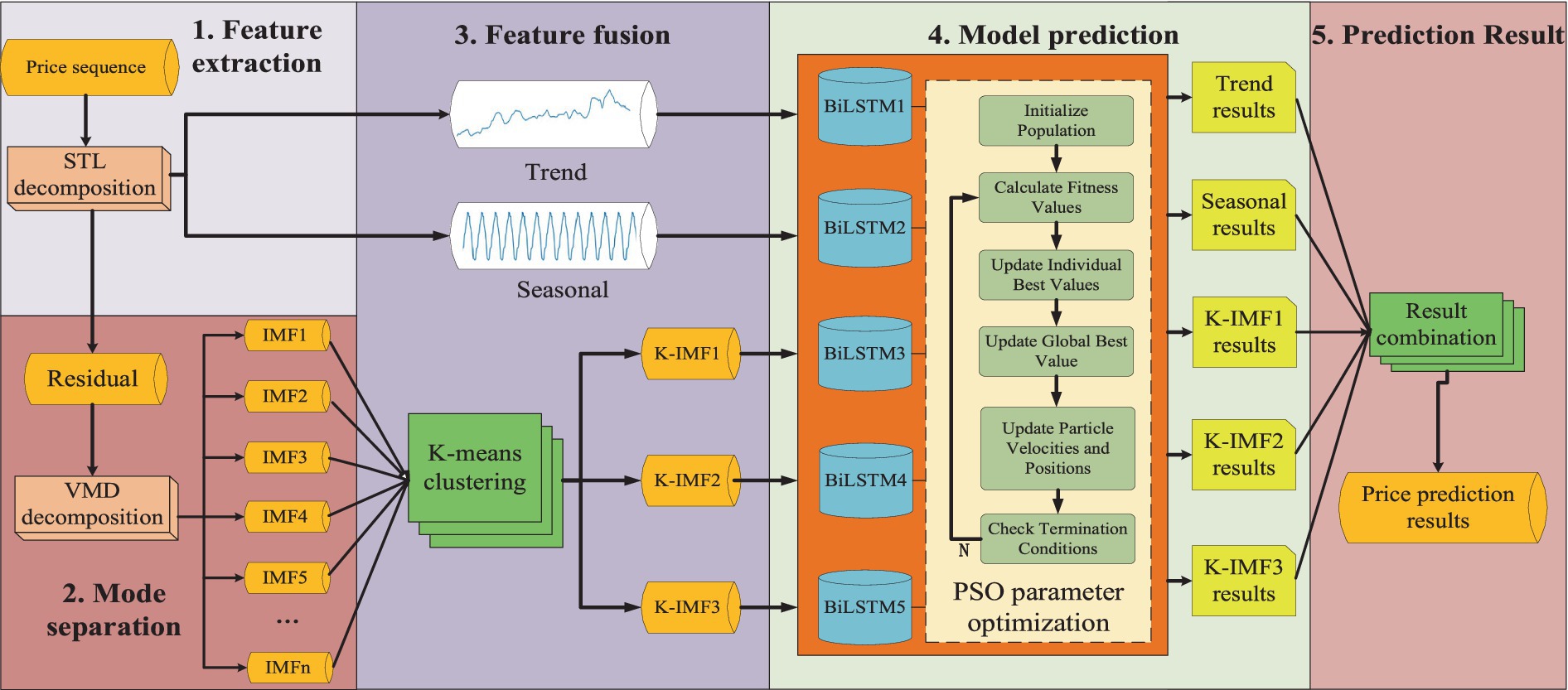
Figure 1. The SV-PSO-BiLSTM framework: a multi-stage hybrid model integrating STL-VMD dual decomposition, entropy-driven feature fusion, and PSO-optimized BiLSTM networks for agricultural commodity price prediction.

2.2.1 STL feature extraction

Agricultural commodity prices exhibit fluctuating patterns with complex nonlinear characteristics over time. Given their notable seasonal features, this paper introduces the STL algorithm to decompose agricultural commodity prices into three sub-components: trend, seasonality, and residual. STL is a typical time series decomposition method that employs robust locally weighted regression as a smoothing technique. It utilizes the Locally Weighted Scatterplot Smoothing(Loess) method to smooth and fit time series data, decomposing the data at a given time point $Y_t\left(t=1,2,\dots ,n\right)$ into seasonal component $S_t$ , trend component $C_t$ , and residual component $R_t$to achieve improved estimates of seasonality and trend. The decomposition expression is shown in Equation 1:

$\begin{array}{ll}{Y}_{\mathrm{t}}=S_t+C_t+Rt& (1)\end{array}$

The steps of establishing STL model are as follows:

(1) De-trend. After $i+1$iterations of the inner loop, the subsequence is obtained by subtracting the estimated trend component $C_t^i$from the initial sequence $Y$at the $i$iteration, as formulated in Equation 2.

$\begin{array}{ll}{Y}_t^{det\mathit{rend}}=Y_t+C_t^i& (2)\end{array}$

(2) Periodic subsequence smoothing. The local weighted regression is carried out for each $Y_t^{\mathrm{detrend}}$subsequence using Loess, and the preliminary seasonal component ${\tilde{S}}_t^{i+1}$is obtained.

(3) Low pass filtering of periodic subsequences. The preliminary seasonal component ${\tilde{S}}_t^{i+1}$ obtained in step 2 is processed by a low-pass filter, and then the sequence $L_t^{i+1}$is obtained by using Loess.

(4) Remove the tendency of smoothing periodic subsequences. The seasonal component can be obtained by calculating the difference between the value after low-pass filtering and the seasonal component obtained by preliminary calculation, and the seasonal component is defined in Equation 3.

$\begin{array}{ll}{S}_{\mathrm{t}}^{i+1}=S_{\mathrm{t}}^{i+1}-L_{\mathrm{t}}^{i+1}& (3)\end{array}$

(5) De-seasonal. By subtracting the seasonal component $S^{i+1}$ , the original sequence $Y$is obtained, as expressed in Equation 4.

$\begin{array}{ll}{Y}_t^{det\mathit{rend}}=Y_t-S_t^{i+1}& (4)\end{array}$

(6) Trend smoothing. By using the Loess method, the trend component $C_t^{i+1}$is obtained from the removing seasonal series.

The seasonal component $S$and the trend component $C$obtained from the internal cycle are calculated in the external cycle to obtain the residual component $R$ , as mathematically formulated in Equation 5.

$\begin{array}{ll}{R}_t=Y_{\mathrm{t}}-S_t-C_t& (5)\end{array}$

Compared to traditional seasonal decomposition methods, the STL algorithm demonstrates significant advantages in extracting trend and seasonal components. However, the residual component still exhibits complex nonlinear characteristics, which may include highly irregular fluctuations, sudden anomalies, or intricate interaction effects. These nonlinear characteristics make it challenging even for advanced neural network models to fully capture them, potentially leading to issues of overfitting or underfitting when dealing with these residuals. Consequently, the accuracy and reliability of prediction results are limited.

2.2.2 VMD double decomposition

Given the limitations of the STL algorithm, this paper introduces the VMD algorithm to perform secondary decomposition on the residual component, decomposing it into multiple intrinsic mode components that intuitively reflect its nature. The VMD algorithm is a completely non-recursive and adaptive data processing method that constructs and solves constrained variational problems to obtain intrinsic mode functions by updating the center frequencies and modal functions. It decomposes the original signal into a specific number of IMFs. The VMD method effectively handles nonlinear and non-stationary signals. The specific steps are as follows:

The variational formulation aims to decompose the original data into several modal components such that the sum of the bandwidths of each modal component is minimized.

$\begin{array}{l}min\left\{{\displaystyle \sum }_{m=1}^m\parallel \partial \left\{\left[\delta \left(t\right)+\frac{j}{\pi t}\right]\ast u_m\right\}t{e}^{-j{w}_{m}t}{\parallel }_2^2\right\},\hfill \\ s.t.{\displaystyle \sum }_m{u}_m=f\hfill \end{array}\text{ (6)}$

In Equation 6, $\delta \left(t\right)$is the Dirac function; m is the number of decomposed modes; $\ast$is the convolution operator; $w_m$is the central frequency of the m component; $u_m$is the MTH modal component. By introducing the quadratic penalty factor $\alpha$and the Lagrange multiplication operator $\lambda$ , the unconstrained variational problem is obtained

$\begin{array}{l}L\left(\left\{u_m\right\},\left\{w_m\right\},\lambda \right)=\alpha {\displaystyle \sum }_m\parallel \partial \left\{\left[\delta \left(t\right)+\frac{j}{\pi t}\right]\ast u_m\right\}t{e}^{-j{w}_{m}t}{\parallel }_2^2+\parallel \\ f\left(t\right)-{\displaystyle \sum }_m{u}_m\left(t\right){\parallel }_2^2+\lambda \left(t\right),f\left(t\right)-{\displaystyle \sum }_m{u}_m\left(t\right)\end{array}\text{ (7)}$

In Equation 7, the alternate direction multiplier iterative algorithm is used to optimize each mode component and center frequency, and the saddle point of the augmented Lagrange function is searched. $\alpha$ is a quadratic penalty factor used to reduce the influence of Gaussian noise. The solutions for $u_m$ 、 $w_m$and $\lambda$after iteration are

$\begin{array}{ll}{\widehat{u}}_m^{n+1}\left(w\right)=\frac{\widehat{f}\left(w\right)-{\displaystyle \sum }_{i<m}{\widehat{u}}_m^{n+1}\left(w\right)+\frac{{\widehat{\lambda }}^n\left(w\right)}{2}}{1+2\alpha {\left(w-w_m^n\right)}^2}& (8)\end{array}$

$\begin{array}{ll}{w}_m^{n+1}=\frac{{{\displaystyle \int }}_0^{\infty }w{\left|{\widehat{u}}_m^{n+1}\left(w\right)\right|}^{2}dw}{{{\displaystyle \int }}_0^{\infty }{\left|{\widehat{u}}_m^{n+1}\left(w\right)\right|}^{2}dw}& (9)\end{array}$

$\begin{array}{ll}{\widehat{\lambda }}^{n+1}={\widehat{\lambda }}^n\left(w\right)+\tau \left(\widehat{f}\left(w\right)-{\displaystyle \sum }_m\left|{\widehat{u}}_m^{n+1}\left(w\right)\right|\right)& (10)\end{array}$

In Equations 8–10, $\tau$is used as noise tolerance to ensure the fidelity of signal decomposition; ${\widehat{u}}_m\left(w\right)$ , $\widehat{f}\left(w\right)$and $\widehat{\lambda }\left(w\right)$ are the Fourier transforms of $u_m,w_m$and $\lambda$ , respectively.

Considering that secondary decomposition using the VMD algorithm can easily lead to issues such as an excessive number of residual mode components and over-decomposition, which may increase prediction errors, the K-means clustering algorithm is employed to reconstruct multiple residual mode components based on sample entropy values into three K-IMF components. This approach can effectively avoid prediction errors caused by over-decomposition and other issues while ensuring sufficient decomposition.

2.2.3 BiLSTM

Agricultural commodity prices often exhibit highly complex characteristics such as non-stationarity, nonlinearity, and time-varying behavior, making it difficult for traditional methods to fully capture their intricate internal logical relationships. The BiLSTM network is capable of learning temporal correlations between data and enhancing the extraction of time series features. It is widely used in the field of agricultural product price prediction. Therefore, this paper selects BiLSTM as the benchmark prediction model.

LSTM is a deep learning model commonly used to process and predict sequential data such as time series and text. Compared with the traditional RNN, LSTM effectively solves the problem of gradient disappearance and gradient explosion in the traditional RNN by introducing a gating mechanism, so that it can better capture long-term dependence. LSTM selects the input value by adjusting the input gate, deletes invalid information through the forget gate, transmits valid information to the next step, and outputs the result through the output gate.

BiLSTM learns bidirectional time series on this basis. The combination of forward running LSTM and backward running LSTM has the same gate unit as LSTM, and can train the time series forward and backward LSTM twice. The output result of BiLSTM is superposition of the two LSTM results, which further improves the integrity of feature extraction, and finally extracts the data feature $I_0$of $n\times m$dimension.

$\begin{array}{ll}{I}_0=\left(I_0^1,I_0^2,\cdots ,I_0^n\right)& (11)\end{array}$

In Equation 11, $I_0^n$represents the nth feature.

2.2.4 PSO parameter optimization

The complexity of the BiLSTM network necessitates a large number of parameters. To optimize these parameters and enhance the model’s performance, this paper introduces the PSO algorithm. The PSO algorithm is a swarm intelligence-based optimization technique inspired by the collective behavior of bird flocks searching for food. This optimization method is problem-independent and does not require gradient information of the objective function, thereby effectively avoiding local minima and efficiently searching for the global optimal solution within the search space. Each particle in the PSO algorithm possesses a unique velocity and position, where the position of each particle signifies a potential candidate solution to the optimization problem and is evaluated through a fitness function to ascertain its quality. Particles iteratively adjust their velocities and positions based on the relationships among their current positions, their personal best positions, and the global best position, driving them to converge toward the global optimal position and progressively approximating the solution target until the iteration terminates or the global optimal solution is discovered.

The mathematical calculation formula of particle velocity and position in PSO algorithm is as follows:

$\begin{array}{ll}{v}_{\mathit{id}}^{k+1}=w{v}_{\mathit{id}}^k+c_1{r}_1\left(\mathit{pbes}{t}_{\mathit{id}}^k-x_{\mathit{id}}^k\right)+c_2{r}_2\left(\mathit{gbes}{t}_{gd}^k-x_{\mathit{id}}^k\right)& (12)\end{array}$

$\begin{array}{ll}{x}_{\mathit{id}}^{k+1}=x_{\mathit{id}}^k+v_{\mathit{id}}^{k+1}& (13)\end{array}$

In Equations 12, 13, $v_{\mathit{id}}^{k+1}$and $v_{\mathit{id}}^k$are the velocity values of particles at adjacent moments respectively; $w$ is the inertia weight; $x_{\mathit{id}}^{k+1}$and $x_{\mathit{id}}^k$are the position values of particles at adjacent moments, respectively. $c_1$and $c_2$are learning factors. $r_1$ and $r_2$are random numbers ranging from 0 to 1. $\mathit{pbes}{t}_{\mathit{id}}^k$and $\mathit{gbes}{t}_{gd}^k$are the individual and global historical optimal location values at time k, respectively.

In this paper, we utilize the feature components that have undergone dual decomposition using STL-VMD and subsequent reconstruction as input variables for optimizing the hyperparameters of the BiLSTM network, specifically the number of neurons in the first and second layers, the learning rate, and the batch size. The MSE is employed as the fitness function to evaluate and iteratively update the positions of individuals and the population, progressively converging toward the optimal solution until the iteration terminates or the global optimum is identified, as detailed in Algorithm 1.

ALGORITHM 1

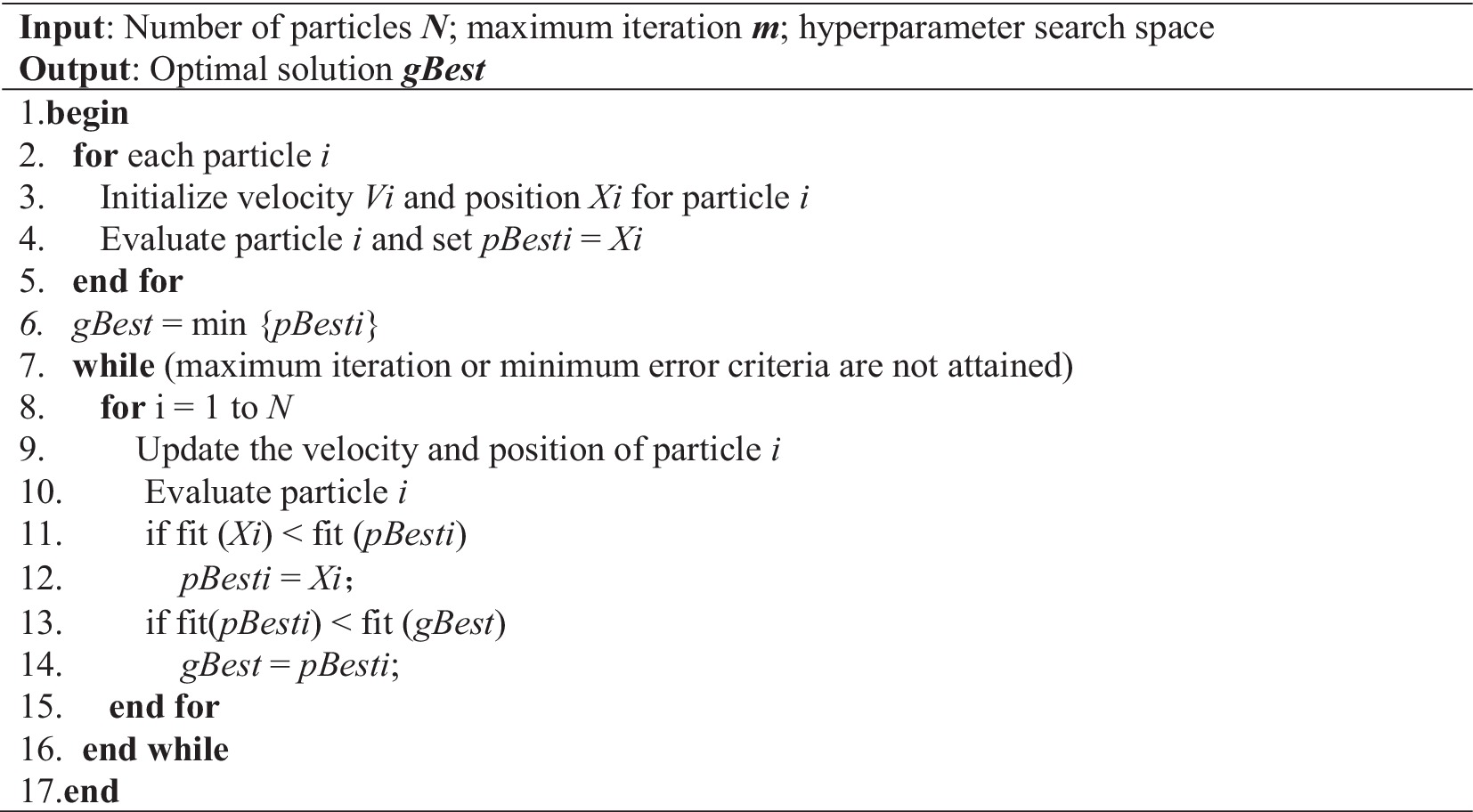
ALGORITHM 1. PSO optimization algorithm.

2.2.5 Experimental design

The core experimental design establishes a hierarchical validation framework, focusing on three highly volatile and supply-chain-sensitive agricultural commodities: chili, ginger, and garlic. A comparative experiment was conducted between our SV-PSO-BiLSTM model and nine other models, and an ablation experiment was performed specifically on our model. Additionally, to enhance the model’s generalizability and reliability, an extended adaptability experiment was carried out, incorporating pork and soybean futures to assess the model’s performance across different market structures (spot commodities and financial derivatives). Finally, a stability experiment was conducted on the core experimental subjects to further strengthen the model’s robustness and applicability.

In this experiment, 70% of the sample data is allocated to construct the training dataset, with the remaining 30% reserved for testing to assess model performance. All experimental results presented are derived from the test dataset outputs, ensuring objectivity and accuracy in evaluation. This approach strengthens the model’s generalization capability on unseen data, reinforcing the scientific validity and reliability of the research conclusions.

To evaluate the performance of different models, this study employs four widely-used error metrics as model performance evaluation criteria: RMSE, MAE, MAPE, and R², as shown in Equations 14–17. Smaller values of RMSE, MAE, and MAPE indicate higher model accuracy and reliability, while the R² value ranges between 0 and 1, with values closer to 1 signifying superior model fit.

RMSE measures the accuracy of a predictive model by calculating the square root of the average squared differences between predicted and actual values. It is particularly sensitive to outliers and reflects the predictive stability of the model.

$\begin{array}{ll}\mathit{RMSE}=\sqrt{\frac{1}{n}{\displaystyle \sum }_{i=1}^n{\left(y_i-{\widehat{y}}_i\right)}^2}& (14)\end{array}$

MAE computes the average of the absolute differences between predicted and true values to evaluate the robustness of absolute errors. It captures the overall trend of the data and assesses the model’s predictive accuracy.

$\begin{array}{ll}MAE=\frac{1}{n}{\displaystyle \sum }_{i=1}^n\mid y_i-{\widehat{y}}_i\mid & (15)\end{array}$

MAPE evaluates the accuracy of a predictive model by calculating the percentage difference between predicted and actual values. It is scale-independent, making it suitable for cross-variety prediction tasks involving datasets of varying magnitudes.

$\begin{array}{ll}\mathit{MAPE}=\frac{1}{n}{\displaystyle \sum }_{i=1}^n\mid \frac{y_i-{\widehat{y}}_i}{y_i}\mid & (16)\end{array}$

R² is a core metric for assessing the goodness-of-fit of a model. It quantifies the proportion of variance in the dependent variable explained by the independent variables, reflecting the model’s reliability and the extent to which price fluctuations can be systematically modeled.

$\begin{array}{ll}{R}^2=1-\frac{{\displaystyle \sum }_{i=1}^{\mathrm{n}}{\left(y_i-{\widehat{y}}_i\right)}^2}{{\displaystyle \sum }_{i=1}^n{\left(y_i-{\overline{y}}_i\right)}^2}& (17)\end{array}$

In Equations, $n$is the number of test sets; $y_i$is the true value of the $i$th sample point; ${\widehat{y}}_i$is the predicted value for the $i$th sample point.

This multi-metric framework ensures rigorous assessment of predictive accuracy and model interpretability through its distinct measurement dimensions and alignment with agricultural market characteristics, addressing stakeholders’ needs while preserving statistical rigor.

3 Results

3.1 STL-VMD dual decomposition and reconstruction

Step 1: STL decomposition. First, STL algorithm is used to decompose the original data set into three sub-sequences: trend component, seasonal component and residual component. According to the annual variation rule of agricultural commodity prices, the seasonal period of the STL algorithm is set to one year, and the parameter value is 50 weeks. The decomposition results are shown in Figure 2.

Figure 2

Figure 2. STL-based seasonal-trend decomposition: feature extraction results for agricultural commodity price series. (a–c) Chili, ginger, and garlic.

Step 2: VMD decomposition. Then, VMD algorithm is used to divide the residual components of high fluctuation into n effective modal components, so that the sum of decomposition bandwidths of each mode is minimized. The penalty coefficient of VMD algorithm adopts the default value 2000. The value of the tolerance is 1e-7, and the k value is determined by observing the center frequency. When the center frequency of the last component remains relatively stable, the best value of k is obtained. Through experiments, the center frequencies of each component with different k values are obtained, as shown in Table 2. For sequence 1, k = 5; for sequence 2, k = 6; for sequence 3, k = 7. The breakdown results are shown in Figures 3a–c.

Table 2

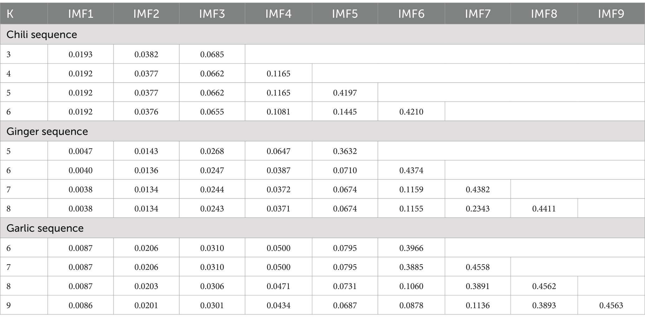
Table 2. VMD mode optimization via central frequency stability: IMF component analysis across K-values.

Figure 3

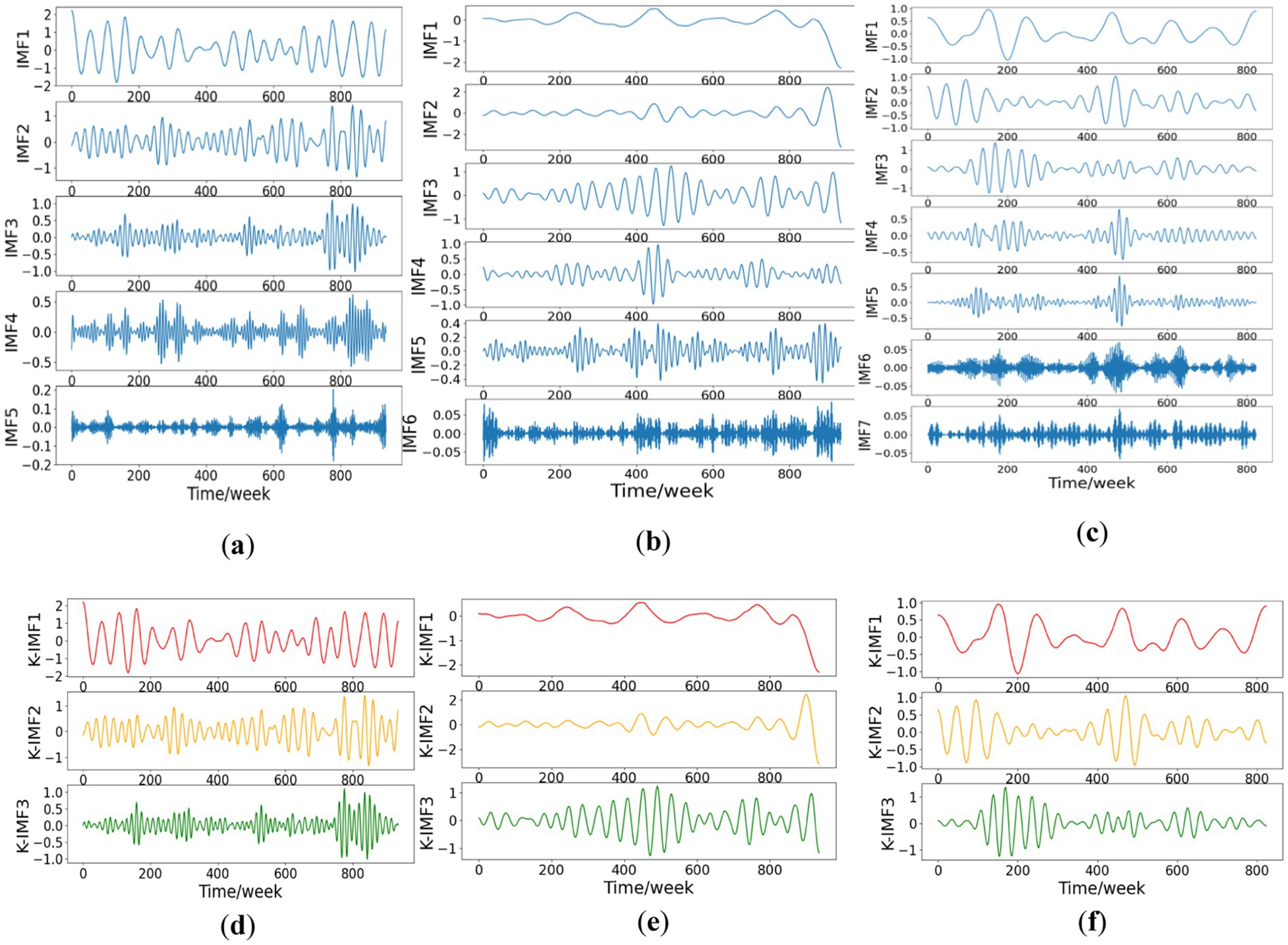
Figure 3. Hierarchical processing workflow: VMD decomposition and entropy-driven feature fusion. (a–c) Secondary VMD decomposition of STL residuals: mode separation for price series; (d–f) Entropy-K-means component reconstruction: adaptive fusion of IMFs based on sample entropy clustering.

Step 3: Entropy-K-means reconstruction. The sample entropy of n IMF components after VMD processing is calculated respectively, as shown in Equation 18. According to the sample entropy value, n IMF components are divided by K-means clustering algorithm, and three new K-IMF components are constructed. The intra-class gap is minimized and the inter-class gap is maximized, and the result is shown in Figures 3d–f.

$\begin{array}{ll}\mathit{SampEn}\left(m,r,N\right)=-ln\frac{B^{m+1}\left(r\right)}{B^m\left(r\right)}& (18)\end{array}$

In Equation 18, m is the dimension, r is the similarity tolerance, N is the finite value length, and $B^m$ is the number of patterns with length m in the sample sequence.

3.2 SV-PSO-BiLSTM model prediction

The BiLSTM model parameters and the value range of hyperparameters were initialized, and the iteration number of PSO algorithm was set to 100; Set the number of particles to 20; Keep the default values for other parameters. The search range of the number of hidden neurons in the first and second layers of BiLSTM is set to [1,100]. The learning rate ranges from [0.001, 1.000]. The batch size ranges from [16, 32]. Adam algorithm is used in the adaptive optimization phase of BiLSTM.

This paper conducts 10 experiments to compare the average results of the model. The prediction results of each component of the SV-PSO-BiLSTM model dataset are shown in Figure 4. As can be seen from the figure, the predicted values of the model closely align with the actual values.

Figure 4

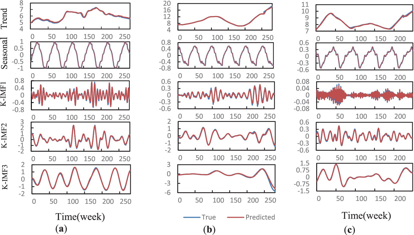
Figure 4. Multi-component prediction performance of SV-PSO-BiLSTM model: trend, seasonality, and reconstructed K-IMF fitting results. (a–c) Chili, ginger, and garlic.

3.3 Model comparison experiment

To validate the suitability of our proposed SV-PSO-BiLSTM method for agricultural commodity price prediction, we conduct comparative experiments with nine models: LSTM, Transformer, BiLSTM, BP neural network, SSA-BP, STL-BiLSTM, BO-GRU, STL-PSO-BiLSTM, and VMD-BO-BiLSTM. The first four single models are compared to identify the baseline model for constructing the hybrid model. Detailed parameter configurations for all models are provided in Supplementary Table S1.

The average evaluation metrics of the prediction results for the SV-PSO-BiLSTM model compared to other comparison models are presented in Table 3.

Table 3

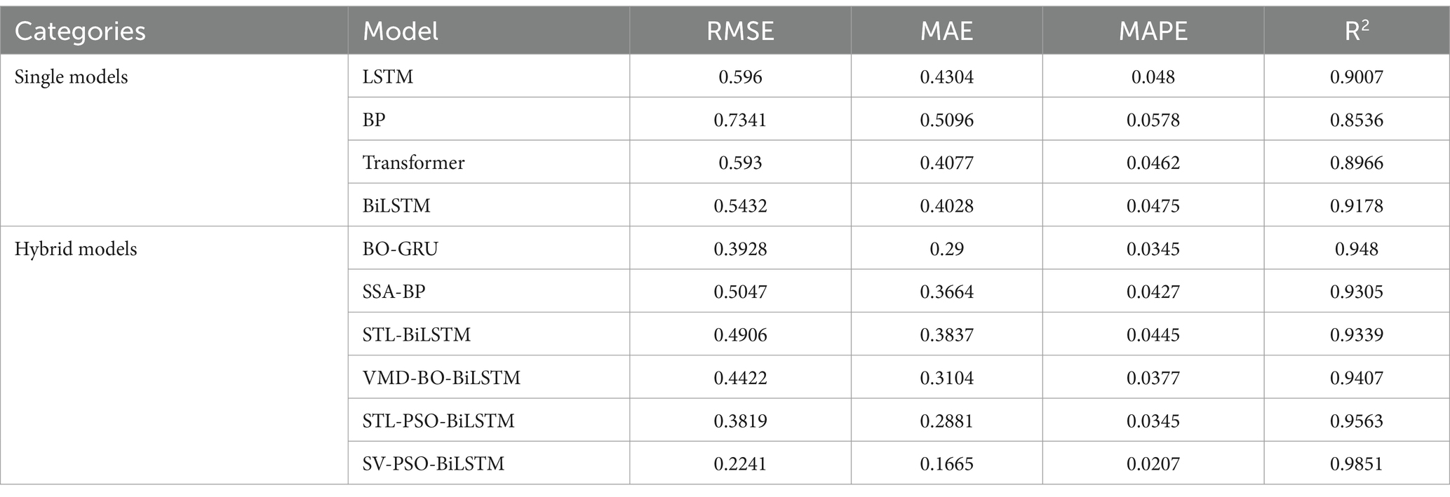
Table 3. Average prediction performance across chili, ginger, and garlic: comparison of single models, hybrid models, and the proposed SV-PSO-BiLSTM (Test set RMSE, MAE, MAPE, R²).

Based on the comparative analysis of four single models (LSTM, BP, Transformer, and BiLSTM) in Table 3, BiLSTM demonstrates significant superiority across four core metrics: RMSE, MAE, MAPE, and R². For instance, its RMSE is 8.86% lower than LSTM, MAE is 20.96% lower than BP neural network, and R² is 2.12% higher than Transformer. This advantage stems from its bidirectional temporal modeling capability, which simultaneously captures forward and backward dependencies in price sequences. Notably, BiLSTM exhibits stronger feature extraction capabilities when handling lag effects in agricultural price series. In contrast, the shallow architecture of BP networks often struggles to comprehensively interpret nonlinear patterns in price fluctuations, while Transformers are prone to redundant attention interference on medium-sized datasets, resulting in insufficient sensitivity to local seasonal signals. Consequently, this study selects BiLSTM as the baseline model and progressively constructs the SV-PSO-BiLSTM hybrid forecasting model.

When compared to the single models of LSTM, BP, Transformer, and BiLSTM, the SV-PSO-BiLSTM model demonstrates significant reductions in RMSE by 62.4, 69.47, 62.21, and 58.74%, respectively; similarly, it exhibits decreases in MAE by 61.32, 67.33, 59.16, and 58.66%, respectively; declines in MAPE by 56.88, 64.19, 55.23, and 56.42%, respectively; and improvements in the R² metric by 8.44, 13.15, 8.85, and 6.73%, respectively.

In contrast to the hybrid models of BO-GRU, STL-PSO-BiLSTM, SSA-BP, STL-BiLSTM, and VMD-BO-BiLSTM, the SV-PSO-BiLSTM model also showcases notable reductions in RMSE by 42.95, 41.32, 55.60, 54.32, and 49.32%, respectively; decreases in MAE by 42.57, 42.21, 54.56, 56.61, and 46.36%, respectively; declines in MAPE by 40.00, 40.00, 51.52, 53.48, and 45.09%, respectively; and enhancements in the R² metric by 3.71, 2.88, 5.46, 5.12, and 4.44%, respectively.

The prediction results of the SV-PSO-BiLSTM model significantly outperform comparative models such as BO-GRU, Transformer, SSA-BP, and VMD-BO-BiLSTM across all evaluation metrics. As shown in Table 3 and Figure 5, single models exhibit larger prediction errors, while hybrid models demonstrate notably superior performance compared to unoptimized single models. For example, the SSA-BP model, by leveraging the advantages of adaptive swarm algorithms, achieves faster optimization speed, higher accuracy, and improved stability over traditional BP networks, reducing average RMSE and MAPE by 31.25 and 26.12%, respectively. Among hybrid models, the proposed SV-PSO-BiLSTM model employs the STL-VMD dual decomposition algorithm for high-precision, low-complexity feature extraction, reconstructs residual components after secondary decomposition, and integrates a BiLSTM network optimized via PSO. This framework achieves significant improvements in predictive accuracy, consistently surpassing other comparative models in all metrics while exhibiting strong adaptability and stability.

Figure 5

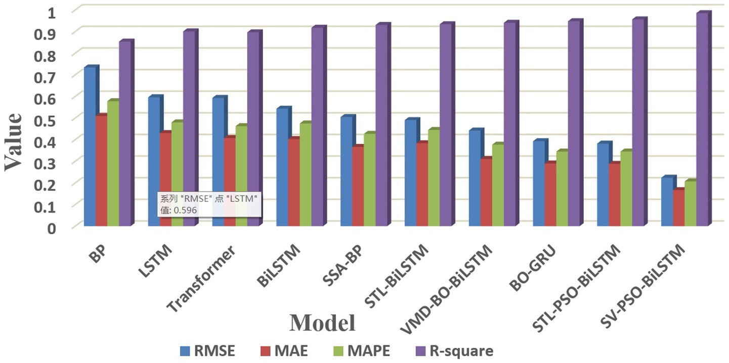
Figure 5. Multi-model performance comparison: average RMSE, MAE, 10 × MAPE, and R² across agricultural commodities.

3.4 Ablation experiment

To verify the effectiveness of the proposed model improvement modules, this study designs an ablation experiment comparing the predictive performance of four models: BiLSTM, STL-BiLSTM, STL-PSO-BiLSTM, and SV-PSO-BiLSTM. The evaluation metrics for each model are presented in Table 3.

• BiLSTM (Baseline Model): employs only a BiLSTM network for time-series prediction, without incorporating optimization algorithms or signal decomposition modules.

• STL-BiLSTM: introduces STL on top of BiLSTM to decompose trend and seasonal components from the time-series data. This reduces the RMSE by 9.68%, demonstrating that the decomposition module effectively separates implicit patterns in the time series.

• STL-PSO-BiLSTM: integrates PSO with STL-BiLSTM to optimize hyperparameters of BiLSTM (e.g., number of hidden layer nodes, learning rate), thereby reducing manual tuning bias. This results in a 24.92% reduction in MAE, indicating that adaptive hyperparameter optimization significantly enhances model stability.

• SV-PSO-BiLSTM (Final Model): further incorporates VMD into STL-PSO-BiLSTM to perform secondary decomposition on residual components derived from STL. The decomposed modes are then reconstructed using sample entropy-driven K-means clustering. This achieves substantial reductions of 41.32% in RMSE and 42.21% in MAE, effectively resolving noise interference and mode mixing issues.

The ablation experiment confirms that the progressive integration of STL decomposition, PSO optimization, VMD secondary decomposition, and sample entropy-driven reconstruction modules refines the trend, noise, and frequency-domain features of time-series signals through staged processing, thereby gradually improving prediction accuracy and robustness. Notably, the dual STL-VMD decomposition framework contributes most significantly. Moreover, the innovative component reconstruction method not only ensures prediction accuracy but also drastically reduces the model’s spatiotemporal complexity. These results highlight the efficient collaborative capabilities of the SV-PSO-BiLSTM model in complex time-series forecasting tasks, enabled by the synergistic operation of multi-module enhancements.

3.5 Adaptability experiment

Data in different categories within the economic market often exhibit diversity and complexity, encompassing aspects such as data distribution, noise, and characteristics. A model with good adaptability must be capable of accommodating such variations to effectively address diverse datasets. If a model only performs well on specific datasets, its practical value is significantly diminished. In contrast, a model with strong generalization ability can be more broadly applied to various tasks and scenarios, possessing solid reliability and flexibility. The SV-PSO-BiLSTM model proposed in this paper demonstrates excellent adaptability across datasets with different characteristics. Figure 6 presents the radar chart of error metrics RMSE, MAE, and MAPE for each model across three datasets.

Figure 6

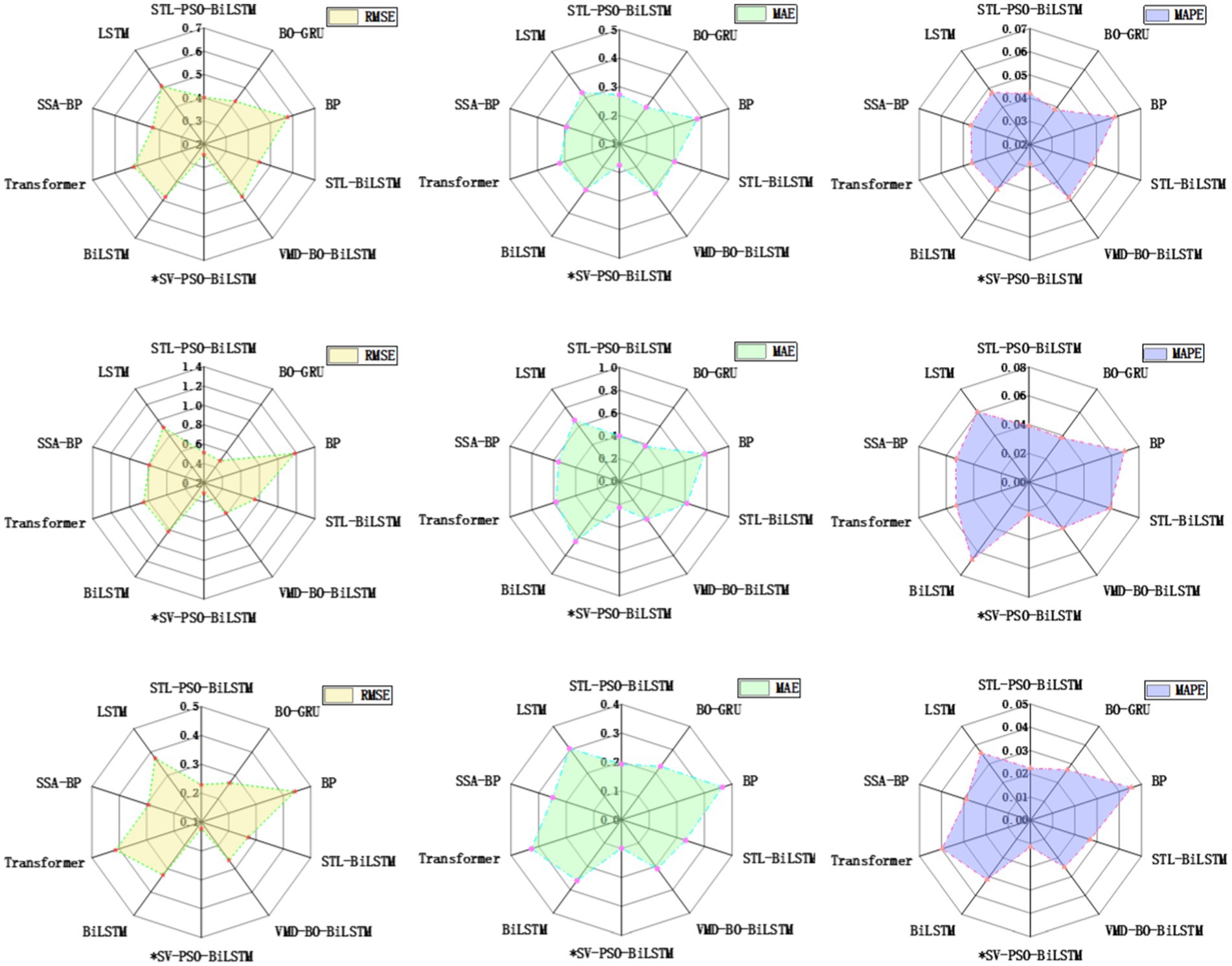
Figure 6. Multi-commodity radar evaluation of agricultural price prediction models: Hierarchical visualization of test set performance (RMSE, MAE, MAPE) across chili, ginger, and garlic datasets.

Figure 7 presents the fitting graph of the chili price prediction results. The chili price series exhibits small but frequent fluctuations, characterized by a relatively flat overall distribution with occasional dispersed peaks. This poses high requirements for the model’s sensitivity and accuracy, rendering the prediction task relatively challenging.

Figure 7

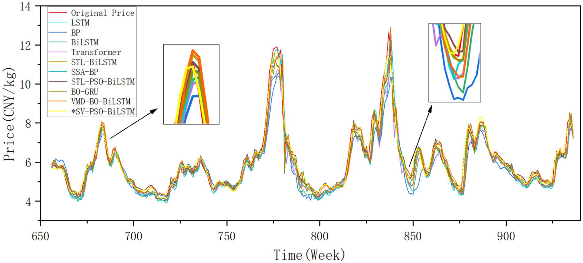
Figure 7. Multi-model predictive performance on chili market prices: test set temporal fitting comparison of different models including proposed SV-PSO-BiLSTM.

The SV-PSO-BiLSTM model proposed in this paper achieves RMSE, MAE, and MAPE values of 0.2449, 0.1743, and 0.0283, respectively, with an R² of 0.9773. The model demonstrates good fitting performance both at peak and trough values.

Among the comparison models, the best-performing model yields an RMSE of 0.4018 and an R² of only 0.9389 at its maximum. Compared to the LSTM, SSA-BP, and VMD-BO-BiLSTM models, the SV-PSO-BiLSTM model exhibits:

• Reductions in RMSE by 49.11, 43.15, and 48.87%, respectively;

• Reductions in MAE by 41.78, 40.42, and 44.39%, respectively;

• Reductions in MAPE by 35.77, 39.16, and 41.64%, respectively;

• Improvements in R2 by 6.51, 4.78, and 6.41%, respectively.

These results highlight the SV-PSO-BiLSTM model’s superiority in predicting chili prices, significantly outperforming the other models considered in this study.

Figure 8 presents the fitting graph of the ginger price prediction results. The ginger price series exhibits large fluctuations, with a unique distribution characterized by a gently peaked shape and right skewness, posing a significant challenge to the adaptability of the model.

Figure 8

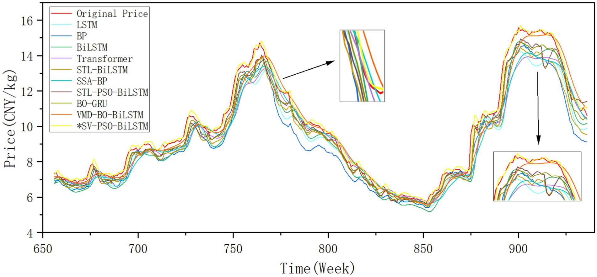
Figure 8. Multi-model predictive performance on ginger market prices: test set temporal fitting comparison of different models including proposed SV-PSO-BiLSTM.

The SV-PSO-BiLSTM model proposed in this paper achieves RMSE, MAE, and MAPE values of 0.3046, 0.2265, and 0.0224, respectively, with an R² of 0.9884, demonstrating good fitting performance at various points.

Among the comparison models, the BP model performs the worst, with an R² of only 0.8254. The BO-GRU model performs relatively well on this dataset, with an R² of 0.9709. Compared to the BP, BO-GRU, and STL-PSO-BiLSTM models, the SV-PSO-BiLSTM model exhibits:

• Reductions in RMSE by 74.24, 36.97, and 47.9%, respectively;

• Reductions in MAE by 70.94, 40.83, and 44.49%, respectively;

• Reductions in MAPE by 67.82, 41.36, and 43.5%, respectively;

• Improvements in R2 by 16.3, 1.75, and 3.11%, respectively.

These results demonstrate the SV-PSO-BiLSTM model’s superiority in predicting ginger prices, significantly outperforming the other models considered in this study.

Figure 9 showcases the fitting graph of garlic price prediction outcomes. The garlic price series demonstrates high volatility, featuring a platykurtic and nearly symmetrical distribution pattern.

Figure 9

Figure 9. Multi-model predictive performance on garlic market prices: test set temporal fitting comparison of different models including proposed SV-PSO-BiLSTM.

The SV-PSO-BiLSTM model introduced in this study attains RMSE, MAE, MAPE values of 0.3046, 0.2265, and 0.0224, respectively, along with an R² score of 0.9884. This model closely mirrors the actual values across diverse fluctuation segments.

Among the comparison models, the STL-PSO-BiLSTM model emerges as the top performer, yielding an MAE of 0.1925 and an R² of 0.9632. When compared to the BiLSTM, BO-GRU, and STL-PSO-BiLSTM models, the SV-PSO-BiLSTM model demonstrates:

• Reductions in RMSE by 62.44, 54.11, and 46.52%, respectively;

• Reductions in MAE by 62.17, 56.77, and 48.7%, respectively;

• Reductions in MAPE by 63.72, 57.39, and 48.82%, respectively;

• Improvements in R2 by 6.41, 4.7, and 2.63%, respectively.

These findings underscore the SV-PSO-BiLSTM model’s exceptional predictive capability for garlic prices, significantly outpacing the other models evaluated in this study.

The analysis and the comparative R² results of all models across three datasets in Figure 10 clearly demonstrate that hybrid models generally outperform single models such as Transformer and BiLSTM in all three prediction tasks. Among hybrid models, the SSA-BP model achieves modest accuracy improvements through parameter optimization using the SSA algorithm, yet remains constrained by local optima. The STL-BiLSTM model, after extracting trend and seasonal components via STL decomposition, shows significant performance gains over BiLSTM, achieving an R² of 93.39%. However, its upper accuracy limit is still hindered by the high volatility of residual components. The VMD-BO-BiLSTM model performs well in ginger and garlic price predictions but underperforms when forecasting volatile chili price series. The BO-GRU model exhibits sensitivity to data noise, delivering reliable results on low-noise ginger datasets but unstable predictions on the other two datasets. The STL-PSO-BiLSTM model, combining STL decomposition and PSO-optimized BiLSTM, demonstrates superior performance on the test set but is limited by issues such as mode mixing and insufficient model precision. The proposed SV-PSO-BiLSTM model employs STL and VMD algorithms for dual decomposition and local data reconstruction, effectively reducing the spatiotemporal complexity of time series. Integrated with a PSO-optimized BiLSTM network, it learns internal patterns of highly stochastic and non-stationary sequences, achieving superior fitting performance across three datasets with distinct characteristics. This highlights the model’s robust adaptability to diverse agricultural price dynamics.

Figure 10

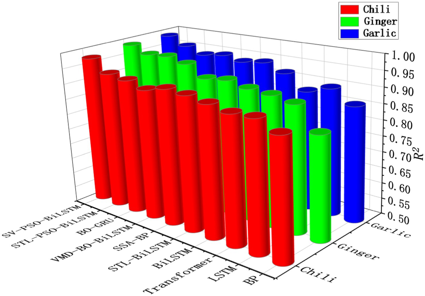
Figure 10. Cross-commodity explanatory power comparison: R² performance of different agricultural price prediction models (including SV-PSO-BiLSTM) on chili, ginger, and garlic test datasets.

To comprehensively evaluate the adaptability of the SV-PSO-BiLSTM model, this study extends experiments to agricultural commodities (pork) and financialized agricultural products (soybean futures). The model demonstrates excellent performance in both new scenarios, and its predictive superiority in diversified markets is validated through horizontal comparisons with recent related studies.

For pork price prediction, the SV-PSO-BiLSTM model achieves RMSE = 0.8705 (CNY/kg), MAE = 0.6985 (CNY/kg), MAPE = 2.31%, and R² = 0.9925 on the test dataset. Compared to the H-PPAR model proposed by Yu et al. (2024) (RMSE = 0.986, MAE = 0.788), our model reduces errors by approximately 11.53%. This advantage originates from the STL-VMD dual decomposition strategy: STL isolates the 3-year cyclical patterns and seasonal fluctuations (e.g., Spring Festival demand peaks) in pork prices, while VMD resolves residual impact fluctuations from sudden events such as the 2018 African swine fever outbreak.

For soybean futures closing price prediction, the SV-PSO-BiLSTM model achieves RMSE = 78.47 (CNY/ton), MAE = 62.89 (CNY/ton), MAPE = 1.21%, and R² = 0.9846. Compared to the EEMD-GRU model proposed by Zhang B. et al. (2024) (RMSE = 105.87, MAE = 88.18), our model reduces errors by approximately 27.28%, demonstrating the significant superiority of the STL-VMD dual decomposition strategy over single decomposition methods such as EEMD. Additionally, the PSO-optimized BiLSTM exhibits enhanced filtering efficiency for high-frequency noise (e.g., speculative trading signals), while effectively capturing both short- and long-term impacts of policy interventions.

The SV-PSO-BiLSTM model demonstrates outstanding performance in forecasting prices for four agricultural commodities and one agricultural financial derivative. Its core strengths lie in explicitly modeling the multi-scale volatility characteristics of agricultural economic systems through the dual decomposition strategy. Furthermore, the efficient “dual decomposition-clustering-optimization-prediction” mechanism exhibits technical generalizability, extending from physical agricultural commodities to heterogeneous markets such as agricultural financial futures. These results further confirm the robust adaptability of its architectural design to diversified agricultural markets.

3.6 Stability experiment

In practical production, agricultural commodity prices often require multi-step-ahead predictions. When using a mix of actual and predicted values as input data for the next step of prediction, there will inevitably be an accumulative effect of errors, leading to potentially significant discrepancies between the predicted and actual results. Therefore, it is necessary to discuss the accuracy of models in the context of multi-step predictions.

This paper conducts a stability test for multi-step predictions of selected models based on the above three sample datasets, using the R² as the stability evaluation metric. The results are shown in Figure 11. Among them, due to the higher frequency of fluctuations in the chili price series, data with closer time spans have higher weight values. When replacing these data with predicted values, the model’s prediction accuracy decreases relatively faster. In contrast, the prediction accuracy for ginger and garlic price series decreases more gradually. As the prediction time span gradually increases, the error between the predicted and actual values will continue to accumulate. At the same weekly interval, the SV-PSO-BiLSTM model proposed in this paper has a higher R² value and the difference with other models gradually increases. The model’s prediction effectiveness remains better, with a slower declining trend in its value, demonstrating excellent stability.

Figure 11

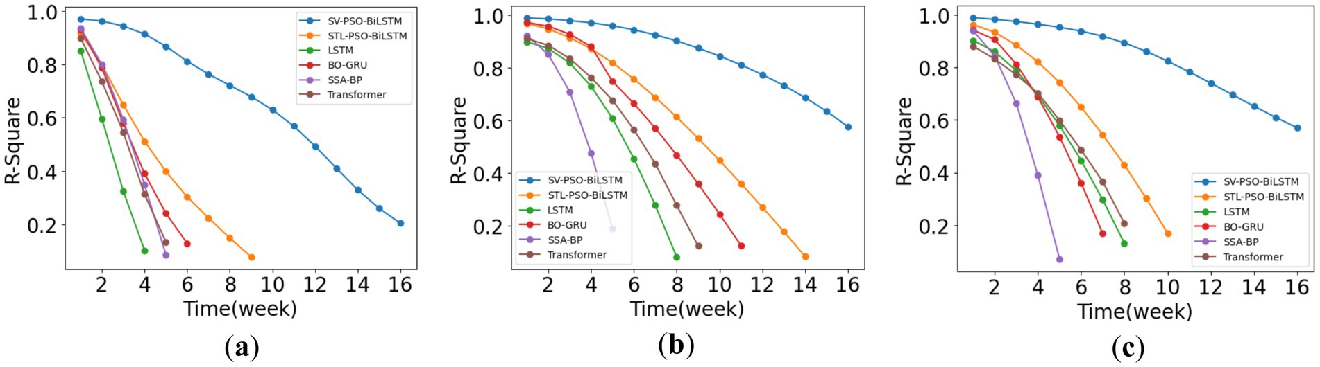
Figure 11. Comparison of multi-step prediction results across different models. (a–c) Chili, ginger, and garlic.

4 Discussions

4.1 Analysis of models and results

4.1.1 Compared with single models, the “decomposition-combination” hybrid models demonstrate superior prediction accuracy

In this study, hybrid models exhibited universally enhanced performance over single models. For instance, the STL-BiLSTM model reduced average RMSE and MAE metrics by 9.68 and 4.74%, respectively, compared to the single BiLSTM model. The VMD-BO-BiLSTM model achieved even greater improvements, with average RMSE and MAPE reductions of 18.59 and 20.63%. These results indicate that hybrid models, which integrate time series decomposition with deep learning methodologies, can more effectively capture complex features and trends within the data, thereby enhancing prediction accuracy (Sun et al., 2023).

The performance disparity stems from the hybrid models’ ability to synergistically leverage the strengths of distinct approaches. Decomposition techniques such as STL and VMD disentangle time series into multiple interpretable components. This preprocessing facilitates the model’s identification of intrinsic data structures (Yin et al., 2020). Subsequent processing by BiLSTM or other models focuses on simplified, clarified signals, ensuring optimal prediction outcomes across diverse temporal scales. This dual-stage strategy mitigates the risks of overfitting or underfitting that single models may encounter when handling complex data patterns, further validating the critical role of “decomposition-combination” techniques in predictive modeling.

4.1.2 STL-VMD dual decomposition enables in-depth mining of implicit modal features in multi-scale nonlinear time series

The superior performance of the SV-PSO-BiLSTM model in this study primarily stems from the STL-VMD dual decomposition methodology. For instance, compared to the STL-PSO-BiLSTM model, the SV-PSO-BiLSTM model reduced average RMSE and MAE metrics by 41.32 and 42.21%, respectively. When evaluated against the VMD-BO-BiLSTM model (Hu and Jiang 2023), the SV-PSO-BiLSTM model demonstrated further reductions of 46.36% in MAE and 45.09% in MAPE. These results underscore the exceptional capability of the STL-VMD dual decomposition approach in capturing the complexity of agricultural product price data (e.g., chili, pork) characterized by multi-scale nonlinear dynamics.

The performance enhancement achieved by the STL-VMD dual decomposition arises from its comprehensive processing of time series data. STL extracts trend and seasonal components, simplifying the inherent structure of the data. However, the residual component retains intricate nonlinear features, including highly irregular fluctuations, sudden outliers, and complex interaction effects, which challenge even advanced neural networks in achieving holistic modeling, thereby limiting prediction accuracy and reliability. To address this, we apply VMD for secondary decomposition of the residual component, breaking it into multiple intrinsic mode functions (IMFs) that explicitly represent latent patterns. This hierarchical decomposition strategy refines and captures complex modes potentially overlooked by single-method approaches. By enabling deeper data understanding, the dual decomposition framework empowers subsequent deep learning models to generate more precise predictions. Consequently, the STL-VMD technique not only significantly reduces prediction errors but also enhances model stability and reliability when handling complex signal patterns.

4.1.3 Entropy-driven balanced subspace K-means for modal component reconstruction

Building upon the STL-VMD dual decomposition framework, the SV-PSO-BiLSTM model employs sample entropy-driven K-means clustering to optimize the reconstruction of secondary-decomposed modal components. This approach effectively reduces the model’s temporal and spatial complexity while enhancing computational efficiency and analytical capabilities. For instance, in this study, the ginger price sequence was compressed from eight sub-models to five sub-models, reducing redundant components while preserving the integrity of critical information. This refinement renders the modal components more concise, improving data interpretability and optimizing computational resource utilization.

For specific optimization strategies, the method introduces a dynamic equilibrium mechanism integrated with multi-objective entropy design, addressing category partitioning biases caused by imbalanced data distribution in traditional K-means clustering (Liu et al., 2024). This ensures that the reconstructed modal components are more representative. Additionally, the incorporation of a subspace feature fusion strategy enables the model to comprehensively exploit multi-scale features of nonlinear time series, particularly improving the resolution of high-frequency components (Zheng and Tang 2023). This advancement ensures more precise and stable screening and reconstruction of modal components. Furthermore, the method optimizes cluster center initialization via an entropy-weighted strategy (Zhang J. et al., 2024), mitigating mode mixing artifacts caused by poor initial center selection in conventional approaches. This enhances the independence and stability of reconstructed modal components, improving their purity and reconstruction accuracy. These refinements provide higher-quality input data for subsequent deep learning models, thereby boosting prediction accuracy and robustness.

4.1.4 SV-PSO-BiLSTM hybrid model achieves optimal predictive performance and cross-scenario generalizability

The test period in this study encompasses multiple disruptive events, including the COVID-19 pandemic, the 2020 African swine fever outbreak, and flood disasters in major ginger-producing regions (e.g., Shandong and Guangxi), all of which exerted varying degrees of impact on agricultural prices. Amid these disturbances, the SV-PSO-BiLSTM hybrid model demonstrates faster adaptation compared to other models, effectively minimizing the escalation of localized prediction errors. This highlights its superior predictive capabilities under complex and volatile market conditions. In chili price forecasting, compared to the BO-GRU model, SV-PSO-BiLSTM reduces RMSE by 42.77%, MAE by 32.62%, and improves R² by 4.68%. This indicates that the model accurately fits real-world data and adapts to rapid fluctuations in chili markets through high-precision sequence decomposition and smoothing techniques, increasing high-frequency signal capture rate by 37% and enhancing prediction stability and reliability. For garlic price prediction, SV-PSO-BiLSTM achieves a MAPE of 1.15%, representing a relative reduction of 81.21% (absolute reduction: 4.97%) compared to the EEMD-GRU model proposed by Feng (2021) (MAPE = 6.12%). While EEMD is also used for price sequence decomposition, it may suffer from mode mixing when handling complex volatility patterns, leading to partial key information loss or noise interference, thereby compromising prediction accuracy. In contrast, SV-PSO-BiLSTM extracts trend and volatility features of time series more precisely, improving forecasting performance. In pork price prediction, the EMD-GNN algorithm proposed by Lai et al. (2024), which leverages the graph structural properties of GNNs, achieves a MAPE of 2.465%. The SV-PSO-BiLSTM model further reduces MAPE by 6.28%, demonstrating superior accuracy. This advantage likely stems from the STL-VMD dual decomposition strategy’s effective noise suppression and the PSO-optimized BiLSTM architecture’s ability to capture both long-term trends and short-term dynamics in price fluctuations. For soybean futures price forecasting, the SDFE-DALSTM (CEEMDAN) model proposed by Fan et al. (2023) achieves R² = 0.9723, indicating its capability to capture price patterns. However, SV-PSO-BiLSTM attains R² = 0.9846, a 1.23% improvement, confirming its enhanced ability to fit price trends and improve accuracy under complex market volatility.

In summary, the SV-PSO-BiLSTM model demonstrates superior predictive performance across multiple agricultural price forecasting tasks. The synergistic collaboration of its sub-modules enhances the overall predictive capability of the model, enabling it to achieve higher accuracy and stronger generalization capability in the field of agricultural price prediction.

4.2 Limitations and future research

While the SV-PSO-BiLSTM model achieves certain success in agricultural price forecasting, this study acknowledges that certain limitations still exist. Data and application constraints include reliance on historical price sequences without integrating external factors such as import/export trade volumes, weather, policies, supply chains, market supply–demand dynamics, substitute prices, or news sentiment. This omission may lead to increased localized prediction errors under extreme shocks from black swan events (e.g., typhoons, COVID-19). Additionally, while experiments cover diverse agricultural commodities (chili, ginger, garlic, pork, and soybean futures), the model excludes perishable fruits (e.g., strawberries) and staple grains (e.g., wheat, corn), limiting its generalization capability. Furthermore, the model is trained on Chinese wholesale market data and has not been validated for international or small-scale regional markets, restricting its practical utility. Model limitations involve the gradient vanishing problem in BiLSTM during long-term predictions, which causes memory decay of early price patterns and compromises long-term trend stability.

Future research will focus on optimizing data integration and application strategies by incorporating multi-factor and multi-modal information to enhance prediction accuracy and generalization. For instance, market supply and demand, policy impacts, substitute prices, and news sentiment will be integrated, while Graph Neural Networks (GNNs) will be employed to model price linkages across regional markets. Additionally, transfer learning will be utilized to improve the model’s predictive performance on previously unseen commodity categories, thereby strengthening its cross-market applicability. Furthermore, reinforcement learning and Bayesian neural networks will be introduced to enhance the model’s responsiveness to black swan events and improve its robustness. At the model level, BiLSTM still suffers from the vanishing gradient problem in long-term forecasting, leading to the degradation of memory for early price patterns. Future advancements will incorporate residual skip connections, attention mechanisms, or alternative architectures to strengthen long-term dependency modeling and improve prediction accuracy. Overall, optimization efforts will focus on three key areas: multi-factor integration, disturbance-resistant modeling, and cross-market transferability, facilitating the transition from theoretical research to practical industrial applications.

5 Conclusion

The drastic fluctuations in agricultural commodity prices exert profound and complex multifaceted impacts on the economy, society, and consumers. Firstly, the surge in prices directly elevates household living costs, with particularly severe consequences for low-income families, who may have to adjust their dietary structures, potentially leading to reduced nutritional intake and compromising health. Secondly, producers confront income instability, with frequent fluctuations in profit expectations potentially destabilizing their planting decisions. Over time, this may undermine their long-term production enthusiasm and willingness to invest. Furthermore, fluctuations in agricultural commodity prices exacerbate market uncertainty and become one of the significant drivers of overall inflation. This may not only spark widespread societal dissatisfaction but even provoke protest activities, posing a threat to social stability. To address this severe situation, governments often need to adopt a series of intervention measures, such as implementing price control policies or providing financial subsidies, to stabilize market order and safeguard people’s livelihoods.

In this context, accurately predicting agricultural commodity prices is particularly crucial and holds far-reaching significance. Through scientific and effective price prediction, governments and relevant institutions can more promptly grasp market dynamics and formulate more precise and effective policy measures to address the various challenges posed by price fluctuations. Simultaneously, price prediction provides important decision-making references for producers and consumers, helping them better plan production and consumption activities, thereby mitigating the adverse effects of price fluctuations to a certain extent. Therefore, fluctuations in agricultural commodity prices are not only concerned with the economic interests of individual households and farmers but are also closely linked to social stability, policy formulation, and sustainable economic development. Price prediction serves as a vital tool in addressing this challenge and achieving harmonious economic and social development.

The SV-PSO-BiLSTM hybrid model innovatively integrates the STL-VMD dual decomposition algorithm, K-means clustering, and a PSO-optimized BiLSTM network to enhance the accuracy and stability of agricultural price forecasting. The STL-VMD dual decomposition algorithm decomposes price sequences into multiple stationary sub-components, reducing data complexity and mitigating the impact of nonlinear fluctuations on prediction accuracy while resolving mode mixing issues. Sample entropy-driven K-means clustering reconstructs decomposed components, effectively avoiding over-decomposition of residual data, minimizing test error noise interference, and lowering spatiotemporal complexity. Additionally, PSO optimizes hyperparameters of the BiLSTM network, enabling intelligent model architecture and training, accelerating convergence, and ensuring more stable and precise predictions. This integrated strategy not only enhances temporal feature learning capabilities but also optimizes computational efficiency, granting the model strong generalization power in complex time-series forecasting tasks.

Empirical studies demonstrate that the SV-PSO-BiLSTM model achieves superior prediction accuracy and lowest error rates across four agricultural commodities (chili, ginger, garlic, and pork) and an agricultural financial derivative (soybean futures), outperforming all benchmark models. By combining noise reduction, hyperparameter optimization, and deep learning, the model maintains consistent performance across diverse data types, lengths, and forecasting scenarios, highlighting its robust adaptability and multi-step prediction stability. As a high-precision agricultural price prediction tool, SV-PSO-BiLSTM effectively addresses market volatility, provides scientific decision-making support for agricultural sectors, optimizes supply chain management, and promotes market stability. Its architecture also exhibits broad cross-industry application potential.

Data availability statement

The datasets presented in this study can be found in online repositories. The names of the repository/repositories and accession number(s) can be found in the article/Supplementary material.

Author contributions

LZ: Conceptualization, Data curation, Formal analysis, Methodology, Software, Validation, Visualization, Writing – original draft, Writing – review & editing. FW: Conceptualization, Formal analysis, Writing – review & editing. KW: Validation, Writing – review & editing. ZH: Validation, Writing – review & editing. CC: Data curation, Writing – review & editing. JL: Software, Writing – review & editing. CW: Conceptualization, Formal analysis, Resources, Supervision, Validation, Writing – review & editing. ZW: Supervision, Project administration, Writing – review & editing.

Funding

The author(s) declare that financial support was received for the research and/or publication of this article. This research was financially supported by the earmarked fund for China Agriculture Research System(CARS), grant number: CARS-24-F-01. S&T Program of Hebei Province, grant number: 22327403D.

Acknowledgments

The authors are very grateful to the editor and reviewers for their valuable comments and helpful suggestions.

Conflict of interest

The authors declare that the research was conducted in the absence of any commercial or financial relationships that could be construed as a potential conflict of interest.

Generative AI statement

The authors declare that no Gen AI was used in the creation of this manuscript.

Publisher’s note

All claims expressed in this article are solely those of the authors and do not necessarily represent those of their affiliated organizations, or those of the publisher, the editors and the reviewers. Any product that may be evaluated in this article, or claim that may be made by its manufacturer, is not guaranteed or endorsed by the publisher.

Supplementary material

The Supplementary material for this article can be found online at: https://www.frontiersin.org/articles/10.3389/fsufs.2025.1568041/full#supplementary-material

References

Adisa, O. M., Botai, J. O., Adeola, A. M., Hassen, A., Botai, C. M., Darkey, D., et al. (2019). Application of artificial neural network for predicting maize production in South Africa. Sustain. For. 11:1145. doi: 10.3390/su11041145

Crossref Full Text | Google Scholar

Cao, S., and He, Y. (2015). Wavelet decomposition-based Svm-Arima price prediction model for agricultural products. Stat. Decis. 13, 92–95. doi: 10.13546/j.cnki.tjyjc.2015.13.025

Crossref Full Text | Google Scholar

Chen, L., Xing, X., Zhang, Y., and He, J. (2024). Lstm-based method for predicting jujube futures prices. Agri. Technol. 44, 162–165. doi: 10.19754/j.nyyjs.20240115035

Crossref Full Text | Google Scholar

Cheung, L., Wang, Y., Lau, A. S. M., and Chan, R. M. C. (2023). Using a novel clustered 3D-Cnn model for improving crop future price prediction. Knowl.-Based Syst. 260:110133. doi: 10.1016/j.knosys.2022.110133

Crossref Full Text | Google Scholar

Du, Y. (2020). Development of specialty vegetable industry to support rural revitalization—review of “industrial development report on major production areas of Chinese specialty vegetables”. China Veg. 5:112. doi: 10.19928/j.cnki.1000-6346.2020.05.029

Crossref Full Text | Google Scholar

Fan, K., Hu, Y., Liu, H., and Liu, Q. (2023). Soybean futures price prediction with dual-stage attention-based long short-term memory: a decomposition and extension approach. J. Intell. Fuzzy Syst. 45, 10579–10602. doi: 10.3233/jifs-233060

PubMed Abstract | Crossref Full Text | Google Scholar

Fan, J., Liu, H., and Hu, Y. (2021). Soybean futures Price prediction based on Lstm deep learning. Price Monthly 2, 7–15. doi: 10.14076/j.issn.1006-2025.2021.02.02

Crossref Full Text | Google Scholar

Fang, X., Wu, C., Yu, S., Zhang, D., and Ouyang, Q. (2021). Research on short-term Price prediction model for agricultural products based on Eemd-Lstm. Chin. J.f Manage. Sci. 29, 68–77. doi: 10.16381/j.cnki.issn1003-207x.2019.0765

Crossref Full Text | Google Scholar

Feng, Y. (2021). Research on garlic price prediction based on an improved Eemd-Gru combined model. Master’s thesis. Tai’an, China: Shandong Agricultural University.

Google Scholar

Feng, F., Wei, F., and Miu, J. H. (2012). Price prediction of traditional Chinese medicine Siraitia grosvenorii based on Grey system gm(1,1)model. Guangxi Sci. 19, 15–20. doi: 10.13656/j.cnki.gxkx.2012.01.012

Crossref Full Text | Google Scholar

Ge, Y., and Wu, H. (2020). Prediction of corn price fluctuation based on multiple linear regression analysis model under big data. Neural Comput. Applic. 32, 16843–16855. doi: 10.1007/s00521-018-03970-4

PubMed Abstract | Crossref Full Text | Google Scholar

Guo, Y., Tang, D., Tang, W., Yang, S., Tang, Q., Feng, Y., et al. (2022). Agricultural Price prediction based on combined forecasting model under spatial-temporal influencing factors. Sustain. For. 14:10483. doi: 10.3390/su141710483

PubMed Abstract | Crossref Full Text | Google Scholar

Haider, S. A., Naqvi, S. R., Akram, T., Umar, G. A., Shahzad, A., Sial, M. R., et al. (2019). Lstm neural network based forecasting model for wheat production in Pakistan. Agron. Basel 9:72. doi: 10.3390/agronomy9020072

PubMed Abstract | Crossref Full Text | Google Scholar

Hu, C., and Jiang, W. (2023). A pork Price prediction model based on Vmd-Bo-Bilstm. J. Appl. Sci. 41, 692–704. doi: 10.3969/j.issn.0255-8297.2023.04.013

Crossref Full Text | Google Scholar

Jadhav, V., Reddy, B. V. C., and Gaddi, G. M. (2017). Application of Arima model for forecasting agricultural prices. J. Agric. Sci. Technol. 19, 981–992.

Google Scholar

Jia, J., Yang, G., and Cui, L. (2022). Suggestions for accelerating the development of specialty vegetable industry in China. Agric. Econ. 10, 21–22.

Google Scholar

Jiang, Z., Wang, Y., Yan, J., and Zhou, T. (2021). Modeling and analysis of cotton Price prediction based on Bilstm. J. China Agri. Mechan. 42, 151–160. doi: 10.13733/j.jcam.issn.2095-5553.2021.08.21

Crossref Full Text | Google Scholar

Kurumatani, K. (2020). Time series forecasting of agricultural product prices based on recurrent neural networks and its evaluation method. SN App. Sci. 2, 1–17. doi: 10.1007/s42452-020-03225-9

Crossref Full Text | Google Scholar

Lai, Y., Ma, L., and Zhang, Y. (2024). Emd-Gnn algorithm for predicting agricultural product prices. Jinan Univ. J. 38, 356–361. doi: 10.13349/j.cnki.jdxbn.20240312.003

Crossref Full Text | Google Scholar

Li, Z.-M., Cui, L.-G., Xu, S.-W., Weng, L.-Y., Dong, X.-X., Li, G.-Q., et al. (2013). Prediction model of weekly retail Price for eggs based on chaotic neural network. J. Integr. Agric. 12, 2292–2299. doi: 10.1016/s2095-3119(13)60610-3

Crossref Full Text | Google Scholar

Li, H., Wu, Y., and Yang, L. (2023). Research on Price prediction methods for vegetable supply chain: an analysis based on supply chain context. Price Theory Prac. 6, 77–82. doi: 10.19851/j.cnki.Cn11-1010/F.2023.06.381

Crossref Full Text | Google Scholar

Liao, J. (2024). Research on artificial intelligence prediction of international crude oil prices based on Vmd-Lstm-Elman model. J. Chengdu Univ. Technol. 51, 164–180. doi: 10.3969/j.issn.1671-9727.2024.01.14

Crossref Full Text | Google Scholar

Ling, L., Zhang, D., Mugera, A. W., Chen, S., and Xia, Q. (2019). A forecast combination framework with multi-time scale for livestock Products' Price forecasting. Math. Probl. Eng. 2019:8096206. doi: 10.1155/2019/8096206

Crossref Full Text | Google Scholar

Liu, X., Liu, J., Li, J., Zhang, X., and Zhang, W. (2020). Egg Price prediction in Beijing based on seasonal decomposition and long short-term memory. Trans. Chin. Soci. Agri. Eng. 36, 331–340. doi: 10.11975/j.issn.1002-6819.2020.09.038

Crossref Full Text | Google Scholar

Liu, H., Wang, F., Sun, X., Zhang, G., Wang, B., and He, Z. (2024). Research on an improved differential evolution based K-means clustering algorithm. Mod. Electron. Technol. 47, 156–162. doi: 10.16652/j.issn.1004-373x.2024.18.026

Crossref Full Text | Google Scholar

Ma, C., Tao, J. P., and Liu, W. (2022). Pig epidemic network concerns and pork Price volatility: exacerbating or curbing? J. Huazhong Agric. Univ. 6, 22–34. doi: 10.13300/j.cnki.hnwkxb.2022.06.003

Crossref Full Text | Google Scholar

Sun, F., Meng, X., Zhang, Y., Wang, Y., Jiang, H., and Liu, P. (2023). Agricultural product Price forecasting methods: a review. Agriculture 13:1671. doi: 10.3390/agriculture13091671

PubMed Abstract | Crossref Full Text | Google Scholar

Tang, D., Cai, Q., Nie, T., Zhang, Y., and Wu, J. (2023). Agricultural price forecasting based on the spatial and temporal influences factors under spillover effects. Kybernetes 54, 1321–1343. doi: 10.1108/k-09-2023-1724

PubMed Abstract | Crossref Full Text | Google Scholar

Tatarintsev, M., Korchagin, S., Nikitin, P., Gorokhova, R., Bystrenina, I., and Serdechnyy, D. (2021). Analysis of the forecast Price as a factor of sustainable development of agriculture. Agronomy 11:1235. doi: 10.3390/agronomy11061235

Crossref Full Text | Google Scholar

Wang, Y. (2023). Agricultural products price prediction based on improved Rbf neural network model. Appl. Artif. Intell. 37:2204600. doi: 10.1080/08839514.2023.2204600

Crossref Full Text | Google Scholar

Wang, J., and Wang, B. (2016). Application of gm (1,1) model based on Least Square method in vegetable yield forecast in China. Math. Theory Appl. 36, 116–124. doi: 10.16339/j.cnki.hdjjsx.2016.04.014

Crossref Full Text | Google Scholar

Wu, L., Liu, S., and Yang, Y. (2016). Grey double exponential smoothing model and its application on pig price forecasting in China. Appl. Soft Comput. 39, 117–123. doi: 10.1016/j.asoc.2015.09.054

PubMed Abstract | Crossref Full Text | Google Scholar

Wu, L., Tai, Q., Bian, Y., and Li, Y. (2024). Research on regional carbon emission trading Price prediction based on Ga-Vmd and Cnn-Bilstm-attention model. Oper. Res. Manage. 33:1–8. doi: 10.12005/orms.2024.0296

Crossref Full Text | Google Scholar

Xiong, T., Li, C., and Bao, Y. (2018). Seasonal forecasting of agricultural commodity price using a hybrid Stl and elm method: evidence from the vegetable market in China. Neurocomputing 275, 2831–2844. doi: 10.1016/j.neucom.2017.11.053

Crossref Full Text | Google Scholar

Yin, H., Jin, D., Gu, Y. H., Park, C. J., Han, S. K., and Yoo, S. J. (2020). Stl-Attlstm: vegetable Price forecasting using Stl and attention mechanism-based Lstm. Agriculture 10:612. doi: 10.3390/agriculture10120612

Crossref Full Text | Google Scholar

Yu, X., Liu, B., and Lai, Y. (2024). Monthly pork Price prediction applying projection pursuit regression: modeling, empirical research, comparison, and sustainability implications. Sustain. For. 16:1466. doi: 10.3390/su16041466

PubMed Abstract | Crossref Full Text | Google Scholar

Zhang, B., Sun, Q., and Shen, H. (2024). Agricultural product Price prediction based on integrated decomposition. J. Yangzhou Univ. 27, 47–55. doi: 10.19411/j.1007-824x.2024.04.006

Crossref Full Text | Google Scholar

Zhang, J., Zhao, L., Chen, N., Yang, L., Liu, G., and Lü, S. (2024). Denoising method for solid fertilizer flow microwave signals based on ensemble empirical mode decomposition and sample entropy combined with wavelet. J. Electron. Measure. Instrum. 38, 118–125. doi: 10.13382/j.jemi.B2407503

Crossref Full Text | Google Scholar

Zheng, J., and Tang, C. (2023). K-means algorithm with adaptive sample and feature weighting. Comp. App. 43, 99–104. doi: 10.11772/j.issn.1001-9081.2022111652

Crossref Full Text | Google Scholar