 Darren Pouliot
 Niloofar Alavi
- Landscape Science and Technology Division, Environment and Climate Change Canada, National Wildlife Research Centre, Ottawa, ON, Canada
Effectively mapping and detecting changes in forests and linear woody features (LWFs) is crucial for assessing their impact on biodiversity and ecosystem services. This study investigated this capability using heterogeneous, high-resolution aerial imagery, in terms of spectral and spatial properties. Mitigating the influence of these factors, arising from differences in sensor specifications and acquisition conditions, is essential for robust detection and analysis of temporal change across historical image datasets. The deep learning model developed here successfully mapped forests and LWFs between 1954 and 2019 using just a single image band, enabling reliable change estimation. Assessment at the pixel scale showed forest mapping achieved an accuracy of 90%, while LWF accuracy was lower at 69%, primarily due to their narrow widths and boundary errors in both the reference and predicted results. For LWFs an object-based assessment was undertaken to reduce the effect of precise delineation achieving a higher accuracy of 77%. As a final assessment, comparison of area within 200 by 200 m extents showed good agreement, with a mean absolute error of 1.3% for LWFs. For forests this was 2.7%. In terms of change detection, the accuracy was greater than 81% for both forests and LWFs. Change analysis indicated an 8.5% net increase in forests since 1954, along with a small net loss of less than 1% in LWFs. LWF loss was mainly attributed to forest gains. In areas without significant forest gain, LWFs slightly increased. These changes are generally seen as beneficial for biodiversity and ecosystem services in the region. However, other factors such as urban development and larger agricultural field sizes need to be considered in future studies.
1 Introduction
Hedgerows or linear woody features (LWFs) are defined as linear strips of managed or unmanaged woody vegetation (shrubs and/or trees) on agricultural landscapes between and along cropped fields or roadways, rail corridors and watercourses (Pasher et al., 2016; Dover, 2019). According to the UK Countryside Survey a hedgerow should have a minimum length of 20 m and minimum width of 5 m, and if composed of trees, it should be one tree wide (Maskell et al., 2008). Statistics Canada (2021) considers shelterbelts, windbreaks, hedgerows, field margins, woodlots, riparian buffers and pivot corners with a width of less than 10 m as LWFs. The Small Woody Features product developed by the Copernicus Land Monitoring Service defines linear features as having a width less than 30 m and length greater than 30 m (EU, CLMS, EEA, 2021).
LWFs are considered a nature-based solution (Collier, 2021) and contribute various ecosystem services such as providing shelter from winds, reducing soil erosion, improving soil drainage (Benhamou et al., 2013); limiting evapotranspiration, preventing snowdrifts (Pasher et al., 2016; Collier, 2021); enhancing carbon storage (Axe et al., 2017; Biffi et al., 2022); increasing nitrogen retention (Benhamou et al., 2013); providing some pest control (Morandin et al., 2014; Long et al., 2017); and pollination services (Garratt et al., 2017; Long et al., 2017; Bishop et al., 2023; Boinot et al., 2023). In addition, they enhance biodiversity by providing food (Staley et al., 2012), shelter (Lecq et al., 2017), movement corridors (Fahrig et al., 2015; Dondina et al., 2016; Aviron et al., 2018; Clausen et al., 2022), and microclimates (Aviron et al., 2018; Lecq et al., 2018; Dover, 2019; Collier, 2021). They also provide human co-benefits such as foraging and hunting, and shading or sheltering buildings (Cole, 1955; Collier, 2021).
The diversity and abundance of species in agroecosystems is known to be influenced by LWFs including non-crop plants (McCann et al., 2017; Sybertz et al., 2017; Boinot et al., 2023; Staley et al., 2023); birds (Ludwig et al., 2012; Morelli, 2013; Heath et al., 2017; Sullivan et al., 2017; Dadam and Siriwardena, 2019; Tschumi et al., 2020; Vallé et al., 2023); insects, pollinators and natural pest enemies (Morandin et al., 2014; Lacoeuilhe et al., 2016; Garratt et al., 2017; Sullivan et al., 2017; Sybertz et al., 2017; Aviron et al., 2018; Bishop et al., 2023; Vallé et al., 2023); and mammals (Dondina et al., 2016; Lacoeuilhe et al., 2016; Vallé et al., 2023). The effect of LWFs on biodiversity is not just associated with area, but to other properties such as width (Dondina et al., 2016; Sybertz et al., 2017; Boinot et al., 2023), length (Sybertz et al., 2017), connectivity (Dondina et al., 2016; Aviron et al., 2018), density and productivity of woody species (Lacoeuilhe et al., 2016; Garratt et al., 2017; Sybertz et al., 2017), amount of flower cover (Bishop et al., 2023; Boinot et al., 2023), and structural complexity (Lacoeuilhe et al., 2016; Garratt et al., 2017; Lecq et al., 2017; Sybertz et al., 2017; Boinot et al., 2023; Staley et al., 2023).
Specifically for the Eastern Ontario Canada region, many important wildlife species, some of which are classified as Species at Risk have been shown to be sensitive to LWFs and forest amount. For instance, Wilson et al. (2017) studied the effects of woody structures on avian diversity and abundance. The results demonstrated that higher LWF densities had positive effects on the diversity of forest and shrub bird communities. de Zwaan et al. (2022) studied the local and regional effects of LWFs on the abundance of 45 bird species within the agricultural region of Eastern Ontario. At the local scale, the results showed more birds species had a positive relation (44%) between abundance and LWFs compared to those with a negative relation (11%). At the regional scale, LWFs predicted benefits on the total abundance of 69% of the species considered. Warren et al. (in press) studied the effects of LWF height and width, as well as forest amount, minimum distance to forest and mean field size on bat species richness and activity at the individual and community level along drainage ditches in the agricultural region of Eastern Ontario. The results showed a positive effect of LWF height and variation in height as well as forest amount on bat richness and activity. Field sizes and LWFs have also been shown to effect milkweed cover, which is important for monarch butterflies in Martin et al. (2021). Related to forest cover, Wilson et al. (2020) investigated the effects of natural ecosystems on avion species abundance and diversity in two Canadian agroecosystems including the Eastern Hardwood-Boreal region and the Prairie Pothole region. The results demonstrated that in the eastern region, avian abundance and diversity initially increased with agriculture-forest mix, peaking earlier and at lower levels of agriculture compared to the Prairie region agriculture-grassland mix. This underscores the importance of ecosystem context, particularly when there is less similarity between natural and agricultural land covers. In a similar study in Eastern Ontario and Western Quebec region, de Zwaan et al. (2022) used a multi-scale approach to assess habitat suitability for eight threatened grassland and forest bird species and the diversity of the full avian community. The results indicated that 40–50% forest or natural grassland cover in an agricultural landscape was required to maximize diversity and to protect the species at risk.
Mapping and quantifying landscape structure especially natural and semi-natural land covers and LWFs is important to assess the effects on biodiversity. LWFs have historically been mapped through field surveys or manual interpretation from high spatial resolution imagery (Pirbasti et al., 2024). In the Eastern Ontario region, previous attempts for mapping and estimating the amount of LWFs were made using a manual interpretation approach. For instance, Pasher et al. (2016) used a line intercept sampling method to estimate the length and density of LWFs across selected sample plots in the agricultural region of Eastern Ontario and Western Quebec. This method was shown to be highly accurate, efficient and repeatable over a larger region, although heavily dependent on manual interpretation. In another effort, LWFs and forest patches across the entire Eastern Ontario region were manually digitized based on high resolution imagery by the Geomatics and Landscape Ecology Lab (GLEL) at Carleton University, Ottawa, Canada (Daly, 2022; Gabriel, 2022; Hajdasz, 2023). This process was extremely time consuming, labor intensive and contained errors related to the timing of the imagery, scale, and subjectivity of the interpreters. An operational, automated and robust process would reduce subjectivity, potentially improve accuracy, and more importantly significantly reduce the effort required to map different time periods enabling change assessment.
Advancements in image processing and availability of high-resolution aerial or satellite imagery has led to the development of automated techniques for mapping LWFs. Most LWF mapping from high resolution imagery have used object-based image segmentation techniques (Tansey et al., 2009; Betbeder et al., 2014; Vannier and Hubert-Moy, 2014; Dowell, 2020; Thompson et al., 2023). Machine learning and spectral-spatial feature engineering approaches have also been examined in several studies (Aksoy et al., 2010; Lucas et al., 2019; Álvarez et al., 2021; Smigaj and Gaulton, 2021). Many of the existing studies are limited in scope, typically involving small-extent, initial investigation with varied sensors and landscapes. As a result, they often lack the spatial generalizability needed to draw robust conclusions regarding methodological performance at regional scales. As Pirbasti et al. (2024) discuss, the transferability of object-based or feature-engineered approaches are often constrained by the site-specific nature of the input features used in model training. More recently, deep learning techniques have been suggested or evaluated as an alternative for LWF mapping that could outperform previous methods (Ahlswede et al., 2021; Muro et al., 2024; Pirbasti et al., 2024). Advantages of deep learning include state of the art performance for many vision tasks, automated and hierarchical feature extraction, transfer learning and domain adaption (Adegun et al., 2023; Pirbasti et al., 2024). Numerous deep learning approaches could be applied for LWF detection. However, the U-Net architecture (Ronneberger et al., 2015) has been shown to perform well for many remote sensing segmentation applications (Cao and Zhang, 2020; Solórzano et al., 2021; Singh et al., 2022; Liu et al., 2024). Most research to date has focused on mapping LWFs, with few examining the potential for monitoring change (Dowell, 2020; Álvarez et al., 2021).
The research undertaken here had two main objectives: (1) to evaluate the use of deep learning for detecting and delineating LWFs and forest patches, enabling efficient large-extent mapping and repeatability; and (2) to examine changes in these features over time to better understand their potential influence on regional biodiversity and ecosystem services.
2 Methods
2.1 Overview
For this analysis, image data from 2019 and 1954 were pooled to develop a deep learning classification model applicable to both datasets. This model was used to generate forest and LWF maps for 2019 and 1954. Only a single spectral band was used to be consistent with the 1954 images. Changes in forests and LWFs were detected by using class probability and uncertainty estimates as input features to a random forests model. The classification and change detection accuracy for both forest and LWFs were assessed using spatially independent samples. Figure 1 provides an overview of the main processing steps.
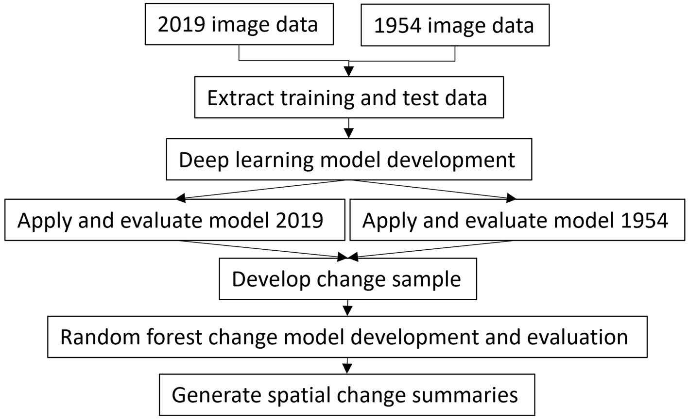
Figure 1. Overview of analysis steps.
2.2 Study site
The study site is a ~9,000 km2 area in the agricultural region of Eastern Ontario. It is located southeast of Ottawa in the Mixedwood Plains ecozone. The region is characterized by complex landscape structure, varied crop types (compositional heterogeneity), diverse land cover spatial pattern (configurational heterogeneity), presence of non-crop land cover patches including wetland, grassland and forest, and woody and herbaceous field edges. These characteristics are more evident in this region compared to other agricultural regions of Canada such as the Prairies with more homogeneous landscape structure generally related to larger field sizes.
2.3 Image data
Two sources of imagery were used in the analysis. The more recent, circa 2019, was from the Digital Raster Acquisition Project Eastern Ontario (DRAPE, acquired through Ontario GeoHub, 2019). DRAPE data was acquired in the spring of 2019/2020 (April 25th, 2019, to May 22nd, 2020) under the best cloud free, snow free, ice free, and in some cases leaf off conditions. The spatial resolution was 16 cm. Digital cameras used to acquire the data were the Vexcel UltraCam X and Vexcel UltraCam Eagle. The acquired data was orthorectified using an elevation dataset generated through image correlation. DRAPE orthorectified tiles are 1 km by 1 km and contain visible and near-infrared (NIR) bands.
The historical imagery was from 1954. These black and white air photos were and produced by Energy Mine and Resources Canada. The spatial resolution is 5.5 m. The images were scanned and georeferenced by Magda Biesiada, Data, Map, and Government Information Services, Data & GIS Services, and acquired through the Map and Data Library, University of Toronto (n.d.). Georeferencing used a spline transformation with ground control points. Visual inspection showed that results were generally quite good, but in some areas spatial misregistration with the 2019 imagery was evident. In these areas additional ground control points were collected to improve the geolocation accuracy. The root mean squared error across the study area was 3 m based on an independent random sample of 35 ground control points.
2.4 Reference data
2.4.1 Image classification
Training and test samples were extracted from a manually digitized vector map of all woody features (forest patches and LWFs) of Eastern Ontario, previously created by GLEL at Carleton University based on high resolution images (Daly, 2022; Gabriel, 2022; Hajdasz, 2023). In order to correct major differences, this dataset was overlayed on the 2019 DRAPE images. Missing or falsely included LWFs and forest patches were added or removed. Errors for labeled features were also corrected. Using these data three classes were defined as:
1. LWF: wooded hedgerows and riparian strips with a minimum length of 20 m and width less than the length similar to the definition used in Pasher et al. (2016).
2. Forest: non-linear wooded patches of various size and shape.
3. Other classes: all other land covers including crop fields, urban area, wetlands, bodies of water, etc.
Training and test data was extracted as 624 by 624 image subsets for each sample location and included the image data as the input and associated labeled raster as the training target. The spatial resolution was 32 cm, where the modified GLEL vector map was rasterized at this resolution. For the 2019 image data, it was downsampled using averaging. For the 1954 data it was upsampled using nearest neighbor to maintain the original image values and spatial structure. After initial runs the results were checked and additional training samples were added to correct errors. These additional samples were generally collected for low density forests, unique leaf-off conditions, some water bodies, urban areas, and boundaries of forests and LWFs.
Only a single image band was used as input to the model. This was done to be consistent with the 1954 imagery. For the 2019 data all bands were extracted to be used in the data augmentation during model training. This allowed the model to be trained using both the 2019 and 1954 image data providing a single model to map both periods.
Test samples (624 by 624 image subsets) were extracted for four locations in 2019 and 1954. Samples were acquired from different locations to better capture landscape variability, except for one sample area which was included to examine change potential. The spatial distribution of training and test samples are shown in Figure 2.
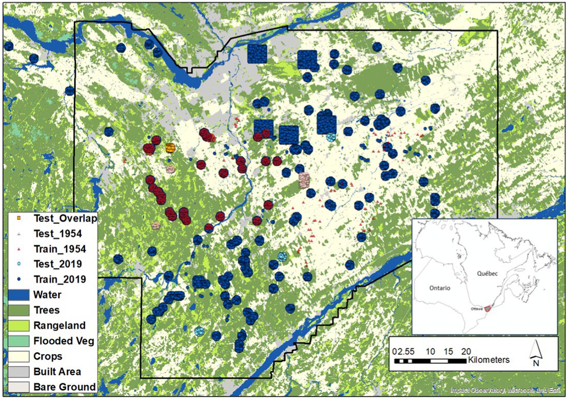
Figure 2. Train and test samples used for forest and LWF classification. The 1954 sample clusters overlap the 2019. For the test data only one area overlaps between 2019 and 1954 towards the top-left shown in orange. Background land cover is the Sentinel-2 10 m land cover time series of the world. Produced by Impact Observatory, Microsoft, and Esri.
2.4.2 Change detection
For change detection, samples were interpreted from the 2019 and 1954 image sources. Figure 3 shows the spatial distribution of the samples used for forest and LWF change. Spatially independent and randomly selected test samples were used for the change validation. These were generated by sampling gain, loss and no change objects. For each object, samples were systematically selected at approximately 20 m intervals. For LWFs, samples of no change were added along the object edges to incorporate the object boundaries.
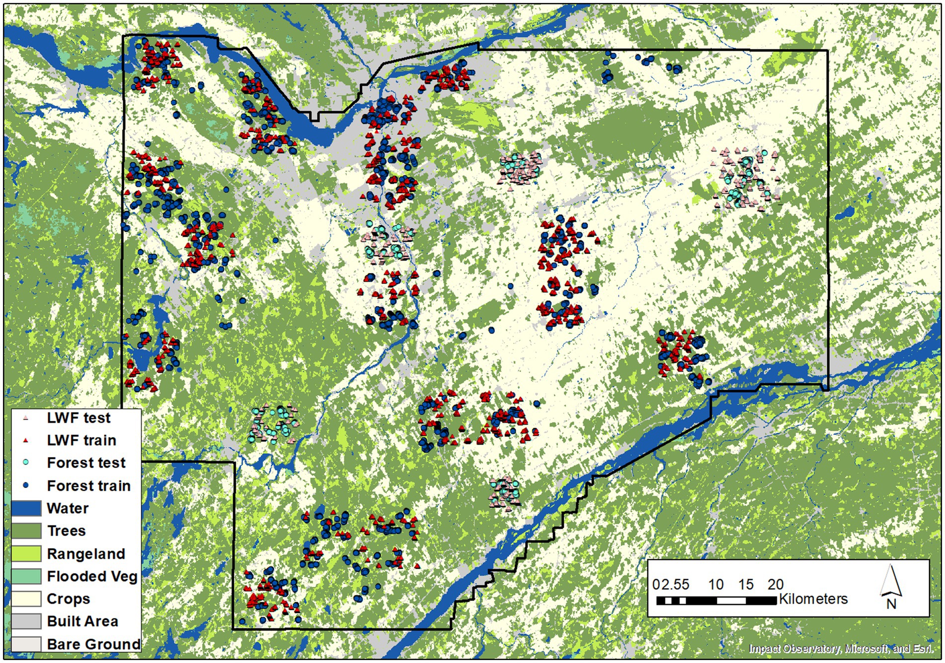
Figure 3. Train and test samples used for forest and LWF change detection. Background land cover is the Sentinel-2 10 m land cover time series of the world. Produced by Impact Observatory, Microsoft, and Esri.
2.5 Deep learning model for image classification
The U-Net architecture was used for the deep learning classification model. A U-Net in this context is known as segmentation approach, where an input image is used to predict an output segmented and labelled raster image. The specific U-Net used in this study is shown in Figure 4 with a depth of four. For the encoder part of the network residual blocks were used along with max pooling for each depth. For the decoder, spatial attention was included along with upsampling and residual blocks. Spatial attention helps the network focus on more informative spatial regions. The output of the network included softmax activation for the three classes.
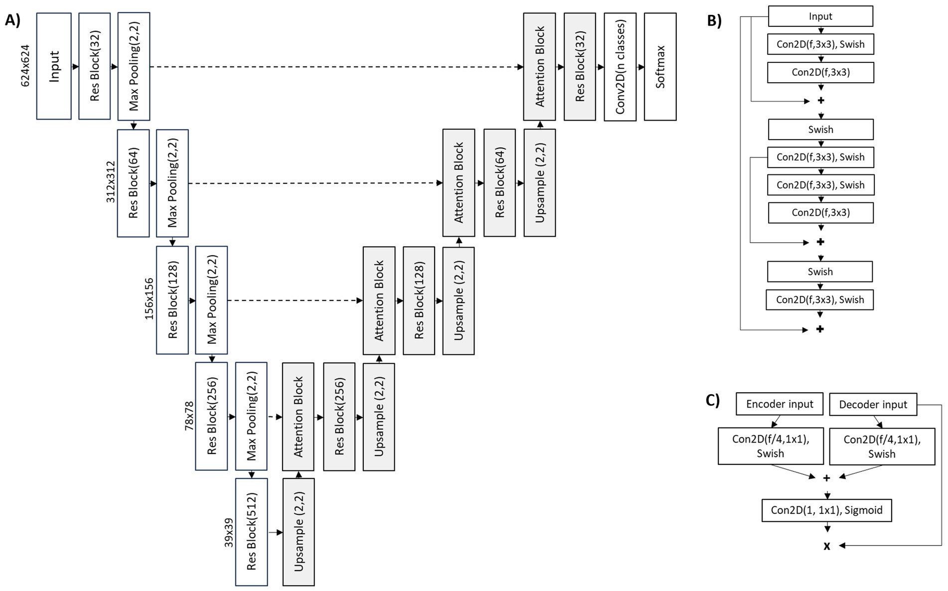
Figure 4. (A) U-Net architecture; (B) residual block; (C) attention block.
The network was implemented in Tensorflow with the Adam optimizer and learning rate set at 0.0001. Categorical focal loss was used with the focal loss set at two. This loss helps the network focus on hard to predict samples during training. Batch size was set at 5. Early stopping criteria was applied, monitoring the accuracy, where training ended if there was no improvement in 15 epochs. Standard data augmentation was applied to help the network avoid overtraining. Augmentations included random noise, bias, and flipping for the vertical and horizontal axes. To be consistent with the 1954 single band imagery, for 2019, data augmentation randomly sampled the red, green, blue or computed the average to represent a single image band in 2019.
A deep ensemble approach was used, where five U-Net models were developed with a separate random initialization for each model. Total epochs varied with each model and ranged from 70–90 epochs for the initial training. Then another 30–50 epochs with additional training data included to address errors from the initial models. The class probabilities were averaged across the five models and the standard deviation used as an indicator of prediction uncertainty.
Accuracy for LWFs was assessed at the pixel, object, and area scales using the test sample set. Forest accuracy was evaluated only at the pixel and area scales. Object-level assessment was included for LWFs to reveal detection accuracy, in contrast to the pixel-based analysis, which reflects a combination of detection and delineation accuracy. The area-based comparison was included for both LWFs and forests, as this reflects how the data are commonly applied in ecological studies.
For the pixel assessment the F1 score, precision and recall accuracy statistics were computed for each class and separately for 2019 and 1954. For the area assessment, the class area (as percent) from the samples (624 by 624 image subsets) was compared between the test data and predicted estimates. Comparison included the coefficient of determination and the mean absolute error.
The LWF object detection assessment was performed using scikit-image (van der Walt et al., 2014). Spatially distinct LWFs were identified with the connected components labeling algorithm. The skeleton of each detected LWF was computed, and its width was estimated by dividing the area by the length of its skeleton. Objects contained within 90% of the 50 pixel edges of the reference or predicted images were removed to avoid edge effects. Reference objects were considered detected if they overlapped with a prediction by at least 40%. This threshold was chosen as it represents the minimum overlap required to account for acceptable deviations in object boundaries. Reference objects with less than 40% overlap were classified as omissions (missed detections), while predicted objects with less than 40% overlap were considered commissions (false detections). A minimum length of 20 m was applied following from the LWF definition and minimum area of 15 m2. Precision, recall, and F1 scores were calculated for width thresholds ranging from 5 to 35 m, where only objects with widths less than or equal to each threshold were included.
2.6 Change detection
To detect changes, a more straightforward approach was sought, primarily motivated by efficiency and training data requirements compared to the deep learning method used for classification. The random forest classification algorithm was employed, using the results from the deep learning as input features. This approach aimed to leverage the high-quality outputs from the deep learning classification while minimizing the training and input feature requirements of the random forest model. One key advantage of random forest is its fast training and application, making it well-suited for a distributed processing approach. Alternatively, a deep learning model could have been developed directly from the imagery to detect change, but given general requirements for deep learning model development and variability in the data related to phenological timing, a much larger training sample would have likely been needed. Simple thresholding of class probability differences was also tested, but more consistent results were obtained using random forest to separate changes by incorporating uncertainty and spatial consistency.
The change analysis was performed at 1.28 m spatial resolution by average downsampling of the 32 cm forest and LWF results. This spatial resolution was selected as it did not compromise the quality of the results and reduced the output size by a factor of four. The inputs to the random forest model were the U-Net class probabilities and uncertainties for each period. For each sample this included the class probability and uncertainty for the pixel and mean of the 5 by 5, 15 by 15, and 25 by 25 local neighborhoods. Thus, for a given sample there were 16 inputs including the class probabilities plus uncertainties for a pixel for each time period and the local neighborhoods. The number of trees used was 100 and all other parameters were set as default. Results of the change analysis were filtered to remove change objects smaller than 49 m2. Change classes included gain, loss, or no change for forests or LWFs. F1, precision, and recall statistics were computed to assess accuracy. To better visualize and summarize the results, net change was computed for a 1 km grid across the study area.
3 Results
3.1 Forest and LWF classification
Example results for the forest and LWF classification in each period are shown in Figure 5 for a large spatial extent. These results show good agreement in terms of the general pattern detected as forest or LWF in both periods.
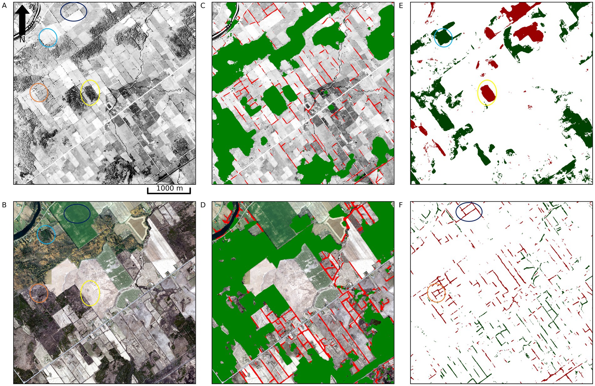
Figure 5. Example results for a 4 km extent. (A) 1954 image; (B) 2019 image; (C) 1954 forest and LWF classification results (red = LWF, green = forest); (D) 2019 forest and LWF classification results (red = LWF, green = forest); (E) Forest change results (dark red = loss, dark green = gain); (F) LWF change results (dark red = loss, dark green = gain). Circles indicate different changes: yellow—forest loss; light blue—forest gain; dark blue—LWF loss; orange—LWF loss to forest gain.
Example results for a more detailed, zoomed-in extent are presented in Figure 6. It reveals that the forests and LWFs were well detected, but that the LWF predictions tend to be larger than the reference in some cases. The reference data is not a prefect delineation of the LWF and is often larger and has a generalized shape compared to what is evident from the image. This error in the training data was the primary reason for the LWF prediction errors. Refinement of the LWF objects in the GLEL dataset was not undertaken as it would have been a significant effort. Only missing objects or false objects were corrected in the training data used.
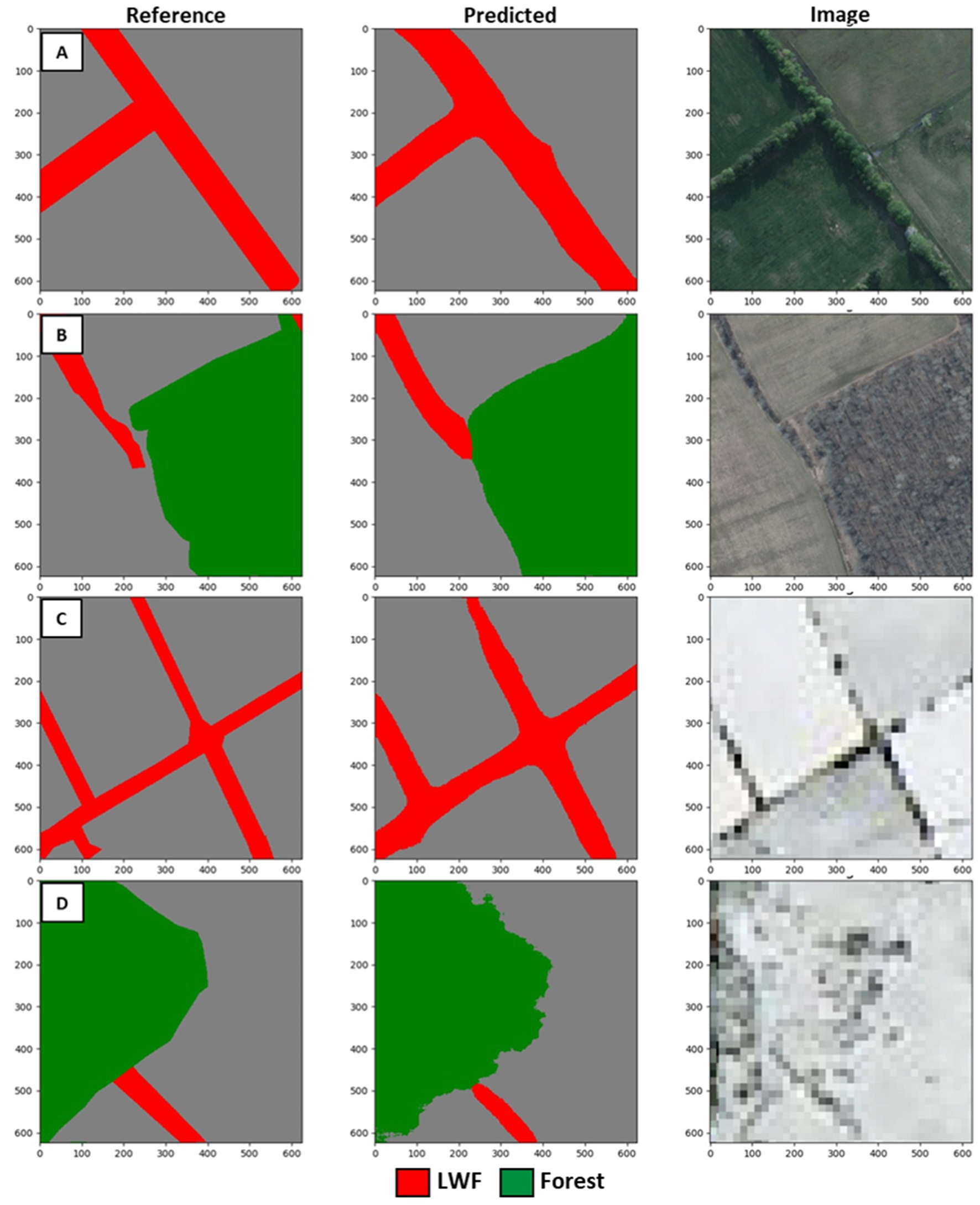
Figure 6. Example prediction results for (A,B) 2019; (C,D) 1954.
Error matrices and accuracy statistics for each class are given in Table 1 for 1954 and 2019 based on the test data. The forest and other classes have very high accuracy 90% or higher for both periods based on the F1 score. LWF accuracy is lower and is 70% in 2019 and 66% in 1954. This is partially attributable to limitations in LWF delineation accuracy in both the predicted and reference data, where narrow linear features, shape complexity, and intersections coupled with the generalized nature of the reference data and geolocation error introduces ambiguity in object boundaries and reduces delineation precision. However, as can be seen in in Figures 5, 6, LWF detection accuracy is good. That is LWFs are well detected, but differences in the exact shape between the reference and predicted LWF objects are evident.
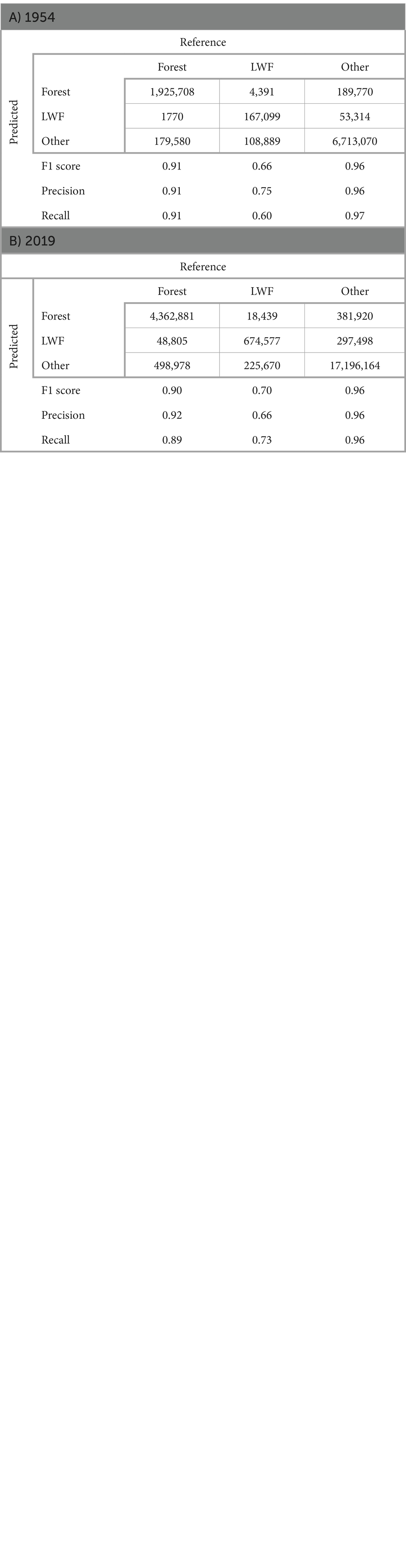
Table 1. Error matrix and accuracy statistics for A) 1954 and B) 2019 test samples.
Figure 7 shows the results of the LWF object detection analysis for the different width thresholds for 2019 and 1954. Few objects were detected for widths less than or equal to 5 m and these results are not reliable. For the 10 m threshold, the F1 score is ~50%, but in terms of the total area this was less than 4% of the sample. For the 15 m threshold, the F1 score approaches 70% and for all data was 77%. This supports the visual conclusion of good detection accuracy. The 2019 results (F1 score = 83%) are better than 1954 (F1 score = 73%) as expected due to the lower image quality for 1954.
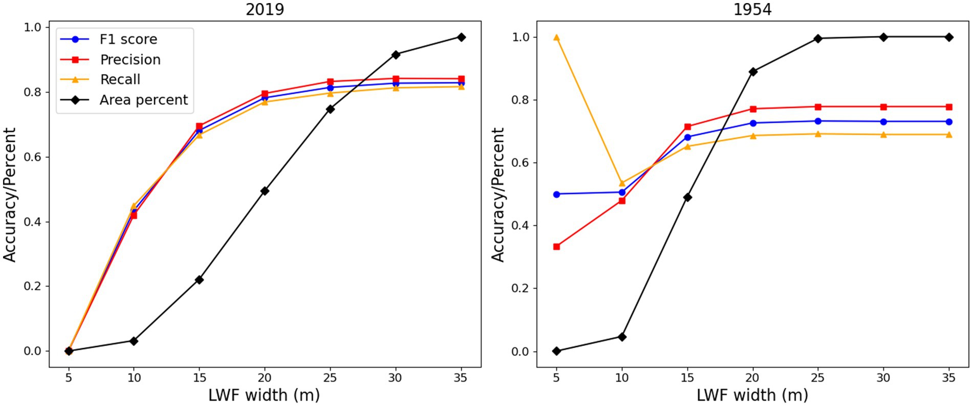
Figure 7. LWF object accuracy for width thresholds. At each threshold objects with widths less than or equal to the threshold were included.
For the area-based assessment, results indicate strong correlation and low mean absolute errors supporting again strong detection accuracy and averaging out of delineation errors in particular for the LWFs (Figure 8). The mean absolute error for forests was 2.73 and 1.26% for LWFs. The range of forest area was greater in the sample with a relatively equal distribution from 0 to 100%. For LWFs the majority of the data was less than 30%.
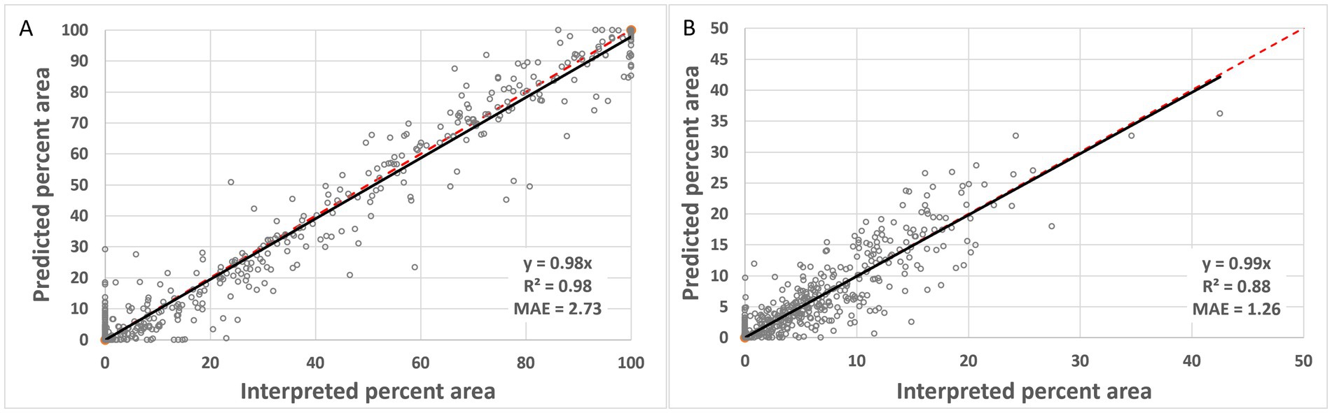
Figure 8. Comparison of predicted and reference data as percent area (pooled 200 by 200 m extents for 2019 and 1954) for (A) forests and (B) LWFs. Black line is the regression line and the red dashed represents the 1:1 line.
3.2 Forest and LWF change
Example results for the change between 2019 and 1954 are shown in Figure 5 for a large extent highlighting areas of gain and loss. At this scale changes appear well captured. Change accuracy based on the spatial holdout are given Table 2 and show that the accuracies were all above 81%. Careful visual examination of the results confirmed high accuracy, except for ambiguous areas related to lower density forest in the lower quality 1954 imagery or sparsely treed LWFs and wetlands. Low density forest wetlands were more ambiguous in the 1954 imagery in particular. Urban areas were also sometimes captured as forest loss, because these areas were not well trained in the 1954 imagery and were falsely identified as forest. However, in the 2019 imagery urban areas were well trained and not identified as forest. For this reason, all urban areas were checked and corrected in the final results. Change objects were often well detected, but boundaries were in some instances over or underestimated.
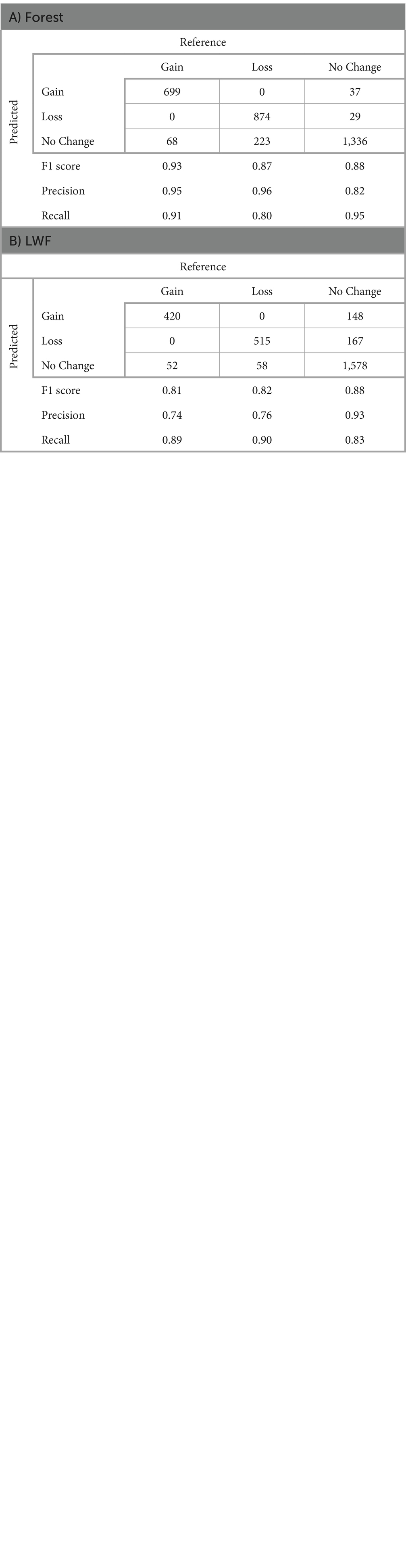
Table 2. Error matrix and accuracy statistics for change detection.
Figures 9, 10 show the net change and mean class probabilities from 1954 to 2019 for a 1 km grid. Forest area has increased in the region by 12.3% and decreased by 3.8% resulting in a net gain of forest of 8.5%. The gain in forest largely occurred in previous agricultural fields. Decreases occur more locally and for a smaller magnitude related to agriculture, urban development, or conversion to wetland conditions. LWF change was more balanced, increasing by 1.55% and decreasing by 2.08% for a net loss of 0.53%. Loss in LWFs occurred mostly in areas of forest gain. Some loss was also due to urban development. Removing LWF loss due to forest gain, the net change in LWFs showed a small gain of 0.15% suggesting that LWFs have been stable in the region.
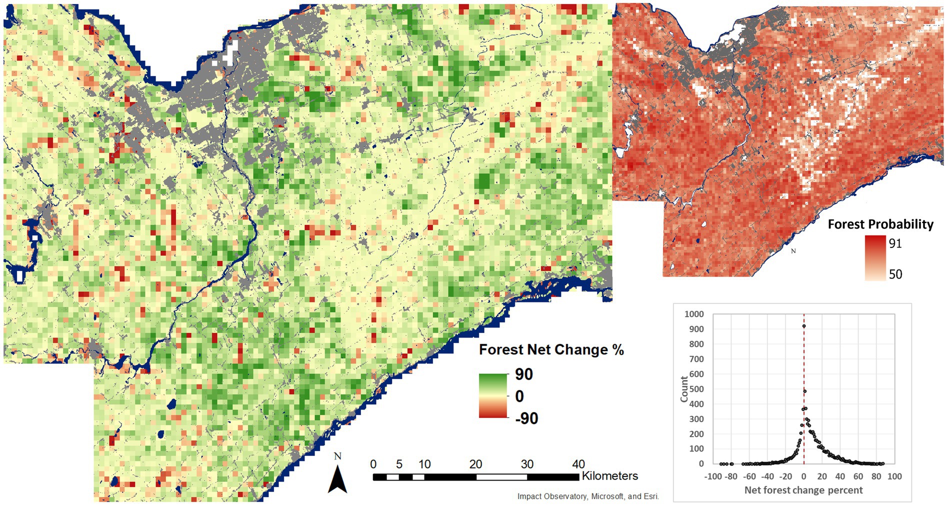
Figure 9. Net change in forest area per 1 km grid cell across the study area (left), and mean forest probability from 2019 and 1954 U-Net model outputs (right). Grid cells with less than 1% forest cover have been set as no data in the mean forest probability layer. Water and built-up areas are from the Sentinel-2 10 m land cover time series of the world. Produced by Impact Observatory, Microsoft, and Esri.
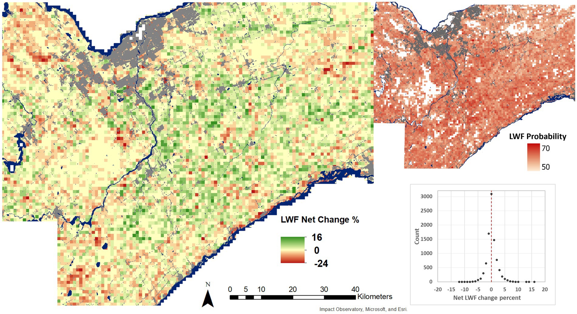
Figure 10. Net change in LWF area per 1 km grid cell across the study area (left), and mean LWF probability from 2019 and 1954 U-Net model outputs (right). Grid cells with less than 1% LWF cover have been set as no data in the mean LWF probability layer. Water and built-up areas are from the Sentinel-2 10 m land cover time series of the world. Produced by Impact Observatory, Microsoft, and Esri.
4 Discussion
The ability to accurately map and assess changes in forests and LWFs is critical for evaluating biodiversity and other ecosystem services such as carbon storage. This study demonstrates the capability to map forests and LWFs using spatially and spectrally heterogeneous high-spatial resolution image datasets. The deep learning model developed here was effective utilizing a single image band to consistently map forests and LWFs over the period from 1954 to 2019. Outputs from the model were subsequently employed to assess changes across the study area. Accuracy of the change results were largely constrained by the quality of the 1954 image data. While the incorporation of higher-quality historical imagery with additional spectral content could potentially improve the accuracy of the findings, it would reduce the temporal extent of the analysis. The primary objective of examining changes over the longest possible period was to better understand how biodiversity and ecosystem services in the region have been influenced by shifts in forest and LWF distributions.
Another challenge in this analysis was the use of early spring imagery with various degrees of leaf development conditions in 2019. This increased the variability for which the deep learning model was required to account for and led to errors in some cases. Much of this error was addressed through collection of additional training samples to improve the model. However, with a more consistent image data source, reduced training data and more accurate results are possible.
Geolocation quality is a crucial factor in change analysis. Improving geolocation accuracy would enhance results, particularly for LWFs, which are narrow objects and prone to misalignment. Significant effort was made to refine geolocation accuracy to enable change detection at the pixel scale. The object and area-based analysis were incorporated to minimize geolocation error on the results. In the object-based approach, the overlap criteria were applied to account for minor misalignments, ensuring that slight shifts did not falsely indicate change in addition to accounting for boundary errors. In the area-based assessment, a misaligned LWF is not counted as a change, as the total area remains consistent despite positional inaccuracies. However, there could be some potential error along the boundaries of the sampled area (624 by 624 pixels in this study), which would depend on factors such as the spatial configuration, the occurrence of LWFs near edges, and the size of the area being analyzed. Additionally, to evaluate changes in spatial configuration, such as local connectivity, an area-based approach is inherently required.
In addition to improving image data, enhancing the quality of training data is expected to improve the delineation of both forests and more importantly LWFs. The accuracy of the delineation can be influenced by several factors, including the scale at which the delineation is made, image properties like sensor-viewing geometry, and the skill of the interpreter among others. For large-extent production efforts, such as the GLEL initiative, a balance between accuracy and efficiency is required. Ultimately, refining and adjusting the interpretations to the source image would improve the results. In this analysis, the model’s tendency to delineate LWFs slightly wider than the reference data introduced a small bias. Fortunately, this bias was fairly consistent between 1954 and 2019, so it is not expected to significantly affect the change results. Additionally, the training data for change detection included edge samples specifically chosen to help account for potential bias.
From this analysis between 1954 and 2019 there has been a reduction in the agriculture area and associated increase in forests in this region. As a generalized guideline Arroyo-Rodrıguez et al. (2020, 2021) recommend that 40% forest cover be maintained to support biodiversity. Forest area in 2019 was 36%, including the area of LWFs this increases to 39% very close to this recommendation. However, analysis for the period beginning around the late 2000s, indicates a reversal of this trend, with forest cover declining across the region (Mesman, 2016; Fyson et al., 2024).
Although LWFs declined slightly due to forest gains, forests may offer greater biodiversity benefits (Slade et al., 2013). However, a global meta-analysis by García de León et al. (2021) found no significant increase in biodiversity in forests compared to LWFs, though ecosystem services were enhanced. Not considering areas of forest gain, a very small increase in LWFs was observed. In the central region that was mostly agriculture cover in 2019 and 1954 shows a general increase in LWFs (Figure 2 crop area and Figure 10 LWF change). This increase is likely to have a positive effect on bird biodiversity (Wilson et al., 2017; de Zwaan et al., 2024). However, other factors, not examined, affecting biodiversity in the region such as urban expansion and larger field sizes are expected to negatively impact biodiversity. Since the 1950s, industrial development and urban expansion resulting from various industries including manufacturing, education, and technology have been important drivers of change. Agriculture has remained a key component of the regional economy since 1954 (Minnes and Douglas, 2013). Although the total area of cropped land in Eastern Ontario has remained relatively stable over the past few decades (Smith, 2015; Caldwell et al., 2022), farming practices have shifted. There has been a move away from low-intensity perennial crops, such as hay and pasture, toward more intensive annual crops like corn, soybeans, and wheat. Additionally, average field sizes have increased due to the consolidation of adjacent fields and the removal of LWFs (Smith, 2015; Ontario’s Agricultural Soil Health and Conservation Strategy Report, 2022). Visual inspection of the image data used here suggests that field sizes have increased from 1954 to 2019, leading to a reduction in field margins of different types including LWFs, which are important for supporting biodiversity across various taxonomic groups (Fahrig et al., 2015). Additionally, field sizes and LWFs have been shown to affect the availability of milkweed, which is vital for supporting monarch butterflies (Martin et al., 2021).
Future work will focus on improving accuracy, incorporating additional time periods, extending to additional study areas, and expanding the characterization of linear features to include non-woody field margins. Additionally, wetlands and urban areas need to be considered, as both have undergone significant change in the region. These improvements are crucial for gaining a deeper understanding of the current state and the changes impacting biodiversity and carbon storage in the region, which is essential for supporting policies that effectively balance economic with conservation objectives.
Data availability statement
Publicly available data were analyzed in this study. This data can be found via the following links: https://geohub.lio.gov.on.ca/datasets/lio::digital-raster-acquisition-project-eastern-ontario-drape-2019-2020-stereo-index/explore?location=45.150450%2C-76.439692%2C7.75 and https://mdl.library.utoronto.ca/collections/air-photos/1954-air-photos-southern-ontario/index.
Author contributions
DP: Conceptualization, Formal analysis, Methodology, Project administration, Software, Writing – original draft, Writing – review & editing. NA: Conceptualization, Data curation, Methodology, Writing – original draft, Writing – review & editing. MM: Data curation, Methodology, Software, Writing – review & editing. JP: Conceptualization, Funding acquisition, Project administration, Writing – review & editing. JD: Conceptualization, Funding acquisition, Project administration, Writing – review & editing.
Funding
The author(s) declare that no financial support was received for the research and/or publication of this article.
Acknowledgments
We would like to express our gratitude to David Lapen and the Environmental OneHealth Observatory (ECO2) team in Agriculture and Agrifood Canada for the support during this research. We greatly appreciate Patrick Kirby’s assistance in preparing the image datasets and Ash Nassef’s support in developing the training samples. We also would like to acknowledge Carleton University GIS Library and Meghan Kenny for packaging and providing the DRAPE 2019 image data. Generative AI (GPT-4o) was used to suggest edits to select paragraphs in the introduction and discussion sections of the manuscript.
Conflict of interest
The authors declare that the research was conducted in the absence of any commercial or financial relationships that could be construed as a potential conflict of interest.
Generative AI statement
The author(s) declare that Gen AI was used in the creation of this manuscript.
Publisher’s note
All claims expressed in this article are solely those of the authors and do not necessarily represent those of their affiliated organizations, or those of the publisher, the editors and the reviewers. Any product that may be evaluated in this article, or claim that may be made by its manufacturer, is not guaranteed or endorsed by the publisher.
References
Adegun, A. A., Viriri, S., and Tapamo, J. R. (2023). Review of deep learning methods for remote sensing satellite images classification: experimental survey and comparative analysis. J. Big Data 10:93. doi: 10.1186/s40537-023-00772-x
Ahlswede, S., Asam, S., and Röder, A. (2021). Hedgerow object detection in very high-resolution satellite images using convolutional neural networks. J. Appl. Remote. Sens. 15, 1–28. doi: 10.1117/1.jrs.15.018501
Aksoy, S., Akçay, H. G., and Wassenaar, T. (2010). Automatic mapping of linear woody vegetation features in agricultural landscapes using very high resolution imagery. IEEE Trans. Geosci. Remote Sens. 48, 511–522. doi: 10.1109/TGRS.2009.2027702
Álvarez, F. A., Gomez-Mediavilla, G., López-Estébanez, N., and Holgado, P. M. (2021). Classification of Mediterranean hedgerows: a methodological approximation. MethodsX 8:101355. doi: 10.1016/j.mex.2021.101355
Arroyo-Rodrıguez, V., Fahrig, L., Tabarelli, M., Watling, J. I., Tischendorf, L., Benchimol, M., et al. (2020). Designing optimal human-modified landscapes for forest biodiversity conservation. Ecol. Lett. 23, 1404–1420. doi: 10.1111/ele.13535
Arroyo-Rodríguez, V., Fahrig, L., Watling, J. I., Nowakowski, J., Tabarelli, M., Tischendorf, L., et al. (2021). Preserving 40% forest cover is a valuable and well-supported conservation guideline: reply to Banks-Leite et al. Ecol. Lett. 24, 1114–1116. doi: 10.1111/ele.13689
Aviron, S., Lalechère, E., Duflot, R., Parisey, N., and Poggi, S. (2018). Connectivity of cropped vs. semi-natural habitats mediates biodiversity: a case study of carabid beetles communities. Agric. Ecosyst. Environ. 268, 34–43. doi: 10.1016/j.agee.2018.08.025
Axe, M. S., Grange, I. D., and Conway, J. S. (2017). Carbon storage in hedge biomass—A case study of actively managed hedges in England. Agric. Ecosyst. Environ. 250, 81–88. doi: 10.1016/j.agee.2017.08.008
Benhamou, C., Salmon-Monviola, J., Durand, P., Grimaldi, C., and Merot, P. (2013). Modeling the interaction between fields and a surrounding hedgerow network and its impact on water and nitrogen flows of a small watershed. Agric. Water Manag. 121, 62–72. doi: 10.1016/j.agwat.2013.01.004
Betbeder, J., Nabucet, J., Pottier, E., Baudry, J., Corgne, S., and Hubert-Moy, L. (2014). Detection and characterization of hedgerows using Terra SAR-X imagery. Remote Sens. 6, 3752–3769. doi: 10.3390/rs6053752
Biffi, S., Chapman, P. J., Grayson, R. P., and Ziv, G. (2022). Soil carbon sequestration potential of planting hedgerows in agricultural landscapes. J. Environ. Manag. 307:114484. doi: 10.1016/j.jenvman.2022.114484
Bishop, G. A., Fijen, T. P. M., Desposato, B. N., Scheper, J., and Kleijn, D. (2023). Hedgerows have contrasting effects on pollinators and natural enemies and limited spillover effects on apple production. Agric. Ecosyst. Environ. 346:108364. doi: 10.1016/j.agee.2023.108364
Boinot, S., Alignier, A., Pétillon, J., Ridel, A., and Aviron, S. (2023). Hedgerows are more multifunctional in preserved bocage landscapes. Ecol. Indic. 154:110689. doi: 10.1016/j.ecolind.2023.110689
Caldwell, W., Epp, S., Wan, X., Singer, R., Drake, E., and Sousa, E. C. (2022). Farmland preservation and urban expansion: case study of southern Ontario, Canada. Front. Sustain. Food Syst. 6:777816. doi: 10.3389/fsufs.2022.777816
Cao, K., and Zhang, X. (2020). An improved Res-UNet model for tree species classification using airborne high-resolution images. Remote Sens. 12:1128. doi: 10.3390/rs12071128
Clausen, M. A., Elle, E., and Smukler, S. M. (2022). Evaluating hedgerows for wild bee conservation in intensively managed agricultural landscapes. Agric. Ecosyst. Environ. 326:107814. doi: 10.1016/j.agee.2021.107814
Collier, M. J. (2021). Are field boundary hedgerows the earliest example of a nature-based solution? Environ Sci Policy 120, 73–80. doi: 10.1016/j.envsci.2021.02.008
Dadam, D., and Siriwardena, G. M. (2019). Agri-environment effects on birds in Wales: Tir Gofal benefited woodland and hedgerow species. Agric. Ecosyst. Environ. 284:106587. doi: 10.1016/j.agee.2019.106587
Daly, L. J. (2022). “The Independent Effects of Forest Amount, Fragmentation and Structural Connectivity on Small Mammals’ Diversity, Abundance and Occurrence.” Doctoral diss., Carleton University.
de Zwaan, D. R., Alavi, N., Mitchell, G. W., Lapen, D. R., Duffe, J., and Wilson, S. (2022). Balancing conservation priorities for grassland and forest specialist bird communities in agriculturally dominated landscapes. Biol. Conserv. 265:109402. doi: 10.1016/j.biocon.2021.109402
de Zwaan, D. R., Hannah, K. C., Alavi, N., Mitchell, G. W., Lapen, D. R., Duffe, J., et al. (2024). Local and regional-scale effects of hedgerows on grassland-and forest-associated bird populations within agroecosystems. Ecol. Appl. 34, e2959–e2916. doi: 10.1002/eap.2959
Dondina, O., Kataoka, L., Orioli, V., and Bani, L. (2016). How to manage hedgerows as effective ecological corridors for mammals: A two-species approach. Agric. Ecosyst. Environ. 231, 283–290. doi: 10.1016/j.agee.2016.07.005
Dowell, L. (2020). Evaluating hedgerow and riparian buffer carbon storage potential in the Lower Fraser Valley from a field-and landscape-level perspective (T). University of British Columbia. Available online at: https://open.library.ubc.ca/collections/ubctheses/24/items/1.0395372
EU, CLMS, EEA. (2021). Small Woody Features 2018 and Small Woody Features Changes 2015–2018. Product user manual.
Fahrig, L., Girard, J., Duro, D., Pasher, J., Smith, A., Javorek, S., et al. (2015). Farmlands with smaller crop fields have higher within-field biodiversity. Agric. Ecosyst. Environ. 200, 219–234. doi: 10.1016/j.agee.2014.11.018
Fyson, V. K., Wilmshurst, J. F., and Callaghan, C. (2024). The changing agricultural landscape in Canada’s Mixedwood Plains Ecozone (2011–2022) and the implications for biodiversity. Facets 9, 1–11. doi: 10.1139/facets-2024-0019
Gabriel, J. (2022). “The Independent Effects of Forest Amount, Fragmentation, and Corridors on Forest Understory Plant Diversity.” Doctoral diss., Carleton University.
García de León, D., Rey Benayas, J. M., and Andivia, E. (2021). Contributions of hedgerows to people: a global meta-analysis. Front. Conserv. Sci. 2:789612. doi: 10.3389/fcosc.2021.789612
Garratt, M. P. D., Senapathi, D., Coston, D. J., Mortimer, S. R., and Potts, S. G. (2017). The benefits of hedgerows for pollinators and natural enemies depends on hedge quality and landscape context. Agric. Ecosyst. Environ. 247, 363–370. doi: 10.1016/j.agee.2017.06.048
Hajdasz, A. C. (2023). “Forest Amount, Not Fragmentation or Connectivity, Increases Bird Species Richness.” Doctoral diss., Carleton University.
Heath, S. K., Soykan, C. U., Velas, K. L., Kelsey, R., and Kross, S. M. (2017). A bustle in the hedgerow: Woody field margins boost on farm avian diversity and abundance in an intensive agricultural landscape. Biol. Conserv. 212, 153–161. doi: 10.1016/j.biocon.2017.05.031
Lacoeuilhe, A., Machon, N., Julien, J. F., and Kerbiriou, C. (2016). Effects of hedgerows on bats and bush crickets at different spatial scales. Acta Oecol. 71, 61–72. doi: 10.1016/j.actao.2016.01.009
Lecq, S., Loisel, A., Brischoux, F., Mullin, S. J., and Bonnet, X. (2017). Importance of ground refuges for the biodiversity in agricultural hedgerows. Ecol. Indic. 72, 615–626. doi: 10.1016/j.ecolind.2016.08.032
Lecq, S., Loisel, A., Mullin, S. J., and Bonnet, X. (2018). Manipulating hedgerow quality: Embankment size influences animal biodiversity in a peri-urban context. Urban For. Urban Green. 35, 1–7. doi: 10.1016/j.ufug.2018.08.002
Liu, P., Wang, C., Ye, M., and Han, R. (2024). Coastal zone classification based on U-Net and remote sensing. Appl. Sci. (Switzerland) 14:7050. doi: 10.3390/app14167050
Long, R. F., Garbach, K., and Morandin, L. A. (2017). Hedgerow benefits align with food production and sustainability goals. Calif. Agric. 71, 117–119. doi: 10.3733/ca.2017a0020
Lucas, C., Bouten, W., Koma, Z., Kissling, W. D., and Seijmonsbergen, A. C. (2019). Identification of linear vegetation elements in a rural landscape using LiDAR point clouds. Remote Sens. 11:292. doi: 10.3390/rs11030292
Ludwig, M., Schlinkert, H., Holzschuh, A., Fischer, C., Scherber, C., Trnka, A., et al. (2012). Landscape-moderated bird nest predation in hedges and forest edges. Acta Oecol. 45, 50–56. doi: 10.1016/j.actao.2012.08.008
Map and Data Library, University of Toronto (n.d.) Available online at: https://mdl.library.utoronto.ca/collections/air-photos/1954-air-photos-southern-ontario/index (Accessed March 2024)
Martin, A. E., Mitchell, G. W., Girard, J. M., and Fahrig, L. (2021). More milkweed in farmlands containing small, annual crop fields and many hedgerows. Agric. Ecosyst. Environ. 319:107567. doi: 10.1016/j.agee.2021.107567
Maskell, L. C., Norton, L. R., Carey, P. D., Wood, J., Bunce, C. M., and Barr, R. G. H. (2008). CS Technical Report No 1/07: Field Mapping Handbook v1.0 Field Mapping Handbook: Field Mapping Handbook v1.0 2 Contents.
McCann, T., Cooper, A., Rogers, D., McKenzie, P., and McErlean, T. (2017). How hedge woody species diversity and habitat change is a function of land use history and recent management in a European agricultural landscape. J. Environ. Manag. 196, 692–701. doi: 10.1016/j.jenvman.2017.03.066
Minnes, S., and Douglas, D. J. A. (2013). A profile of eastern Ontario. Canadian Regional Development. School of Environmental Design and Rural Development University of Guelph
Morandin, L. A., Long, R. F., and Kremen, C. (2014). Hedgerows enhance beneficial insects on adjacent tomato fields in an intensive agricultural landscape. Agric. Ecosyst. Environ. 189, 164–170. doi: 10.1016/j.agee.2014.03.030
Morelli, F. (2013). Relative importance of marginal vegetation (shrubs, hedgerows, isolated trees) surrogate of HNV farmland for bird species distribution in Central Italy. Ecol. Eng. 57, 261–266. doi: 10.1016/j.ecoleng.2013.04.043
Muro, J., Blickensdörfer, L., Don, A., Köber, A., Schwieder, M., and Erasmi, S. (2024). Remote Sensing of Environment Hedgerow mapping with high resolution satellite imagery to support policy initiatives at national level. Available online at: https://ssrn.com/abstract=5011709
Ontario GeoHub (2019). Available online at: https://geohub.lio.gov.on.ca/datasets/lio::digital-raster-acquisition-project-eastern-ontario-drape-2019-2020-1km-index/about (Accessed May 2020)
Ontario’s Agricultural Soil Health and Conservation Strategy Report. (2022). Available online at: https://www.ontario.ca/page/new-horizons-ontarios-agricultural-soil-health-and-conservation-strategy (Accessed April 2025)
Pasher, J., McGovern, M., and Putinski, V. (2016). Measuring and monitoring linear woody features in agricultural landscapes through earth observation data as an indicator of habitat availability. Int. J. Appl. Earth Obs. Geoinf. 44, 113–123. doi: 10.1016/j.jag.2015.07.008
Pirbasti, M. A., Mcardle, G., and Akbari, V. (2024). Hedgerows monitoring in remote sensing: a comprehensive review. In IEEE Access. Institute of Electrical and Electronics Engineers Inc. doi: 10.1109/ACCESS.2024.3485512
Ronneberger, O., Fischer, P., and Brox, T. (2015). U-Net: Convolutional networks for biomedical image segmentation. Lecture Notes in Computer Science (Including Subseries Lecture Notes in Artificial Intelligence and Lecture Notes in Bioinformatics), 9351, 234–241. doi: 10.1007/978-3-319-24574-4_28
Singh, G., Singh, S., Sethi, G., and Sood, V. (2022). Deep learning in the mapping of agricultural land use using Sentinel-2 Satellite Data. Aust. Geogr. 2, 691–700. doi: 10.3390/geographies2040042
Slade, E. M., Merckx, T., Riutta, T., Bebber, D. P., Redhead, D., Riordan, P., et al. (2013). Life-history traits and landscape characteristics predict macro-moth responses to forest fragmentation. Ecology 94, 1519–1530. doi: 10.1890/12-1366.1
Smigaj, M., and Gaulton, R. (2021). Capturing hedgerow structure and flowering abundance with UAV remote sensing. Remote Sens. Ecol. Conserv 7, 521–533. doi: 10.1002/rse2.208
Smith, P. (2015). Long-term temporal trends in agri-environment and agricultural land use in Ontario, Canada: transformation, transition and significance. J. Geogr. Geol. 7:32. doi: 10.5539/jgg.v7n2p32
Solórzano, J. V., Mas, J. F., Gao, Y., and Gallardo-Cruz, J. A. (2021). Land use land cover classification with U-net: Advantages of combining sentinel-1 and sentinel-2 imagery. Remote Sens. 13:3600. doi: 10.3390/rs13183600
Staley, J. T., Sparks, T. H., Croxton, P. J., Baldock, K. C. R., Heard, M. S., Hulmes, S., et al. (2012). Long-term effects of hedgerow management policies on resource provision for wildlife. Biol. Conserv. 145, 24–29. doi: 10.1016/j.biocon.2011.09.006
Staley, J. T., Wolton, R., and Norton, L. R. (2023). Improving and expanding hedgerows—recommendations for a semi-natural habitat in agricultural landscapes. Ecol. Solut. Evid. 4, 1–7. doi: 10.1002/2688-8319.12209
Statistics Canada (2021) Available online at: https://www150.statcan.gc.ca/n1/pub/16-001-m/16-001-m2023001-eng.htm (Accessed November 2024)
Sullivan, M. J. P., Pearce-Higgins, J. W., Newson, S. E., Scholefield, P., Brereton, T., and Oliver, T. H. (2017). A national-scale model of linear features improves predictions of farmland biodiversity. J. Appl. Ecol. 54, 1776–1784. doi: 10.1111/1365-2664.12912
Sybertz, J., Matthies, S., Schaarschmidt, F., Reich, M., and von Haaren, C. (2017). Assessing the value of field margins for butterflies and plants: how to document and enhance biodiversity at the farm scale. Agric. Ecosyst. Environ. 249, 165–176. doi: 10.1016/j.agee.2017.08.018
Tansey, K., Chambers, I., Anstee, A., Denniss, A., and Lamb, A. (2009). Object-oriented classification of very high resolution airborne imagery for the extraction of hedgerows and field margin cover in agricultural areas. Appl. Geogr. 29, 145–157. doi: 10.1016/j.apgeog.2008.08.004
Thompson, J. B., Symonds, J., Carlisle, L., Iles, A., Karp, D. S., Ory, J., et al. (2023). Remote sensing of hedgerows, windbreaks, and winter cover crops in California’s Central Coast reveals low adoption but hotspots of use. Front. Sustain. Food Syst. 7:1052029. doi: 10.3389/fsufs.2023.1052029
Tschumi, M., Birkhofer, K., Blasiusson, S., Jörgensen, M., Smith, H. G., and Ekroos, J. (2020). Woody elements benefit bird diversity to a larger extent than semi-natural grasslands in cereal-dominated landscapes. Basic Appl. Ecol. 46, 15–23. doi: 10.1016/j.baae.2020.03.005
Vallé, C., le Viol, I., Kerbiriou, C., Bas, Y., Jiguet, F., and Princé, K. (2023). Farmland biodiversity benefits from small woody features. Biol. Conserv. 286:110262. doi: 10.1016/j.biocon.2023.110262
van der Walt, S., Schönberger, J. L., Nunez-Iglesias, J., Boulogne, F., Warner, J. D., Yager, N., et al. (2014). Scikit-image: image processing in python. PeerJ 2:e453. doi: 10.7717/peerj.453
Vannier, C., and Hubert-Moy, L. (2014). Multiscale comparison of remote-sensing data for linear woody vegetation mapping. Int. J. Remote Sens. 35, 7376–7399. doi: 10.1080/01431161.2014.968683
Warren, M., Wilson, S., Alavi, N., Duffe, J., Lapen, D., and Mitchell, G. W., (in press), Bats respond positively to local hedgerow structure and forest amount at a landscape scale in a North American agroecosystem.
Wilson, S., Alavi, N., Pouliot, D., and Mitchell, G. W. (2020). Similarity between agricultural and natural land covers shapes how biodiversity responds to agricultural expansion at landscape scales. Agric. Ecosyst. Environ. 301:107052. doi: 10.1016/j.agee.2020.107052
Keywords: linear woody features, hedgerows, forest, remote sensing, change detection, biodiversity, agriculture
Citation: Pouliot D, Alavi N, Mao M, Pasher J and Duffe J (2025) Detecting forest and linear woody feature change between 1954 and 2019 in Southeastern Canadian agroecosystems for regional biodiversity assessment. Front. Sustain. Food Syst. 9:1581252. doi: 10.3389/fsufs.2025.1581252
Edited by:
Sawaid Abbas, University of the Punjab, PakistanReviewed by:
Halil Ibrahim Senol, Harran University, TürkiyeXingjing Chen, Institute of Forest Resource Information Techniques, Chinese Academy of Forestry, China
Copyright © 2025 Pouliot, Alavi, Mao, Pasher and Duffe. This is an open-access article distributed under the terms of the Creative Commons Attribution License (CC BY). The use, distribution or reproduction in other forums is permitted, provided the original author(s) and the copyright owner(s) are credited and that the original publication in this journal is cited, in accordance with accepted academic practice. No use, distribution or reproduction is permitted which does not comply with these terms.
*Correspondence: Darren Pouliot, RGFycmVuLlBvdWxpb3RAZWMuZ2MuY2E=