Enhancing AquaCrop model precision for accurate simulation of sweet potato and taro landraces

Neglected and underutilised crop species (NUS) such as orange-fleshed sweet potato (OFSP) and taro are nutrient-dense, climate-resilient crops with high potential to diversify food systems. While the AquaCrop model has been calibrated to simulate canopy cover (CC), biomass, and yield for both crops, independent testing across diverse agro-ecological zones is required to critically assess model robustness. We, therefore, evaluated AquaCrop’s ability to simulate the growth and yield of OFSP and taro at three locations in the KwaZulu-Natal province, South Africa. Critical recalibration adjustments included reducing taro’s maximum rooting depth, modifying soil water depletion thresholds to better reflect water stress, and parameterising phenology based on tuber mass stabilisation. Recalibration improved model performance for CC (R², coefficient of determination, up to 0.954 for OFSP; 0.632 for taro), biomass (NSE, Nash-Sutcliffe efficiency, up to 0.975), and final yield (absolute deviations ≤ 6% under optimal irrigation). Validation across three locations confirmed that AquaCrop reliably simulates growth and yield under non-stressed conditions, although performance declined under water-limited environments. The model was run in growing degree-day mode to account for climate variability, which is recommended for future validations. These results demonstrate that, with high-quality calibration datasets representing multiple landraces, AquaCrop can provide reliable yield predictions for NUS. This enables more accurate water management, operational yield predictions, and climate risk assessments for both smallholder and commercial farmers. By bridging the modelling gap for NUS, this work supports their integration into climate adaptation strategies, strengthens food and nutrition security, and promotes resilient agricultural diversification under variable climatic conditions.

1 Introduction

Neglected and underutilised crop species (NUS) are indigenous crops that are well adapted to local growing conditions but remain under-researched (Dansi et al., 2012; Chimonyo et al., 2022). NUS such as sweet potato and taro are nutrient-dense and exhibit resilience to drought and heat stress (Mabhaudhi et al., 2017). Their high yield potential and low water use under rainfed agriculture demonstrate adaptability to variable climates and potential contributions to Sustainable Development Goals (SDGs), including zero poverty and hunger (Kunz et al., 2024). NUS are increasingly recognised as climate-resilient, as tolerance to heat, drought, and low-fertility soils positions them as viable alternatives in marginal environments where mainstream staples may fail. Integrating NUS into diversified farming systems enhances adaptation to climate-induced stresses, reduces production risks, and strengthens food system resilience (Mabhaudhi et al., 2017). Despite these advantages, NUS remain excluded from mainstream production (Modi and Mabhaudhi, 2016), with cultivation largely confined to smallholder farmers for subsistence.

Worldwide, major staples (e.g., maize and soybean) are commercially produced and extensively studied with measured datasets readily available from local and global sources (Chimonyo et al., 2022; Mohd Nizar et al., 2021). In contrast, limited agronomic and field experimental data on NUS yield and water use across different environments has hindered their adoption by commercial farmers. Enhancing the knowledge base on NUS is therefore critical for improving rural development, agricultural diversification, and food and nutrition security.

Field experiments across different agro-ecological zones, which are areas characterised by similar climate, soil, and terrain, are costly and labour-intensive (Mabhaudhi, 2012; Choruma et al., 2019). Crop simulation models (CSMs) provide a cost-effective interim solution by generating modelled data while field trials progress (Mthembu et al., 2024). CSMs support decision-making by assessing climate and management impacts on yields (Yadav et al., 2012; Choruma et al., 2019). They also inform adaptation strategies, guide sustainable agricultural transformation, and evaluate the potential of landraces, which are traditional crop varieties that have evolved by adapting to local environments (Villa et al., 2005).

Reliable simulations require high-quality input data across multiple agro-ecological zones (Zhao et al., 2016). In South Africa, this is challenging due to (i) limited field data, (ii) declining availability of weather station data (Pegram et al., 2016), (iii) faulty data-collecting instruments (Chisanga et al., 2017), and (iv) a lack of funding for field experiments. Calibrating CSMs requires comprehensive datasets on climate, soil, field management, and crop-specific characteristics. Data scarcity has restricted reliable parameterisation for NUS, highlighting the need for models capable of producing robust simulations with fewer input parameters. AquaCrop meets this requirement, balancing reduced input needs with strong performance (Todorovic et al., 2009; Saab et al., 2015).

The latest DSSAT (Decision Support System for Agrotechnology Transfer; Jones et al., 2003), APSIM (Agricultural Production Systems sIMulator; Keating et al., 2003), and AquaCrop models simulate 42, 39, and 17 crops, respectively (Wimalasiri et al., 2021; Wellens et al., 2022; Raes et al., 2023). Despite a smaller crop range, AquaCrop is the most widely used CSM in South Africa (Kephe et al., 2021), partly due to an automated procedure enabling simulations across more than 5,800 homogeneous regions in southern Africa (Kunz et al., 2024). Furthermore, AquaCrop has been calibrated for various NUS landraces in South Africa including amaranth (Nyathi et al., 2018), bambara groundnut (Mabhaudhi et al., 2014a), cowpea (Kanda et al., 2020), pearl millet (Bello and Walker, 2016), sorghum (Hadebe et al., 2017), spider flower (Nyathi et al., 2018), sweet potato (Beletse et al., 2013; Nyathi et al., 2016), Swiss chard (Nyathi et al., 2018), and taro (Mabhaudhi et al., 2014b).

Key CSM terms are essential for understanding model application. Parameterisation defines crop-specific parameters derived from in situ data or literature (FAO, 2023). Calibration involves adjusting parameters iteratively to minimise the difference between simulated and measured data, thus enhancing model accuracy (FAO, 2023). Validation involves evaluating model performance using independent datasets (FAO, 2023). Recalibration involves refining parameters with additional datasets to enhance simulation accuracy in different environments, soils, cultivars, or management practices (Gowda et al., 2013).

AquaCrop calibration for NUS in South Africa has been limited. Beletse et al. (2013) parameterised AquaCrop for orange-fleshed sweet potato (OFSP; Ipomoea batatas L. Lam) using a rain shelter experiment and validated against data from the following season. This approach was not ideal since both datasets were from one location, restricting representativeness across other agro-ecological zones. Mabhaudhi et al. (2014b) parameterised and validated AquaCrop for taro (Colocasia esculenta L. Schott) but recommended further refinement due to high variability across environments. These cases highlight the need for recalibrating AquaCrop for both OFSP and taro using multi-location datasets. Multi-environment calibration aligns with the objectives of the Agricultural Model Intercomparison and Improvement Project (Rosenzweig et al., 2013), which promotes standardised protocols and cross-site evaluation of CSMs.

This study therefore aims to recalibrate and validate AquaCrop for OFSP and taro using secondary datasets from multiple locations to improve accuracy. AquaCrop was selected for its simplicity, robustness, and capacity to simulate multiple seasons across diverse environments. By enhancing predictive accuracy, this work supports more reliable yield forecasting, optimised water management, and improved climate adaptation planning for farmers. Ultimately, these outcomes contribute to integrating underutilised crops into mainstream production systems, enhancing food and nutrition security, and promoting resilient agricultural diversification under climate variability.

2 Materials and methods

2.1 AquaCrop model description

In 2009, the Food and Agriculture Organisation (FAO) developed AquaCrop to simulate biomass production and crop yield under rainfed and irrigated conditions (Steduto et al., 2009). AquaCrop evolved from the CROPWAT model (Doorenbos and Kassam, 1979), with improvements made to ensure AquaCrop is more robust and simpler to use. Both models are therefore based on the following relationship between yield formation and transpired water:

$\begin{array}{ll}\left(\frac{Y_C-Y_A}{Y_C}\right)=K_Y\left(\frac{E{T}_C-E{T}_A}{E{T}_C}\right)& (1)\end{array}$

Where K_Y is a proportionality factor describing yield loss due to decreasing crop transpiration. Y_C and Y_A represent potential and actual yield (t ha⁻¹), respectively. Similarly, ET_C and ET_A denote potential and actual evapotranspiration (mm), respectively.

AquaCrop requires input data on crop, soil, climate, and management conditions (Hsiao et al., 2009). Daily climate inputs include the following: rainfall, maximum (Tx) and minimum (Tn) temperature, reference evapotranspiration (ET_O), and annual (and/or decadal) atmospheric carbon dioxide (CO₂) levels. Irrigation (I) is specified in the management input. Temperature data are used to estimate growing degree days (GDD) and to assess cold or heat stress, while ET_O is used to quantify atmospheric demand that drives crop transpiration (Tr) and soil evaporation (E) rates (Allen et al., 1998). AquaCrop uses canopy cover (CC) instead of leaf area index to calculate Tr, which is then used to estimate above-ground biomass (B in kg ha⁻¹) as the product of the water productivity parameter (WP in kg m⁻³) and accumulated Tr (m³) as follows:

$\begin{array}{ll}B=WPx\Sigma Tr& (2)\end{array}$

The model calculates harvestable yield (Y in kg ha⁻¹) as a product of B and the harvest index (HI in %) as follows:

$\begin{array}{ll}Y=BxHI& (3)\end{array}$

AquaCrop calculates soil water content via the soil water balance method (FAO, 2023) by accounting for soil water gains (rainfall, irrigation, and capillary rise) and losses (Tr, E, deep percolation, and runoff). Interception loss is not accounted for by the model, nor are biotic factors such as pests and diseases (Steduto et al., 2012). The model’s management component describes the influence of irrigation, weeds, soil bunds, soil fertility, and soil salinity on crop growth (FAO, 2023).

Plant stress due to limited soil water is controlled by four stress coefficients linked to (i) leaf expansion, (ii) stomatal closure, (iii) early canopy senescence, and (iv) aeration stress (Vanuytrecht et al., 2014). Soil water stress reduces leaf expansion and, in severe cases, may trigger early canopy senescence. It also negatively impacts canopy development and induces stomatal closure, thereby reducing Tr and biomass production (FAO, 2023). The model also modifies HI when soil water stress occurs pre- and post-flowering, thus affecting yield formation (Raes et al., 2009). Generally, water stress reduces HI; however, it may also increase it by limiting vegetative growth, thereby directing more assimilates to grain, seed, or fruit development (Vanuytrecht et al., 2014). Limited soil aeration due to prolonged waterlogging reduces Tr, which negatively affects biomass production (Steduto et al., 2012). CC development and the WP parameter are both affected by (i) the ambient CO₂ level and (ii) soil fertility and salinity stress (Steduto et al., 2012).

2.2 Description of experimental sites

Summarised information for experimental datasets obtained for model calibration and testing is provided in Table 1. Calibration data for OFSP were obtained from the University of KwaZulu-Natal (UKZN) in Pietermaritzburg, KwaZulu-Natal province, South Africa (29°37’S; 30°23′E; 750 m a.s.l.). Kunz et al. (2024) conducted the experiment where OFSP was grown in raised soil beds in a greenhouse during the 2022/23 growing season. For taro, the calibration dataset was measured by Mabhaudhi (2012) during the 2010/11 growing seasons at the Agricultural Research Council’s rain shelter in Roodeplaat (25°36’S; 28°21′E; 1,168 m a.s.l.), situated north-east of Pretoria (Gauteng province). This dataset is the same as that originally used by Mabhaudhi et al. (2014b) to parameterise AquaCrop for taro.

Table 1

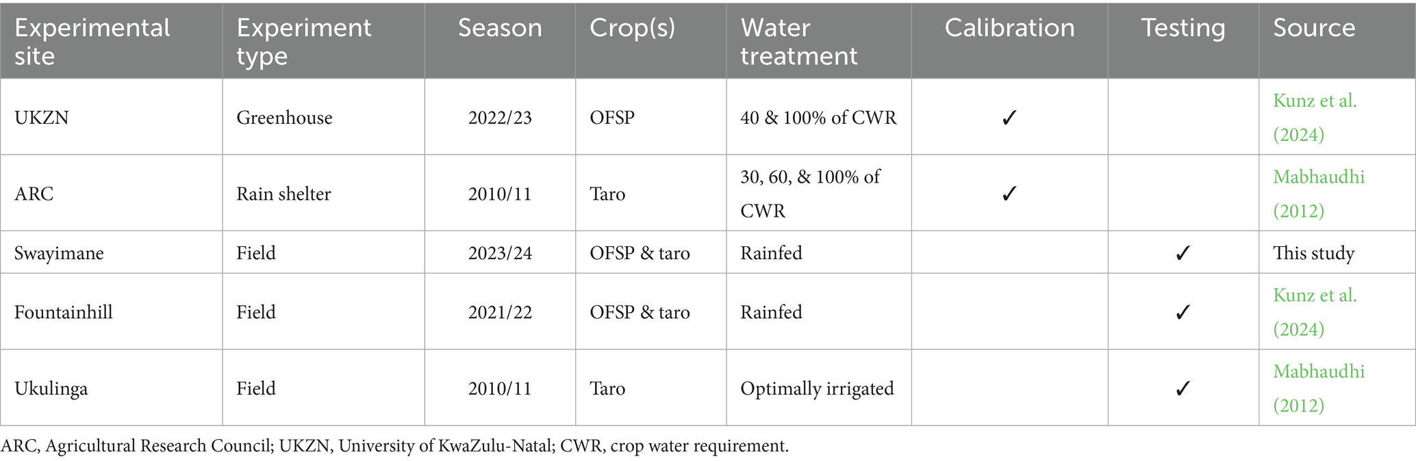
Table 1. Summary of experimental datasets obtained for model calibration and testing of sweet potato and taro in South Africa.

Growth and yield data from the unstressed water treatment (100% of crop water requirement or CWR in mm) were used for recalibration. CWR is the amount of irrigated water required to meet a crop’s maximum evapotranspiration demand (ET_C in mm). The calculation of CWR is based on FAO’s Penman-Monteith equation to calculate ET_O (Allen et al., 1998), which is then adjusted using a crop coefficient (K_C) as follows:

$\begin{array}{ll}CWR=E{T}_C=E{T}_{O}x{K}_C& (4)\end{array}$

For both OFSP and taro experiments, restricted irrigation treatments (40% of CWR for OFSP, and 30 and 60% of CWR for taro) were applied consistently throughout the entire crop development.

For both crops, AquaCrop was validated using data from Swayimane and Fountainhill (Table 1). The latter datasets were sourced from Kunz et al. (2024), who conducted rainfed field experiments over the 2021/22 growing season at Fountainhill (29°27’S; 30°32′E; 851 m a.s.l.), located approximately 32 km north-east of Pietermaritzburg. For this study, data were collected from a smallholder farming community in Swayimane (29°31’S; 30°42′E; 878 m a.s.l.), situated near Wartburg in KwaZulu-Natal, at the end of the 2023/24 season. Another dataset collected by Mabhaudhi (2012) was used to test taro’s recalibration. The irrigated field experiment was undertaken at Ukulinga (29°39’S; 30°24′E; 775 m a.s.l.), UKZN’s research farm located in Pietermaritzburg. Figure 1 shows the location of each experimental site selected for model recalibration and testing.

Figure 1

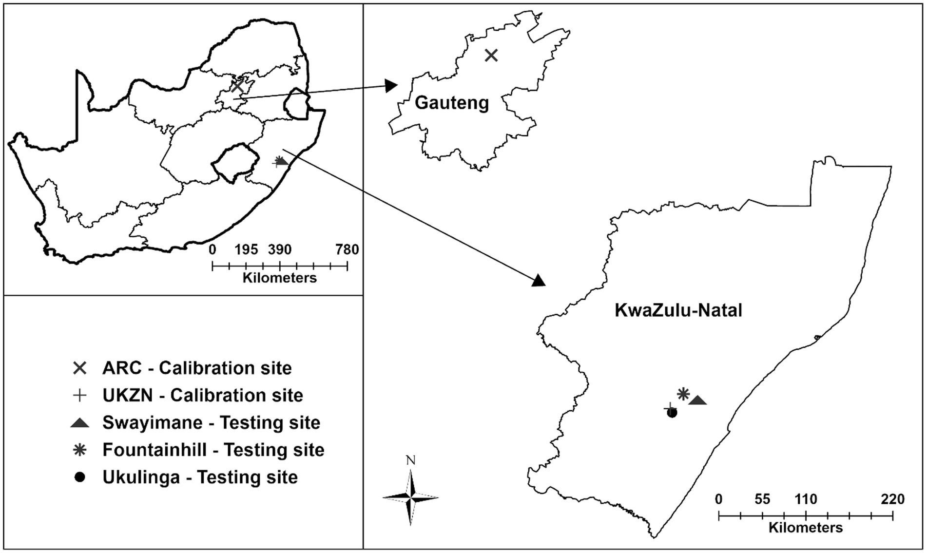
Figure 1. Experimental sites selected for model recalibration and testing of sweet potato and taro in South Africa.

2.3 Model inputs

The original databases for the experimental sites listed in Table 1 were provided by the respective authors. Input data describing soil, climate, and field management were used to develop the corresponding AquaCrop input files for each site, as described below.

2.3.1 Soil data

Data provided in Table 2 were used to develop an input soil (. SOL) file for each experimental site. These include the soil water content at permanent wilting point (PWP), field capacity (FC), and saturation (SAT), as well as total available water (TAW), and saturated hydraulic conductivity (K_SAT). For the Swayimane validation site, soil samples were collected from 0.15, 0.30, and 0.60 m depths using an auger. Soil texture was determined in the soil and water laboratory at UKZN using the hydrometer method (Bouyoucos, 1962). Soil water retention curves were obtained using controlled outflow pressure apparatus and fitted with the Van Genuchten equation (Van Genuchten, 1980), from which soil water content at FC and PWP was estimated at −10 kPa and −1,500 kPa, respectively. K_SAT was measured using the constant-head permeameter method (Klute, 1965).

Table 2

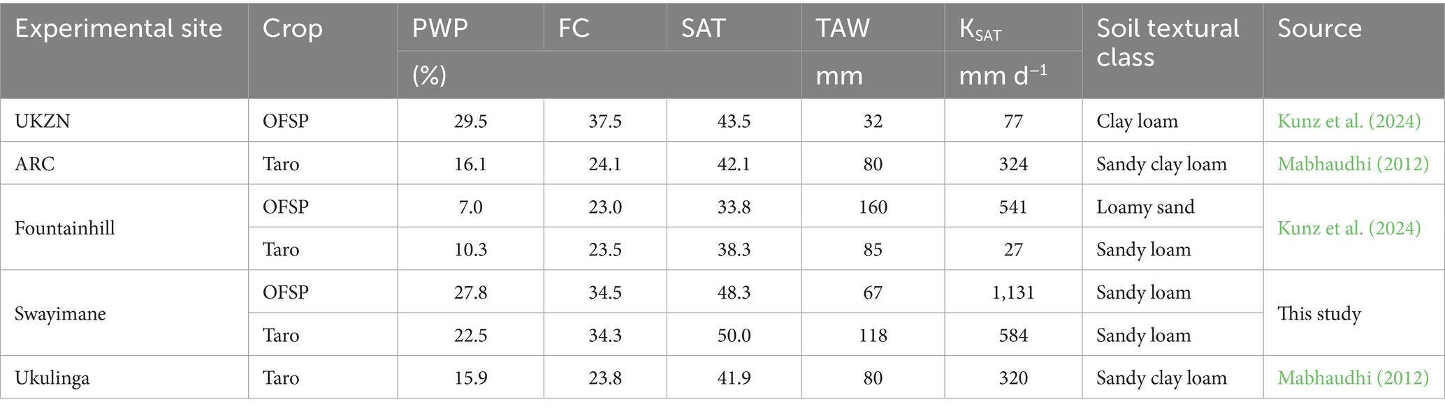
Table 2. Soil data used to develop an AquaCrop soil file for each experimental site.

2.3.2 Climate data

Daily climate files for minimum and maximum air temperature (. TNX) and rainfall (. PLU) were developed using measurements from an automatic weather station (AWS) installed at or near each site by the research team. At the Swayimane, Fountainhill, and Ukulinga validation sites, a Davis Vantage Pro2 AWS was installed. For calibration, climate data were recorded inside the UKZN greenhouse experiment using an AWS of the same type, operated under controlled indoor conditions, while the ARC rain shelter experiment used a similar AWS positioned approximately 100 m from the site. All meteorological sensors were connected to a CR1000 data logger (Campbell Scientific Inc., Logan, Utah, USA). ET_O input files were generated directly in AquaCrop using its internal FAO Penman-Monteith algorithm (Allen et al., 1998), based on daily inputs of solar radiation, wind speed, air temperature, and relative humidity. No external software (e.g., FAO ETo Calculator) was used. For all sites, AquaCrop’s default CO₂ file (MaunaLoa. CO2) was used, which has mean annual values measured at the Mauna Loa Observatory in Hawaii. A summary of the climate data inputs for each site is presented in Table 3.

Table 3

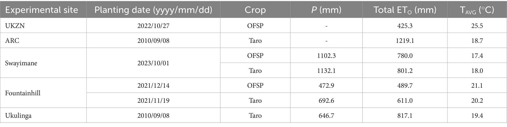
Table 3. Total accumulated precipitation (P), total reference evapotranspiration (ET_O), and average seasonal temperature (T_AVG) for each experimental site.

2.3.3 Management

Irrigation input files (. IRR) were developed for the sites that received irrigation, namely UKZN, ARC, and Ukulinga, which received seasonal totals of 347, 385, and 315 mm, respectively. Irrigation was applied using a drip irrigation system, and the volume of water applied was measured using two inline water meters, which were read after each irrigation event. Groundwater input (. GWT) files were not created as the water table is too deep (> 0.60 m) to influence soil water content in the root zone. Field management (. MAN) files were created for each experimental site to represent actual conditions. OFSP was transplanted using vine cuttings, while taro was planted using cormels. Soil fertility was non-limiting, and no practices were implemented to prevent runoff, such as mulching or soil bunds. Fertilisation, weed control, and pest or disease management were applied according to the protocols of the original experiments used for calibration and validation, which provided all necessary information on these practices.

2.3.4 Initial crop parameters

Attempts to obtain copies of AquaCrop parameter files for OFSP developed locally by Beletse et al. (2013) and Nyathi et al. (2016) were unsuccessful. Furthermore, neither study published a full set of parameterised values. Instead, a sweet potato parameter file developed by Rankine et al. (2015) was obtained from the primary author and utilised in this study. Similarly, the taro parameter file originally developed by Mabhaudhi et al. (2014b) was obtained from the primary author.

2.4 Recalibration procedure

Using guidelines developed by Steduto et al. (2012), model recalibration involved fine-tuning specific parameters initially developed by Rankine et al. (2015) and Mabhaudhi et al. (2014b) to represent local landrace and growing conditions adequately. In AquaCrop, crop parameters are classified as conservative (stable across environments and management practices) or non-conservative (vary with cultivar., location, and management). While conservative parameters are generally stable (FAO, 2023), they were refined in this study to account for the high genetic variability among local landraces. For example, the adjustment of HI_O was done using observations from the non-stressed (i.e., fully irrigated) treatments (cf. Table 1) to ensure that AquaCrop predicts the highest yield under well-watered conditions (FAO, 2023). Other conservative parameters linked to water stress responses (e.g., soil water depletion factors and associated shape factors for canopy expansion, stomatal closure, and senescence) were also fine-tuned. Parameters intrinsic to crop species, such as the cut-off temperature for development, were retained to avoid compromising accuracy. For parameters that were not measured (e.g., basal crop coefficient), representative values were sourced from literature (e.g., Pereira et al., 2021).

Non-conservative parameters should be fine-tuned to improve model performance for different cultivars, landraces, and environmental conditions (FAO, 2023). Therefore, the canopy growth coefficient (CGC) and canopy decline coefficient (CDC) parameters were recalibrated to better capture CC development. For taro, CC was estimated by Mabhaudhi et al. (2014b) using Diffuse Non-Interceptance measurements obtained with an LAI-2200 Plant Canopy Analyzer (LI-COR, 2009). For OFSP, Kunz et al. (2024) derived CC indirectly by converting measured leaf area index values using the Beer–Lambert law (Swinehart, 1962). At the Swayimane validation site, the same approach was employed to convert measured leaf area index values to CC.

The time (in calendar days) to reach each phenological growth stage (i.e., emergence, maximum rooting depth, canopy senescence, maturity, and yield formation) was also adjusted to improve simulation accuracy. However, this was affected by the lack of measurements during the initial growth period at some sites. Canopy senescence begins when the chlorophyll content of upper leaves declines or when 10% of lower leaves begin to yellow under non-stressed conditions (Mabhaudhi, 2012). The physiological maturity date occurs when root/tuber growth stabilises. Despite flowering being linked to the photoperiod for root and tuber crops (RTCs), it does not occur often, especially for sweet potato (Rankine et al., 2015) and taro (Mabhaudhi, 2012). Hence, the start and duration of flowering were set to zero.

All adjustments were made iteratively through a trial-and-error process until model simulations aligned closely with observed data. AquaCrop was run in calendar day mode, which is the standard approach in parameterisation and calibration studies. AquaCrop v7.1 (FAO, 2023) was used, with the simulation period linked to the growing cycle, i.e., day one after sowing up to physiological maturity. For OFSP and taro, planting dates were set at 27 October 2022 and 8 September 2010, respectively (cf. Table 3). Planting densities were set to 55,556 and 20,000 plants per ha⁻¹ for OFSP and taro, respectively. These settings were applied to mimic experimental conditions.

2.5 Validation procedure

AquaCrop was validated for both crops using data from Fountainhill and Swayimane, with an additional site (Ukulinga) used for taro (cf. Table 1). These locations span a range of agro-climatic conditions, enabling an evaluation of model robustness across different environments. AquaCrop was run in thermal time (i.e., GDD mode), which standardises phenological development against heat accumulation rather than calendar days. No recalibration was performed during validation, ensuring that the model’s predictive capability was reflected under independent conditions. Including multiple sites served to assess the model’s transferability and identify potential limitations in performance under diverse locations.

2.6 Model evaluation statistics

Model performance was quantified by comparing simulated and observed CC development (in %), biomass production and harvestable yield (both in t ha⁻¹), and HI (in %). As suggested by Chibarabada et al. (2020), the following statistical indicators were used to evaluate model performance since each statistic offers specific advantages and drawbacks: coefficient of determination (R²), root mean square error (RMSE), normalised RMSE (NRMSE), Nash-Sutcliffe model efficiency (NSE), and Willmott’s index of agreement (d-index), including the percentage error (i.e., deviation).

3 Results and discussion

3.1 Model recalibration

Recalibrated values for selected crop parameters are presented in Table 4 and Table 5 for OFSP and taro, respectively. The inclusion of additional parameters reflects a commitment to transparency, relative to 23 and 26 values published by Rankine et al. (2015) and Mabhaudhi et al. (2014b), respectively.

Table 4

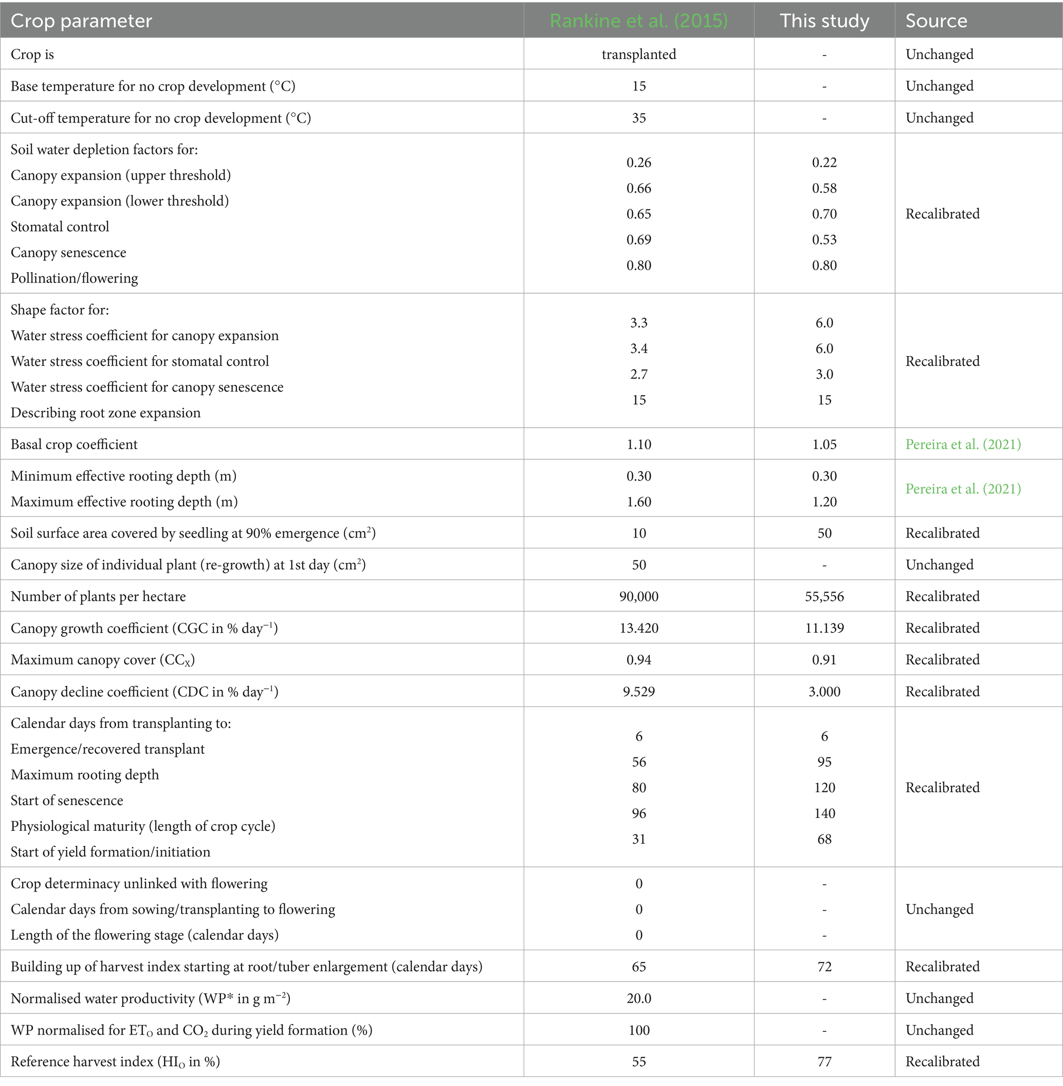
Table 4. Comparison of important parameters derived by Rankine et al. (2015) for sweet potato, to those fine-tuned in this study for OFSP.

Table 5

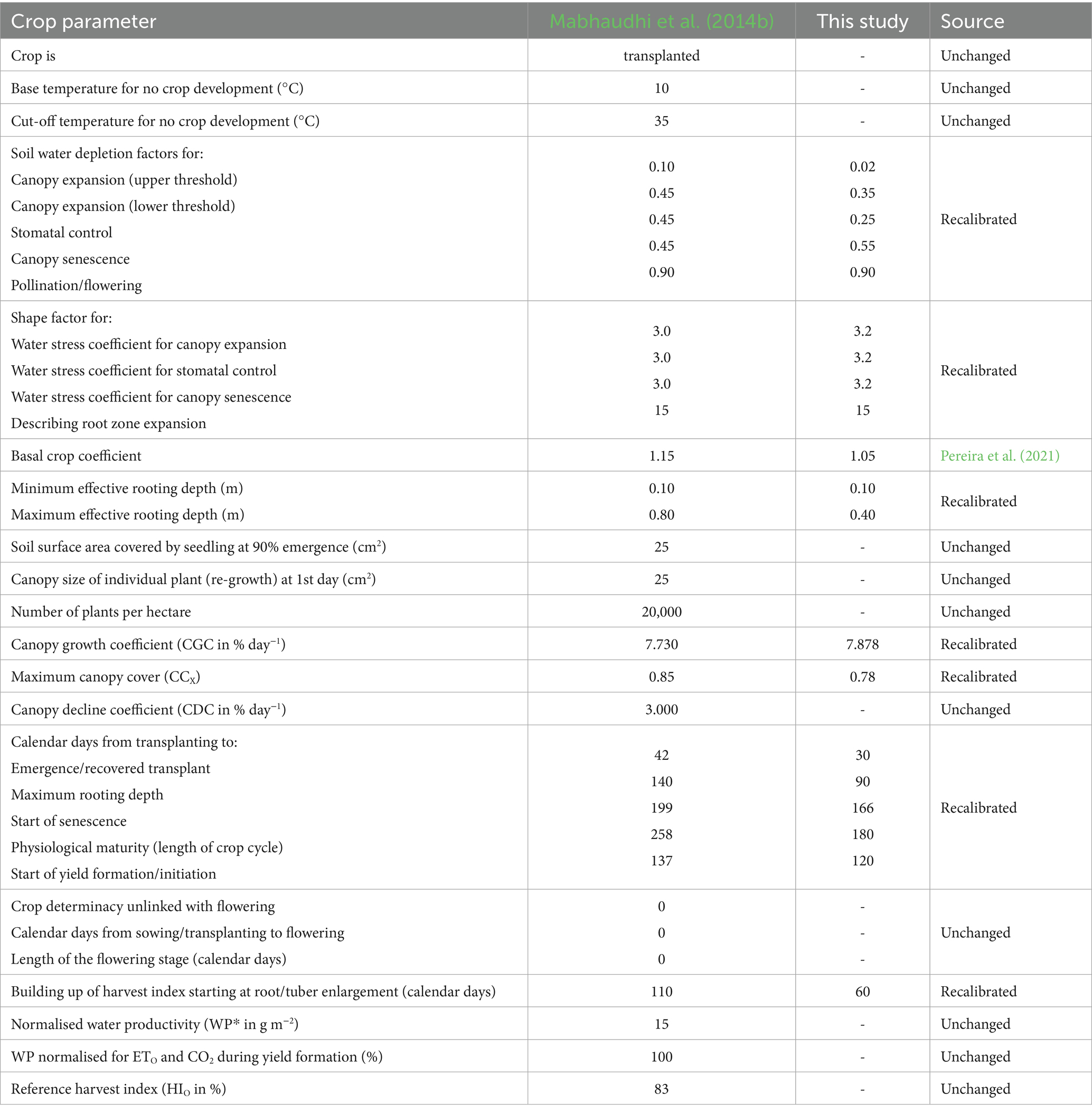
Table 5. Comparison of taro parameters derived by Mabhaudhi et al. (2014b) to those fine-tuned in this study.

3.1.1 Canopy cover development

For OFSP, AquaCrop simulations showed a good match (0.925 ≤ R² ≤ 0.954; 6.186 ≤ MAE ≤ 9.485%; 7.537 ≤ RMSE ≤ 11.434%; 9.372 ≤ NRMSE ≤ 14.098%; 0.765 ≤ NSE ≤ 0.880; 0.940 ≤ d-index ≤ 0.975) between observed and simulated CC values for both the unstressed (100% of CWR) and stressed (40% of CWR) treatments (Figure 2). The R² and RMSE statistics showed better model performance relative to those obtained by Nyathi et al. (2016), which were 0.77 and 12.10%, respectively. However, AquaCrop mostly over- and under-estimated CC development for the unstressed and stressed treatments, respectively, which aligns with findings by Rankine et al. (2015). Improvements in CC simulation accuracy are not only a technical calibration success but also enhance the model’s operational value for real-world applications such as predicting growth trajectories under climate stress. Accurate CC simulation allows for better estimation of light interception and evapotranspiration patterns, which are critical for yield forecasting and water resource planning, especially in water-scarce environments.

Figure 2

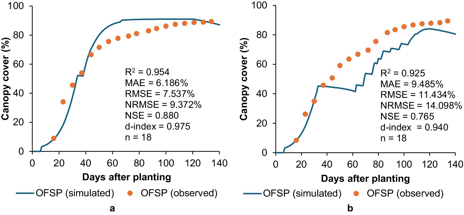
Figure 2. Simulated versus observed canopy cover development for OFSP grown under (a) unstressed and (b) stressed conditions in a greenhouse at UKZN during the 2022/23 season.

The CGC parameter in AquaCrop determines the rate of initial CC development, which generally follows a concave shape for most crops (FAO, 2023). However, OFSP’s CC development initially followed a convex-shaped curve, thus highlighting very rapid crop development during the early growth stages (Figure 2). To mimic this behaviour, the parameter representing the soil surface area covered by an individual seedling was adjusted to the highest permissible value of 50 cm² for a transplanted crop (cf. Table 4). OFSP rapidly establishes ground cover, which is consistent with the vigorous vegetative growth trait of RTCs (Mabhaudhi, 2012; Masango, 2015). This rapid establishment is facilitated by OFSP’s method of propagation, as the crop is transplanted using vine cuttings rather than being grown from seed, which facilitates immediate vegetative growth from established nodes. Rapid canopy closure reduces the soil evaporation window, improves early-season soil moisture conservation, and provides a competitive advantage against weed establishment. Simulating this accurately is essential for realistic water productivity estimates and designing planting strategies that optimise early-season resource capture.

For taro, model evaluation showed a moderate to good agreement (0.519 ≤ R² ≤ 0.632; 6.005 ≤ MAE ≤ 9.408%; 7.193 ≤ RMSE ≤ 9.615%; 25.675 ≤ NRMSE ≤ 34.840%; 0.044 ≤ NSE ≤ 0.485; 0.757 ≤ d-index ≤ 0.773) between simulated and observed CC values for the unstressed (100% of CWR) and moderately stressed (60% of CWR) treatments (Figure 3). RMSE and NRMSE values were lower relative to those generated using the original crop file by Mabhaudhi et al. (2014b), which ranged from 10.123–16.817% and 46.614–54.862%, respectively. Thus, the recalibrated crop parameters are better than the original values. This improvement has practical significance as better CC prediction for taro in moderately stressed environments suggests that the model can be used as a decision-support tool to reliably inform farmers and policymakers about potential yield reductions under water-limited scenarios, enabling proactive adaptation measures such as irrigation scheduling or mulching.

Figure 3

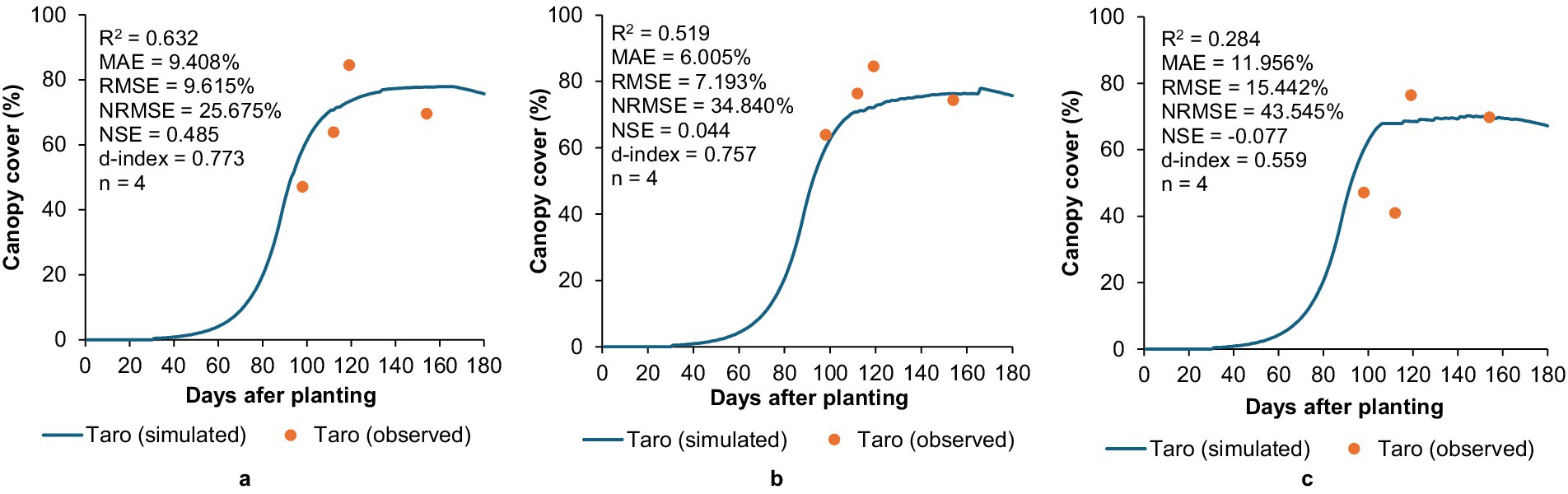
Figure 3. Simulated versus observed canopy cover development for taro under (a) unstressed, (b) moderately stressed, and (c) stressed growing conditions under the rain shelter at Roodeplaat during the 2010/11 season.

Measured CC development was highest at 119 days after planting (DAP) across all treatments. This indicates crop senescence occurred between 119 to 154 DAP, which the model did not simulate well. This discrepancy suggests that the CDC senescence parameter may require further calibration. Additionally, it may indicate that the model does not fully account for the physiological ageing of taro or possible stress factors (e.g., nutrient depletion or disease onset) that could have triggered earlier or more rapid senescence as was observed. Identifying and addressing these gaps is essential for improving predictive reliability under variable nutrient and pest pressures, which are conditions that are common in smallholder systems.

AquaCrop showed limited accuracy in simulating taro’s CC development under water-stressed conditions (Figure 3). The negative NSE (−0.077) suggests that predictions had a higher error variance relative to variability in observations. This highlights AquaCrop’s inability to adequately simulate taro’s CC development under water-stressed conditions, which was also noted by Mabhaudhi et al. (2014b). This limitation may suggest the need for further refinement of taro’s water stress response parameters. From a broader perspective, this indicates that AquaCrop’s current structure may not fully capture the physiological and morphological adaptations of taro under severe drought. For decision-makers relying on these simulations, particularly in climate-vulnerable regions, such underperformance under water stress could underestimate the urgency of adaptation interventions needed.

For the stressed treatment, MAE (11.956%) was lower than RMSE (15.442%), which is expected as the latter statistic is more sensitive to outliers. Observed CC development increased sharply from 41% at 112 DAP to 76% at 119 DAP, which raises concerns about data validity. This highlights the importance of scrutinising data from secondary sources for potential errors before being used for model calibration. This also reflects a common challenge in modelling under-researched crops as the scarcity of high-quality field data can limit calibration quality and mask true crop-environment interactions, which in turn reduces confidence in long-term projections.

The low NSE values for the moderately stressed and stressed treatments also highlight that this statistic is sensitive to a low number of observations (McCuen et al., 2006). In contrast to the OFSP dataset (Figure 2), only four CC measurements were made. The lack of observations during the early growth stages hindered the ability to accurately recalibrate initial CC development, thus limiting the robustness of model validation. This issue highlights the importance of improving the quality of in situ datasets by ensuring that measurements span the entire growing season to support effective model calibration. From an applied research standpoint, this finding reinforces the need for systematic phenotyping campaigns for NUS across agro-ecologies. Such efforts would enable stronger model parameterisation and reduce uncertainty in growth predictions, ultimately improving advisory services for farmers.

The simulated CC development curves for OFSP (Figure 2) and taro (Figure 3) did not decline towards the end of the season. This can be attributed to their stay-green trait (Adugna and Tirfessa, 2014; Wirojsirasak et al., 2024), which enables both crops to retain leaf chlorophyll for prolonged periods during their latter growth stages. This stay-green trait makes it difficult to determine the start of senescence. For both crops, the model’s CDC parameter was therefore set to the lowest value of 3% to prevent the decline in CC development as the crop approaches physiological maturity. Accurately representing stay-green behaviour is particularly relevant for climate adaptation modelling, as it is linked to drought resilience and sustained photosynthesis under late-season stress. Failure to simulate it correctly could lead to underestimation of yield stability in marginal environments, which is crucial for positioning NUS as climate-resilient alternatives to conventional staples.

3.1.2 Above-ground biomass production

Based on high R² (0.985–0.989) and d-index (0.817–0.871) values, AquaCrop adequately captured above-ground biomass production for OFSP under (a) unstressed and (b) stressed treatments, despite the consistent over-simulation (Figure 4). The other metrics (MAE, NRMSE, and NSE) suggest the model was less successful in simulating biomass production under stressed conditions, compared to the unstressed treatment. The decline in NSE from 0.521 to 0.138 highlights the model’s inability to adequately simulate crop physiology under water deficit conditions. This again suggests the need for improving the model’s response to water-limiting conditions. This limitation is critical as biomass accumulation directly influences yield and water productivity estimates. If stressed-condition biomass is overestimated, water-saving interventions may not be implemented, potentially leading to misallocation of scarce irrigation resources in practice.

Figure 4

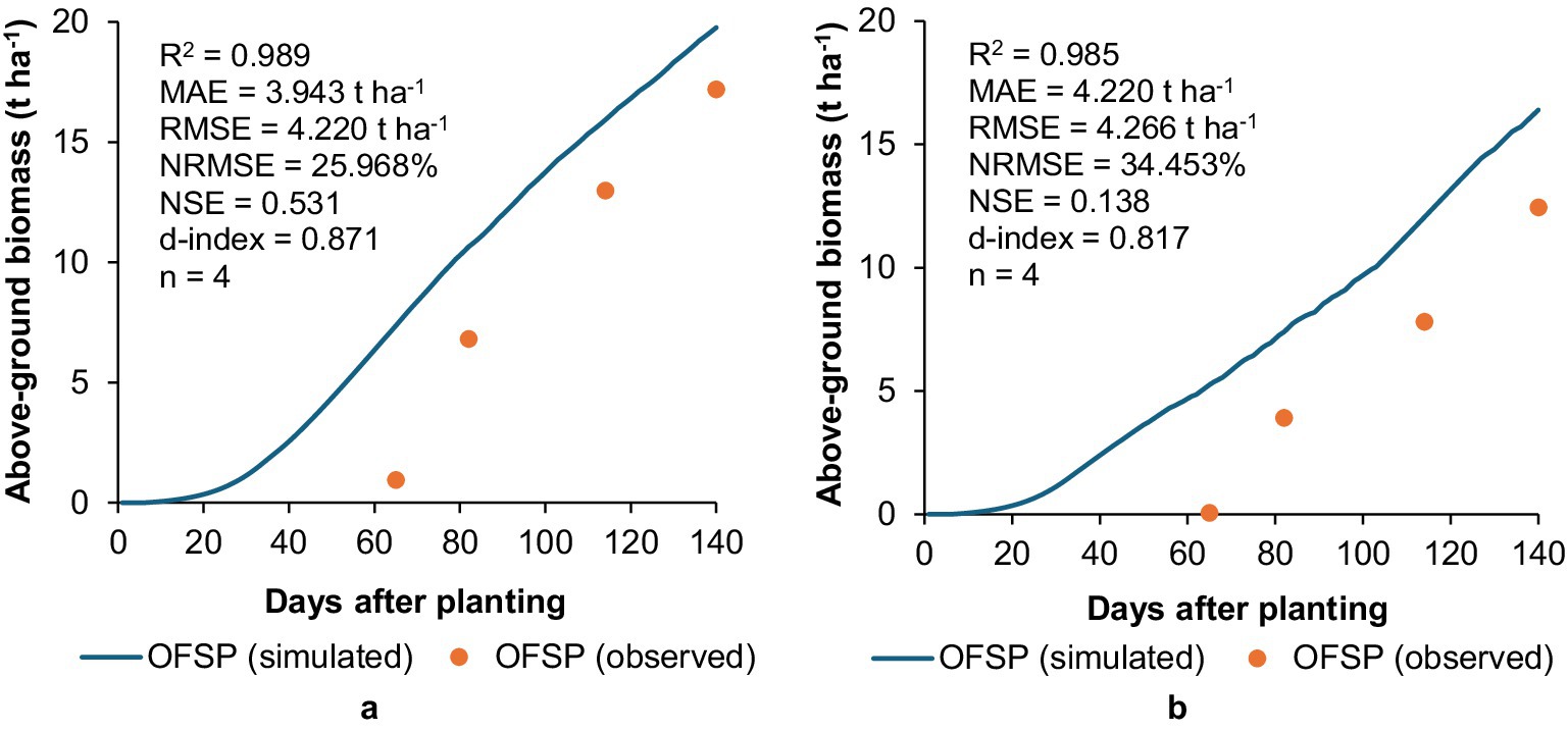
Figure 4. Simulated versus observed above-ground biomass accumulation for OFSP grown under (a) unstressed and (b) stressed conditions in a greenhouse at UKZN during the 2022/23 season.

From Figure 5, all model evaluation statistics highlight AquaCrop’s ability to accurately simulate above-ground biomass production for taro, despite the slight decline in model performance for the stressed treatment. These results suggest that AquaCrop reliably captures biomass accumulation in taro across varying water regimes, although further refinement may be needed to enhance its sensitivity to stress conditions. For agricultural planning, this means AquaCrop could be a viable decision-support tool for taro yield estimation under moderate to optimal water availability but would require caution or further calibration before being used for drought-response planning in severely water-stressed areas.

Figure 5

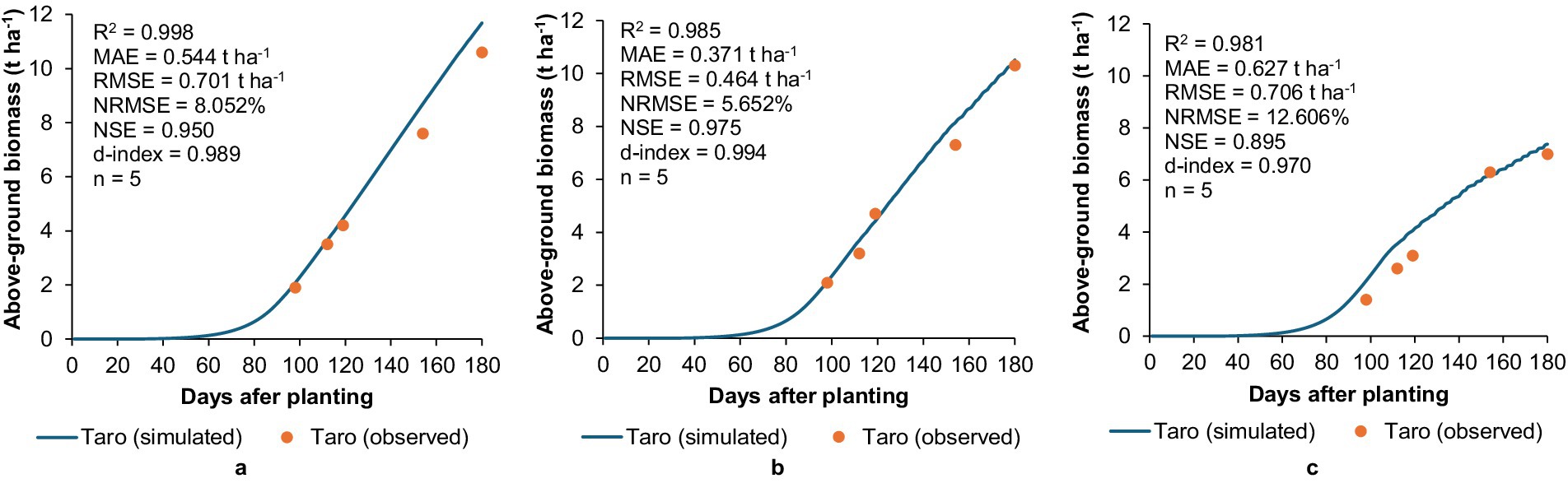
Figure 5. Simulated versus observed above-ground biomass production for taro under (a) unstressed, (b) moderately stressed, and (c) stressed conditions at Roodeplaat during the 2010/11 season.

3.1.3 Final biomass and yield at harvest

Model performance for final above-ground biomass, yield, and HI using the recalibrated crop parameters is summarised in Table 6. AquaCrop simulated all three variables with high accuracy, particularly for OFSP. Absolute deviations are within 6%, which is considered negligible by Dua et al. (2014). The model simulated high HI values for both crops, which ranged from 76 to 88% under all treatments. This was influenced by the high reference HI parameter for both crops.

Table 6

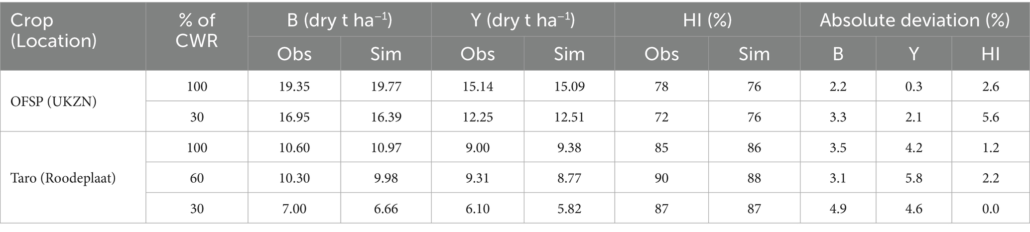
Table 6. Observed (obs) and simulated (sim) above-ground biomass (B), yield (Y), and harvest index (HI) for OFSP and taro after model recalibration.

Prior to recalibration (i.e., using parameters derived by Rankine et al., 2015), above-ground biomass simulations were reasonable with absolute deviations of 3.9–15.4%. However, the model under-estimated yield due to a low HI (~50%), with absolute deviations ranging from 30.3–45.5%. These simulations were conducted in a previous study by Rankine et al. (2015). This suggests that HI varies substantially across different sweet potato cultivars and landraces. Hence, deriving a reference value that is universal for all sweet potato genotypes will prove difficult. Similarly, AquaCrop grossly over-estimated taro’s biomass and yield, especially for the fully irrigated treatment, as indicated by Mabhaudhi et al. (2014b). These differences highlight the need to recalibrate the crop parameters, i.e., the main aim of this study. The implication is that default parameter sets, often used where local data is lacking, may lead to highly misleading outputs for NUS, emphasising the necessity for site and genotype specific calibration before operational deployment.

The marked improvement in absolute deviations for taro’s biomass and yield (Table 6) is due to the adjustments made in crop parameters to reflect better the crop’s growth and response to water stress. Reducing the model’s soil water depletion factors for canopy expansion and stomatal control, enhanced its ability to simulate water stress effects on taro growth (cf. Table 5). Additionally, lowering maximum CC (from 0.85 to 0.78) and maximum rooting depth (from 0.80 to 0.40 m) prevented the model from over-estimating taro’s biomass and yield for each treatment. This adjustment aligns with findings that taro is a shallow-rooted crop, typically developing roots within the top 30–45 cm of soil (Onwueme, 1999), thereby limiting its access to deeper soil moisture under stress conditions. By accurately constraining rooting depth, the model can now more realistically assess taro’s vulnerability to in-season dry spells, making it more suitable for climate risk modelling in shallow-soil agro-ecological zones.

Phenological calibration posed challenges due to limited early growth observations and taro’s stay-green trait, which prevents canopy decline from signalling maturity. AquaCrop does not simulate this behaviour, assuming instead a direct link between senescence and tuber maturity. For RTCs such as OFSP and taro, physiological maturity can be more reliably indicated by the stabilisation of tuber mass than by the onset of leaf senescence, which has been demonstrated in various RTC studies. For example, Kunz et al. (2024) observed that for taro, tuber yield stabilised between 180 and 191 DAP, but the crop was harvested at 206 DAP. Similarly, observations at Fountainhill, one of the sites used for model validation, showed that OFSP tuber yield stabilised around 105 DAP, yet harvesting occurred at 118 DAP. To address this issue, phenological growth stages for taro, such as the time to reach maximum rooting depth, senescence, and yield formation, were shortened to reflect actual crop growth dynamics, which resulted in improved yield predictions. In practical terms, using tuber mass stabilisation as a maturity indicator could improve harvest-timing recommendations, reduce post-maturity losses and improve resource-use efficiency, which is particularly important for resource-constrained farmers seeking to maximise yield under climate-stress.

The recalibration of AquaCrop for OFSP and taro was improved by adjusting 21 and 19 parameters, respectively (cf. Section 3.1). This is comparable to Mabhaudhi et al. (2014a, 2014b), where 21 parameters were adjusted to parameterise the model for bambara groundnut and taro. With these refinements, AquaCrop reliably simulated biomass and yield for both crops under unstressed and stressed conditions. The latter outcome is different to other studies (e.g., Patel et al., 2008; Heng et al., 2009; Hsiao et al., 2009), which highlighted AquaCrop’s inability to adequately simulate maize and potato yield under water-stressed conditions. Rankine et al. (2015) highlighted the difficulty of calibrating RTCs relative to major staples; the present study demonstrates that targeted recalibration can overcome these challenges, producing predictive performance on par with or better than that for conventional crops. This strengthens the case for mainstreaming NUS in crop modelling portfolios and integrating them into climate adaptation and food security policies.

To date, AquaCrop v7.1 has been parameterised for 17 herbaceous crops using data collected from 1978 to 2019 across 28 locations (Raes et al., 2023). For example, Raes et al. (2023) stated that potato has the least reliable AquaCrop parameterisation relative to other crops, which is based on experimental data from 1995 for a single site. This raises concerns when using default crop parameters to simulate the growth and yield of recent cultivars. Genetic modifications have enhanced disease resistance, nutritional value, and yield of crops over the past decades. For example, modern plant breeding tools and molecular manipulation techniques, such as TALENS, CRISPR-Cas9, RNAi, and cisgenesis, have been used to improve potato yield and nutritional content (Ahmad et al., 2022). Since genetic improvements are continually phasing out old cultivars, regular recalibration of crop models is necessary to reflect these advancements.

3.2 Model validation

Crop parameters should produce reliable results across a wide range of acro-ecological zones. Therefore, AquaCrop’s ability to simulate CC development, above-ground biomass, yield, and HI was tested against secondary datasets obtained from experiments conducted at Fountainhill (rainfed), Swayimane (rainfed), and Ukulinga (optimally irrigated) (cf. Table 1). For model validation, AquaCrop was run in GDD mode to account for climatic variations between the calibration locations and validation sites.

3.2.1 Canopy cover development

AquaCrop performed poorly in simulating CC development for OFSP at Fountainhill under rainfed conditions compared to Swayimane (Figure 6). Relatively high R² values can be misleading as models may perform poorly by grossly under- or over-estimating measured data (Krause et al., 2005), which highlights the importance of considering other statistical indicators to evaluate models. If the simulation of CC development at Fountainhill was delayed, resulting in the curve shifting to the right (Figure 6a), the correlation would be substantially improved. This discrepancy may be attributed to site-specific microclimatic conditions during the study period, which may have constrained AquaCrop’s parameterisation of early-stage canopy development at this site. For decision-making, this highlights the importance of site-specific model calibration, as a single recalibration may not always account for factors across multiple sites during validation. Accurate simulation of early canopy development is critical, as errors at this stage can cascade into biomass and yield overestimations. Similar challenges have also been reported by Rankine et al. (2015), where AquaCrop simulations for sweet potato did not agree well with measured values.

Figure 6

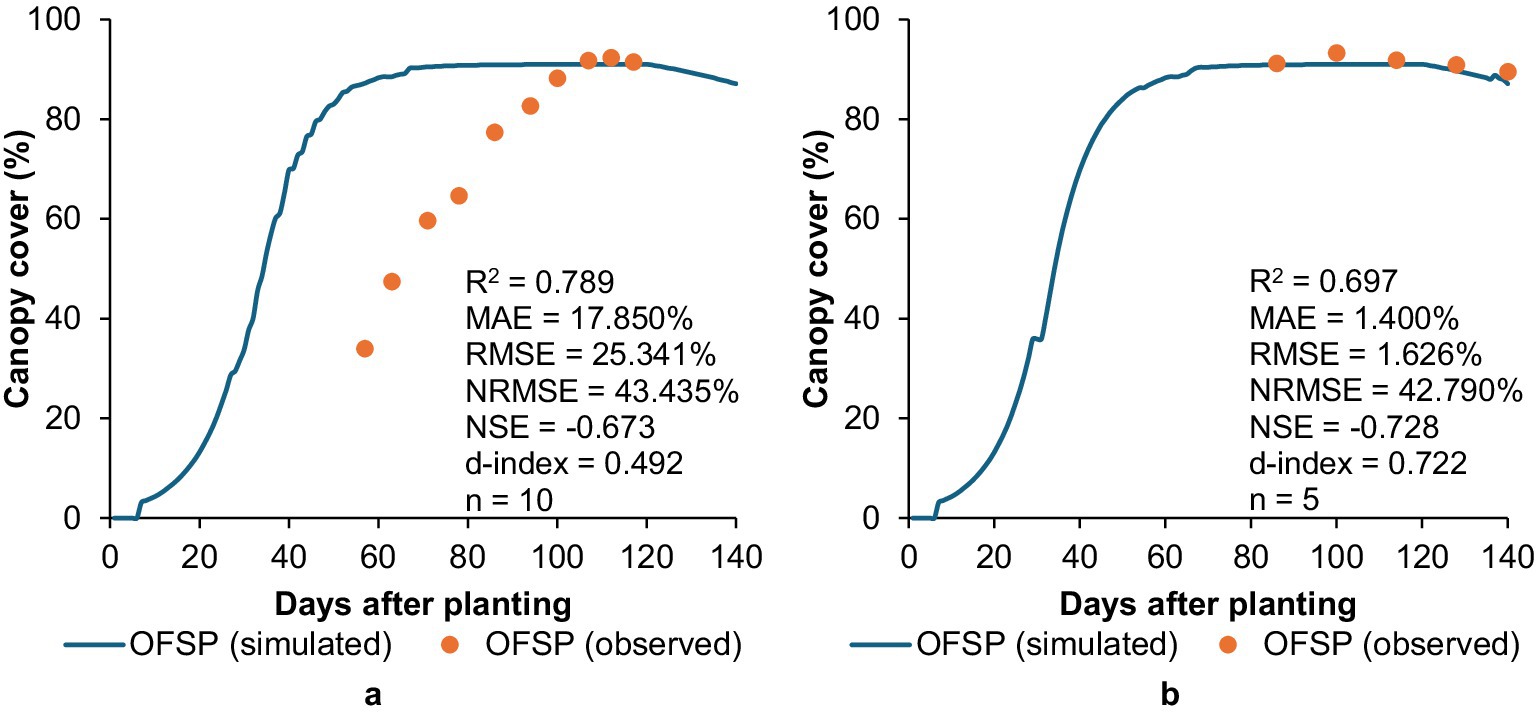
Figure 6. Validation results showing the comparison between simulated and observed canopy cover development for OFSP grown at (a) Fountainhill and (b) Swayimane under rainfed conditions.

The model performed well at Swayimane by accurately simulating CC development for OFSP, achieving MAE, RMSE, and d-index values of 1.400, 1.626%, and 0.722, respectively. However, the NRMSE (42.790%) and NSE (−0.728) statistics for Swayimane indicate a poor simulation, which is likely influenced by the low number of observations (n = 5). Early canopy data were missing due to logistical constraints, as the trials were embedded within a larger multi-crop experiment with limited monitoring resources. This gap reduces confidence in early-stage validation and illustrates a common limitation in underutilised crop research, where resource constraints often restrict high-resolution data collection. Future studies should prioritise season-long monitoring to support more robust model testing.

AquaCrop over-estimated CC development for taro at Fountainhill (Figure 7a) and Ukulinga (Figure 7c), with overall poor model performance at both sites (0.332 ≤ R² ≤ 0.564; 7.257 ≤ MAE ≤ 16.753%; 8.381 ≤ RMSE ≤ 19.745%; 63.695 ≤ NRMSE ≤ 64.466%; −3.450 ≤ NSE ≤ −2.046; 0.540 ≤ d-index ≤ 0.566). While this over-estimation may stem from inaccuracies in parameters governing early canopy development, including the time to transplant recovery, initial CC, the CGC, and time to reach maximum CC, climatic factors play a more substantial role. Rainfall at these two sites (692.6 mm at Fountainhill and 646.7 mm at Ukulinga) was considerably lower relative to 1132.1 mm at Swayimane (cf. Table 3). AquaCrop generally performs better when simulating non-stressed conditions (FAO, 2023). This was corroborated at Swayimane (Figure 7b), where the higher rainfall likely contributed to the model’s excellent simulation of CC development (R² = 0.999; MAE = 1.240%; RMSE = 1.741%; NRMSE = 3.922%; NSE = 0.989; d-index = 0.998). This strong agreement indicates the model is well-suited to simulating conditions with no water stress, i.e., AquaCrop’s predictive accuracy declines when modelling water-limited environments (Steduto et al., 2009; FAO, 2023). This confirms that water stress remains a key weakness in AquaCrop’s performance for NUS, meaning its outputs should be interpreted with caution for drought-prone areas unless stress-response parameters are further improved.

Figure 7

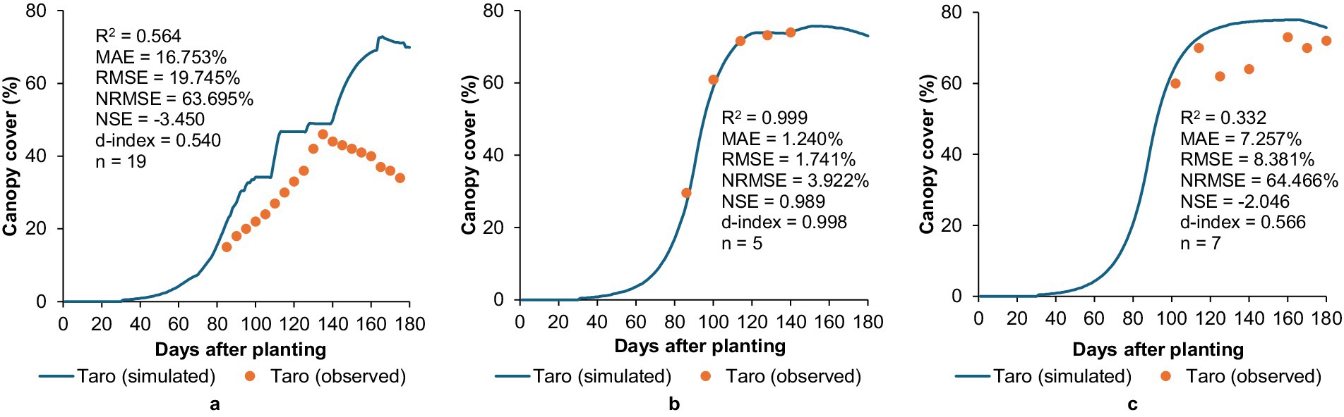
Figure 7. Validation results showing the comparison between simulated and observed canopy cover development for taro at (a) fountainhill, (b) swayimane, and (c) Ukulinga.

3.2.2 Above-ground biomass production

AquaCrop adequately captured the trend in above-ground biomass production for OFSP grown at (a) Fountainhill and (b) Swayimane (Figure 8), as shown by the high R² values (0.959–0.999). Despite the good NSE (0.632) and d-index (0.834) statistics, high MAE (4.043 t ha⁻¹), RMSE (4.475 t ha⁻¹), and NRMSE (22.671%) values highlighted the model’s inability to predict biomass production for OFSP grown at Fountainhill accurately. This was expected since biomass prediction is directly related to the model’s ability to simulate CC development (cf. Figure 6a). The lower model performance at Fountainhill can also be attributed to excessive weed growth after planting, which delayed the collection of biomass data until 57 DAP (Kunz et al., 2024). This suggests that early crop development was suboptimal in the field and underrepresented in the observed dataset, which limited the accuracy of the model evaluation during the initial growth stages. In operational terms, this shows that unaccounted field factors, like weed pressure, can significantly reduce the reliability of model outputs and must be documented alongside calibration datasets to avoid misinterpretation of deviations.

Figure 8

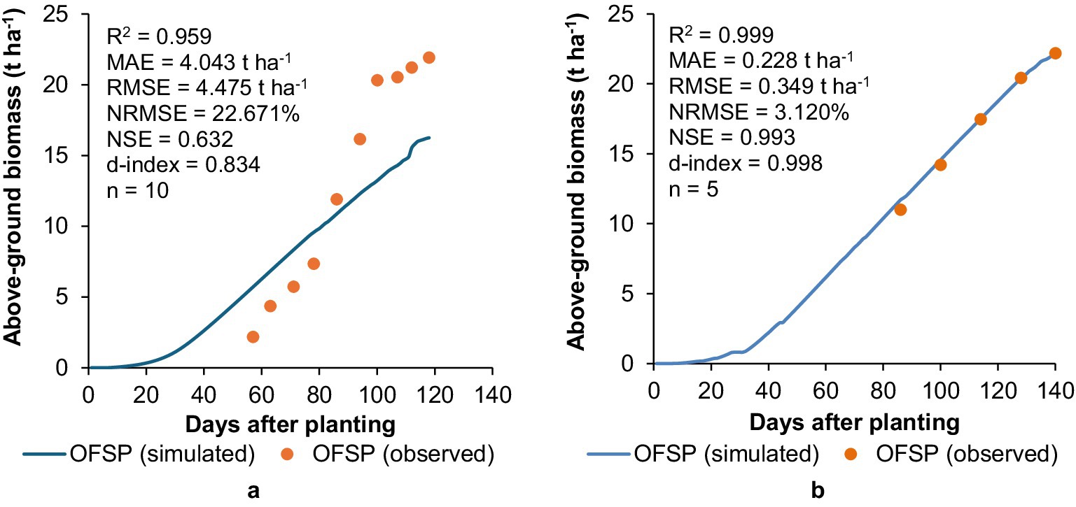
Figure 8. Validation results showing a comparison between simulated and observed above-ground biomass accumulation for OFSP at (a) fountainhill and (b) swayimane.

This is further supported by AquaCrop’s accurate simulation of CC development at Swayimane (cf. Figure 6b), which resulted in an excellent above-ground biomass simulation (R = 0.999; MAE = 0.228 t ha⁻¹, RMSE = 0.349 t ha⁻¹, NRMSE = 3.120%, NSE = 0.993; d-index = 0.998) at this site. This strong performance is again attributed to the high rainfall at Swayimane, which resulted in non-stressed growing conditions. This suggests that for reliable biomass predictions, AquaCrop is currently best suited to regions where supplementary irrigation or consistently high rainfall minimises water stress variability. This finding is consistent with previous research on underutilised crops, where AquaCrop performs reliably under favourable water conditions but with limited accuracy under water stress (Mabhaudhi, 2012; Mabhaudhi et al., 2014a; Rankine et al., 2015).

AquaCrop accurately simulated the biomass accumulation for taro at Swayimane (Figure 9), with excellent model evaluation statistics (R² = 1.000; MAE = 0.084 t ha⁻¹; RMSE = 0.089 t ha⁻¹; NRMSE = 1.240%; NSE = 0.999; d-index = 1.000), further highlighting the model’s suitability for simulating unstressed conditions. Model performance at Ukulinga was satisfactory as indicated by adequate statistics (R² = 0.977; NSE = 0.801; d-index = 0.929). Despite taro grown at Ukulinga receiving 647 mm of rainfall and 315 mm of supplemental irrigation to relieve any water stress (cf. Table 3), AquaCrop under-estimated taro’s above-ground biomass towards the latter stages of the growing season, as indicated by relatively high MAE (1.996 t ha⁻¹), RMSE (2.786 t ha⁻¹), and NRMSE (15.251%) values.

Figure 9

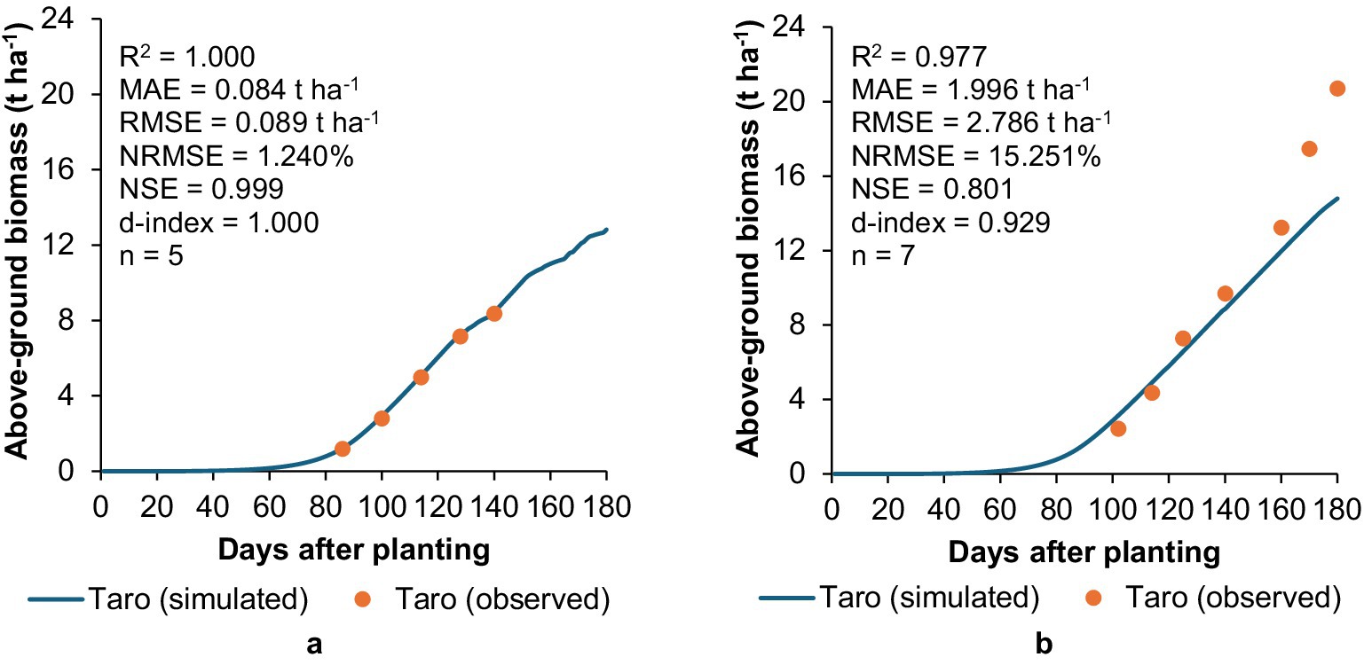
Figure 9. Validation results showing a comparison between simulated and observed above-ground biomass accumulation for taro at (a) swayimane and (b) ukulinga.

3.2.3 Final biomass and yield at harvest

AquaCrop predicted final yield at Fountainhill and Swayimane adequately with absolute deviations between observations and simulations ranging from 6.8–11.9% for OFSP and 0.3–5.3% for taro (Table 7). The model exhibited acceptable deviations for taro’s final above-ground biomass at Fountainhill (1.2%) and Swayimane (7.9%). These results suggest that only minimal model calibration may be required when applying AquaCrop to other OFSP and taro landraces growing in similar agro-ecological zones. For practitioners, this means once a robust calibration is done for a representative landrace in a given area, it may be applied to other nearby areas with only minor adjustments, reducing the time and cost barriers to using modelling for production planning.

Table 7

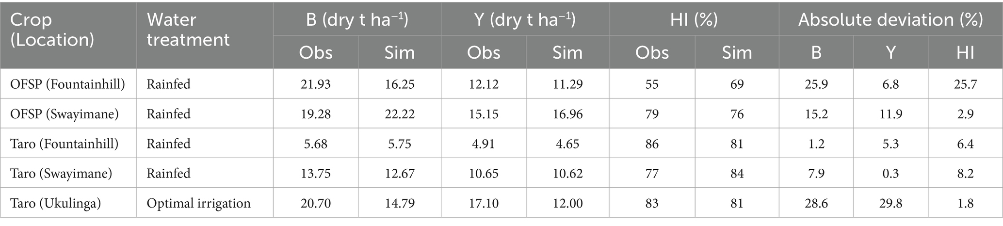
Table 7. Observed (obs) and simulated (sim) above-ground biomass (B), yield (Y) and harvest index (HI) for OFSP and taro obtained during model testing.

However, larger absolute deviations (15.2–28.6%) in final above-ground biomass were identified for OFSP at Fountainhill and Swayimane, and for taro at Ukulinga. This indicates the model may inadequately simulate final biomass across different locations. AquaCrop predicted the HI of OFSP at Swayimane and taro at Fountainhill, Swayimane, and Ukulinga with high accuracy (Table 7). However, the model failed to simulate the HI for OFSP at Fountainhill accurately. Given that HI directly affects yield estimation, inaccuracies in HI modelling under certain site conditions may undermine AquaCrop’s utility for harvest predictions unless these specific weaknesses are addressed in future recalibrations.

Differences in model performance for various OFSP and taro landraces at different locations may be influenced by genotypic variability. Landraces typically exhibit high genetic variation and are adapted to specific environments. Different landraces, therefore, have varying biomass accumulation rates, growth patterns, and yield potentials. The calibration for a specific landrace may therefore not be suitable for others, especially across diverse agro-ecological zones. This highlights the importance of calibrating AquaCrop using pooled data representing multiple landraces grown at different locations to improve its predictive performance, thus ensuring robust validation. This approach would also support scaling AquaCrop beyond research into policy and extension work, allowing it to inform crop diversification strategies at provincial or national levels.

From the literature, HI values ranged from 22 to 90% for OFSP (Bouwkamp and MHM, 1988; Bhagsari and Doyle, 1990; Beletse et al., 2013; Rankine et al., 2015) and 50 to 83% for taro (Mabhaudhi et al., 2014b). While part of this variability can be explained by the genetic diversity of NUS, which consist of multiple landraces with distinct physiological traits, climatic and management factors are equally critical drivers of HI variability. For instance, higher rainfall and favourable conditions at Swayimane promoted more effective assimilate partitioning to storage roots, whereas at Fountainhill, weed competition under drier conditions reduced assimilate translocation efficiency, resulting in lower HI. Temperature, rainfall distribution, and soil water availability therefore interact with management practices to shape HI outcomes, leading to substantial differences between sites and seasons. These climate-driven differences explain much of the observed discrepancies in yield predictions and underscore the challenge of defining a single representative HI value. A universal reference HI would not adequately capture the physiological responses of genetically diverse landraces grown under contrasting climatic regimes and management conditions.

3.2.4 GDD vs. calendar day mode

It is important to specify the simulation mode used for AquaCrop, especially when validating at sites with different climates compared to that at the calibration location. Although studies by Mabhaudhi et al. (2014b), Rankine et al. (2015), and Kanda et al. (2020) converted crop parameters from calendar days to GDDs, they did not clarify whether the model was run in GDD mode during validation. Running AquaCrop in calendar day mode fixes crop cycle length, which may not reflect site-specific conditions where temperatures are substantially warmer or cooler than the calibration site. In contrast, GDD mode integrates cumulative temperature effects on development, allowing more accurate simulation of phenology and HI under variable climates.

This distinction was evident in the comparison between Swayimane and Fountainhill. At Swayimane, favourable rainfall and temperatures enabled CC, biomass, and HI simulations in GDD mode to align closely with observations. At Fountainhill, cooler early-season temperatures and weed pressure delayed canopy recovery, and GDD mode better reflected the slower heat accumulation and its impact on phenology, leading to more realistic yield outcomes. Without GDD mode, discrepancies across agro-ecological zones would likely have been larger and required extensive recalibration. These findings confirm that GDD mode improves AquaCrop’s transferability and strengthens its value for climate adaptation modelling, where warming trends are expected to alter phenology, water demand, and yield potential.

3.2.5 Implications for climate, SDGs, and policy

The recalibration for OFSP and taro provides actionable insights for climate-resilient agriculture. Improved simulations of CC, biomass, and yield under varying water regimes demonstrate that these NUS can be reliably assessed for their performance under climate variability to inform adaptive water management and irrigation planning. This is directly relevant to SDG 2 (Zero Hunger) by supporting food and nutrition security through diversification with nutrient-rich crops, and SDG 6 (Clean Water and Sanitation) by enabling efficient water allocation.

The integration of GDD-based phenology enhances the ability to anticipate yield responses under future climate scenarios, offering policymakers evidence to guide the inclusion of NUS in food security programs, optimise planting calendars, and promote sustainable intensification. These insights reinforce the role of crop models not only as scientific tools but also as instruments for decision-making that bridge agricultural productivity, nutrition, and water management.

3.2.6 Study limitations and future research directions

Despite the improvements, several limitations remain. AquaCrop’s current parameterisation still underrepresents certain NUS physiological traits, particularly under severe water stress, which limits accuracy for stress-sensitive scenarios. While multi-location datasets were used, temporal coverage remains limited, restricting the long-term assessment of interannual climate variability. Soil and microclimate heterogeneity at finer scales was not fully captured, which could affect local-scale recommendations. Finer-scale heterogeneity in soils and microclimates was not fully captured, and reliance on secondary environmental datasets introduced potential biases.

Future research should expand multi-location, multi-season datasets under both water-limited and well-watered conditions to enhance model robustness. Incorporating high-resolution soil and microclimate data, together with long-term climate simulations, will help assess NUS resilience under projected extremes. Further field trials, especially under stress conditions, are essential to provide in situ validation and reduce data scarcity, improving predictive confidence. Integrating phenological plasticity through GDD-based calibration will further improve representation of temperature-driven development. Linking these advances to policy applications such as regional food security planning, SDG reporting, and sustainable water-use strategies will maximise AquaCrop’s utility for climate adaptation and the evidence-based promotion of underutilised, nutrient-rich crops.

4 Conclusion

This study recalibrated AquaCrop for OFSP and taro using multi-location datasets, improving simulations of CC, biomass, and yield compared to previous parameterisations. For OFSP, the model performed well under both unstressed and stressed conditions, while for taro, accuracy was high under non-stressed conditions but declined under severe water stress. Key refinements included adjustments to rooting depth, soil water depletion thresholds, and phenology to reflect tuber mass stabilisation, which better captured crop-specific traits, including the stay-green characteristic. Although challenges remain in fully representing NUS physiology, AquaCrop was able to simulate yield response to water availability with sufficient accuracy, reinforcing its value as a decision-support tool for evaluating crop performance under varying water regimes. The recalibration enhances AquaCrop’s practical relevance for exploring climate risk scenarios, optimising planting dates, and evaluating water management strategies. These outcomes are especially relevant for integrating NUS into diversified and climate-resilient food systems. Future work should prioritise multi-location, season-long datasets under water-limited conditions, complemented by expanded field trials to strengthen in situ validation. Employing GDD mode can further improve phenology representation across variable climates. Strengthening predictive accuracy through these measures will enhance AquaCrop’s role in supporting yield forecasting, agricultural diversification, and climate adaptation planning, thereby supporting both food security and sustainable water management in the face of climate change.

Data availability statement

The raw data supporting the conclusions of this article will be made available by the authors, without undue reservation.

Author contributions

TLM: Writing – original draft, Formal analysis, Investigation, Data curation, Methodology, Visualization, Validation, Conceptualization. RK: Funding acquisition, Supervision, Writing – review & editing, Project administration. TM: Supervision, Writing – review & editing, Funding acquisition, Resources. SG: Writing – review & editing, Supervision.

Funding

The author(s) declare that financial support was received for the research and/or publication of this article. This research was financially supported by the Water Research Commission (WRC), Pretoria, South Africa, through WRC Project C2023/24-0254, titled “Developing a database and utility tool for underutilised indigenous crops for increased agricultural diversification in South Africa.” Additional funding was provided by the National Research Foundation (NRF), Pretoria, South Africa, through NRF Grant PMDS23041994670. This research also received financial support from the London School of Hygiene & Tropical Medicine, University of London.

Acknowledgments

The authors would like to express their appreciation to the reviewers for providing their invaluable input to this article.

Conflict of interest

The authors declare that the research was conducted in the absence of any commercial or financial relationships that could be construed as a potential conflict of interest.

Generative AI statement

The authors declare that no Gen AI was used in the creation of this manuscript.

Any alternative text (alt text) provided alongside figures in this article has been generated by Frontiers with the support of artificial intelligence and reasonable efforts have been made to ensure accuracy, including review by the authors wherever possible. If you identify any issues, please contact us.

Publisher’s note

All claims expressed in this article are solely those of the authors and do not necessarily represent those of their affiliated organizations, or those of the publisher, the editors and the reviewers. Any product that may be evaluated in this article, or claim that may be made by its manufacturer, is not guaranteed or endorsed by the publisher.

References

Adugna, A. , and Tirfessa, A. (2014). Response of stay-green quantitative trait locus (QTL) introgression sorghum lines to post-anthesis drought stress. Afr. J. Biotechnol. 13, 4492–4500. doi: 10.5897/AJB2014.14157

Crossref Full Text | Google Scholar

Ahmad, D. , Zhang, Z. , Rasheed, H. , Xu, X. , and Bao, J. (2022). Recent advances in molecular improvement for potato tuber traits. Int. J. Mol. Sci. 23:9982. doi: 10.3390/ijms23179982

PubMed Abstract | Crossref Full Text | Google Scholar

Allen, R. G. , Pereira, L. S. , Raes, D. , and Smith, M. (1998). Crop evapotranspiration - guidelines for computing crop water requirements. FAO irrigation and drainage paper no. 56. Rome, Italy: Food and agriculture Organisation.

Google Scholar

Beletse, Y. , Laurie, R. , Du Plooy, C. , Laurie, S. , and Van Den Berg, A. (2013). “Simulating the yield response of orange fleshed sweet potato'Isondlo'to water stress using the FAO AquaCrop model,” in Proceedings of the 2^nd all Africa horticulture congress. ISHS Acta Horticulturae 1007, 935–941.

Google Scholar

Bello, Z. A. , and Walker, S. (2016). Calibration and validation of AquaCrop for pearl millet (Pennisetum glaucum). Crop Pasture Sci. 67, 948–960. doi: 10.1071/CP15226

Crossref Full Text | Google Scholar

Bhagsari, A. S. , and Doyle, A. A. (1990). Relationship of photosynthesis and harvest index to sweet potato yield. J. Am. Soc. Hortic. Sci. 115, 288–293. doi: 10.21273/JASHS.115.2.288

Crossref Full Text | Google Scholar

Bouwkamp, J. C. , and MHM, H. (1988). Source-sink relationships in sweet potato. J. Soc. Horti. Sci. 11, 627–629. doi: 10.21273/JASHS.113.4.627

Crossref Full Text | Google Scholar

Bouyoucos, G. J. (1962). Hydrometer method improved for making particle size analyses of soils. Agron. J. 54, 464–465. doi: 10.2134/agronj1962.00021962005400050028x

Crossref Full Text | Google Scholar

Chibarabada, T. P. , Modi, A. T. , and Mabhaudhi, T. (2020). Calibration and evaluation of Aquacrop for groundnut (Arachis hypogaea) under water deficit conditions. Agric. For. Meteorol. 281:107850. doi: 10.1016/j.agrformet.2019.107850

Crossref Full Text | Google Scholar

Chimonyo, V. G. P. , Chibarabada, T. P. , Choruma, D. J. , Kunz, R. , Walker, S. , Massawe, F., et al. (2022). Modelling neglected and underutilised crops: a systematic review of progress, challenges, and opportunities. Sustainability 14:13931. doi: 10.3390/su142113931

Crossref Full Text | Google Scholar

Chisanga, C. B. , Phiri, E. , and Chinene, V. R. (2017). Climate change impact on maize (Zea mays L.) yield using crop simulation and statistical downscaling models: a review. Sci. Res. Essays 12, 167–187. doi: 10.5897/SRE2017.6521

Crossref Full Text | Google Scholar

Choruma, D. J. , Balkovic, J. , and Odume, O. N. (2019). Calibration and validation of the EPIC model for maize production in the eastern cape, South Africa. Agronomy 9:494. doi: 10.3390/agronomy9090494

Crossref Full Text | Google Scholar

Dansi, A. , Vodouhè, R. , Azokpota, P. , Yedomonhan, H. , Assogba, P. , Adjatin, A., et al. (2012). Diversity of the neglected and underutilized crop species of importance in Benin. Sci. World J. 2012:932947. doi: 10.1100/2012/932947

PubMed Abstract | Crossref Full Text | Google Scholar

Doorenbos, J. , and Kassam, A. H. (1979). Yield response to water. Irrigation and drainage paper no. 33. Rome: Food and agriculture Organisation.

Google Scholar

Dua, V. K. , Govindakrishnan, P. M. , and Singh, B. P. (2014). Calibration of WOFOST model for potato in India. Potato J. 41, 105–112.

Google Scholar

FAO (2023). Book I: Understanding AquaCrop. Rome: FAO.

Google Scholar

Gowda, P. , Satyareddi, S. , and Manjunatha, S. (2013). Crop growth Modeling: a review. J. Agric. Allied Sci. 2, 1–11.

Google Scholar

Hadebe, S. T. , Modi, A. T. , and Mabhaudhi, T. (2017). Calibration and testing of AquaCrop for selected sorghum genotypes. Water SA 43, 209–221. doi: 10.4314/wsa.v43i2.05

Crossref Full Text | Google Scholar

Heng, L. K. , Hsiao, T. C. , Evett, S. , Howell, T. , and Steduto, P. (2009). Validating the FAO aquacrop model for irrigated and water deficient field maize. Agron. J. 101, 488–498. doi: 10.2134/agronj2008.0029xs

Crossref Full Text | Google Scholar

Hsiao, T. C. , Heng, L. , Steduto, P. , Rojas-Lara, B. , Raes, D. , and Fereres, E. (2009). AquaCrop-the FAO crop model to simulate yield response to water: III. Parameterization and testing for maize. Agron. J. 101, 448–459. doi: 10.2134/agronj2008.0218s

Crossref Full Text | Google Scholar

Jones, J. W. , Hoogenboom, G. , Porter, C. H. , Boote, K. J. , Batchelor, W. D. , Hunt, L. A., et al. (2003). The DSSAT cropping system model. Eur. J. Agron. 18, 235–265. doi: 10.1016/S1161-0301(02)00107-7

Crossref Full Text | Google Scholar

Kanda, E. K. , Senanje, A. , and Mabhaudhi, T. (2020). Calibration and validation of the AquaCrop model for full and deficit irrigated cowpea (Vigna unguiculata (L.) Walp). Phys. Chem. Earth 124:2505. doi: 10.1002/ird.2505

Crossref Full Text | Google Scholar

Keating, B. A. , Carberry, P. S. , Hammer, G. L. , Probert, M. E. , Robertson, M. J. , Holzworth, D., et al. (2003). An overview of APSIM, a model designed for farming systems simulation. Eur. J. Agron. 18, 267–288. doi: 10.1016/S1161-0301(02)00108-9

Crossref Full Text | Google Scholar

Kephe, P. H. , Ayisi, K. K. , and Petja, B. M. (2021). Challenges and opportunities in crop simulation modelling under seasonal and projected climate change scenarios for crop production in South Africa. Agric. Food Secur. 10, 1–24. doi: 10.1186/s40066-020-00283-5

Crossref Full Text | Google Scholar

Klute, A. (1965). “Laboratory measurement of hydraulic conductivity of saturated soil” in Methods of soil analysis: Part 1. Physical and mineralogical properties, including statistics of measurement and sampling. ed. C. A. Black (Madison, Wisconsin: American Society of Agronomy), 210–221.

Google Scholar

Krause, P. , Boyle, D. P. , and Bäse, F. (2005). Comparison of different efficiency criteria for hydrological model assessment. Adv. Geosci. 5, 89–97. doi: 10.5194/adgeo-5-89-2005

Crossref Full Text | Google Scholar

Kunz, R. , Reddy, K. , Mthembu, T. , Lake, S. , Mabhaudhi, T. , and Chimonyo, V. (2024) Crop and nutritional water productivity of sweet potato and taro. WRC report no. 3124/1/24, Water Research Commission, Pretoria, South Africa. Available online at: https://www.wrc.org.za/wp-content/uploads/mdocs/31241.pdf (accessed August 20, 2024)

Google Scholar

LI-COR (2009). LAI-2200 Plant Canopy Analyzer. Instruction Manual. LI-COR, Inc., Lincoln, Nebraska, USA. Publication Number 984–10633. Available online at: http://www.licor.co.za/manuals/LAI-2200_Manual.pdf (accessed February 1, 2025)

Google Scholar

Mabhaudhi, T. (2012). Drought tolerance and water-use of selected South African landraces of taro (Colocasia esculenta L. Schott) and bambara groundnut (Vigna subterranea L. Verdc). PhD thesis, Crop Science, School of Agricultural, Earth and Environmental Sciences, University of Kwazulu-Natal, Pietermaritzburg, South Africa. Available online at: https://researchspace.ukzn.ac.za/server/api/core/bitstreams/fc88b879-5c7e-46ba-baff-508d10a68ce4/content (accessed July 4, 2024)

Google Scholar

Mabhaudhi, T. , Chimonyo, V. G. P. , Chibarabada, T. P. , and Modi, A. T. (2017). Developing a roadmap for improving neglected and underutilized crops: a case study of South Africa. Front. Plant Sci. 8:2143. doi: 10.3389/fpls.2017.02143

PubMed Abstract | Crossref Full Text | Google Scholar

Mabhaudhi, T. , Modi, A. T. , and Beletse, Y. G. (2014a). Parameterization and testing of AquaCrop for a south African bambara groundnut landrace. Agron. J. 106, 243–251. doi: 10.2134/agronj2013.0355

Crossref Full Text | Google Scholar

Mabhaudhi, T. , Modi, A. T. , and Beletse, Y. G. (2014b). Parameterisation and evaluation of the FAO-aquacrop model for a south African taro (Colocasia esculenta L. Schott) landrace. Agric. For. Meteorol. 192, 132–139. doi: 10.1016/j.agrformet.2014.03.013

Crossref Full Text | Google Scholar

Masango, S. (2015). Water use efficiency of orange-fleshed sweet potato (Ipomoea batatas L. lam.). MSc dissertation, plant production and soil science, School of Natural and Agricultural Sciences. Pretoria: University of Pretoria.

Google Scholar

Mccuen, R. H. , Knight, Z. , and Cutter, A. G. (2006). Evaluation of the Nash–Sutcliffe efficiency index. J. Hydrol. Eng. 11, 597–602. doi: 10.1061/(ASCE)1084-0699(2006)11:6(597)

Crossref Full Text | Google Scholar

Modi, A. T. , and Mabhaudhi, T. (2016) Developing a research agenda for promoting underutilised, indigenous, and traditional crops. WRC report no. KV 362/16, Water Research Commission, Pretoria, South Africa. Available online at: https://www.wrc.org.za/wp-content/uploads/mdocs/KV362_172.pdf. (accessed June 14, 2024).

Google Scholar

Mohd Nizar, N. M. M. , Jahanshiri, E. , Tharmandram, A. S. , Salama, A. , Sinin, S. S. M. , Abdullah, N. J., et al. (2021). Underutilised crops database for supporting agricultural diversification. Comput. Electron. Agric. 180:105920. doi: 10.1016/j.compag.2020.105920

Crossref Full Text | Google Scholar

Mthembu, T. L. , Kunz, R. , Gokool, S. , and Mabhaudhi, T. (2024). The use of agricultural databases for crop modelling: a scoping review. Sustainability 16:6554. doi: 10.3390/su16156554

Crossref Full Text | Google Scholar

Nyathi, M. K. , Annandale, J. G. , Beletse, Y. G. , Beukes, D. J. , Du Plooy, C. P. , and Pretorius, B. (2016). Nutritional water productivity of traditional vegetable crops. WRC report no. 2171/1/16, Water Research Commission, Pretoria, South Africa. Available online at: https://www.wrc.org.za/wp-content/uploads/mdocs/2171-1-16.pdf (accessed June 14, 2024).

Google Scholar

Nyathi, M. K. , Van Halsema, G. E. , Annandale, J. G. , and Struik, P. C. (2018). Calibration and validation of the AquaCrop model for repeatedly harvested leafy vegetables grown under different irrigation regimes. Agric. Water Manag. 208, 107–119. doi: 10.1016/j.agwat.2018.06.012

Crossref Full Text | Google Scholar

Onwueme, I. (1999). Taro cultivation in Asia and the Pacific. Bangkok: FAO.

Google Scholar

Patel, N. , Kumar, P. , and Singh, N. (2008). Performance evaluation of AquaCrop in simulating potato yield under varying water availability conditions. New Delhi: Indian Agricultural Research Institute.

Google Scholar

Pegram, G. G. S. , Sinclair, S. , and Bardossy, A. (2016). New methods of infilling southern African Raingauge records enhanced by annual, monthly and daily precipitation estimates tagged with uncertainty. WRC report no. 2241/1/15, Water Research Commission, Pretoria, South Africa. Available online at: https://www.wrc.org.za/wp-content/uploads/mdocs/2241%20-1-16.pdf. (accessed October 25, 2024).

Google Scholar

Pereira, L. S. , Paredes, P. , López-Urrea, R. , Hunsaker, D. J. , Mota, M. , and Mohammadi Shad, Z. (2021). Standard single and basal crop coefficients for vegetable crops, an update of FAO56 crop water requirements approach. Agric. Water Manag. 243:106196. doi: 10.1016/j.agwat.2020.106196

Crossref Full Text | Google Scholar

Raes, D. , Steduto, P. , Hsiao, T. C. , and Fereres, E. (2009). AquaCrop version 4.0 reference manual: chapter 2 (users guide). Land and water division, food and agricultural Organisation, Rome Italy. Available online at: https://www.fao.org/fileadmin/user_upload/faowater/docs/AquaCropChapter2.pdf (accessed June 8, 2025).

Google Scholar

Raes, D. , Steduto, P. , Hsiao, T. C. , and Fereres, E. (2023). Reference manual AquaCrop (version 7.1). Rome: Food and agriculture Organisation.

Google Scholar

Rankine, D. R. , Cohen, J. E. , Taylor, M. A. , Coy, A. D. , Simpson, L. A. , Stephenson, T., et al. (2015). Parameterizing the FAO aquacrop model for rainfed and irrigated field-grown sweet potato. Agron. J. 107, 375–387. doi: 10.2134/agronj14.0287

Crossref Full Text | Google Scholar

Rosenzweig, C. , Jones, J. W. , Hatfield, J. L. , Ruane, A. C. , Boote, K. J. , Thorburn, P., et al. (2013). The agricultural model intercomparison and improvement project (AgMIP): protocols and pilot studies. Agric. For. Meteorol. 170, 166–182. doi: 10.1016/j.agrformet.2012.09.011

Crossref Full Text | Google Scholar

Saab, M. T. A. , Todorovic, M. , and Albrizio, R. (2015). Comparing AquaCrop and CropSyst models in simulating barley growth and yield under different water and nitrogen regimes. Does calibration year influence the performance of growth model? Agric. Water Manag. 147, 21–33. doi: 10.1016/j.agwat.2014.08.001

Crossref Full Text | Google Scholar

Steduto, P. , Hsiao, T. C. , Fereres, E. , and Raes, D. (2012). Crop yield response to water. FAO irrigation and drainage paper no. 66. Rome: FAO.

Google Scholar

Steduto, P. , Hsiao, T. C. , Raes, D. , and Fereres, E. (2009). AquaCrop: the FAO crop model to simulate yield response to water: I. Concepts Underlying Principles Agronomy J. 101, 426–437. doi: 10.2134/agronj2008.0139s

Crossref Full Text | Google Scholar

Swinehart, D. F. (1962). The beer-lambert law. J. Chem. Educ. 39:333. doi: 10.1021/ed039p333

Crossref Full Text | Google Scholar

Todorovic, M. , Albrizio, R. , Zivotic, L. , Saab, M. A. , Stockle, C. , and Steduto, P. (2009). Assessment of AquaCrop, CropSyst, and WOFOST models in the simulation of sunflower growth under different water regimes. Agron. J. 101, 509–521. doi: 10.2134/agronj2008.0166s

Crossref Full Text | Google Scholar

Van Genuchten, M. T. (1980). A closed-form equation for predicting the hydraulic conductivity of unsaturated soils. Soil Sci. Soc. Am. J. 44, 892–898. doi: 10.2136/sssaj1980.03615995004400050002x

Crossref Full Text | Google Scholar

Vanuytrecht, E. , Raes, D. , Steduto, P. , Hsiao, T. C. , Fereres, E. , Heng, L. K., et al. (2014). AquaCrop: FAO’S crop water productivity and yield response model. Environ. Model. Softw. 62, 351–360. doi: 10.1016/j.envsoft.2014.08.005

Crossref Full Text | Google Scholar

Villa, T. C. C. , Maxted, N. , Scholten, M. , and Ford-Lloyd, B. (2005). Defining and identifying crop landraces. Plant Genet. Resour. 3, 373–384. doi: 10.1079/PGR200591

Crossref Full Text | Google Scholar

Wellens, J. , Raes, D. , Fereres, E. , Diels, J. , Coppye, C. , Adiele, J. G., et al. (2022). Calibration and validation of the FAO aquacrop water productivity model for cassava (Manihot esculenta Crantz). Agric. Water Manag. 263:107491. doi: 10.1016/j.agwat.2022.107491

Crossref Full Text | Google Scholar

Wimalasiri, E. M. , Jahanshiri, E. , Chimonyo, V. , Azam-Ali, S. N. , and Gregory, P. J. (2021). Crop model ideotyping for agricultural diversification. MethodsX 8:101420. doi: 10.1016/j.mex.2021.101420

PubMed Abstract | Crossref Full Text | Google Scholar

Wirojsirasak, W. , Songsri, P. , Jongrungklang, N. , Tangphatsornruang, S. , Klomsa-Ard, P. , and Ukoskit, K. (2024). Determination of morpho-physiological traits for assessing drought tolerance in sugarcane. Plants 13:1072. doi: 10.3390/plants13081072

PubMed Abstract | Crossref Full Text | Google Scholar

Yadav, S. B. , Patel, H. R. , Patel, G. G. , Lunagaria, M. M. , Karande, B. I. , Shah, A. V., et al. (2012). Calibration and validation of PNUTGRO (DSSAT v4.5) model for yield and yield attributing characters of kharif groundnut cultivars in middle Gujarat region. Journal of Agrometeorology 14, 24–29.

Google Scholar

Zhao, Z. , Sha, Z. , Liu, Y. , Wu, S. , Zhang, H. , Li, C., et al. (2016). Modeling the impacts of alternative fertilization methods on nitrogen loading in rice production in Shanghai. Sci. Total Environ. 566, 1595–1603. doi: 10.1016/j.scitotenv.2016.06.055

Crossref Full Text | Google Scholar