 Astrid Strunk1*
 Nicolaj K. Larsen1,2
 Andreas Nilsson3
 Marit-Solveig Seidenkrantz4
 Laura B. Levy5Jesper Olsen6Torben L. Lauridsen7
- 1Department of Geoscience, Aarhus University, Aarhus, Denmark
- 2Centre for GeoGenetics, Natural History Museum of Denmark, University of Copenhagen, Copenhagen, Denmark
- 3Department of Geology, Lund University, Lund, Sweden
- 4Centre for Past Climate Studies, Arctic Research Centre, and iClimate, Department of Geoscience, Aarhus University, Aarhus, Denmark
- 5Department of Geology, Humboldt State University, Arcata, CA, United States
- 6Department of Physics and Astronomy, Aarhus University, Aarhus, Denmark
- 7Arctic Research Centre, Department of Bioscience, Aarhus University, Aarhus, Denmark
Rising global sea level caused by melting ice sheets poses a major challenge in a persistently warming climate. The Greenland Ice Sheet (GrIS) is among the main contributors, and in order to make accurate predictions of future ice retreat and sea level rise, it is imperative to understand how the ice sheet responded to global warming in the past. Reconstructions of relative sea level (RSL) are a key constraint in models of past ice sheet fluctuations, however, high-precision data has until now been sparse in North Greenland. In this study, we present a RSL reconstruction for Finderup Land, North Greenland based on five isolation lakes located between 19.6 and 81.2 m a.s.l. The transition between marine and lacustrine sediments has been identified using XRF, lithological interpretation, and foraminiferal analysis. Age constraints are based on 14C dating of foraminifera and paleomagnetic age correlation. Our results show that Finderup Land was ice free by 10.8 ± 0.2 cal ka BP with a subsequent rapid RSL fall occurring from 9.5 ± 0.2 to 8.0 cal ka BP, at which point the RSL started to approach present level. Furthermore, we establish the marine limit to be minimum at 81.2 m a.s.l. We compare our data to modeled RSL predictions for the area and our results indicate a faster RSL fall, which in turn reflects that the ice retreat was more rapid than estimated and possibly, that the ice sheet in North and Northeast Greenland was larger than previous estimates suggest.
Introduction
The Greenland Ice Sheet (GrIS) is a major contributor to global sea level rise, however, its response to future climate changes remains relatively unconstrained (Church et al., 2013; Gregory et al., 2013). Models of glacial isostatic adjustment (GIA) reconstruct past ice sheet fluctuations and give an essential understanding of how the ice sheet responds to a warming climate (Mitrovica and Milne, 2002; Milne et al., 2009; Lecavalier et al., 2014; Whitehouse, 2018). GIA models are fundamental for predicting future scenarios accurately, and are required in order to interpret GPS measurements of uplift caused by present-day ice retreat (Kjeldsen et al., 2015). To ensure accurate predictions, GIA models rely heavily on constraints from field evidence, particularly the timing of ice retreat and the magnitude of isostatic response, which is conveyed through reconstructions of relative sea level (RSL) (Bennike et al., 2002; Sparrenbom et al., 2006a,b; Long et al., 2008, 2011; Woodroffe et al., 2014; Whitehouse, 2018). Changes in RSL are a product of variations in both global eustatic sea level and local glacial isostasy, the latter being by far the most dominant effect in the near-field area proximal to a large ice sheet (Hay et al., 2014; Dutton et al., 2015; Whitehouse, 2018). RSL has traditionally been reconstructed using bivalve shells and driftwood on elevated marine terraces (Washburn and Stuiver, 1962; Funder, 1989; Hjort, 1997). However, recent studies use isolation lakes, which are present-day lakes, distal to the ice-sheet margin, located below the marine limit (Long et al., 1999, 2003, 2008, 2011; Long and Roberts, 2002; Sparrenbom et al., 2006a,b, 2013; Woodroffe et al., 2014). As deglaciated areas emerge from below sea level due to glacial isostastic rebound, the depositional environment in the lakes transitions from marine to lacustrine. By identifying and dating this transition in each lake, we establish a series of past sea-level index points (Long et al., 1999, 2011). Consequently, RSL reconstructions from isolation lakes have high precision and accuracy (Long et al., 2011). In contrast, reconstructions based on bivalve shells serve as minimum-limiting ages and driftwood yield maximum-limiting ages (Lecavalier et al., 2014). Only few bivalves have narrowly restricted depth habitats, which give an uncertainty on the paleo-shoreline elevation of several meters (Pilarczyk and Barber, 2015). Furthermore, both shells and driftwood can be reworked and displaced from the shoreline during storm events (Funder et al., 2011a,b). Previous studies have documented the Holocene RSL signal using isolation lakes in southern Greenland, leaving a data-sparse area covering most of North Greenland (Lecavalier et al., 2014). In this study, we present a new RSL reconstruction for Finderup Land, North Greenland, based on sediment cores from five isolation lakes. In addition, we use the new isolation lake data to infer the glaciation history in North Greenland.
Study Area and Previous Work
Finderup Land is located on the Kronprins Christian Land peninsula in North Greenland (Figures 1A–C). The field area covers ∼150 km2 and is bordered by the Independence–Danmark Fjord system entering into the Wandel Sea and the Arctic Ocean to the north, and by the local ice cap Flade Isblink to the east and south. The bedrock consists of Neoproterozoic to Lower Paleozoic clastic sedimentary rocks (Bengaard and Henriksen, 1986) draped with a thin cover of Quaternary uplifted postglacial marine sediments along with pronounced Little Ice Age moraines bordering the ice margins. Vegetation is sparse in the area and the topography is in general flat with the highest hilltops reaching ∼350 m a.s.l.
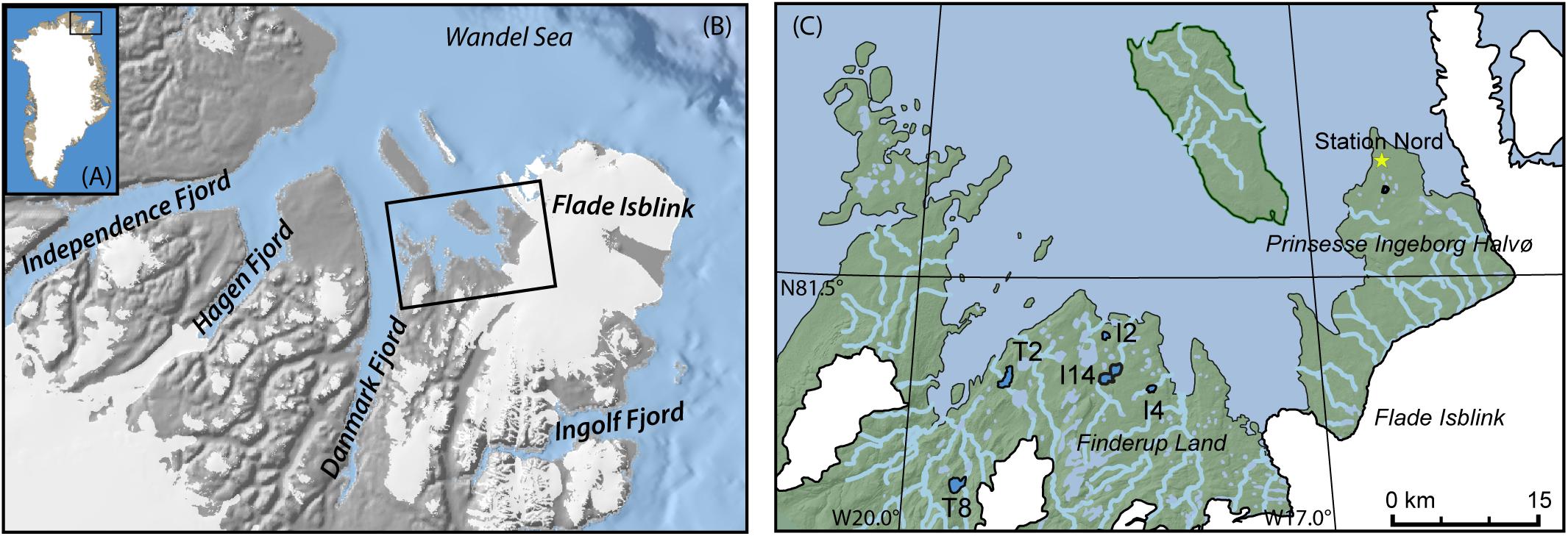
FIGURE 1. (A) Greenland with marked location of the larger area surrounding Finderup land shown in (B) (black box). (B) The larger area around Finderup Land with black box marking our field area as shown in detail in (C) (black box). (C) Map of Finderup Land with locations of cored isolation lakes from this study (numbered) and Sommersø, 4 km south of Station Nord, cored by Funder and Abrahamsen (1988).
During the Last Glacial Maximum (LGM), the ice sheet extended onto the shelf (Nørgaard-Pedersen et al., 2008; Larsen et al., 2010; Möller et al., 2010). It is, however, subject to debate whether the ice extended to the outer shelf (Jakobsson et al., 2014; Laberg et al., 2017) or had a more limited extent (Funder and Hansen, 1996; Funder et al., 2011b). The deglaciation history of Northeast Greenland indicates ice-free conditions in coastal areas between 11.8 and 9.0 ka (Bennike, 1987; Hjort, 1997; Bennike and Weidick, 2001; Bennike and Björck, 2002; Nørgaard-Pedersen et al., 2008; Funder et al., 2011b; Larsen et al., 2018). A slow, gradual RSL fall from ∼10.1 to ∼5.5 ka is described on the eastern side of Flade Isblink ice cap based on bivalve shells, driftwood, and a single whalebone (Bennike, 1997; Bennike and Weidick, 2001). The nearby area Prinsesse Ingeborg Halvø, 25 km northeast of Finderup Land (Figure 1B), experienced a slightly more accelerated RSL fall in the early Holocene and has a marine limit of c. 65 m a.s.l. based on bivalve shells, marine terraces, and one isolation lake (Funder and Abrahamsen, 1988; Funder et al., 2011a). A rapid sea level fall also took place from 9 to 6.5 ka in the area around Ingolf Fjord, ∼50 km southeast of Finderup Land (Hjort, 1997).
Materials and Methods
Sample Collection
We identified potentially suitable isolation lake basins using satellite imagery and aerial photographs at elevations ranging from present sea level to well above the approximate marine limit. Lake elevations were measured photogrammetrically in a pair of 1:150.000 scale aerial photographs from 1978. With stereo overlap, absolute vertical accuracies of ±1.0 m can be achieved (Kjeldsen et al., 2015). To get elevations in m a.s.l., we used the EGM2008 geoid, and calculate the elevations individually for each lake (Pavlis et al., 2012). In the field, we collected sediment cores from 5 lakes ranging in elevations from 19.6 to 81.2 m a.s.l. (Supplementary Table S1). We also attempted to retrieve cores from lakes at elevations between 0 and 19 m a.s.l., but were unsuccessful as these lakes were too shallow. We retrieved cores using a Tapper piston corer (Chambers and Cameron, 2001), using the frozen lake surface as our coring platform. We retrieved the cores from the lake center and measured water depth using a handheld echo sounder type Plastimo Echotest II. The cores were left to drain in upright position for at least 24 h after collection and were stored at 2–5°C. We split and cleaned the cores in the sediment laboratory at Aarhus University and then conducted lithological descriptions. The cores were subsequently photographed at high resolution and radiographic images were obtained using an ITRAX core scanner at the Aarhus University core scanning facility. The elemental composition was measured as counts per second (cps) at 1 mm intervals using a micro XRF sensor (Molybdenum tube), while magnetic susceptibility (MS) was measured using a Bartington MS2 sensor at 5 mm resolution with the ITRAX core scanner. Element counts are plotted with a 5-point moving average. We use MS, Ti and ratios of Ca/Fe and Sr/Ca as indicators of depositional environment. Ti is often associated with fine-grained, catchment-derived sediment input, which indicates terrigenous sediment sources and lacustrine conditions (Kylander et al., 2011; Croudace and Rothwell, 2015). Marine conditions are characterized by increased MS values, which reflects a relatively larger minerogenic sediment input and less biogenic (Sparrenbom et al., 2006a). Distinct changes in elemental composition reflect an environmental transition and ratios between elements are therefore commonly used to pinpoint the lake isolation (Sparrenbom et al., 2006a,b, 2013; Long et al., 2011; Larsen et al., 2016). Accordingly, marine conditions are characterized by a high Ca/Fe ratio and high MS, low Ti content and a low Sr/Ca ratio, whereas lacustrine conditions are characterized by higher Ti content, lower MS, low Ca/Fe ratio and high Sr/Ca ratio. We initially identified the marine/lacustrine transitions based on lithology, MS, and XRF data.
We furthermore subsampled for foraminiferal analyses, both for radiocarbon dating and for faunal evaluation, as foraminifera are excellent environmental indicators and their presence implies marine conditions. We searched for foraminifera in 1 cm increments in an interval 5–10 cm above and below the assumed marine to lacustrine transition in each core, as identified by the XRF data and lithology. Samples of ∼4 cm3 were weighed and wet sieved into grain size fractions of <63 μm, 63–100 μm, and >100 μm. Due to a relatively high content of clastic sand-sized sediment particles in some of the samples, the foraminiferal were concentrated by heavy liquid separation using tetrachlorethylene (C2Cl4) with a specific gravity of 1.6 g/cm3 prior to the faunal analysis. In most samples both the 63–100 μm and >100 μm fractions were analyzed for their foraminiferal content. When present, also the number of ostracod valves were counted.
Radiocarbon Dating
We sieved a large number of sediment samples from the cores in search for terrestrial macrofossils in order to radiocarbon date the transition from marine to lacustrine sediments. This was, however, unsuccessful probably due to the barren vegetation in the study area. We proceeded with dating bulk sediment samples, which was carried out at the Aarhus AMS Centre, Aarhus University, following the procedure of Brock et al. (2010). In addition, samples of mixed benthic foraminifera as well as a few containing both benthic foraminifera and ostracod valves were dated at the Ångström Laboratory, Uppsala University (Table 1). Radiocarbon ages were calibrated using OxCal 4.3 online (Ramsey, 2009) with the IntCal13 calibration curve for bulk samples and the Marine13 calibration curve for foraminifera (Reimer et al., 2013), with a marine reservoir effect of 550 14C a (ΔR = 150 14C a) (Mörner and Funder, 1990). Radiocarbon ages are given in cal ka BP while paleomagnetic correlated ages are given in ka (see below).
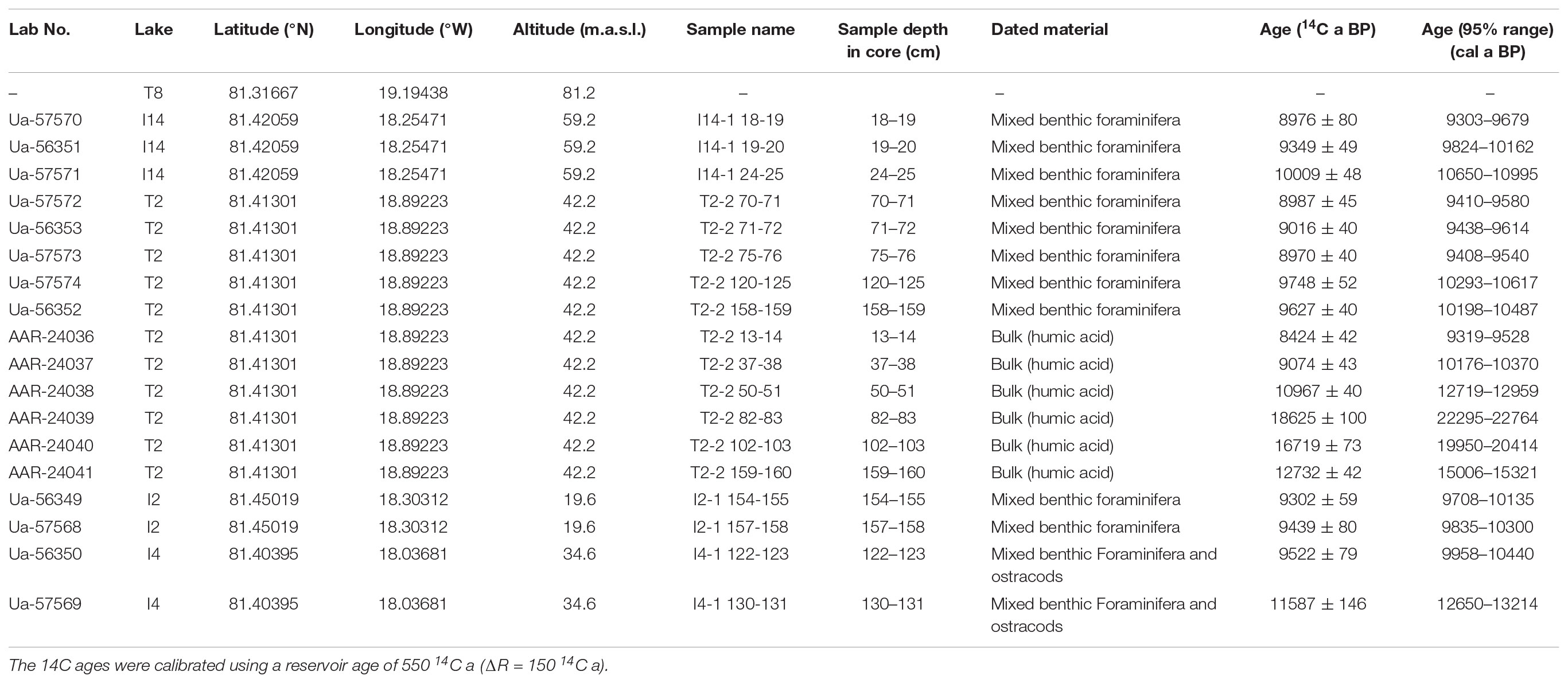
TABLE 1. Overview of investigated lakes, radiocarbon dates, dated material, and results.
Paleomagnetic Measurements and Age Correlation
Where possible, we constrain the age-depth chronology by correlation of paleomagnetic variations supported by radiocarbon dating of foraminifera. Paleomagnetic age reconstruction utilizes the secular variation of the Earth’s geomagnetic field, i.e., the slow variations in local geomagnetic field direction and intensity (Creer and Tucholka, 1983). During deposition, ferromagnetic sedimentary particles align with the ambient geomagnetic field and after a certain lock-in depth they will maintain their acquired orientation (Roberts et al., 2013). By measuring the inclination and declination recorded in the lakes in Finderup Land, and comparing the results to an independently dated reference curve, we are able to establish a chronology of the cores.
We collected discrete samples for every 2.5 cm in each core, using standard cubic paleomagnetic plastic boxes (2.2 × 2.2 × 2.2 cm) with an internal volume of 7 cm3. To isolate the ancient geomagnetic field signal, we measured the natural remanent magnetization (NRM) and the remaining remanent magnetization after stepwise demagnetizing the samples using alternating field (AF) with 10 milliTesla (mT) increments up to a maximum field strength of 80 mT. A viscous overprint was removed by AF demagnetization up to 10 mT and the characteristic remanent magnetization (ChRM) calculated using principal component analysis (Kirschvink, 1980). The maximum angular deviation (MAD) provides a measure of the precision with which the palaeomagnetic directions are determined, with values below 15° usually considered of acceptable quality (Butler, 1998). The median destructive field of the NRM, determined as the AF strength required to remove 50% of the initial magnetization, provides a measure of the coercivity (hardness) of the magnetic carrier. All measurements and analyses were carried out using a 2-G Enterprises model 755-R superconducting (DC SQUID) rock magnetometer at Lund University Paleomagnetic Laboratory.
We correlate our recorded paleomagnetic variations to three different reference curves; Global geomagnetic field model predictions for the site coordinates from (i) CALS10k.2 (Constable et al., 2016) and (ii) pfm9k.1a (Nilsson et al., 2014) that are both based on compilations of archaeomagnetic and sedimentary palaeomagnetic data. The models are valid to 10 and 9 ka respectively but we choose to show the full range of CALS10k.2, which extends to 12 ka but with only limited data support and with complications arising from spline end effects. In addition, we use the (iii) high-resolution Greenland/Iceland Composite (Stoner et al., 2013) which extends 11.5 ka and is compiled of two independently dated marine cores from the Denmark Strait. The Greenland/Iceland Composite data were relocated to the coordinates of Finderup Land assuming a dipole field, i.e., ‘conversion via pole’ (Noel and Batt, 1990). We note that due to the large distance between Finderup land and two marine cores (∼1500 km) there could be significant non-dipole field differences between the two sites that are not accounted for by this conversion. We then carried out a visual correlation of our measurements to the reference curves, constrained with radiocarbon ages from foraminifera.
Results and Interpretations
Lake T8
Lake T8 (informal name; N81.31667, W19.19438) is located at 81.2 m a.s.l., 5.5 km south of the coast and only 1.6 km west of the ice margin (Figure 1C). We retrieved a 104.5 cm core at a water depth of 18 m. We subdivide the core into two units (Figure 2); the lowermost unit (104.5–36 cm) consists of laminated silty clay with intervals of fine sand. Ti content and Sr/Ca ratio are low in this unit, while Ca/Fe is high. The uppermost unit has a base of clayey sand fining upward to silty clay. The XRF data show that the upper unit has high Ti content and high Sr/Ca ratio, while Ca/Fe ratio is low.
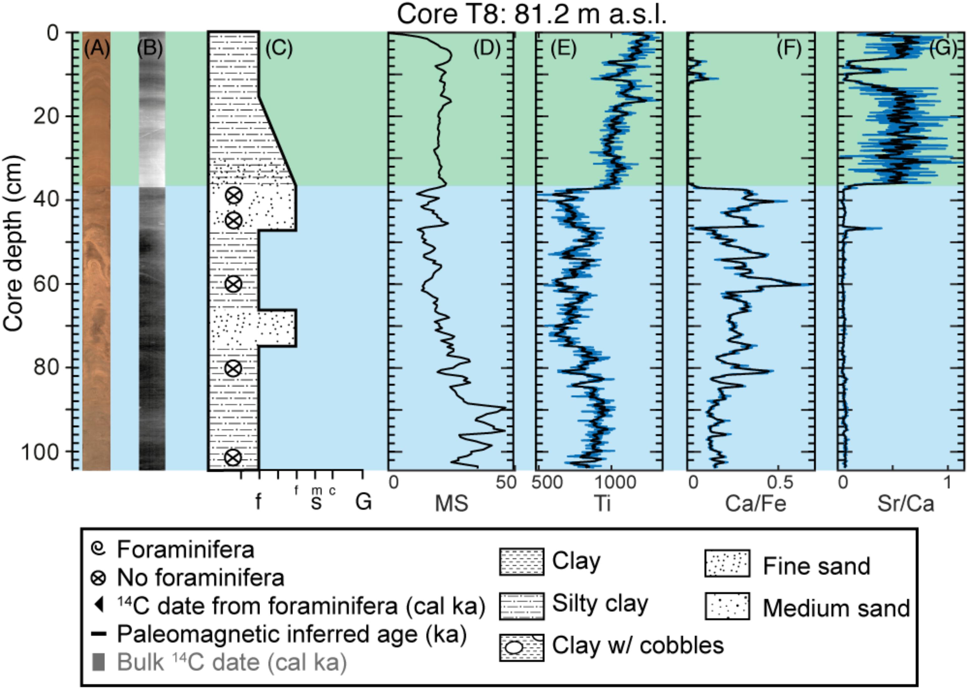
FIGURE 2. Overview of Core T8. (A) High-resolution image of the core. (B) X-ray image. (C) Lithologic log with grain sizes from fines (clay, silt) to sand and gravel. (D–G) Magnetic susceptibility measurement and content of Ti; Ca to Fe ratio; Sr to Ca ratio. Blue background color indicates marine conditions, green indicates lacustrine. Legend also applies to Figures 3, 4, 6, 7.
As seen from the elemental composition revealed by XRF core scanning, the transition between the two units is sharp and we interpret that the lowermost unit is deposited under marine conditions and the upper unit in a lacustrine environment, with the isolation of Lake T8 recorded at 36 cm. We searched the core for macrofossils and foraminifera but found neither. A paleomagnetic reconstruction was not possible for this core because of too-low declination values, most likely due to rotation of the coring instrument causing the core to be taken at an oblique angle. It has therefore not been possible to establish a chronology for the core from lake T8; however, the lake represents the highest observed isolation and is accordingly the minimum height of the marine limit for our field area.
Lake I14
Lake I14 (informal name; N81.42059, W18.25471) is located at 59.2 m a.s.l., 4.5 km south of the coastline and 10 km west of Flade Isblink (Figure 1C). We collected two cores close to each other from a water depth of 22 m. However, only one of these cores (I14-1) was dated and thus described here. The 78 cm long core can be subdivided into two units (Figure 3): The lower unit (78–18 cm) is initially dominated by pebbles to cobbles in a clayey-sandy matrix. This unit has a fining upward trend, and the top of the unit consists of gravel in a massive sandy matrix. Foraminifera are present in the uppermost part of the lower unit. The foraminiferal assemblage of I14-1 is dominated by large specimens of well-preserved Elphidium clavatum, and with Cassidulina reniforme, Buccella frigida, and Haynesina orbiculare as assesory species (Supplementary Table S2a. Foraminiferal counts for Core I14-2, also from Lake I14, are available in Supplementary Table S2b). Measurements of MS, along with Ca/Fe ratio are relatively high in the lowermost unit, whereas Ti content and Sr/Ca ratios are low. There is a sharp transition to the uppermost unit that consists of laminated silty clay with no foraminifera. In this unit, MS and Ca/Fe ratio are low, whereas Ti content and Sr/Ca are high.
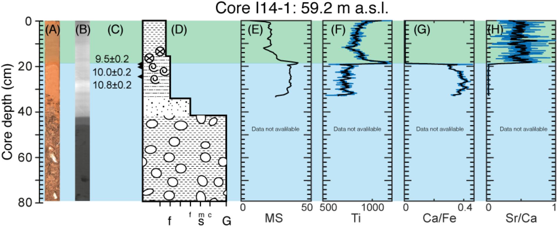
FIGURE 3. Overview of Core I14-1. (A) High-resolution image of the core. (B) X-ray image. (C) Age and position of radiocarbon dates from foraminifera (black triangles). (D) Lithologic log with grain sizes from fines (clay, silt) to sand and gravel. (E–H) Magnetic susceptibility measurement and content of Ti; Ca to Fe ratio; Sr to Ca ratio. Blue background color indicates marine conditions, green indicates lacustrine. Refer to Figure 2 for legend.
The foraminiferal assemblage in the top part of the marine interval of Core I14-1 indicates an Arctic fjord environment with reduced salinities. Based on lithology, foraminiferal presence and elemental composition, we thus interpret the lowermost unit as deposited under shallow-marine conditions, while the upper unit was deposited in a lacustrine environment, with the isolation of Lake I14 recorded at 18 cm.
We collected foraminifera for radiocarbon dates at three intervals from Core I14-1; (i) directly below the transition at 18–19 cm, which yielded an age of 9.5 ± 0.2 cal ka BP, (ii) at 19–20 cm, with an age of 10.0 ± 0.2 cal ka BP, and (iii) at 24-25 cm giving an age of 10.8 ± 0.2 cal ka BP (Table 1). Based on radiocarbon dates of foraminifera, Lake I14 represents a sea-level index point at 9.5 ± 0.2 cal ka BP.
Lake T2
Lake T2 (informal name; N81.41301, W18.89223) is located at an elevation of 42.2 m a.s.l., 1.5 km from the coast and 5 km from Flade Isblink (Figure 1C). We retrieved two almost identical sediment cores at a water depth of 6.5 m. Only core T2-2 is described here. The core is 161 cm long and has a uniform lithology consisting of laminated silty clay throughout the core (Figure 4). Core T2-2 can be subdivided into two units, based on XRF and microfossils; the lowermost unit (161-68 cm) has high MS values in the lower part, along with high Ca/Fe ratio. Ti content and Sr/Ca ratio are low in this unit. Foraminifera are abundant in several intervals of this lower unit, with the bottom intervals dominated by Elphidium clavatum with Elphidium asklundi and Buccella frigida as accessory species (Supplementary Table S3a. Foraminiferal counts for Core T2-1, also from Lake T2, are available in Supplementary Table S3b). Toward the top of the lower unit, the assemblage in Core T2-2 becomes fairly diverse and characterized by Elphidium clavatum, Elphidium asklundi, Buccella frigida, Cassidulina reniforme and Eoeponidella pulchella, with Haynesina nivea, Stainforthia loeblichi, and A. gallowayi as accessory species. The presence of planktonic foraminiferal is noteworthy. Presence of foraminifera concludes abruptly at the top of the lowermost unit. The upper unit (68-0 cm) has relatively low MS and low Ca/Fe ratio. Ti content along with Sr/Ca ratio is high in the uppermost unit, and foraminifera are not present. The transition between the two units is sharp.
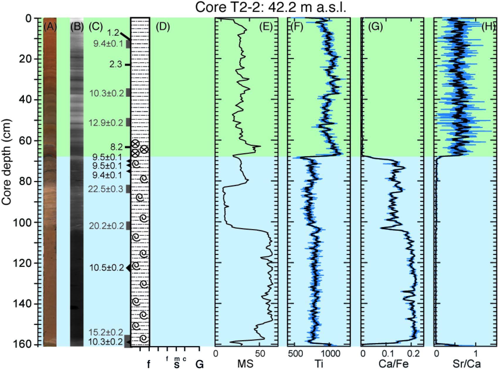
FIGURE 4. Overview of Core T2-2. (A) High-resolution image of the core. (B) X-ray image. (C) Age and position of radiocarbon dates from foraminifera (black triangles) and ages inferred from paleomagnetic correlation (black lines). Gray boxes and gray text denote ages from bulk radiocarbon dating. (D) Lithologic log with grain sizes from fines (clay, silt) to sand and gravel. (E–H) Magnetic susceptibility measurement and content of Ti; Ca to Fe ratio; Sr to Ca ratio. Blue background color indicates marine conditions, green indicates lacustrine. Refer to Figure 2 for legend.
Based on the elemental composition and presence of a diverse foraminiferal assemblage, we interpret that the lowermost unit was deposited under near-normal marine salinities in an Arctic inner shelf to fjord environment (Hald and Korsun, 1997). The presence of high-productivity indicators such as Buccella frigida, Eoeponidella pulchella, Haynesina nivea, and Stainforthis loeblichi may be linked to sea-ice marginal (Seidenkrantz, 2013). The lower part of the marine core interval contains numerous planktonic foraminifera, including several species today linked to relatively warm waters (Schiebel and Hemleben, 2017). This indicates influx of marine waters of Atlantic source as seen in the deeper sites of Independence Fjord today (Dmitrenko et al., 2017), also clearly impacting the marine habitats of the fjord system (Limoges et al., 2018). We interpret the upper unit (68-0 cm) to represent a lacustrine environment, with the isolation of Lake T2 recorded at 68 cm.
We dated foraminifera at five intervals between 159 and 70 cm, as summarized in Table 1, and the results consistently point to a high deposition rate in the marine core interval. An attempt was made at radiocarbon dating of the humic acid fraction of bulk sediment samples at several intervals in the core from Lake T2. The bulk samples gave ages ranging from 9.3 cal ka BP near the top of the core to 22.8 cal ka BP toward the middle of the core (Table 1 and Figure 4). These dates are clearly too high due to old organic material adhering to the sediment grains or to mobilization of old carbon in the catchment area, which affects the measured 14C age (Olsen et al., 2011).
Core T2-2 showed suitable mineral magnetic grain properties for a paleomagnetic age correlation. NRM intensities range from 3 to 120 mAm-1 and are almost completely removed after 80 mT AF demagnetization, with MDFs of 27-44 mT (Supplementary Figure S1). The ChRM, isolated between 10 and 80 mT, shows a single stable component with MAD values below 3.5°. The demagnetization data from a typical sample of Core T2-2 is shown in Supplementary Figure S3A. Based on the constraints provided by the five radiocarbon dates and visual correlation of both inclination and declination to the CALS10k.2 model prediction (Constable et al., 2016) we identified three palaeomagnetic tie-points at 11, 23.5, and 63 cm depth (Figure 5). The resulting age-depth model (Figure 5) places the isolation of Lake T2 at 9.1 ka.
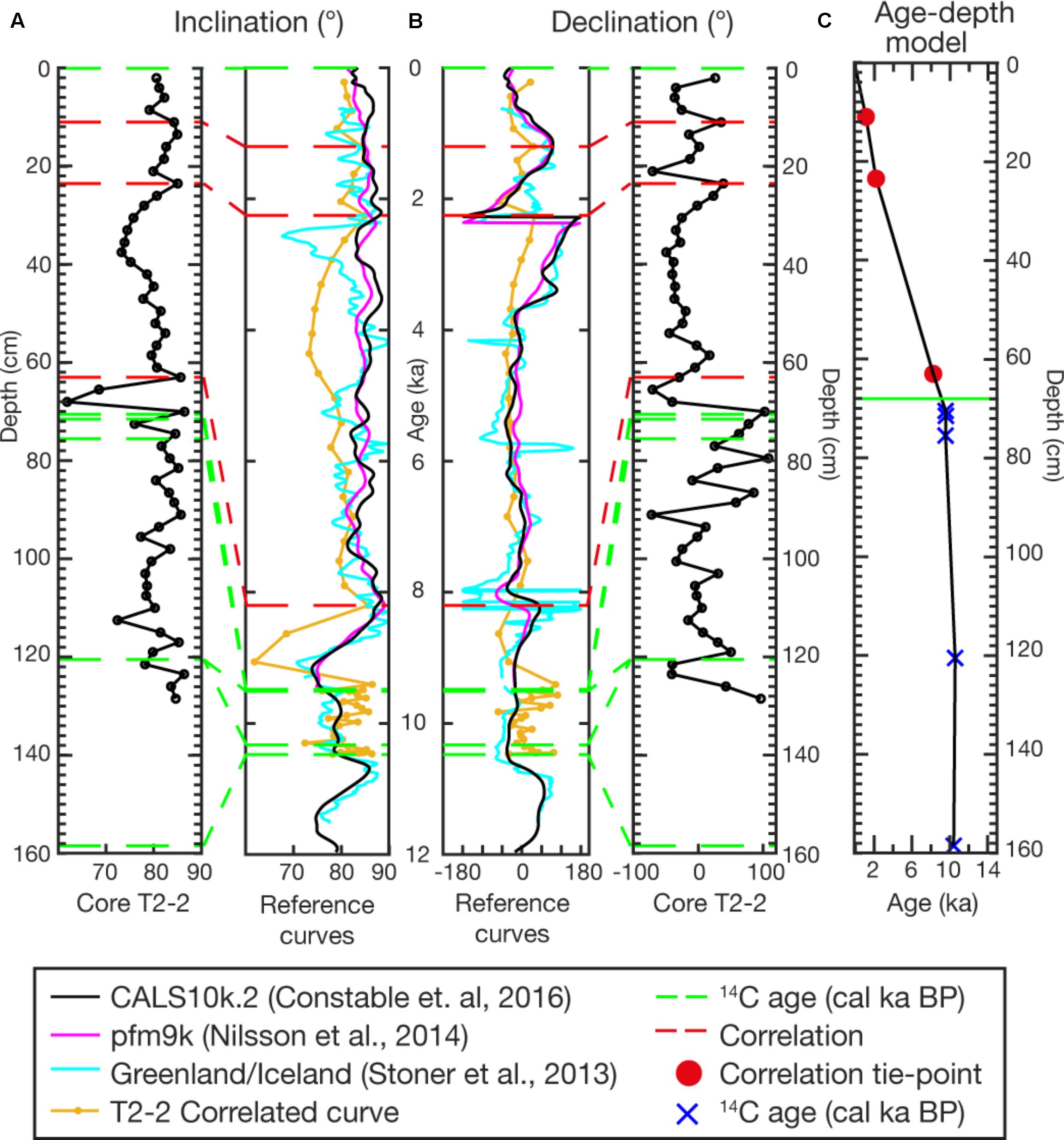
FIGURE 5. Correlation of paleomagnetic measurements of (A) inclination and (B) declination in Core T2-2 to three reference curves (see Legend). Stippled lines indicate correlation points. Green stippled lines are constraints based on 14C ages. The resulting age-depth model for core T2-2 is shown in (C).
Lake I4
Lake I4 (informal name; N81.40395, W18.03681) is situated at 34.6 m a.s.l., 1.5 km from the coast and 11–12 km from the nearest lobes of Flade Isblink (Figure 1C). We retrieved a 161 cm long core at 20 m water depth. The sediments are composed of laminated silty clay with intervals of laminated clay toward the top. Again, the core can be divided into two units (Figure 6); the lowermost part has relatively low Ti content, high Ca/Fe ratio and low Ca/Sr ratio. Foraminifera are present in the lower unit; the assemblage is dominated by Elphidium clavatum with Buccella frigida and Cassiduina reniforme as accessory species (Supplementary Table S4). It was possible to gather enough individual foraminifera for radiocarbon dates at 130–131 cm and 122–123 cm. Above 122 cm, foraminifera abundance decreases until they completely disappear at 117 cm. The upper unit is characterized by absence of foraminifera, a slight increase in Ti content and an increase in Sr/Ca ratio, along with a marked drop in Ca/Fe ratio. Plant macrofossils are absent throughout the core.
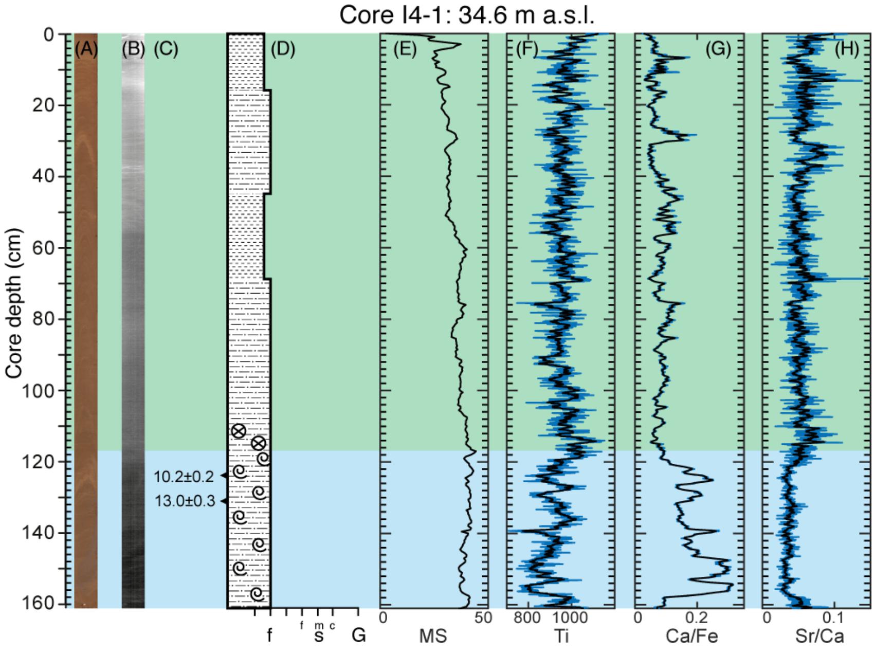
FIGURE 6. Overview of Core I4-1. (A) High-resolution image of the core. (B) X-ray image. (C) Age and position of radiocarbon dates from foraminifera (black triangles). (D) Lithologic log with grain sizes from fines (clay, silt) to sand and gravel. (E–H) Magnetic susceptibility measurement and content of Ti; Ca to Fe ratio; Sr to Ca ratio. Blue background color indicates marine conditions, green indicates lacustrine. Refer to Figure 2 for legend.
The assemblage of foraminifera in the lowermost unit indicates an Arctic, fairly shallow-water environment with somewhat reduced salinities and a high-productivity, which often occurs under sea-ice conditions (Hald and Korsun, 1997; Seidenkrantz, 2013). The drop in abundance coincides with a transition to the upper unit seen from XRF cm and we interpret the marine to lacustrine transition to be at the division between the two units, at 117 cm.
Radiocarbon dating of foraminifera from 130–131 cm yielded an age of 13.0 ± 0.3 cal ka BP and from 122–123 cm an age of 10.2 ± 0.2 cal ka BP (Table 1). A paleomagnetic age correlation was not possible, unfortunately. The core showed acceptable magnetic grain properties, however, the resulting paleomagnetic measurements from the core did not bear any fluctuations that were recognizable in the master core. Consequently, we were not able to date the isolation of Lake I4, but only to establish a maximum age of 10.2 ± 0.2 cal ka BP.
Lake I2
Lake I2 (informal name; N81.45019, W18.30312) is located at 19.6 m a.s.l., 650 m from the coast and 12.5 km from Flade Isblink (Figure 1C). The surrounding terrain consists of shallow undulating hills and the lake drains to the sea by a stream that flows to the northeast (Figure 1C). We retrieved a 158.5 cm long core at 7 m water depth (I2-1). The core can be subdivided into two units using the XRF data, as both units consist of laminated silty clay (Figure 7). The lower unit is characterized by an increased Ca/Fe ratio along with a low Sr/Ca ratio. MS is high in the lowermost core part and decreases gradually from 132 cm and upward. The upper unit has low MS values, while the Ca/Fe ratio is at first consistently low, but then becomes more variable for the upper 70 cm. The Sr/Ca ratio is initially steeply increased in the uppermost core unit before it decreases at ∼70 cm core depth. The Ti content is not markedly different between the two units. There are no plant macrofossils present in the core. Foraminifera were found in the bottommost parts of the core from 158 to 152 cm, where the assemblage was dominated by Elphidium clavatum and Cassidulina reniforme, which are species commonly found in Arctic and subarctic environments (Hald et al., 1994; Hald and Korsun, 1997; Jennings et al., 2004), including in the present Independence Fjord (Limoges et al., 2018). The increase in Elphidium albiumbilicatum and Elphidium bartletti upward in the core indicates reduced salinities (cf. Polyak et al., 2002) followed by a decrease in abundance, indicating a gradual shallowing from 154–152 cm before the foraminifera disappear at 152 cm (Supplementary Table S5. For a list of all foraminiferal species found in this study, see Supplementary Table S6).
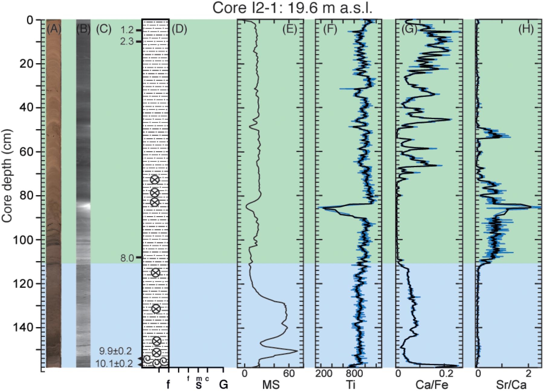
FIGURE 7. Overview of Core I2-1. (A) High-resolution image of the core. (B) X-ray image. (C) Age and position of radiocarbon dates from foraminifera (black triangles) and ages inferred from paleomagnetic correlation (black lines). (D) Lithologic log with grain sizes from fines (clay, silt) to sand and gravel. (E–H) Magnetic susceptibility measurement and content of Ti; Ca to Fe ratio; Sr to Ca ratio. Blue background color indicates marine conditions, green indicates lacustrine. Refer to Figure 2 for legend.
Based on the XRF elemental composition measurements and benthic foraminiferal faunas, we interpret that the lowermost unit is deposited under marine, upward-shallowing conditions and the upper unit in a lacustrine environment. The constant Ti content throughout the core suggests that the basin has had continuous sediment influx from terrigenous sources and that the exchange with the open ocean has been insufficient in balancing this influx. The early decrease in MS likely reflects a gradual cut-off of the basin’s connection with the open ocean, which corresponds to the foraminiferal analyses indicating gradual shallowing. There is, however, a clear environmental transition seen from Ca/Fe and Sr/Ca ratios showing the final lake isolation at 110 cm. There were no appearances of foraminifera above 110 cm. We were not able to fully resolve the scatter in Ca/Fe and the decrease in Sr/Ca in the uppermost core intervals, however, we find it highly unlikely that it should suggest reestablishment of marine conditions, as the lake is presently at 19.6 m a.s.l. and marine conditions in the upper part of the core would therefore imply an extreme uplift in the Late Holocene.
We collected foraminifera for radiocarbon dating at 154–155 cm, which yielded an age of 9.9 ± 0.2 cal ka BP and at 157–158 cm, giving an age of 10.1 ± 0.2 cal ka BP (Table 1). Paleomagnetic measurements showed suitable mineral magnetic grain properties for age correlation. NRM intensities range from 1 to 74 mAm-1 with MDFs of 20–52 mT (Supplementary Figure S2). The Zijderveld plots typically show a single component demagnetizing toward the origin (Supplementary Figure S3B) apart from a short interval, between 108 and 125 cm, that appear to acquire a gyroremanent magnetization (GRM) (Snowball, 1997) at high AF demagnetization fields (Supplementary Figure S3C). GRMs are indicative of authigenic greigite that grows in reducing conditions (Roberts et al., 2011; Nilsson et al., 2013), often accompanied by magnetite dissolution that could explain the low NRM intensities over the same interval. The ChRMs were isolated between 10 and 80 mT, except for the short interval 108–125 cm where we used 10-50 mT to minimize the effects of the GRM acquisition, with MAD values generally below 5°. However, the directions from the interval with suspected greigite should be viewed with caution as the timing of the remanent magnetization (and growth of the mineral) would then be unknown.
The generally suitable mineral magnetic grain properties allowed us to do a visual correlation (Figure 8) to the CALS10k.2 reference curve (Constable et al., 2016). Based on the constraints provided by two radiocarbon dates from foraminifera (see above) we identified three palaeomagnetic tie-points at 4.5, 9.5, and 108 cm. The resulting age-depth model of the core (Figure 8) places the timing of isolation of Lake I2 at 8.0 ka.
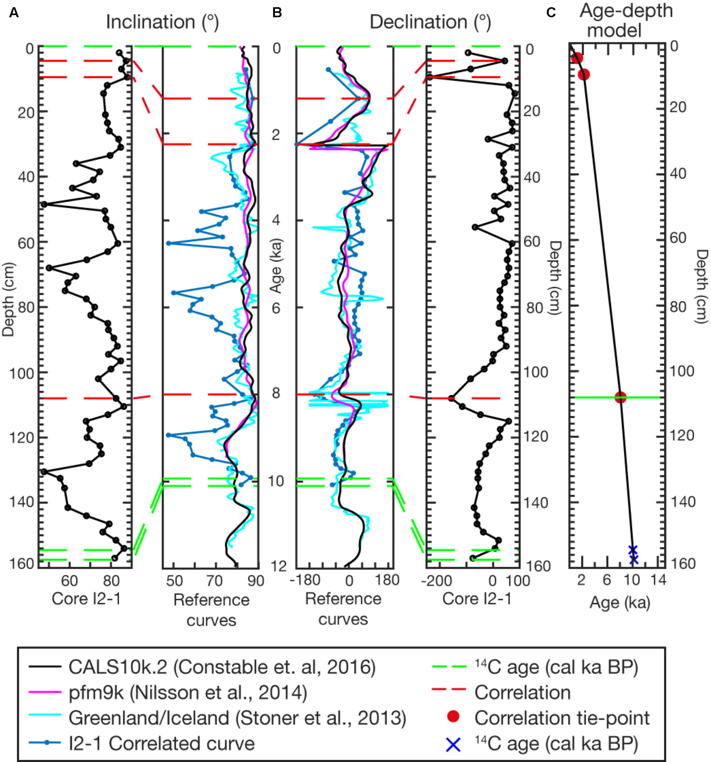
FIGURE 8. Correlation of paleomagnetic measurements of (A) inclination and (B) declination in Core I2-1 to three reference curves (see Legend). Stippled lines indicate correlation points. Green stippled lines are constraints based on 14C ages. The resulting age-depth model for core I2 is shown in (C).
Discussion
Relative Sea Level Reconstruction
We identify and date the transition from marine to lacustrine depositional environments in four North Greenland lakes (I2, I4, I14, and T2). We furthermore show that the marine limit in Finderup Land is at least 81.2 m above present sea level, as marine sediment is present in Lake T8 at this elevation. The marine limit could potentially be even higher. However, our data cannot resolve this, as we did not investigate lakes above 81.2 m a.s.l. Based on the four sea-level index points we establish a RSL curve for Finderup Land (Figure 9A). The course of the RSL curve above Lake I14 at 59.2 m a.s.l. remains unknown as we were not able to date Lake T8 at 81.2 m a.s.l. We therefore illustrate two possible scenarios with varying rates of early RSL fall from 81.2–59.2 m a.s.l. In one scenario, the steep RSL fall is continued from 9.5 ka and back in time, which implies a late onset of the deglaciation and an extremely fast ice retreat. In the second scenario, the RSL rate of change is decreased from 9.5 to 10.8 ka. The second scenario is likely more realistic, as we know Finderup Land was submerged by 10.8 ka, and perhaps earlier, as foraminifera were present at this time in Lake I14.
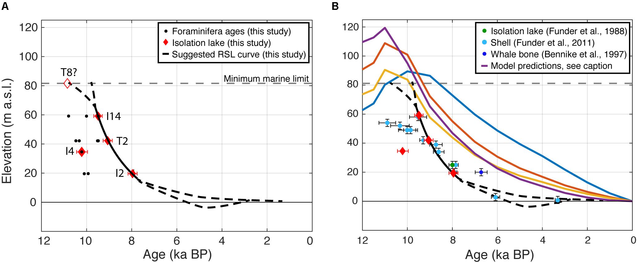
FIGURE 9. (A) Relative sea level data for Finderup Land with foraminifera ages (black dots) and isolation lakes (red diamonds). The black line shows the, suggested relative sea level curve based on the data presented here. (B) Data from this study presented together with findings from Funder and Abrahamsen (1988); Bennike (1997), and Funder et al. (2011a). Driftwood data from Funder et al. (2011a) was omitted in this plot because it had large scatter. Solid colored lines show predicted RSL by various models. Orange: Huy2 (Simpson et al., 2009). Yellow: Huy3 (Lecavalier et al., 2014). Blue: ICE-5G (Peltier, 2004). Purple: Huy3 NGr variant (Lecavalier et al., 2017).
The index point from Lake I4 falls below the curve and we suspect that this age does not represent the time of deposition, but rather can be explained by redeposition of older marine sediment washed into the basin. Neither the foraminiferal nor the ostracod specimens that were dated showed any significant abrasion or signs of re-working. However, reworking cannot always easily be detected, as foraminiferal may be transported as sand-sized particles (Boltovskoy and Wright, 1976). It is, however noteworthy that Core I4-1 was the only one where we used a mix of benthic foraminifera and ostracod valves for dating.
Our data imply rapid emergence of the area with an RSL fall of 2.6 cm a-1 from 9.5 ± 0.2 cal ka BP to 8.0 ka, at which point the RSL begins to approach present sea level. The RSL history from 8.0 ka BP to present remains unresolved, however, several studies from North and Northeast Greenland indicate that the ice retreated behind its current margins and readvanced during the Neoglacial (Weidick et al., 1996; Bennike and Weidick, 2001; Funder et al., 2011b; Larsen et al., 2018). We therefore consider the possibility of sea level falling below 0 m a.s.l. before rising to its present level (Figures 9A,B). This hypothesis can be investigated further by retrieving marine sediment cores close to the coast off of Finderup Land.
Comparison to Existing Geological Data
Our results constitute the first RSL curve from North and Northeast Greenland based on isolation lakes. Previous studies construct a RSL curve for Prinsesse Ingeborg Halvø based on a compilation of samples of driftwood and bivalve shells as well as one isolation lake at 25 m a.s.l. with an age of 8.0 ± 0.1 cal ka BP (Funder and Abrahamsen, 1988; Funder et al., 2011a). These data points generally fall along the same curve as suggested by the isolation lakes from Finderup Land. This is surprising as bivalve shells and driftwood often are more scattered in age and relative to the shoreline than isolation lakes (Figure 9B). Additionally, a whale skeleton was found in Prinsesse Ingeborg Halvø with an age of 6.7 ± 0.3 cal ka BP (Bennike, 1997), placing it just above the curve described by our data, where it most likely stranded just above sea level. On a larger regional scale, the few available RSL curves agree with a steep RSL decline from ∼11 cal ka BP to ∼8 cal ka BP in North (England, 1985; Funder and Abrahamsen, 1988; Kelly and Bennike, 1992; Hjort, 1997) and Northeast Greenland (Wagner and Melles, 2002; Hall et al., 2010). This steep RSL decline can be explained by a consistently rapid ice retreat in North and Northeast Greenland that coincides with the noticeable temperature increase in the same period (Lecavalier et al., 2017).
Our data reveal that Finderup Land was deglaciated by at least 10.8 ± 0.2 cal ka BP, at which time the ocean had already inundated Lake I14. Deglaciation most likely occurred earlier in the region, as we found marine sediments 22 m above Lake I14, in Lake T8, therefore we use 10.8 ± 0.2 cal ka BP as a minimum-limiting age for deglaciation of the region. Unfortunately, we do not have a chronology on Lake T8 to further constrain the timing of deglaciation. Ice-free conditions at 10.8 ± 0.2 cal ka BP occur slightly earlier than findings from the nearby areas surrounding Independence Fjord, which indicate deglaciation by ∼10.0 cal ka BP (Bennike, 1987; Bennike and Björck, 2002; Nørgaard-Pedersen et al., 2008).
Comparison to Modeled Predictions
Several GIA models estimate the RSL through the last 12 ka and find different possible scenarios depending on ice sheet extent at the LGM, type of ice sheet model, temperature forcing, and lithosphere model configurations. We compare our data to four models and find that the regression in Finderup Land occurred faster and earlier than all of the predicted scenarios (Figure 9B). The largest data-model misfit is to the prediction made by the GrB model (Peltier, 2004), most likely due to an underestimate of ice load resulting from inadequate RSL data availability when the ice sheet model was devised. RSL data are essential constraints for calibration of ice sheet models, which explains why the proceeding three predictions have a much smaller data-model misfit. Correspondingly, the Huy2 model (Simpson et al., 2009) provides a closer fit, being constrained by a larger number of RSL observations in addition to field data on former ice margin position. In this model the ice sheet is allowed to extend far out on the continental shelf in Northeast Greenland, as suggested by Nørgaard-Pedersen et al. (2008) and Laberg et al. (2017), and the LGM ice sheet thickness is estimated to an excess of 4.1 m ice-equivalent sea level (IESL) relative to present (Simpson et al., 2009).
Being based on a more extensive constraint database, the Huy3 model (Lecavalier et al., 2014) and the Huy3 Ngr variant (Lecavalier et al., 2017) formulate closest model-data fit. The Huy3 is a uniform model for all of Greenland, using a temperature reconstruction based on the GRIP δ18O record (Dansgaard et al., 1993), whereas the Huy3 Ngr variant is a regional model for Northwest Greenland that takes account of enhanced influence from the North American ice complex and is based on the recent temperature reconstruction from the Agassiz ice cap (Lecavalier et al., 2017). Both Huy3 models have a thicker and more extensive ice sheet than their predecessors, as they reach further onto the shelf and describe the LGM thickness with an excess of 4.7 m IESL relative to present (Lecavalier et al., 2014). As our suggested RSL curve falls below the curves predicted by both Huy3 models (Figure 9B), we suggest that the ice sheet may have been thicker and perhaps more extensive than suggested by both models.
Implications for the Ice Sheet History of North Greenland in the Late Quaternary
Our data support the notion of a bigger ice loading, i.e., an ice sheet that extended far out onto the shelf and most likely was thicker than predicted by the available models. The Finderup Land isolation lakes reveal an RSL curve that responds to a faster and earlier uplift than captured by any of the models, however, the closest fit is achieved by the models with the thickest and most extensive ice sheet (Lecavalier et al., 2014, 2017). The fast isostatic uplift of Finderup Land is likely a result of rapid ice retreat in the major fjord systems (Independence Fjord, Hagen Fjord, and Danmark Fjord), which would serve as a gateway for increased calving during the deglaciation. The early Holocene diminution of the GrIS coincides with a distinct surface temperature increase recorded in Agassiz ice core (Lecavalier et al., 2017) as well as general Greenland-wide warming (Buizert et al., 2018). In addition, the Fram Strait was dominated by warm water in this period (Werner et al., 2016) and sea ice cover shifted from permanent to seasonal (Müller et al., 2009). All of these factors would increase the rate of deglaciation during the early Holocene and consequently, cause an accelerated isostatic uplift.
Conclusion
In this study, we reconstructed RSL fluctuations since deglaciation in Finderup Land, North Greenland using sediment cores from five isolation lakes, which yield accurate and precise sea level index points. We established a marine limit at minimum 81.2 m a.s.l. and conclude that Finderup Land was ice free by at least 10.8 ± 0.2 cal ka BP. Our data show a rapid RSL fall from 9.5 ± 0.2 cal ka BP to 8.0 ka, at which point the RSL began to approach present sea level. The RSL history from 8.0 ka until present remains unresolved, and RSL can have fallen below present level due to significant ice retreat during the Holocene Thermal Maximum followed by Neoglacial ice advance. We compared our data to GIA models and found that the best model-data match was achieved by the Huy3 model (Lecavalier et al., 2014) and the Huy3 Ngr variant model (Lecavalier et al., 2017), which are initialized with a thick ice sheet extending far out onto the shelf edge in North and Northeast Greenland. Our data indicate that the GrIS was even thicker and also, potentially, more extensive than estimated by both models, and that the post LGM ice loss was, therefore, larger than previously anticipated.
Author Contributions
NL conceived the research. AS, LL, NL, and TL conducted the fieldwork in 2015. AS and JO prepared samples for bulk 14C dating and JO measured 14C concentrations on AMS. M-SS performed foraminiferal analyses and interpretations. AS and AN performed paleomagnetic analyses and interpretations. AS wrote main manuscript with assistance from all authors.
Funding
The field work forming the basis of this study was supported by Arctic Research Centre (ARC), Aarhus University. NL was supported by the Villum Young Investigator Programme and M-SS was supported by the Independent Research Fund Denmark (G-Ice project Grant No. 7014-00113B/FNU).
Conflict of Interest Statement
The authors declare that the research was conducted in the absence of any commercial or financial relationships that could be construed as a potential conflict of interest.
Acknowledgments
We thank Bjarki Friis and Ivali Lennert for their support during fieldwork and Pernille Bülow is thanked for her assistance with laboratory processing of samples.
Supplementary Material
The Supplementary Material for this article can be found online at: https://www.frontiersin.org/articles/10.3389/feart.2018.00129/full#supplementary-material
References
Bengaard, H. J., and Henriksen, N. (1986). Geological Map of Greenland, 1:500 000. Peary Land: Geological Survey of Greenland.
Bennike, O. (1987). Quaternary geology and biology of the Jørgen Brønlund Fjord area, North Greenland. Geoscience 18, 1–24.
Bennike, O. (1997). Quaternary vertebrates from Greenland: a review. Quat. Sci. Rev. 16, 899–909. doi: 10.1016/S0277-3791(97)00002-4
Bennike, O., and Björck, S. (2002). Chronology of the last recession of the Greenland Ice Sheet. J. Quat. Sci. 17, 211–219. doi: 10.1002/jqs.670
Bennike, O., Björck, S., and Lambeck, K. (2002). Estimates of South Greenland late-glacial ice limits from a new relative sea level curve. Earth Planet. Sci. Lett. 197, 171–186. doi: 10.1016/S0012-821X(02)00478-8
Bennike, O., and Weidick, A. (2001). Late quaternary history around nioghalvfjerdsfjorden and Jøkelbugten, North-East Greenland. Boreas 30, 205–227. doi: 10.1111/j.1502-3885.2001.tb01223.x
Boltovskoy, E., and Wright, R. (1976). Recent Foraminifera. The Hague: Dr. W Junk b.v., 514. doi: 10.1007/978-94-117-28507
Brock, F., Higham, T., Ditchfield, P., and Ramsey, C. B. (2010). Current pretreatment methods for AMS radiocarbon dating at the oxford radiocarbon accelerator unit (ORAU). Radiocarbon 52, 103–112. doi: 10.2458/azu_js_rc.52.3240
Buizert, C., Keisling, B. A., Box, J. E., He, F., Carlson, A. E., Sinclair, G., et al. (2018). Greenland-wide seasonal temperatures during the last deglaciation. Geophys. Res. Lett. 45, 1905–1914. doi: 10.1002/2017GL075601
Butler, R. F. (1998). Magnetic Domains to Geologic Terranes, Electronic Edn. Oregon: Department of Chemistry and Physics, University of Portland.
Chambers, J. W., and Cameron, N. (2001). A rod-less piston corer for lake sediments: an improved, rope-operated percussion corer. J. Paleolimnil. 25, 117–122. doi: 10.1023/A:1008181406301
Church, J. A., Clark, P. U., Cazenave, A., Gregory, J. M., Jevrejeva, S., Levermann, A., et al. (2013). “Sea level change,” in Climate Change 2013: The Physical Science Basis. Contribution of Working Group I to the Fifth Assessment Report of the Intergovernmental Panel on Climate Change, eds T. F. Stocker et al. (Cambridge: Cambridge University Press).
Constable, C., Korte, M., and Panovska, S. (2016). Persistent high paleosecular variation activity in southern hemisphere for at least 10000 years. Earth Planet. Sci. Lett. 453, 78–86. doi: 10.1016/j.epsl.2016.08.015
Creer, K. M., and Tucholka, P. (1983). On the current state of lake sediment palaeomagnetic research. Geophys. J. Int. 74, 223–238. doi: 10.1111/j.1365-246X.1983.tb01878.x
Croudace, I. W., and Rothwell, R. G. (2015). “Micro-XRF studies of sediment cores: applications of a non-destructive tool for the environmental sciences,” in Developments in Paleoenvironmental Research, Vol. 17, ed. J. P. Smol (Heidelberg: Springer), doi: 10.1007/978-94-017-9849-5.
Dansgaard, W., Johnsen, S. J., Clausen, H. B., Dahl-Jensen, D., Gundestrup, N. S., Hammer, C. U., et al. (1993). Evidence for general instability of past climate from a 250-kyr ice-core record. Nature 364, 218–220. doi: 10.1038/364218a0
Dmitrenko, I. A., Kirillov, S. A., Rudels, B., Babb, D. G., Pedersen, L. T., Rysgaard, S., et al. (2017). Arctic Ocean outflow and glacier-ocean interaction modify water over the Wandel Sea shelf, northeast Greenland. Ocean Sci. 13, 1045–1060. doi: 10.5194/os-2017-28
Dutton, A., Carlson, A. E., Long, A. J., Milne, G. A., Clark, P. U., DeConto, R., et al. (2015). Sea-level rise due to polar ice-sheet mass loss during past warm periods. Science 349:aaa4019. doi: 10.1126/science.aaa4019
England, J. (1985). The late quaternary history of hall land, northwest Greenland. Can. J. Earth Sci. 22, 1394–1408. doi: 10.1139/e85-147
Funder, S. (1989). “Quaternary geology of the ice-free areas and adjacent shelves of Greenland,” in Quaternary Geology of Canada and Greenland Geological Survey of Canada, (Geology of Canada Vol. 1), ed. R. J. Fulton (Ottawa: Geological Society of America), 741–792.
Funder, S., and Abrahamsen, N. (1988). Palynology in a polar desert, eastern North Greenland. Boreas 17, 195–207. doi: 10.1111/j.1502-3885.1988.tb00546.x
Funder, S., Goosse, H., Jepsen, H., Kaas, E., Kjær, K. H., Korsgaard, N. J., et al. (2011a). A 10,000-year record of arctic ocean sea-ice variability—view from the beach. Science 333, 747–751. doi: 10.1126/science.1202760
Funder, S., Kjeldsen, K. K., Kjær, K. H., and Cofaigh, C. Ó (2011b). “The Greenland Ice Sheet during the past 300,000 years: a review,” in Developments in Quaternary Sciences, eds J. Ehlers, P. Gibbard, and P. D. Hughes (Amsterdam: Elsevier), 699–713. doi: 10.1016/B978-0-444-53447-7.00050-7
Funder, S., and Hansen, L. (1996). The Greenland ice sheet - a model for its culmination and decay during and after the last glacial maximum. Bull. Geol. Soc. Denmark 42, 137–152.
Gregory, J. M., White, N. J., Church, J. A., Bierkens, M. F. P., Box, J. E., van den Broeke, M. R., et al. (2013). Twentieth-century global-mean sea level rise: is the whole greater than the sum of the parts? J. Clim. 26, 4476–4499. doi: 10.1175/JCLI-D-12-00319.1
Hald, M., Dokken, T., Korsun, S., Polyak, L., and Aspeli, R. (1994). Recent and Late quaternary distribution of Elphidium excavatum f. clavata in Arctic seas. Cushman Found. Spec. Publ. 32, 141–153.
Hald, M., and Korsun, S. (1997). Distribution of modern benthic foraminifera from fjords of Svalbard, European Arctic. J. Foraminifera Res. 27, 101–122. doi: 10.2113/gsjfr.27.2.101
Hall, B. L., Baroni, C., and Denton, G. H. (2010). Relative sea-level changes, schuchert Dal, East Greenland, with implications for ice extent in late-glacial and Holocene times. Quat. Sci. Rev. 29, 3370–3378. doi: 10.1016/j.quascirev.2010.03.013
Hay, C., Mitrovica, J. X., Gomez, N., Creveling, J. R., Austermann, J. E., and Kopp, R. (2014). The sea-level fingerprints of ice-sheet collapse during interglacial periods. Quat. Sci. Rev. 87, 60–69. doi: 10.1016/j.quascirev.2013.12.022
Hjort, C. (1997). Glaciation, climate history, changing marine levels and the evolution of the Northeast Water Polynya. J. Mar. Syst. 10, 23–33. doi: 10.1016/S0924-7963(96)00068-1
Jakobsson, M., Andreassen, K., Bjarnadóttir, L. R., Dove, D., Dowdeswell, J. A., England, J. H., et al. (2014). Arctic ocean glacial history. Quat. Sci. Rev. 92, 40–67. doi: 10.1016/j.quascirev.2013.07.033
Jennings, A. E., Weiner, N. J., Helgadottir, G., and Andrews, J. T. (2004). Modern foraminiferal faunas of the southwestern to Northern Iceland shelf: oceanographic and environmental controls. J. Foraminiferal Res. 34, 180–207. doi: 10.2113/34.3.180
Kelly, M., and Bennike, O. (1992). Quaternary geology of western and central North Greenland. Rapport Grønlands Geologiske Undersøgelse 153:34.
Kirschvink, J. L. (1980). The least-squares line and plane and the analysis of palaeomagnetic data. Geophys. J. Int. 62, 699–718. doi: 10.1111/j.1365-246X.1980.tb02601.x
Kjeldsen, K. K., Korsgaard, N. J., Bjørk, A. A., Khan, S. A., Box, J. E., Funder, S., et al. (2015). Spatial and temporal distribution of mass loss from the Greenland Ice Sheet since AD 1900. Nature 528, 396–400. doi: 10.1038/nature16183
Kylander, M. E., Ampel, L., Wohlfarth, B., and Veres, D. (2011). High-resolution X-ray fluorescence core scanning analysis of Les Echets (France) sedimentary sequence: new insights from chemical proxies. J. Quat. Sci. 26, 109–117. doi: 10.1002/jqs.1438
Laberg, J. S., Forwick, M., and Husum, K. (2017). New geophysical evidence for a revised maximum position of part of the NE sector of the Greenland ice sheet during the last glacial maximum. Arktos 3:3. doi: 10.1007/s41063-017-0029-4
Larsen, N. K., Find, J., Kristensen, A., Bjørk, A. A., Kjeldsen, K. K., Odgaard, B. V., et al. (2016). Holocene ice marginal fluctuations of the Qassimiut lobe in South Greenland. Sci. Rep. 6:22362. doi: 10.1038/srep22362
Larsen, N. K., Kjær, K. H., Funder, S., Möller, P., van der Meer, J. J. M., Schomacker, A., et al. (2010). Late quaternary glaciation history of northernmost Greenland – Evidence of shelf-based ice. Quat. Sci. Rev. 29, 3399–3414. doi: 10.1016/j.quascirev.2010.07.027
Larsen, N. K., Levy, L. B., Carlson, A. E., Buizert, C., Olsen, J., Strunk, A., et al. (2018). Instability of the Northeast Greenland Ice Stream over the last 45,000 years. Nat. Commun. 9:1872. doi: 10.1038/s41467-018-04312-7
Lecavalier, B. S., Fisher, D. A., Milne, G. A., Vinther, B. M., Tarasov, L., Huybrechts, P., et al. (2017). High Arctic Holocene temperature record from the Agassiz ice cap and Greenland ice sheet evolution. Proc. Natl. Acad. Sci. U.S.A. 114, 5952–5957. doi: 10.1073/pnas.1616287114
Lecavalier, B. S., Milne, G. A., Simpson, M. J. R., Wake, L., Huybrechts, P., Tarasov, L., et al. (2014). A model of Greenland ice sheet deglaciation constrained by observations of relative sea level and ice extent. Quat. Sci. Rev. 102, 54–84. doi: 10.1016/j.quascirev.2014.07.018
Limoges, A., Ribeiro, S., Weckström, K., Zamelczykc, K., Heikkiläa, M., Andersen, T. J., et al. (2018). Linking the modern distribution of biogenic proxies in fjord sediments from High Arctic Greenland to sea ice, primary production and Arctic-Atlantic water mass inflow. J. Geophys. Res. Biogeosci. 123, 2019–2020. doi: 10.1002/2017JG003840
Long, A. J., and Roberts, D. H. (2002). A revised chronology for the Fjord Stade moraine in Disko Bugt, west Greenland. J. Quat. Sci. 17, 561–579. doi: 10.1002/jqs.705
Long, A. J., Roberts, D. H., and Rasch, M. (2003). New observations on the relative sea level and deglacial history of Greenland from Innaarsuit. Disko Bugt. Quat. Res. 60, 162–171. doi: 10.1016/S0033-5894(03)00085-1
Long, A. J., Roberts, D. H., Simpson, M. J. R., Dawson, S., Milne, G. A., and Huybrechts, P. (2008). Late Weichselian relative sea-level changes and ice sheet history in southeast Greenland. Earth Planet. Sci. Lett. 272, 8–18. doi: 10.1016/j.epsl.2008.03.042
Long, A. J., Roberts, D. H., and Wright, M. R. (1999). Isolation basin stratigraphy and Holocene relative sea-level change on Arveprinsen Ejland, Disko Bugt, West Greenland. J. Quat. Sci. 14, 323–345. doi: 10.1002/(SICI)1099-1417(199907)14:4<323::AID-JQS442>3.0.CO;2-0
Long, A. J., Woodroffe, S. A., Roberts, D. H., and Dawson, S. (2011). Isolation basins, sea-level changes and the Holocene history of the Greenland Ice Sheet. Quat. Sci. Rev. 30, 3748–3768. doi: 10.1016/j.quascirev.2011.10.013
Milne, G. A., Gehrels, W. R., Hughes, C. W., and Tamisiea, M. E. (2009). Identifying the causes of sea-level change. Nat. Geosci. 2, 471–478. doi: 10.1038/ngeo544
Mitrovica, J. X., and Milne, G. A. (2002). On the origin of late Holocene sea-level highstands within equatorial ocean basins. Quat. Sci. Rev 21, 2179–2190. doi: 10.1016/S0277-3791(02)00080-X
Möller, P., Larsen, N. K., Kjær, K. H., Funder, S., Schomacker, A., Linge, H., et al. (2010). Early to middle Holocene valley glaciations on northernmost Greenland. Quat. Sci. Rev. 29, 3379–3398. doi: 10.1016/j.quascirev.2010.06.044
Mörner, N.-A., and Funder, S. V. (1990). C-14 dating of samples collected during the NORDQUA 86 expedition, and notes on the marine reservoir effect. Late Quat. Stratigr. Glaciol. Thule Area Northwest Greenl. 22, 57–59.
Müller, J., Massé, G., Stein, R., and Belt, S. T. (2009). Variability of sea-ice conditions in the Fram Strait over the past 30,000 years. Nat. Geosci. 2, 772–776. doi: 10.1038/ngeo665
Nilsson, A., Holme, R., Korte, M., Suttie, N., and Hill, M. (2014). Reconstructing Holocene geomagnetic field variation: new methods, models and implications. Geophys. J. Int. 198, 229–248. doi: 10.1093/gji/ggu120
Nilsson, A., Lee, Y. S., Snowball, I., and Hill, M. (2013). Magnetostratigraphic importance of secondary chemical remanent magnetizations carried by greigite (Fe3S4) in Miocene sediments, New Jersey shelf (IODP Expedition 313). Geosphere 9, 510–520. doi: 10.1130/GES00854.1
Noel, M., and Batt, C. M. (1990). A method for correcting geographically separated remanence directions for the purpose of archaeomagnetic dating. Geophys. J. Int. 102, 753–756. doi: 10.1111/j.1365-246X.1990.tb04594.x
Nørgaard-Pedersen, N., Mikkelsen, N., and Kristoffersen, Y. (2008). Late glacial and Holocene marine records from the Independence Fjord and Wandel Sea regions, North Greenland. Polar Res. 27, 209–221. doi: 10.1111/j.1751-8369.2008.00065.x
Olsen, J., Kjær, K. H., Funder, S., Larsen, N. K., and Ludikova, A. (2011). High-Arctic climate conditions for the last 7000 years inferred from multi-proxy analysis of the Bliss Lake record, North Greenland. J. Quat. Sci. 27, 318–327. doi: 10.1002/jqs.1548
Pavlis, N. K., Holmes, S. A., Kenyon, S. C., and Factor, J. K. (2012). The development and evaluation of the Earth Gravitational Model 2008 (EGM2008). J. Geophys. Res. Solid Earth 117, 1–38. doi: 10.1029/2011JB008916
Peltier, W. R. (2004). Global glacial isostasy and the surface of the ice-age Earth: the ICE-5G (VM2) model and GRACE. Annu. Rev. Earth Planet. Sci. 32, 111–149. doi: 10.1146/annurev.earth.32.082503.144359
Pilarczyk, J. E., and Barber, D. C. (2015). Mollusca, Handbook of Sea-Level Research. Oxford: Wiley, 258–267.
Polyak, L., Korsun, S., Febo, L. A., Stanovoy, V., Khusid, T., Hald, M., et al. (2002). Benthic foraminiferal assemblages from the southern Kara Sea, a river-influenced Arctic marine environment. J. Foraminiferal Res. 32, 252–273. doi: 10.2113/32.3.252
Ramsey, C. B. (2009). Bayesian analysis of radiocarbon dates. Radiocarbon 51, 337–360. doi: 10.1017/S0033822200033865
Reimer, P. J., Bard, E., Bayliss, A., Beck, J. W., Blackwell, P. G., Bronk, C., et al. (2013). Intcal13 and Marine13 radiocarbon age calibration curves 0 – 50,000 years cal BP. Radiocarbon 55, 1869–1887. doi: 10.2458/azu_js_rc.55.16947
Roberts, A. P., Chang, L., Rowan, C. J., Horng, C.-S., and Florindo, F. (2011). Magnetic properties of sedimentary greigite (Fe3S4): an update. Rev. Geophys. 49, 1–46. doi: 10.1029/2010RG000336
Roberts, A. P., Tauxe, L., and Heslop, D. (2013). Magnetic paleointensity stratigraphy and high-resolution quaternary geochronology: successes and future challenges. Quat. Sci. Rev. 61, 1–16. doi: 10.1016/j.quascirev.2012.10.036
Schiebel, R., and Hemleben, C. (2017). Planktic Foraminifers in the Modern Ocean. Berlin: Springer-Verlag, 358. doi: 10.1007/978-3-662-50297-6
Seidenkrantz, M.-S. (2013). Benthic foraminifera as palaeo sea-ice indicators in the subarctic realm – examples from the Labrador Sea – Baffin Bay region. Quat. Sci. Rev. 79, 135–144. doi: 10.1016/j.quascirev.2013.03.014
Simpson, M. J. R., Milne, G. A., Huybrechts, P., and Long, A. J. (2009). Calibrating a glaciological model of the Greenland ice sheet from the Last Glacial Maximum to present-day using field observations of relative sea level and ice extent. Quat. Sci. Rev. 28, 1631–1657. doi: 10.1016/j.quascirev.2009.03.004
Snowball, I. F. (1997). Gyroremanent magnetization and the magnetic properties of greigite-bearing clays in southern Sweden. Geophys. J. Int. 129, 624–636. doi: 10.1111/j.1365-246X.1997.tb04498.x
Sparrenbom, C. J., Bennike, O., Björck, S., and Lambeck, K. (2006a). Holocene relative sea-level changes in the Qaqortoq area, southern Greenland. Boreas 35, 171–187. doi: 10.1080/03009480600578032
Sparrenbom, C. J., Bennike, O., Björck, S., and Lambeck, K. (2006b). Relative sea-level changes since 15 000 cal. yr BP in the Nanortalik area, southern Greenland. J. Quat. Sci. 21, 29–48. doi: 10.1002/jqs.940
Sparrenbom, C. J., Bennike, O., Fredh, D., Randsalu-Wendrup, L., Zwartz, D., Ljung, K., et al. (2013). Holocene relative sea-level changes in the inner Bredefjord area, southern Greenland. Quat. Sci. Rev. 69, 107–124. doi: 10.1016/j.quascirev.2013.02.020
Stoner, J. S., Channell, J. E. T., Mazaud, A., Strano, S. E., and Xuan, C. (2013). The influence of high-latitude flux lobes on the Holocene paleomagnetic record of IODP Site U1305 and the northern North Atlantic: paleomagnetic Record of the N, Atlantic. Geochem. Geophys. Geosystems 14, 4623–4646. doi: 10.1002/ggge.20272
Wagner, B., and Melles, G. (2002). Holocene environmental history of western Ymer Ø, East Greenland, inferred from lake sediments. Quat. Int. 89, 165–176. doi: 10.1016/S1040-6182(01)00087-8
Washburn, A. L., and Stuiver, M. (1962). Radiocarbon-dated postglacial delevelling in Northeast Greenland and its implications. ARCTIC 15, 66–73. doi: 10.14430/arctic3558
Weidick, A., Andreasen, C., Oerter, H., and Reeh, N. (1996). Neoglacial glacier changes around storstrømmen, North-East Greenland. Polarforschung 64:14.
Werner, K., Müller, J., Husum, K., Spielhagen, R. F., Kandiano, E. S., and Polyak, L. (2016). Holocene sea subsurface and surface water masses in the Fram Strait – Comparisons of temperature and sea-ice reconstructions. Quat. Sci. Rev. 147, 194–209. doi: 10.1016/j.quascirev.2015.09.007
Whitehouse, P. L. (2018). Glacial Isostatic adjustment modelling: historical perspectives, recent advances, and future directions. Earth Surface Dyn. Discuss. 6, 401–429. doi: 10.5194/esurf-2018-6
Keywords: Greenland Ice Sheet, Holocene, relative sea level, glacial isostatic adjustment, isolation lakes
Citation: Strunk A, Larsen NK, Nilsson A, Seidenkrantz M-S, Levy LB, Olsen J and Lauridsen TL (2018) Relative Sea-Level Changes and Ice Sheet History in Finderup Land, North Greenland. Front. Earth Sci. 6:129. doi: 10.3389/feart.2018.00129
Received: 29 May 2018; Accepted: 10 August 2018;
Published: 03 September 2018.
Edited by:
Matthias Prange, Universität Bremen, GermanyReviewed by:
Nadia Solovieva, University College London, United KingdomLi Wu, Anhui Normal University, China
Mingrui Qiang, Lanzhou University, China
Copyright © 2018 Strunk, Larsen, Nilsson, Seidenkrantz, Levy, Olsen and Lauridsen. This is an open-access article distributed under the terms of the Creative Commons Attribution License (CC BY). The use, distribution or reproduction in other forums is permitted, provided the original author(s) and the copyright owner(s) are credited and that the original publication in this journal is cited, in accordance with accepted academic practice. No use, distribution or reproduction is permitted which does not comply with these terms.
*Correspondence: Astrid Strunk, YXN0cmlkQGdlby5hdS5kaw==