Evaluating the Uncertainty of Terrestrial Water Budget Components Over High Mountain Asia

1. Introduction

The Himalayan mountain glaciers encompasses the largest reservoirs of freshwater on Earth outside of the polar regions. The melting of snow and glaciers in High Mountain Asia (HMA) contributes up to 70% of the annual water supply of over 1.4 billion people in the region (Xu et al., 2009; Immerzeel et al., 2010; Wester et al., 2019). Water resource management and water security applications in HMA, therefore, require accurate characterization of the changes in terrestrial snow and ice for making reliable policy decisions. The complex terrain and extreme climatic conditions over HMA, however, severely limit the availability of traditional ground-based meteorological observations for this purpose. Remote sensing measurements offer broader spatial coverage, but they also suffer from sensor limitations. For example, fractional snow cover, land surface (including snow and ice) temperature, and albedo measurements are available from optical and infrared sensors, but are limited in the presence of cloud cover (Hall et al., 1995). Alternatively, passive microwave sensors provide retrieval estimates of snow water equivalent, but are coarser in resolution and suffer from limitations such as signal saturation over deep snow (Dong et al., 2005; Foster et al., 2005). Measurements from gravity missions provide retrievals of mass variations on the Earth's surface, which are dominated by snow and ice changes and human management impacts such as groundwater abstraction and agricultural irrigation in regions such as HMA (Tapley et al., 2004b; Rodell et al., 2009). These gravitational measurements, however, are only available at coarse spatial and temporal scales. Land surface models (LSMs) provide an alternative to developing spatially- and temporally-continuous measurements of terrestrial water and energy budget estimates, though they are also limited by model structural errors and the quality of model parameters and meteorological boundary conditions. Due to all these factors, despite the critical need to accurately characterize the water storage changes over HMA, large uncertainties exist in the current understanding of the terrestrial water budget estimates (Müller et al., 2016). Among the surface meteorological data used to drive the LSMs, precipitation is the most important mass input (Guo et al., 2006). A quantitative evaluation of the precipitation data over HMA is particularly difficult due to the lack of reliable reference ground measurements. In addition, the sources and magnitudes of precipitation exhibit large variability across the HMA.

There have been numerous studies (Andermann et al., 2011; Palazzi et al., 2013; You et al., 2015; Song et al., 2016; Nguyen et al., 2018) that examine the quality and skill of the precipitation datasets from models and remote sensing over HMA. Many of these studies are over the Tibetan Plateau, where some ground observations of precipitation are available. For example, Ma et al. (2009) and You et al. (2015) present an evaluation of a number of atmospheric reanalysis products and quantified that there are large negative biases in these products. Similarly, Wang and Zeng (2012) evaluate a number of reanalysis products by comparing them to in-situ measurements over the Tibetan Plateau and report that the skill of these products is highly-dependent on the timescale of evaluation. Due to the large biases in the reanalysis datasets over the Tibetan Plateau, Tong et al. (2014) conclude that the reanalysis datasets are unreliable for hydrological studies. Though the gauge-based datasets had better skill, issues such as undercatch corrections significantly impact the precipitation trends and quality. Precipitation is strongly dependent on terrain, which has high variability across orographic fronts and lower variability in low-relief areas (Andermann et al., 2011; Song et al., 2016). Though direct comparisons to gauge data are useful for assessing the general quality of the data products, the representativeness of the sparse in-situ data is a serious limitation in these evaluations (Song et al., 2016). The uncertainties in the satellite-based (microwave- and infrared-based) precipitation retrievals also stem from photon scattering associated with terrestrial snow cover (You et al., 2015). Overall, these studies confirm the large biases and uncertainties in existing precipitation products, especially over the mountainous areas of HMA.

Though the majority of these studies are motivated by the need for reliable precipitation inputs for hydrological modeling, only a few have actually quantified the associated impacts on terrestrial water budget estimates. Immerzeel et al. (2009) reported reasonable skill in the simulation of streamflow in the upper Indus when driven with remote sensing based inputs of precipitation and snow cover. The contribution of precipitation and snowmelt to river discharge is shown to have large spatiotemporal variations (Bookhagen and Burbank, 2010). In addition to the precipitation uncertainty, factors such as glacier melt, large-scale groundwater abstraction, and reservoir management contribute significantly to the uncertainty in the water balance estimates (Immerzeel and Bierkens, 2012).

Regional climate and mesoscale model simulations have also been used to develop consistent estimates of precipitation and snow amounts. Using the Model Atmospheric Regional, Ménégoz et al. (2013) conducted regional-scale model runs and reported that despite the underestimation in the simulated precipitation, accurate estimates of modeled snow cover extent and snow water equivalent (SWE) were found. Similarly, the High Asia Reanalysis (HAR; Maussion et al., 2014), developed by the dynamical-downscaling of global analysis data using the Weather Research and Forecasting model has been shown to capture the spatial features of precipitation frequency and orography at fine-spatial scales. In a more recent study, Ghatak et al. (2018) examined the impact of precipitation uncertainty on modeled evapotranspiration and runoff over an Indian subcontinent domain. This study demonstrated the utility of hydrological modeling as a proxy for evaluating the accuracy of precipitation products.

Due to the critical importance of HMA as a source of current and future water availability, the climatic trends in water cycle variables have been a focus of several studies. In general, most studies agree that the temperature trends over HMA show warming patterns whereas long-term trends in precipitation are more mixed. For example, Liu and Chen (2000) and Shrestha et al. (1999) found warming temperature trends over the Tibetan Plateau and central Himalayas, respectively. No distinct trends in precipitation, however, are reported by Shrestha et al. (2000). Similarly, significant increasing trends are reported for surface air temperature in Ren et al. (2017), whereas the trends in precipitation changes are more variable. While the overall trend of precipitation had a slight decrease, more recent time periods (1961–2013) showed an increasing trend. The trends in precipitation intensity are also closely related to the terrain, with higher elevation areas showing more significant increasing trends. In a global analysis of precipitation trends from satellite observations, Nguyen et al. (2018) show increasing trends in precipitation over the western HMA, with decreasing trends in the central and eastern regions. The precipitation decrease, particularly in the central and eastern regions of HMA, is identified as the cause for the observed declining trends in remote sensing-based terrestrial water storage anomalies (Rodell et al., 2018). Further, Rodell et al. (2018) note that over the Tibetan Plateau, the increasing trend in TWS anomalies is due to the increasing trend in precipitation. Passive microwave-based SWE estimates from the Special Sensor Microwave Imager instrument are used by Smith and Bookhagen (2018) to examine the trends in SWE. Increasing trends in SWE, particularly during the winter time, are observed over the western HMA and declining trends in other regions. These studies also emphasize the significant spatial heterogeneity and uncertainty in the trend estimates due to the limitations of the data sources and limitations in the process understanding of the dominant climate systems.

In this article, we examine the errors and uncertainties in key terrestrial water budget variables of precipitation, evapotranspiration, runoff, terrestrial water storage, and snow cover over HMA using a suite of uncoupled LSM simulations forced with prescribed meteorology. A large suite of precipitation datasets is evaluated first to assess their utility to the LSM simulations. The systematic and random errors in these products, and consistency of their long-term trends, are used as measures of evaluation. An ensemble of LSM simulations is then generated to develop estimates of terrestrial water budgets and their corresponding uncertainties. Available reference measurements of water cycle components, from remote sensing and reanalysis efforts, are used to evaluate these water budget estimates.

The specific goals of the study include: (1) to develop simultaneous assessments of the uncertainty and accuracy of precipitation (modeling inputs) and terrestrial water budget components (modeling outputs) over HMA from remote sensing, model analysis, and merged products; (2) to quantify the spatial variability of the precipitation uncertainties and errors in these products; (3) to assess the long-term trends in the mean and extremes of these precipitation products; and (4) evaluate the uncertainty in the terrestrial water budget estimates and the consistency of the long-term trends relative to those in the input meteorology. The article is organized such that section 2 contains descriptions of data products and the model configurations. Section 3 presents the evaluation methods employed in the study. The description and analysis of the results are presented in section 4. A summary and major conclusions are described in section 5.

2. Study Settings

2.1. Model Domain

The study area shown in Figure 1 includes the Tibetan Plateau and Himalayas with a geographical extent that ranges from 20.5°N to 41.0°N, and 66.5°E to 101.0°E. The climate in the eastern part of the Himalayas is characterized by the East-Asian and Indian monsoon systems, causing the bulk of precipitation to occur from June to September. Overall, the South Asian monsoon provides the main source of rain over HMA, contributing up to 80% of annual rainfall over central HMA and the Tibetan Plateau (Bookhagen and Burbank, 2010). Over the eastern and western HMA, however, the low pressure systems provide significant contributions to precipitation in addition to the monsoon (Ménégoz et al., 2013). The precipitation intensity exhibits a strong north-south gradient due to orographic effects (Galewsky, 2009). Precipitation patterns in the Pamir, Hindu Kush, and Karakoram ranges in the west are also characterized by westerly and southwesterly flows, causing the precipitation to be more evenly distributed over the year as compared to the eastern parts (Bookhagen and Burbank, 2010). In the Karakoram, up to two-thirds of the annual high-altitude precipitation occurs during the winter months (Winiger et al., 2005; Hewitt, 2011). About half of this winter precipitation is brought by western disturbances, with westerly-driven eastward propagating cyclones bringing sudden winter precipitation to the north-western parts of the Indian subcontinent (Barlow et al., 2005). The inter-annual variability in precipitation is higher for HMA than over the downstream parts of the river basins (Immerzeel et al., 2009). To examine the regional patterns, we define four sub-regions within this domain (Figure 1): West, Central, East and Tibetan Plateau regions.

FIGURE 1

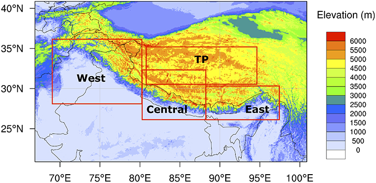
Figure 1. The High Mountain Asia (HMA) domain and the corresponding sub-regions with the terrain elevation as the background. Note that TP is the Tibetan Plateau.

2.2. Gridded Precipitation Datasets

Precipitation estimates from ten different products (i.e., APHRODITE, CHIRPS, IMD, CMORPH, TMPA, HAR, GDAS, ECMWF, ERA-Interim-Land, and MERRA2) are evaluated. Table 1 shows the general information of the datasets. APHRODITE (Asian Precipitation - Highly-Resolved Observational Data Integration Toward Evaluation) product is a daily gridded precipitation dataset for Asia that is generated from a dense network of daily rain-gauge data (Yasutomi et al., 2011; Yatagai et al., 2012). CHIRPS (Climate Hazards group Infrared Precipitation with Stations) dataset is a thermal infrared-based, quasi-global 0.05° precipitation (Funk et al., 2015). IMD (India Meteorological Department) precipitation data is a daily gridded rainfall product derived from a dense network of rain gage stations for the Indian mainland (Pai et al., 2014). In this study, 0.25° gridded rainfall dataset is used. CMORPH (CPC Morphing Technique) data is derived from several low orbit passive microwave observations (Joyce et al., 2004). TMPA (TRMM Multi-satellite Precipitation Analysis) is a merged multi-satellite precipitation product derived from the Tropical Rainfall Measuring Mission (TRMM) with a native spatial resolution of 0.25° (Huffman et al., 2007). In this study, we used the daily precipitation product called 3B42 (Version 7). As noted earlier, HAR is an atmospheric dataset generated primarily for the Tibetan Plateau using the Weather Research and Forecasting regional mesoscale model. The HAR precipitation estimates do not encompass any gauge-based precipitation measurements. GDAS (Global Data Assimilation System; Derber et al., 1991) is the global, operational atmospheric analysis system based on the operational Global Forecasting System developed at the Environmental Modeling Center of NOAA's National Centers for Environmental Prediction (NCEP). GDAS products were originally produced on a quadratic T170 gaussian grid (roughly 80 km) which subsequently have been upgraded to finer resolution data products over the years. The GDAS model grids have been upgraded to T254 (~60 km; since Oct 2002), T382 (~38 km; since Jun 2005), T574 (~27km; since Jul 2010) and T1534 (~13 km; since Jan 2015) for the years 2000–2015. The ECMWF data is obtained from the operational, global analysis products (Molteni et al., 1996) available on a T_L511 triangular truncation, linear reduced gaussian grid (0.25°) for four synoptic hours: 00, 06, 12, and 18 UTC. ERA-Interim/Land is a global reanalysis and is produced using the HTESSEL land surface model (Hydrology-Tiled ECMWF Scheme for Surface Exchanges over Land) with ERA-Interim forcing (Balsamo et al., 2015). Finally, MERRA2 (Modern-Era Retrospective Analysis for Research and Applications, version 2) is the latest atmospheric reanalysis from NASA Global Modeling and Assimilation Office and is produced with the Goddard Earth Observing System model version 5 (GEOS-5) Data Assimilation System (Gelaro et al., 2017). Note that GDAS, ECMWF, HAR, and MERRA2 are reanalysis products and include estimates of all surface meteorology variables whereas the other products contain estimates of precipitation only.

TABLE 1

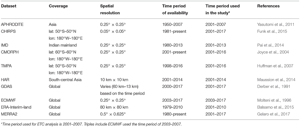
Table 1. Details of the precipitation datasets evaluated in this study.

2.3. Water Budget and Snow Evaluation Datasets

As reliable, independent reference datasets are sparse in this region, a thorough evaluation of each of the water budget components is difficult. Available remote sensing-based datasets of evapotranspiration (ET) and changes in terrestrial water storage (ΔTWS) and snow cover fraction (SCF) are used to provide evaluations of the LSM estimates as well as to provide indirect assessments of the driving meteorology.

Atmospheric Land Exchange Inverse model (ALEXI; Anderson et al., 2007) and the Global Land Evaporation Amsterdam Model (GLEAM; Martens et al., 2017) datasets are used to evaluate the modeled ET estimates. ET estimates in ALEXI are computed from surface temperature data derived from geostationary satellites within a two-source energy balance model. The ALEXI ET datasets available from 2003 at a 5 km resolution are used in this study. The GLEAM estimates are produced using a Priestley-Taylor approach driven by passive microwave sensor data, which does not involve aerodynamic and canopy resistance formulations, whereas all three LSMs employ a Penman Monteith type of formulation to compute ET. The GLEAM datasets from 2000 available at 0.25° spatial resolution are used here.

The Moderate Resolution Imaging Spectroradiometer (MODIS) daily SCF product from the Terra instrument (MOD10A1 version 6; Hall and Riggs, 2016) generated using the Normalized Difference Snow Index and a series of screens designed to alleviate errors and flag uncertain snow cover detections is used in this study. MOD10A1 data is available at 500 m spatial resolution from February 2000 to the present.

Terrestrial Water Storage (TWS), the total amount of water and ice mass on or within the Earth, as glaciers, permafrost, snow, soil moisture, surface water and groundwater, represents an integrated measure of the terrestrial water budget. Anomalies of TWS from the Gravity Recovery and Climate Experiment (GRACE; Tapley et al., 2004a) satellite are estimated after removing the effects of atmospheric and oceanic circulations and glacial isostatic adjustment. In this study, we employ three different GRACE products available on a monthly basis on 1° horizontal resolution grids from the University of Texas Center for Space Research, Jet Propulsion Laboratory, and German Research Centre for Geosciences. These products are based on the version RL05 spherical harmonics fields (Landerer and Swenson, 2012).

2.4. Land Surface Models and Configuration

To study terrestrial water budget components and their uncertainties, an ensemble of land surface model runs was conducted using a suite of LSMs and forcing inputs. Specifically, 12 different model runs were conducted using three different LSMs and four different forcing datasets. The Noah (version 3.3; Wang et al., 2010; Wei et al., 2013), Catchment (CLSM version Fortuna 2.5; Ducharne et al., 2000; Koster et al., 2000), and NoahMP (version 3.6; Niu et al., 2011; Yang et al., 2011) LSMs are forced with MERRA2, GDAS, and ECMWF meteorological boundary conditions. Note that we chose this subset of products for forcing the LSM runs as datasets such as APHRODITE, ERA-Interim-Land, HAR, and IMD have limited spatial or temporal coverage. Among the precipitation-only products (CHIRPS, CMORPH, TMPA), we choose CHIRPS data (with other near surface meteorology from ECMWF), since CHIRPS is found to have relatively low errors, high correlations and better consistency of trends in the precipitation evaluations discussed below (section 4.1).

The three LSMs represent a mix of models with significant differences in parameterizations and model physics, as documented in Kumar et al. (2017). The community Noah LSM is the land model currently used by NCEP and the United States Department of Defense to support their operational land analyses. Noah simulates the surface energy and water balance, land surface skin temperature, snowpack, soil temperature and moisture (both liquid and frozen) in multiple soil layers. The version of Noah used in this study includes several improvements and fixes to the snow physics and warm season processes (Wang et al., 2010). The NoahMP LSM is developed from the Noah LSM and incorporates extensive upgrades including dynamic vegetation phenology, a carbon budget and carbon-based photosynthesis, an explicit vegetation canopy layer, a multilayer snowpack representation and the addition of a groundwater module. The CLSM model represents the land component of the NASA GEOS-5 system. The subsurface water storage in CLSM is simulated using three prognostic bulk moisture variables that represent the deviations from the equilibrium soil moisture profile (Ducharne et al., 2000; Koster et al., 2000). A three-layer snow model simulates the snowpack evolution. The vertical moisture profile includes an implicit groundwater table located at the depth of equilibrium saturation. Note that none of these models configurations includes the treatment of glaciers and human management impacts of groundwater abstraction and irrigation.

The LSM simulations are conducted with a 15-min timestep for a 15-year time period (2003–2017) at 0.25 spatial resolution to generate daily output of water balance components. The initial conditions for the runs are generated by looping the LSMs from 2003 to 2017 twice, and then reinitializing the model in 2003. The LSMs are driven with meteorological datasets (MERRA2, GDAS, ECMWF, and CHIRPS) as described in section 4.1. The high-resolution elevation data from Shuttle Radar Topography Mission (Rodriguez et al., 2005) is used to derive the topography dataset of elevation, slope, and aspect. All model integrations use the modified International Geosphere Biosphere Programme MODIS 20-category landuse data (Friedl et al., 2002) and the soils data from the International Soil Reference and Information Centre (Hengl et al., 2014). The meteorological inputs (i.e., air temperature, humidity, surface pressure, wind, downward shortwave, and longwave radiation) are adjusted for the elevation differences through lapse-rate and slope-aspect correction methods (Kumar et al., 2013).

3. Methods

The meteorological inputs are evaluated through an intercomparison of the mean estimates and their seasonality. In addition, we employ indirect evaluation strategies such as the extended Triple Collocation (ETC; McColl et al., 2014) to assess the skill of the precipitation products. Note that the ETC does not require the availability of reference datasets. Thus, the ETC is effective to use for evaluation in this data poor region such as HMA, where reliable, spatially-representative reference measurements are not routinely available. We use the Mann-Kendall test (Mann, 1945; Kendall, 1975) to evaluate the statistical significance of the trends. To evaluate the uncertainties in the simulated water budget variables, reference measurements from remote sensing and reanalysis products are used. Here, commonly-used accuracy measures such as Root Mean Square Error (RMSE) and correlation coefficient (r) are utilized.

3.1. Extended Triple Collocation

Triple Collocation (TC; Stoffelen, 1998) is a method for the simultaneous estimation of the unknown error standard deviations (or RMSE) of three or more related datasets, without requiring knowledge of the "true" value. The method assumes a linear model (Equation 1) where the errors of the datasets being compared are orthogonal relative to the unknown truth and that the cross-error variance of the products are zero.

TC has been used in the evaluation of several earth system measurements such as soil moisture, ocean wind speed, leaf area index, and sea-ice thickness (Caires and Sterl, 2003; Fang et al., 2012; Roebeling et al., 2012; Zwieback et al., 2013; Gruber et al., 2016). The majority of the TC studies uses one dataset as a reference and applies rescaling procedures to ensure that the error orthogonality assumption is preserved and the system is solvable. Given three datasets (X₁, X₂, and X₃), we here rescale the other two precipitation products (X₂ and X₃) based on X₁ dataset, following Yilmaz and Crow (2014). Therefore, the RMSE estimated from TC can be assumed to be representative of the random error component of the total error.

McColl et al. (2014) introduced the ETC that can be used to estimate the RMSE and r between each of the triplets and the unknown truth. Note that ETC is mathematically equivalent to the original TC and provides an easier method for calculating the correlation coefficients. Alemohammad et al. (2015) introduced the multiplicative (logarithmic) error model to TC instead of the additive (linear) error model when applied to precipitation products across the United States. As the multiplicative error model is more appropriate for variables such as precipitation, this approach is used for evaluating the performance of precipitation products in section 4.1. Hence, a given precipitation estimate, X_i, can be written as:

$\begin{array}{ll}{X}_i=X_i^{{}^{\prime }}+{ϵ}_i={\alpha }_i+{\beta }_{i}t+{ϵ}_i& (1)\end{array}$

where X_i(i∈{1, 2, 3}) are collocated measurements that are linearly related to the (unknown) true value t, ϵ_i represents additive random errors, and α_i and β_i are offset and gain terms, respectively. Assuming that the errors are uncorrelated with each other (cov(ϵ_i, ϵ_j) = 0, i≠j) and with the (unknown) truth (cov(ϵ_i, t) = 0), the RMSE and r, can be estimated as:

$\begin{array}{ll}\begin{array}{cc}RMSE=\left[\begin{array}{l}\sqrt{Q_{11}-\frac{Q_{12}{Q}_{13}}{Q_{23}}}\hfill \\ \sqrt{Q_{22}-\frac{Q_{12}{Q}_{23}}{Q_{13}}}\hfill \\ \sqrt{Q_{33}-\frac{Q_{13}{Q}_{23}}{Q_{12}}}\hfill \end{array}\right]& r=\pm \left[\begin{array}{l}\sqrt{\frac{Q_{12}{Q}_{13}}{Q_{11}{Q}_{23}}}\hfill \\ sign(Q_{13}{Q}_{23})\sqrt{\frac{Q_{12}{Q}_{23}}{Q_{22}{Q}_{13}}}\hfill \\ sign(Q_{12}{Q}_{23})\sqrt{\frac{Q_{13}{Q}_{23}}{Q_{33}{Q}_{12}}}\hfill \end{array}\right]\end{array}& (2)\end{array}$

where Q_ij is the covariance of X_i and X_j. The signs, “+/-,” refer to positive linear correlation and negative correlation, respectively, but r will be practically expected to be positively corrected to the unobserved truth to avoid the sign ambiguity (McColl et al., 2014; Alemohammad et al., 2015).

3.2. Mann-Kendall Trend Test

The Mann-Kendall test is a non-parametric test for the monotonic trends of environmental data over time, such as climate data or hydrological data (Nguyen et al., 2018). The S statistics are calculated to determine increasing (or decreasing) pattern and their magnitude of the trend as follow:

$\begin{array}{ll}S={\Sigma }_{k=1}^{n-1}{\Sigma }_{j=k+1}^{n}sign(x_j-x_k)& (3)\end{array}$

where x is the time series variable. The subscript j and k are the observation time. sign(x_j − x_k) is equal to +1, 0, or -1, which means increasing, no, and decreasing trends, respectively. The S values are normalized to [-1, 1] for a better explanation. The null hypothesis H₀ assumes that there is no significant trend in the data at significant at a level of 5% (or 95% confidence level).

4. Results and Discussion

4.1. Precipitation Analysis

In this section, an intercomparison of the precipitation products is presented, in order to evaluate their suitability for land surface and hydrological model simulations. Figure 2 shows a comparison of the multi-annual mean precipitation over HMA (computed based on the available time period of each dataset shown in Table 1). The significant uncertainty in the precipitation estimates is evident in Figure 2. Generally, all datasets capture the spatial pattern of increased rainfall over the central and eastern regions compared to the west and the relatively dry regions of the Tibetan Plateau. A notable exception to this spatial pattern is ERA-Interim-Land, which shows significantly drier precipitation amounts compared to the other datasets. Though not as low as that of ERA-Interim-Land, the mean precipitation from MERRA2 is also low, particularly over the central and eastern regions. Among these datasets, the mean precipitation from ECMWF is the greatest, particularly over the eastern HMA. The pattern of larger precipitation magnitudes in these datasets is also seen over the western HMA, over parts of the Hindu Kush, and the Pamir mountains. Among the satellite-data based products (CHIRPS, CMORPH, TMPA), the magnitude of precipitation from CMORPH is lower and comparable to those from MERRA2 whereas the TMPA and CHIRPS estimates are larger and more consistent with the station-data based estimates from IMD and APHRODITE. Note that CHIRPS also includes information from the World Meteorological Organization Global Telecommunication System gauges, which are blended with infrared global Cold Cloud Duration estimates. The IMD and HAR datasets are not available over the entire domain of interest. The patterns of precipitation magnitudes from HAR show reasonable consistency with the gauge-based products, particularly over the eastern HMA. The boxplot in Figure 2 indicates that the model products HAR and GDAS have the largest spatial variability, whereas the gauge-based products (excluding IMD), show a more narrow range.

FIGURE 2

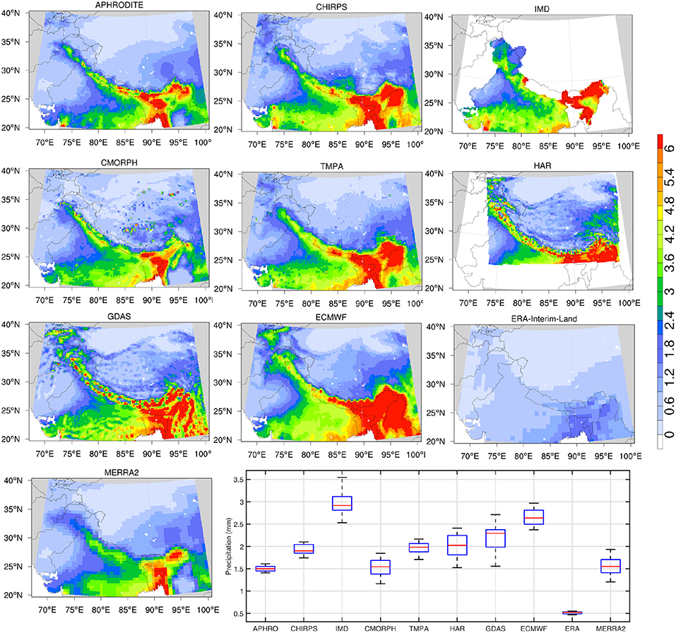
Figure 2. Spatial maps of multi-annual mean precipitation (mm) and their distribution from 10 precipitation datasets (Table 1). The box plot in the lower-right illustrates the median (red line), upper- and lower-quantiles (blue box) and the 25- and 75-th percentiles (black whiskers) of the multi-annual mean precipitation. Note that the IMD and HAR datasets are only available over part of the entire domain of interest.

To examine the differences among these datasets over the shallow and high terrain, a comparison of the domain-averaged mean precipitation stratified by elevation is shown in Figure 3. Similar to the patterns in Figure 2, ECMWF has higher mean precipitation than the other products at all elevations whereas ERA-Interim-Land, CMORPH, and MERRA2 are generally dry (Note that the spatial averages of IMD and HAR are influenced by their regional spatial coverage). Generally, there are larger differences in the precipitation estimates at lower elevations whereas the spread among the datasets reduces at higher elevation, likely due to the reduced influence of ground-based precipitation measurements. For example, precipitation magnitudes from APHRODITE at high elevations are low and comparable to that of MERRA2 and CMORPH. This pattern is consistent with the documented dry biases in APHRODITE over high terrain (Immerzeel et al., 2015). Similarly, the magnitude of precipitation from CHIRPS is larger than most products at low elevations. At higher elevations, however, the precipitation estimates from CHIRPS are lower than that of GDAS and ECMWF.

FIGURE 3

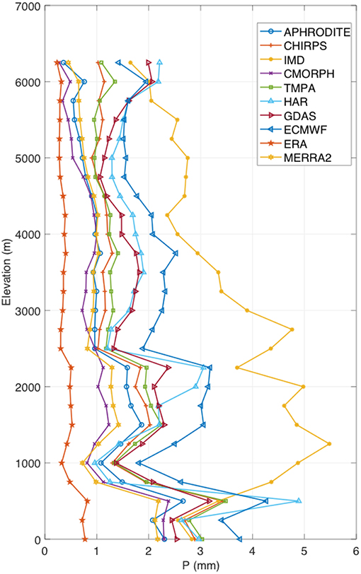
Figure 3. Comparison of the domain-averaged precipitation (P) stratified by elevation. Note that HAR and IMD datasets are limited in their spatial coverage.

The seasonal patterns of the spatial variability and magnitude of precipitation directly impact the snowpack evolution and melt processes. Since there are distinct precipitation regimes over HMA that influence the spatial patterns in winter and summer, the mean precipitation estimates stratified by the winter (December, January, February) and summer (June, July, August) time periods are shown in Figures 4, 5, respectively. The spatio-temporal patterns of the winter Westerlies are the primary determinant of snow evolution over these regions. Similar to Figure 2, the precipitation magnitudes are smallest in ERA-Interim-Land, followed by MERRA2 and CMORPH. The winter precipitation estimates are largest in the ECMWF, GDAS, and HAR products, whereas APHRODITE, CHIRPS, and IMD, which include information from gauges, span the intermediate range across these products. These patterns are repeated in the summer comparisons, where the precipitation regime shifts to the south and eastern regions (Figure 5). The magnitude of mean precipitation is lowest in ERA-Interim-Land and highest in ECMWF. The spatial pattern in MERRA2 over the eastern HMA during this time period is more consistent with APHRODITE, CHIRPS, and IMD, though the rainfall amounts are underestimated over the central HMA. These comparisons of mean precipitation are indicative of possible biases in these products. The seasonally stratified comparisons confirm that ECMWF and GDAS precipitation estimates are consistently high whereas MERRA2, ERA-Interim-Land, and the satellite-based products (TMPA and CMORPH) tend to be low. The gauge-informed products (particularly APHRODITE and CHIRPS) fall in the midrange in terms of the magnitude of precipitation in these comparisons.

FIGURE 4

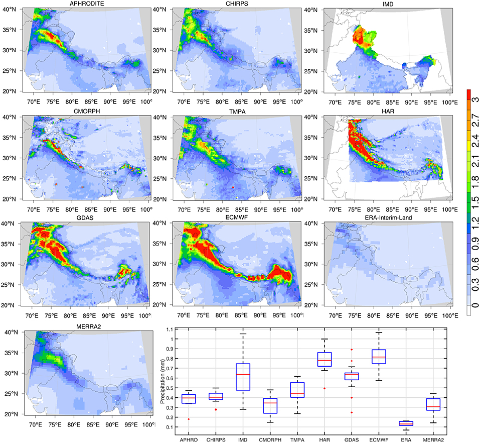
Figure 4. Same as Figure 2, but stratified for the peak winter months (December, January, February). The extreme data points/outliers are plotted individually using the “+” symbol.

FIGURE 5

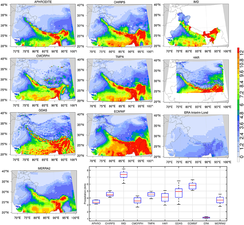
Figure 5. Same as Figure 2, but stratified for the summer months (June, July, August). The extreme data points/outliers are plotted individually using the “+” symbol.

Estimates of average RMSE and r² generated by the ETC analysis are shown in Figures 6, 7, respectively. These maps are generated by averaging the RMSE and r² values generated from each of the 120 possible triplets across the 10 precipitation products. As noted earlier, the RMSE estimates from ETC are representative of the random errors in these products. Figures 6, 7 indicate that MERRA2 products have the largest RMSEs and lowest r² values across different products. Comparatively, the station data-based products (APHRODITE, CHIRPS, and IMD) have lower errors and increased correlations (NOTE: the average error for IMD in the histogram is high because it only encompasses the Indian subcontinent). Generally, larger RMSEs are observed over the eastern HMA, likely because the mean precipitation is higher over the eastern region due to the influence of the monsoon regime. Conversely, low RMSEs are observed over the Tibetan Plateau from most products, as precipitation magnitudes are typically small in that region. Among the model-based precipitation products, ECMWF performs well with low RMSE and high r² values. It is also notable that in ECMWF, r² estimates are consistently high across the entire domain and the spatial variability of r² is generally low, particularly compared to the spatial patterns of r² in other datasets. The satellite-based products (CMORPH and TMPA) have low correlations over the Tibetan Plateau and high elevation areas whereas the correlations are higher in the southern parts of the domain. Note that the products that include in-situ measurements (APHRODITE, CHIRPS, IMD) may share information from the same station locations. In such cases, the assumption of uncorrelated errors in the triplets may be violated. In the ETC evaluations shown in Figures 6, 7, however, the influence of correlated errors is ignored as the spatial density of the stations is small and time span of the individual station data products is different.

FIGURE 6

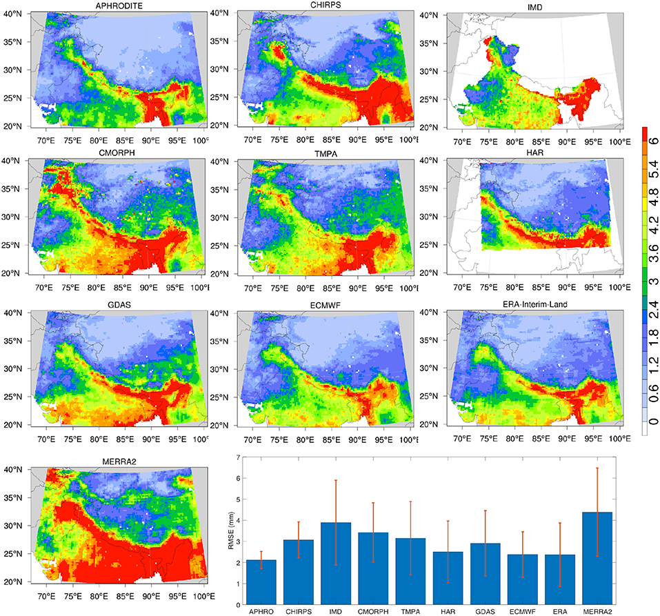
Figure 6. RMSE of precipitation (mm) estimated using the ETC method. The value at each grid point represents the mean RMSE across 120 possible triplets among the 10 precipitation products. The error bars represent the mean standard deviation across the 120 triplets.

FIGURE 7

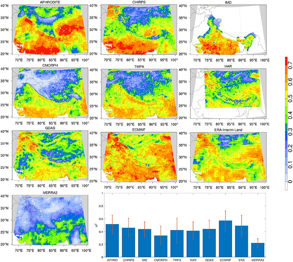
Figure 7. Same as Figure 6, but for r².

Figure 8 shows the domain-averaged mean annual precipitation from these datasets along with estimates of their temporal trends for the four sub-regions of HMA (Figure 1). Note that for some datasets (IMD and HAR), the spatial averages are influenced by their limited spatial coverage.

FIGURE 8

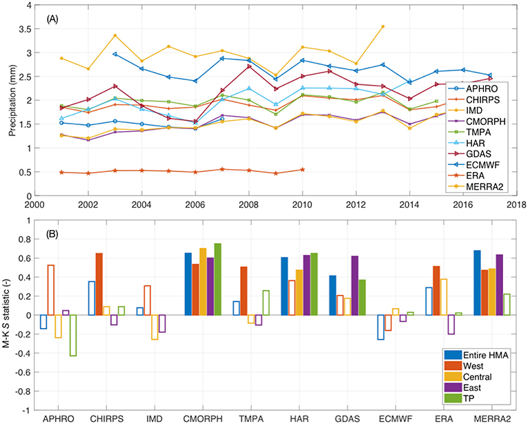
Figure 8. Time series of domain-averaged mean annual precipitation (A), and estimates of the Mann Kendall S-statistic (B) for the entire HMA and four sub-regions (Figure 1). The statistically significant trends are shown with filled boxes.

CMORPH, GDAS, HAR, and MERRA2 show an increasing trend of precipitation over all of HMA, whereas the other datasets do not indicate a statistically significant increasing or decreasing trend. There are more significant trends in the regional evaluations. Over the western HMA, most products indicate an increasing precipitation trend, consistent with the findings of Nguyen et al. (2018). None of the products show a statistically significant decreasing trend in precipitation over the central and eastern regions as suggested in Nguyen et al. (2018) and Rodell et al. (2018). In fact, CMORPH, HAR, and MERRA2 show the opposite trend, indicating a statistically significant increasing trend in precipitation. Finally, over the Tibetan Plateau, most products except CMORPH, GDAS, and HAR indicate no significant trends in precipitation. Note that over the Tibetan Plateau, Rodell et al. (2018) found an increasing trend in precipitation whereas Nguyen et al. (2018) indicates that there is no statistically significant trend in precipitation. It should also be stressed that the time periods (i.e., 17-year analysis) used in our computations are generally short, due to the availability of datasets, and the choice of a common time period of evaluation. The shortness of the time period of evaluation is a likely contributing factor in the determination of these trends.

It should be emphasized that the sparse and uneven in-situ coverage in these precipitation products is a significant factor in the quality of these products, as documented in prior studies (Ghatak et al., 2018). Generally, it is acknowledged that precipitation is underestimated in these products, particularly over high elevations (Immerzeel et al., 2015). Most weather stations are located on the valley floors (at lower elevation) and not on mountain slopes, which means that statistically-averaged gauge data may not properly represent the heterogeneity of rainfall in complex terrain over these regions (Bharti and Singh, 2015; Song et al., 2016). The retrieval algorithms for satellite-based products can suffer from high frequency microwave scattering associated with persistent snow cover and falling snow in high mountainous regions, which contributes to the uncertainty in these products (Yong et al., 2015; Song et al., 2016). The accuracy and the trends in the modeled precipitation products are also influenced by the remote sensing inputs. For example, it is documented (Bosilovich et al., 2017) that the introduction of the Atmospheric Infrared Sounder radiances in 2002 leads to an increase in precipitation over the land areas and a decrease over the oceans. Bosilovich et al. (2017) also note that the introduction of data from new instruments is a significant factor in the changes of water cycle components in these reanalysis products.

4.2. Near Surface Air Temperature Analysis

An intercomparison of near surface air temperature (T_air) estimates from three model analysis products (ECMWF, GDAS, and MERRA2) is presented in this section. A time series of domain-averaged annual mean T_air estimates from 2000-onward is shown in Figure 9, which demonstrates the significant differences in the mean and the trends in these products. The MERRA2 estimates are generally warmer and devoid of any climatological trends, whereas both ECMWF and GDAS estimates show a statistically significant warming trend, with generally cooler T_air than that of MERRA2. When stratified regionally, GDAS shows a warming trend over all four regions, whereas ECMWF shows warming trends in the western and central regions only. MERRA2 does not have a statistically significant trend in the western and central regions, whereas it shows an increasing trend in T_air over the Tibetan Plateau and eastern regions. Previous studies using in-situ measurements and GCM outputs also find the climatological warming trends in the eastern (Ren et al., 2017), central (Shrestha et al., 1999), and the Tibetan Plateau (Immerzeel, 2008) regions.

FIGURE 9

Figure 9. Time series of domain-averaged mean annual near surface air temperature (A), and estimates of the Mann Kendall S-statistic (B) for the entire HMA and four sub-regions (Figure 1). The statistically significant trends are shown with filled boxes.

The time series of annual mean T_air shown in Figure 9 indicates that MERRA2 is consistently warmer than GDAS and ECMWF. The examination of the mean seasonal cycle of T_air also confirms that the pattern of warmer T_air in MERRA2 is persistent throughout the season (not shown). In particular, over most of the eastern HMA, climatological mean T_air from MERRA2 is observed to be above freezing. GDAS estimates are comparable to MERRA2 during the summer time period and are coldest (among the three products) during the winter time periods. The evaluation of T_air presented in this section indicates that the lack of a warming trend, consistently warmer estimates and regional deficiencies in the seasonality of MERRA2 estimates poses significant challenges for realistic snow and hydrological model simulations.

4.3. Uncertainties in the Water Cycle Components

In this section, we examine the uncertainty in the terrestrial water balance estimates from the LSM ensemble. The terrestrial water budget is represented by Equation (4), representing the partitioning of total precipitation (P) into ET, runoff (R), and ΔTWS. Note that R is the gridded runoff (consisting of surface runoff and baseflow) estimated by the LSM and not the routed streamflow. The ΔTWS are contributed by the changes in soil moisture, snow ice mass, canopy water, surface water, and ground water storages.

$\begin{array}{ll}P=ET+R+\Delta TWS& (4)\end{array}$

We first examine if the spread in P, ET, and R is driven by the differences in the LSM formulations or the driving meteorology. Figure 10 shows the distribution of mean annual averages of P, ET, and R, grouped by LSMs and the forcing datasets. Overall, it can be noted that there are smaller differences in the water budget terms across the LSMs when driven with a common forcing whereas larger differences in P, ET, and R are seen across the modeled estimates with different forcing datasets. This suggests that the uncertainty in the driving meteorology is the dominant factor in the terrestrial water budget estimates. Generally, the spread in the ET estimates (when grouped by the LSM or the forcing) is generally small compared to that seen with R. It can be noted that, when stratified by the forcing dataset, the range of ET and R estimates essentially mirrors that of the precipitation input. Indeed, similar to the precipitation inputs, the magnitude of ET and R is higher during the summer season over eastern HMA (not shown). During the melt season, due to the contribution of snow and ice melt to R, the spatial patterns of R shift from northwest to southeast. The high and low estimates of ET and R are obtained from LSM runs that employ ECMWF and MERRA2, respectively. These results further confirm the significant influence of precipitation in the LSM-based water budget estimates.

FIGURE 10

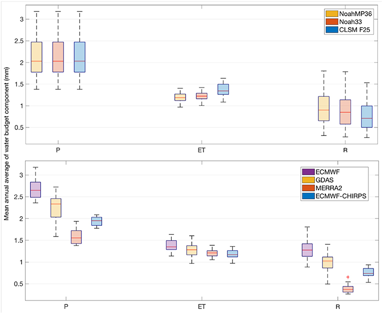
Figure 10. Distribution of the mean annual averages of precipitation (P), evapotranspiration (ET) and total runoff (R), grouped by the LSMs (top panel) and forcing datasets (bottom panel). The units are mm.

Across the 12 member LSM ensemble used in this study, we estimate the mean annual fluxes and their uncertainty (expressed as one standard deviation) over HMA in P, ET, and R to be 2.11 ± 0.45, 1.26 ± 0.11, and 0.85 ± 0.36 mm per day, respectively. Similar estimates are seen in global water budget estimation studies. For example, using a large suite of modeled and remote sensing based products, Rodell et al. (2015) document that the annual mean fluxes and their uncertainty at the global scale to be 2.16 ± 0.12, 1.33 ± 0.13, and 0.92 ± 0.13 mm per day, for P, ET, and R, respectively. The estimates over Eurasia are similar, with annual mean fluxes of 1.99 ± 0.12, 1.15 ± 0.18, and 0.94 ± 0.12 mm per day in P, ET, and R, respectively.

The mean annual estimates from our model ensemble are comparable to these global/continental estimates, while the uncertainty estimates, particularly for P and R, are significantly higher than the corresponding global estimates, which is an additional confirmation of the challenges in the accurate characterization of these terrestrial fluxes over HMA. These uncertainties estimates are also quite close to those found by Munier and Aires (2018).

Figure 11 shows the distribution of the domain-averaged RMSE from each model run as well as maps of the ensemble mean RMSE across the 12 ensemble members. Though independent, ALEXI and GLEAM are also modeled products, with their own biases in the ET estimates, which are apparent in the comparisons shown in Figure 11. In the ALEXI comparisons, estimates from Noah33 and NoahMP forced with ECMWF produce the lowest RMSE, whereas NoahMP forced with ECMWF and CHIRPS produces the best agreement compared to GLEAM. The examination of the mean seasonal cycles of the model runs and these reference products indicates that the ET estimates from ALEXI are generally higher compared to the LSM ensemble. Note that similar findings about the possible positive biases in ALEXI are also described in Ghatak et al. (2018). That means a better match of a model run with ALEXI may be indicative of a high bias in the modeled estimates. GLEAM, on the other hand, shows better consistency with the model ensemble, though the ET magnitudes are lower in the late summer, fall, and winter months. In the GLEAM comparisons, runs forced with ECMWF and CHIRPS produce the best agreements in ET for each model. In the spatial comparisons, larger disagreements are seen over the western regions and parts of the eastern domain. The RMSE spatial patterns in the GLEAM comparison essentially mirror the summer precipitation means (Figure 5) with the disagreements more prominent over the eastern parts of the domain. Figure 11 also indicates that the disagreements between LSMs and ALEXI are more prominent over the lower Indus and lower Brahmaputra basins. These basins are known to have significant agricultural irrigation systems (http://pakirsa.gov.pk), the impacts of which are not captured in the LSM runs. It is possible that the large RMSE values over these areas are a result of the reference datasets capturing the impacts of such processes. ALEXI, in particular, has been demonstrated to represent the impacts of management related sources and sinks over the continental United States (Hain et al., 2015).

FIGURE 11

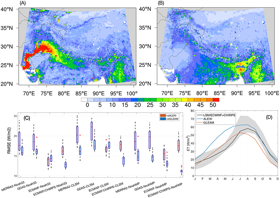
Figure 11. Maps of ensemble mean RMSE (W/m²) of ET across the 12 ensemble members compared against ALEXI (A) and GLEAM (B), distribution of the domain-averaged RMSE from each of the 12 LSM runs (C) and the mean seasonal cycle of ET (D). The gray shading in (D) represents the spread in ET across the LSMs.

As reliable, multi-year ground observations of R are not easily available over this domain, an independent assessment of the quality of R estimates beyond the comparisons shown in Figure 10 is not conducted in this study. Instead, we focus on the assessment of the simulated TWS and snow conditions. Note that a direct evaluation of the snow mass is difficult due to the lack of reliable ground measurements with good spatial coverage. In addition, remote sensing retrievals of SWE and snow depth from passive microwave instruments retrievals are known to have large uncertainties in mountainous terrain such as HMA (Dong et al., 2005; Markus et al., 2006; Tedesco et al., 2010). Therefore, the evaluation of snow conditions is performed by comparing the simulated SCF estimates against the observations from the MODIS instrument, which provides an assessment of the snow covered extent, but not the snow mass.

Figure 12 shows a comparison of mean SCF from MOD10A1 and the modeled SCF averaged across the LSMs for each forcing data. The influence of the precipitation and temperature differences in the driving meteorology can be observed in these comparisons. The large magnitude of precipitation in the ECMWF and GDAS data leads to large snow evolution and broader spatial coverage of snow. This is evidenced in both the spatial maps and in the comparison of the mean SCF stratified by elevation. The snow coverage in the MERRA2 based runs, on the other hand, is generally low, possibly due to the underestimation of precipitation and warmer air temperature. The CHIRPS-based runs provide a better match with the MOD10A1 data, particularly over the western and central domains and over the mid-elevation ranges (~ 2,000–5,000 m). In the southeast part of the domain, the CHIRPS-based runs underestimate snow coverage, due to possible precipitation underestimation. The accuracy of simulating snow cover is evaluated using the probability of detection (POD) and false alarm ratio (FAR) compared to MOD10A1. Overall, the LSM ensemble has an average POD of 72% and FAR of 36%. Most prominent POD and FAR values are over the shallow snow covered areas over the Tibetan Plateau and eastern HMA. Despite these discrepancies over eastern HMA, the ECMWF + CHIRPS-based runs provide the best estimate of the snow coverage, with a domain average POD of 81% albeit with a slightly higher FAR of 51%.

FIGURE 12

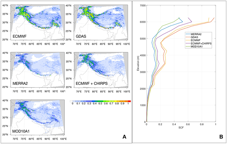
Figure 12. Comparison of mean SCF estimates (unitless) from MOD10A1 and the model runs. (A) Shows the spatial maps of mean SCF whereas (B) shows the domain-averaged SCF stratified by elevation. The modeled estimates are averaged across the three LSMs for each forcing data.

Figure 13 shows the time series of the spread of TWS anomalies from GRACE and the model runs during 2003–2018. Over the entire HMA, the model runs provide a reasonable match to GRACE, though the slight declining trend in TWS is not represented well in the model runs. Larger differences between the modeled estimates and GRACE are observed in the regional comparisons. As noted in Rodell et al. (2018), significant declining trends in GRACE are observed over the western and central regions. The negative trends in TWS anomalies are comparatively smaller over the eastern HMA. The model runs do not represent these temporal trends well, as none of the input precipitation forcing data used in the model ensemble (ECMWF, GDAS, MERRA2, and CHIRPS) has a statistically significant declining trend over this region. Since MERRA2 has an increasing trend in precipitation, the MERRA2 forced run shows an increasing trend in TWS. The domain-averaged anomaly RMSE and R of the LSM ensemble are 67 mm and 0.31, respectively. The dominant errors come from glacial areas and downstream basins of the western and central HMA. Overall, average anomaly RMSE and r of the ECMWF+CHIRPS runs are 59 mm and 0.36, respectively, providing the best match to the GRACE observations. Note that the TWS anomalies from the ECMWF+CHIRPS runs are also shown as a separate time series in Figure 13.

FIGURE 13

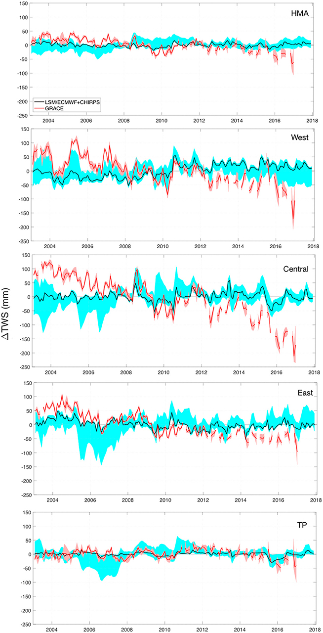
Figure 13. The time series of the anomalies in TWS (mm) from GRACE and the model runs during 2003–2018. The red and cyan shadings represent the spread in TWS anomalies across the GRACE products and LSMs, respectively. The average TWS anomaly estimates from models driven by the ECMWF +CHIRPS forcing are shown in black.

Note that relating the surface mass changes to the GRACE signal can be hard in this region with tectonically active mountain ranges, substantial groundwater pumping for farm irrigation, and melting of snow and glaciers (Moiwo et al., 2011; Immerzeel and Bierkens, 2012). Rodell et al. (2018) identified groundwater depletion as the primary cause of the declining trends in TWS over the western HMA whereas water depletion and precipitation decline was the key reason for the decline in TWS over the central and eastern HMA. Studies such as Moiwo et al. (2011) and Yi and Sun (2014) also quantify that the influence of the mass changes from glacier melt is comparable to that from underground water depletion over HMA. As the LSM simulations used in this study exclude glaciers and do not include representations of human management such as groundwater abstractions, they can only be expected to simulate the impacts of natural variability in meteorology. The mismatches between the model estimates and GRACE TWS in Figure 13, therefore, can be used to find potential sources of TWS variability and limitations of precipitation inputs. For example, over the Tibetan Plateau, the model (particularly the ECMWF+CHIRPS based simulation) and GRACE estimates are comparable, indicative of the reasonable quality of the input meteorology. Comparatively, the larger mismatches over the West and Central regions can be attributed to the lack of handling of the glacier melt and groundwater abstraction impacts in the model.

5. Summary and Conclusions

Despite the importance of HMA as a critically important area of freshwater storage and water availability, significant uncertainty in the characterization of terrestrial water budget components exists due to the lack of reliable and spatially-distributed ground measurements as well as limitations in the modeling and remote sensing estimates. This study presents an evaluation of the key terrestrial water budget variables over HMA using available measurements and both direct and indirect evaluation methods. An ensemble of uncoupled land surface model simulations forced with prescribed meteorology is used to develop estimates of terrestrial water budget components.

As precipitation is one of the most important inputs for LSM simulations, an evaluation of the quality of a suite of 10 precipitation datasets is conducted first. The spatial patterns of precipitation seasonality, where the winter precipitation is dominated by the westerly and southwesterly flows with the summer precipitation influenced primarily by the South Asia monsoon, are captured reasonably well in these products. However, significant differences in the mean estimates are observed across these products. Within the suite of products being compared, the precipitation magnitudes from ERA-Interim-Land and MERRA2 are generally lower whereas that from GDAS and ECMWF are higher. The station data and remote sensing based products generally encapsulate an intermediate range of precipitation variability in the comparisons.

An indirect evaluation method called ETC that does not require the availability of a reference dataset is used to assess the RMSE and correlation of these precipitation data products. The ETC evaluation indicates poor performance of MERRA2 with large RMSE and low r² values. The products such as APHRODITE, CHIRPS, and IMD that employ gauge information had stronger agreement across the ETC comparisons. Among the modeled estimates, the ECMWF dataset is found to have good skill with low RMSE and high correlations. Spatially, larger errors are observed over the eastern HMA, where the magnitude of the precipitation is higher than the western and central domains due to the influence of the South Asia monsoon. The examination of the temporal trends in the precipitation datasets also demonstrates significant differences across these products. CMORPH, GDAS, HAR, and MERRA2 show an increasing trend of precipitation over HMA, whereas the other datasets do not show a statistically significant increasing or decreasing trend. The increasing precipitation trends in these products, particularly over the central and eastern regions, are inconsistent with the reported declining trends in prior studies.

A comparison of the T_air from ECMWF, GDAS, and MERRA2 indicates that MERRA2 estimates are generally warmer. Consistent with the prior studies, ECMWF and GDAS T_air estimates indicate a warming trend whereas MERRA2 estimates do not show a significant warming or cooling trend. These inconsistencies (in precipitation and air temperature) have significant influence on the LSM simulations, particularly in the characterization of the magnitude of snowpack evolution over HMA.

Using a subset (ECMWF, GDAS, MERRA2, and CHIRPS) of the 10 precipitation products, 12 model runs are conducted using three different land surface models. This model ensemble is used to generate assessments of the uncertainty in the terrestrial water budget components. Comparison of the distribution of the mean annual averages of P, ET, and R stratified by the driving meteorology and LSMs indicates that the uncertainty in the driving meteorology is the dominant factor in the uncertainty in these estimates over HMA. Further, there is larger uncertainty in the R estimates compared to the spread in the ET estimates within the ensemble. The annual mean estimates of water budget partition from this model ensemble are found to be comparable to reported global/continental estimates in prior studies, whereas the uncertainty/spread of P, ET, and R is significantly larger than the corresponding estimates from global studies.

The modeled ET estimates are compared against the thermal infrared based ALEXI and passive microwave based GLEAM estimates. Generally, the biases in the input precipitation datasets (particularly over the summer months) are reflected in the quality of the ET estimates, with the model runs forced by ECMWF + CHIRPS producing the best match with the GLEAM estimates. The modeled SCF estimates are strongly influenced by the input precipitation and air temperature. The ECMWF and GDAS based runs produce large snow evolution whereas MERRA2 runs underestimate the magnitude and extent of snow. Overall, the ECMWF+CHIRPS based run provides the best match to the MOD10A1 estimates, particularly over the western and central HMA. Though the ECMWF+CHIRPS based runs underestimate the snow evolution in the northeastern parts of HMA, such disagreements are mostly limited to areas with shallow snow. When compared at the domain-wide scale, the simulated TWS anomalies show reasonable agreements with those from the GRACE mission. In regional comparions the model simulations fail to simulate the declining trends in TWS observed in GRACE. The lack of a statistically significant declining trend in precipitation is the cause of this deficiency in some parts of the domain (over the Central HMA). Over HMA, the GRACE signal also encompasses the impacts of groundwater pumping, tectonic activity, and glacier melt, which are not well represented in the LSM simulations. The discrepancies between GRACE and the LSM estimates (particularly over the Western and Central HMA) are likely due to these missing processes in the LSM simulations.

Overall, this study points to the significant need for improving the meteorological boundary conditions toward reducing the uncertainty in the terrestrial budget estimates. The results presented in this article demonstrate that some of the widely used global reanalysis products have significant uncertainties in their surface meteorological fields in such a mountainous region and these uncertainties are accompanied by a failure to capture trends and inter-annual variability relevant to water resource monitoring and projection applications. While direct measurements of variables such as precipitation are difficult over this complex terrain, the study demonstrates the utility of indirect evaluation methods for developing attributions of uncertainty. For example, the use of remotely sensed SCF measurements to assess precipitation products is particularly useful in mid-elevation zones where the biases in input precipitation are expected to lead to biases in simulated SCF. The challenge in evaluating remotely sensed ET products remains a critical gap, as there is significant uncertainty in the absolute values generated by products such as ALEXI and GLEAM. These products, however, are still useful for evaluating the spatial and temporal variability of the simulated ET products (Anderson et al., 2007; Martens et al., 2017). Similarly, the lack of reliable, spatially distributed measurements of SWE, particularly at higher elevations, is another critical terrestrial water budget observational gap. As evidenced in this study, despite its importance as a major water budget component, reliable measurements of R are lacking in this region due to the limitations of the stream gauge network and inadequate data sharing. Measurements from the upcoming Surface Water Ocean Topography (Biancamaria et al., 2016) mission are expected to help toward mitigating this observational gap. The current study provides a benchmark for evaluating further improvements in water budget estimation through the incorporation of such future measurements.

Author Contributions

YY and SK performed background research, designed the experiments, and led the analysis with the help of BF, BZ, YK, YQ, SR, VM, PH, DK, AR, and AA. DM and JJ helped to analyze and interpret the model results. YY and SK wrote the majority of the manuscript. SB and AM assisted in assembling the IMD precipitation dataset. All authors contributed toward the interpretation of the results.

Funding

Funding for this work was provided by NASA's High Mountain Asia research program.

Conflict of Interest Statement

The authors declare that the research was conducted in the absence of any commercial or financial relationships that could be construed as a potential conflict of interest.

Acknowledgments

We acknowledge the assistance from the NASA Center for Climate Simulation for conducting the model simulations and analyses.

References

Alemohammad, S. H., McColl, K. A., Konings, A. G., Entekhabi, D., and Stoffelen, A. (2015). Characterization of precipitation product errors across the United States using multiplicative triple collocation. Hydrol. Earth Syst. Sci. 19, 3489–3503. doi: 10.5194/hess-19-3489-2015

CrossRef Full Text | Google Scholar

Andermann, C., Bonnet, S., and Gloaguen, R. (2011). Evaluation of precipitation data sets along the Himalayan front. Geochem. Geophys. Geosyst. 12:Q07023. doi: 10.1029/2011GC003513

CrossRef Full Text | Google Scholar

Anderson, M. C., Norman, J. M., Mecikalski, J. R., Otkin, J. A., and Kustas, W. P. (2007). A climatological study of evapotranspiration and moisture stress across the continental United States based on thermal remote sensing: 1. Model formulation. J. Geophys. Res. 112:D10117. doi: 10.1029/2006JD007506

CrossRef Full Text | Google Scholar

Balsamo, G., Albergel, C., Beljaars, A., Boussetta, S., Brun, E., Cloke, H., et al. (2015). ERA-Interim/Land: a global land surface reanalysis data set. Hydrol. Earth Syst. Sci. 19, 389–407. doi: 10.5194/hess-19-389-2015

CrossRef Full Text | Google Scholar

Barlow, M., Wheeler, M., Lyon, B., and Cullen, H. (2005). Modulation of daily precipitation over Southwest Asia by the Madden–Julian oscillation. Month. Weather Rev. 133, 3579–3594. doi: 10.1175/MWR3026.1

CrossRef Full Text | Google Scholar

Bharti, V., and Singh, C. (2015). Evaluation of error in TRMM 3B42V7 precipitation estimates over the Himalayan region. J. Geophys. Res. 120, 12458–12473. doi: 10.1002/2015JD023779

CrossRef Full Text | Google Scholar

Biancamaria, S., Lettenmaier, D. P., and Pavelsky, T. M. (2016). The SWOT mission and its capabilities for land hydrology. Surv. Geophys. 37, 307–337. doi: 10.1007/s10712-015-9346-y

CrossRef Full Text | Google Scholar

Bookhagen, B., and Burbank, D. W. (2010). Toward a complete Himalayan hydrological budget: spatiotemporal distribution of snowmelt and rainfall and their impact on river discharge. J. Geophys. Res. 115:F03019. doi: 10.1029/2009JF001426

CrossRef Full Text | Google Scholar

Bosilovich, M. G., Robertson, F. R., Takacs, L., Molod, A., and Mocko, D. (2017). Atmospheric water balance and variability in the MERRA-2 reanalysis. J. Clim. 30, 1177–1196. doi: 10.1175/JCLI-D-16-0338.1

CrossRef Full Text | Google Scholar

Caires, S., and Sterl, A. (2003). Validation of ocean wind and wave data using triple collocation. J. Geophys. Res. 108:3098. doi: 10.1029/2002JC001491

CrossRef Full Text | Google Scholar

Derber, J. C., Parrish, D. F., and Lord, S. J. (1991). The new global operational analysis system at the national meteorological center. Weather Forecast. 6, 538–547.

Google Scholar

Dong, J., Walker, J., and Houser, P. (2005). Factors affecting remotely sensed snow water equivalent uncertainty. Remote Sens. Environ. 97, 68–82. doi: 10.1016/j.rse.2005.04.010

CrossRef Full Text | Google Scholar

Ducharne, A., Koster, R., Suarez, M., Stieglitz, M., and Kumar, P. (2000). A catchment-based approach to modeling land surface processes in a general circulation model, 2, Parameter estimation and model demonstration. J. Geophys. Res. 105, 24823–24838. doi: 10.1029/2000JD900328

CrossRef Full Text | Google Scholar

Fang, H., Wei, S., Jiang, C., and Scipal, K. (2012). Theoretical uncertainty analysis of global MODIS, CYCLOPES, and GLOBCARBON LAI products using a triple collocation method. Remote Sens. Environ. 124, 610–621. doi: 10.1016/j.rse.2012.06.013

CrossRef Full Text | Google Scholar

Foster, J., Sun, C., Walker, J., Kelly, R., Chang, A., Dong, J., et al. (2005). Quantify the uncertainty in passive microwave snow water equivalent observations. Remote Sens. Environ. 94, 187–203. doi: 10.1016/j.rse.2004.09.012

CrossRef Full Text | Google Scholar

Friedl, M., McIver, D., Hodges, J., Zhang, X., Muchoney, D., Strahler, A., et al. (2002). Global land cover mapping from MODIS: algorithms and early results. Remote Sens. Environ. 83, 287–302. doi: 10.1016/S0034-4257(02)00078-0

CrossRef Full Text | Google Scholar

Funk, C., Peterson, P., Landsfeld, M., Pedreros, D., Verdin, J., Shukla, S., et al. (2015). The climate hazards infrared precipitation with stations - a new environmental record for monitoring extremes. Sci. Data 2:150066. doi: 10.1038/sdata.2015.66

PubMed Abstract | CrossRef Full Text | Google Scholar

Galewsky, J. (2009). Rain shadow development during the growth of mountain ranges: an atmospheric dynamics perspective. J. Geophys. Res. Earth Surf. 114:F01018. doi: 10.1029/2008JF001085

CrossRef Full Text | Google Scholar

Gelaro, R., McCarty, W., Suárez, M. J., Todling, R., Molod, A., Takacs, L., et al. (2017). The modern-era retrospective analysis for research and applications, version 2 (MERRA-2). J. Clim. 30, 5419–5454. doi: 10.1175/JCLI-D-16-0758.1

CrossRef Full Text | Google Scholar

Ghatak, D., Zaitchik, B., Kumar, S., Matin, M. A., Bajracharya, B., Hain, C., et al. (2018). Influence of precipitation forcing uncertainty on hydrological simulations with the NASA South Asia land data assimilation system. Hydrology 5:57. doi: 10.3390/hydrology5040057

CrossRef Full Text | Google Scholar

Gruber, A., Su, C.-H., Zwieback, S., Crow, W., Dorigo, W., and Wagner, W. (2016). Recent advances in (soil moisture) triple collocation analysis. Int. J. Appl. Earth Observ. Geoinform. 45, 200–211. doi: 10.1016/j.jag.2015.09.002

CrossRef Full Text | Google Scholar

Guo, Z., Dirmeyer, P. A., Hu, Z.-Z., Gao, X., and Zhao, M. (2006). Evaluation of the second global soil wetness project soil moisture simulations: 2. Sensitivity to external meteorological forcing. J. Geophys. Res. 111:D22S02. doi: 10.1029/2006JD007845

CrossRef Full Text | Google Scholar

Hain, C. R., Crow, W. T., Anderson, M. C., and Yilmaz, M. T. (2015). Diagnosing neglected soil moisture source–sink processes via a thermal infrared–based two-source energy balance model. J. Hydrometeorol. 16, 1070–1086. doi: 10.1175/JHM-D-14-0017.1

CrossRef Full Text | Google Scholar

Hall, D., and Riggs, G. (2016). MODIS/Terra Snow Cover Daily L3 Global 500m Grid, Version 6. Technical report, National Snow and Ice Data Center Distributed Active Archive Center.

Google Scholar

Hall, D. K., Riggs, G. A., and Salomonson, V. V. (1995). Development of methods for mapping global snow cover using moderate resolution imaging spectroradiometer data. Remote Sens. Environ. 54, 127–140. doi: 10.1016/0034-4257(95)00137-P

CrossRef Full Text | Google Scholar

Hengl, T., de Jesus, J., MacMillan, R., Batjes, N., Heuvelink, G., Ribeiro, E., et al. (2014). SoilGrids1km - global soil information based on automated mapping. PLoS ONE 9:e105992. doi: 10.1371/journal.pone.0105992

PubMed Abstract | CrossRef Full Text | Google Scholar

Hewitt, K. (2011). Glacier change, concentration, and elevation effects in the Karakoram Himalaya, Upper Indus basin. Moutain Res. Dev. 31, 188–200. doi: 10.1659/MRD-JOURNAL-D-11-00020.1

CrossRef Full Text | Google Scholar

Huffman, G. J., Bolvin, D. T., Nelkin, E. J., Wolff, D. B., Adler, R. F., Gu, G., et al. (2007). The TRMM multisatellite precipitation analysis (TMPA): quasi-global, multiyear, combined-sensor precipitation estimates at fine scales. J. Hydrometeorol. 8, 38–55. doi: 10.1175/JHM560.1

CrossRef Full Text | Google Scholar

Immerzeel, W. (2008). Historical trends and future predictions of climate variability in the Brahmaputra basin. Int. J. Climatol. 28, 243–254. doi: 10.1002/joc.1528

CrossRef Full Text | Google Scholar

Immerzeel, W., and Bierkens, M. (2012). Asia's water balance. Nat. Geosci. 12, 841–842. doi: 10.1038/ngeo1643

CrossRef Full Text | Google Scholar

Immerzeel, W., Droogers, P., de Jong, S., and Bierkens, M. (2009). Large-scale monitoring of snow cover and runoff simulation in Himalayan river basins using remote sensing. Remote Sens. Environ. 113, 40–49. doi: 10.1016/j.rse.2008.08.010

CrossRef Full Text | Google Scholar

Immerzeel, W. W., van Beek, L. P. H., and Bierkens, M. F. P. (2010). Climate change will affect the Asian water towers. Science 328, 1382–1385. doi: 10.1126/science.1183188

PubMed Abstract | CrossRef Full Text | Google Scholar

Immerzeel, W. W., Wanders, N., Lutz, A. F., Shea, J. M., and Bierkens, M. F. P. (2015). Reconciling high-altitude precipitation in the upper Indus basin with glacier mass balances and runoff. Hydrol. Earth Syst. Sci. 19, 4673–4687. doi: 10.5194/hess-19-4673-2015

CrossRef Full Text | Google Scholar

Joyce, R. J., Janowiak, J. E., Arkin, P. A., and Xie, P. (2004). CMORPH: a method that produces global precipitation estimates from passive microwave and infrared data at high spatial and temporal resolution. J. Hydrometeorol. 5, 487–503.

Google Scholar

Kendall, M. (1975). Rank Correlation Methods, 4th Edn. London: Charles Griffin.

Google Scholar

Koster, R. D., Suarez, M. J., Ducharne, A., Stieglitz, M., and Kumar, P. (2000). A catchment-based approach to modeling land surface processes in a general circulation model 1. Model structure. J. Geophys. Res. Atmos. 105, 24809–24822. doi: 10.1029/2000JD900327

CrossRef Full Text | Google Scholar

Kumar, S. V., Peters-Lidard, C. D., Mocko, D., and Tian, Y. (2013). Multiscale evaluation of the improvements in surface snow simulation through Terrain adjustments to radiation. J. Hydrometeorol. 14, 220–232. doi: 10.1175/JHM-D-12-046.1

CrossRef Full Text | Google Scholar

Kumar, S. V., Wang, S., Mocko, D. M., Peters-Lidard, C. D., and Xia, Y. (2017). Similarity assessment of land surface model outputs in the North American land data assimilation system. Water Resour. Res. 53, 8941–8965. doi: 10.1002/2017WR020635

CrossRef Full Text | Google Scholar

Landerer, F., and Swenson, S. (2012). Accuracy of scaled GRACE terrestrial water storage estimates. Water Resour. Res. 48:W04531. doi: 10.1029/2011WR011453

CrossRef Full Text | Google Scholar

Liu, X., and Chen, B. (2000). Climate warming in the Tibetan Plateau during recent decades. Int. J. Climatol. 20, 1729–1742.

Google Scholar

Ma, L., Zhang, T., Frauenfeld, O. W., Ye, B., Yang, D., and Qin, D. (2009). Evaluation of precipitation from the ERA-40, NCEP-1, and NCEP-2 Reanalyses and CMAP-1, CMAP-2, and GPCP-2 with ground-based measurements in China. J. Geophys. Res. Atmospheres 114:D09105. doi: 10.1029/2008JD011178

CrossRef Full Text | Google Scholar

Mann, H. (1945). Non-parametric tests against trend. Econometrica 13, 245–259. doi: 10.2307/1907187

CrossRef Full Text | Google Scholar

Markus, T., Powell, D., and Wang, J. (2006). Sensitivity of passive microwave snow depth retrievals to weather effects and snow evolution. IEEE Trans. Geosci. Remote Sens. 44, 68–77. doi: 10.1109/TGRS.2005.860208

CrossRef Full Text | Google Scholar

Martens, B., Miralles, D. G., Lievens, H., van der Schalie, R., de Jeu, R. A. M., Fernández-Prieto, D., et al. (2017). GLEAM v3: satellite-based land evaporation and root-zone soil moisture. Geosci. Model Dev. 10, 1903–1925. doi: 10.5194/gmd-10-1903-2017

CrossRef Full Text | Google Scholar

Maussion, F., Scherer, D., Mölg, T., Collier, E., Curio, J., and Finkelnburg, R. (2014). Precipitation seasonality and variability over the Tibetan Plateau as resolved by the high Asia reanalysis. J. Climate 27, 1910–1927. doi: 10.1175/JCLI-D-13-00282.1

CrossRef Full Text | Google Scholar

McColl, K. A., Vogelzang, J., Konings, A. G., Entekhabi, D., Piles, M., and Stoffelen, A. (2014). Extended triple collocation: estimating errors and correlation coefficients with respect to an unknown target. Geophys. Res. Lett. 41, 6229–6236. doi: 10.1002/2014GL061322

CrossRef Full Text | Google Scholar

Ménégoz, M., Gallée, H., and Jacobi, H. W. (2013). Precipitation and snow cover in the Himalaya: from reanalysis to regional climate simulations. Hydrol. Earth Syst. Sci. 17, 3921–3936. doi: 10.5194/hess-17-3921-2013

CrossRef Full Text | Google Scholar

Moiwo, J. P., Yang, Y., Tao, F., Lu, W., and Han, S. (2011). Water storage change in the Himalayas from the Gravity Recovery and Climate Experiment (GRACE) and an empirical climate model. Water Resour. Res. 47:W07521. doi: 10.1029/2010WR010157

CrossRef Full Text | Google Scholar

Molteni, F., Buizza, R., Palmer, T. N., and Petroliagis, T. (1996). The ECMWF ensemble prediction system: methodology and validation. Q. J. R. Meteorol. Soc. 122, 73–119. doi: 10.1002/qj.49712252905

CrossRef Full Text | Google Scholar

Müller, S. H., Adam, L., Eisner, S., Fink, G., Flörke, M., Kim, H., et al. (2016). Variations of global and continental water balance components as impacted by climate forcing uncertainty and human water use. Hydrol. Earth Syst. Sci. 20, 2877–2898. doi: 10.5194/hess-20-2877-2016

CrossRef Full Text | Google Scholar

Munier, S., and Aires, F. (2018). A new global method of satellite dataset merging and quality characterization constrained by the terrestrial water budget. Remote Sens. Environ. 205, 119–130. doi: 10.1016/j.rse.2017.11.008

CrossRef Full Text | Google Scholar

Nguyen, P., Thorstensen, A., Sorooshian, S., Hsu, K., Aghakouchak, A., Ashouri, H., et al. (2018). Global Precipitation Trends across Spatial Scales Using Satellite Observations. Bull. Am. Meteorol. Soc. 99, 689–697. doi: 10.1175/BAMS-D-17-0065.1

CrossRef Full Text | Google Scholar

Niu, G.-Y., Yang, Z.-L., Mitchell, K. E., Chen, F., Ek, M. B., Barlage, M., et al. (2011). The community Noah land surface model with multiparameterization options (Noah-MP): 1. Model description and evaluation with local-scale measurements. J. Geophys. Res. Atmos. 116:D12109. doi: 10.1029/2010JD015139

CrossRef Full Text | Google Scholar

Pai, D., Sridhar, L., Badwaik, M., and Rajeevan, M. (2014). Analysis of the daily rainfall events over India using a new long period (1901-2010) high resolution (0.25° x 0.25°) gridded rainfall data set. Clim. Dyn. 45, 755–776. doi: 10.1007/s00382-014-2307-1

CrossRef Full Text | Google Scholar

Palazzi, E., Hardenberg, J., and Provenzale, A. (2013). Precipitation in the Hindu-Kush Karakoram Himalaya: observations and future scenarios. J. Geophys. Res. Atmospheres 118, 85–100. doi: 10.1029/2012JD018697

CrossRef Full Text | Google Scholar

Ren, Y.-Y., Ren, G.-Y., Sun, X.-B., Shrestha, A. B., You, Q.-L., Zhan, Y.-J., et al. (2017). Observed changes in surface air temperature and precipitation in the Hindu Kush Himalayan region over the last 100-plus years. Adv. Clim. Change Res. 8, 148–156. doi: 10.1016/j.accre.2017.08.001

CrossRef Full Text | Google Scholar

Rodell, M., Beaudoing, H. K., L'Ecuyer, T. S., Olson, W. S., Famiglietti, J. S., Houser, P. R., et al. (2015). The observed state of the water cycle in the early twenty-first century. J. Clim. 28, 8289–8318. doi: 10.1175/JCLI-D-14-00555.1

CrossRef Full Text | Google Scholar

Rodell, M., Famiglietti, J., Wiese, D., Reager, J., Beaudoing, H., Landerer, F., et al. (2018). Emerging trends in global freshwater availability. Nature 557, 651–659. doi: 10.1038/s41586-018-0123-1

PubMed Abstract | CrossRef Full Text | Google Scholar

Rodell, M., Velicogna, I., and Famiglietti, J. (2009). Satellite-based estimates of groundwater depletion in India. Nature 460, 999–1002. doi: 10.1038/nature08238

PubMed Abstract | CrossRef Full Text | Google Scholar

Rodriguez, E., Morris, C., Belz, J., Chapin, E., Martin, J., Daffer, W., et al. (2005). An Assessment of the SRTM Topographic Products. Technical Report JPL D-31639, Jet Propulsion Laboratory, Pasadena, CA.

Google Scholar

Roebeling, R. A., Wolters, E. L. A., Meirink, J. F., and Leijnse, H. (2012). Triple collocation of summer precipitation retrievals from SEVIRI over Europe with gridded rain gauge and weather radar data. J. Hydrometeorol. 13, 1552–1566. doi: 10.1175/JHM-D-11-089.1

CrossRef Full Text | Google Scholar

Shrestha, A. B., Wake, C. P., Dibb, J. E., and Mayewski, P. A. (2000). Precipitation fluctuations in the Nepal Himalaya and its vicinity and relationship with some large scale climatological parameters. Int. J. Climatol. 20, 317–327.

Google Scholar

Shrestha, A. B., Wake, C. P., Mayewski, P. A., and Dibb, J. E. (1999). Maximum temperature trends in the Himalaya and its vicinity: an analysis based on temperature records from Nepal for the period 1971–94. J. Clim. 12, 2775–2786.

Google Scholar

Smith, T., and Bookhagen, B. (2018). Changes in seasonal snow water equivalent distribution in High Mountain Asia (1987 to 2009). Sci. Adv. 4:e1701550. doi: 10.1126/sciadv.1701550

PubMed Abstract | CrossRef Full Text | Google Scholar

Song, C., Huang, B., Ke, L., and Ye, Q. (2016). Precipitation variability in High Mountain Asia from multiple datasets and implication for water balance analysis in large lake basins. Global Planet. Change 145, 20–29. doi: 10.1016/j.gloplacha.2016.08.005

CrossRef Full Text | Google Scholar

Stoffelen, A. (1998). Toward the true near-surface wind speed: error modeling and calibration using triple collocation. J. Geophys. Res. 103, 7755–7766. doi: 10.1029/97JC03180

CrossRef Full Text | Google Scholar

Tapley, B., Bettadpur, S., Watkins, M., and Reigber, C. (2004a). The gravity recovery and climate experiment: mission overview and early results. Geophys. Res. Lett. 31:L09607. doi: 10.1029/2004GL019920

CrossRef Full Text | Google Scholar

Tapley, B. D., Bettadpur, S., Ries, J. C., Thompson, P. F., and Watkins, M. M. (2004b). GRACE measurements of mass variability in the earth system. Science 305, 503–505. doi: 10.1126/science.1099192

PubMed Abstract | CrossRef Full Text | Google Scholar

Tedesco, M., Reichle, R., Low, A., Markus, T., and Foster, J. (2010). Dynamic approaches for snow depth retrieval from spaceborne microwave brightness temperature. IEEE Trans. Geosci. Remote Sens. 48, 1955–1967. doi: 10.1109/TGRS.2009.2036910

CrossRef Full Text | Google Scholar

Tong, K., Su, F., Yang, D., Zhang, L., and Hao, Z. (2014). Tibetan Plateau precipitation as depicted by gauge observations, reanalyses and satellite retrievals. Int. J. Climatol. 34, 265–285. doi: 10.1002/joc.3682

CrossRef Full Text | Google Scholar

Wang, A., and Zeng, X. (2012). Evaluation of multireanalysis products with in situ observations over the Tibetan Plateau. J. Geophys. Res. Atmospheres 117:D05102. doi: 10.1029/2011JD016553

CrossRef Full Text | Google Scholar

Wang, Z., Zeng, X., and Decker, M. (2010). Improving snow processes in the Noah land model. J. Geophys. Res. Atmos. 115:D20108. doi: 10.1029/2009JD013761

CrossRef Full Text | Google Scholar

Wei, H., Xia, Y., Mitchell, K. E., and Ek, M. B. (2013). Improvement of the Noah land surface model for warm season processes: evaluation of water and energy flux simulation. Hydrol. Process. 27, 297–303. doi: 10.1002/hyp.9214

CrossRef Full Text | Google Scholar

Wester, P., Mishra, A., Mukherji, A., and Shrestha, A. B. (2019). The Hindu Kush Himalaya Assessment-Mountains, Climate Change, Sustainability and People. Cham: Springer Nature Switzerland AG.

Google Scholar

Winiger, M., Gumpert, M., and Yamout, H. (2005). Karakorum–Hindukush–western Himalaya: assessing high-altitude water resources. Hydrol. Process. 19, 2329–2338. doi: 10.1002/hyp.5887

CrossRef Full Text | Google Scholar

Xu, J., Grumbine, R., Shrestha, A., Eriksson, M., Yang, X., Wang, Y., et al. (2009). The melting Himalayas: cascading effects of climate change on water, biodiversity and livelihoods. Conserv. Biol. 23, 520–530. doi: 10.1111/j.1523-1739.2009.01237.x

PubMed Abstract | CrossRef Full Text | Google Scholar

Yang, Z.-L., Niu, G.-Y., Mitchell, K. E., Chen, F., Ek, M. B., Barlage, M., et al. (2011). The community Noah land surface model with multiparameterization options (Noah-MP): 2. Evaluation over global river basins. J. Geophys. Res. Atmospheres 116:D12110. doi: 10.1029/2010JD015140

CrossRef Full Text | Google Scholar

Yasutomi, N., Hamada, A., and Yatagai, A. (2011). Development of a long-term daily gridded temperature dataset and its application to rain/snow discrimination of daily precipitation. Global Environ. Res. 15, 165–172.

Google Scholar

Yatagai, A., Kamiguchi, K., Arakawa, O., Hamada, A., Yasutomi, N., and Kitoh, A. (2012). APHRODITE: constructing a long-term daily gridded precipitation dataset for Asia based on a dense network of rain gauges. Bull. Amer. Meteorol. Soc. 93, 1401–1415. doi: 10.1175/BAMS-D-11-00122.1

CrossRef Full Text | Google Scholar

Yi, S., and Sun, W. (2014). Evaluation of glacier changes in high-mountain asia based on 10 year grace rl05 models. J. Geophys. Res. Solid Earth 119, 2504–2517. doi: 10.1002/2013JB010860

CrossRef Full Text | Google Scholar

Yilmaz, M. T., and Crow, W. T. (2014). Evaluation of assumptions in soil moisture triple collocation analysis. J. Hydrometeorol. 15, 1293–1302. doi: 10.1175/JHM-D-13-0158.1

CrossRef Full Text | Google Scholar

Yong, B., Liu, D., Gourley, J. J., Tian, Y., Huffman, G. J., Ren, L., et al. (2015). Global view of real-time trmm multisatellite precipitation analysis: implications for its successor global precipitation measurement mission. Bull. Am. Meteorol. Soc. 96, 283–296. doi: 10.1175/BAMS-D-14-00017.1

CrossRef Full Text | Google Scholar

You, Q., Min, J., Zhang, W., Pepin, N., and Kang, S. (2015). Comparison of multiple datasets with gridded precipitation observations over the Tibetan Plateau. Clim. Dyn. 45, 791–806. doi: 10.1007/s00382-014-2310-6

CrossRef Full Text | Google Scholar

Zwieback, S., Dorigo, W., and Wagner, W. (2013). Estimation of the temporal autocorrelation structure by the collocation technique with an emphasis on soil moisture studies. Hydrol. Sci. J. 58, 1729–1747. doi: 10.1080/02626667.2013.839876

CrossRef Full Text | Google Scholar