Application Assessments of Using Scarp Boundary-Fitted, Volume Constrained, Smooth Minimal Surfaces as Failure Interfaces of Deep-Seated Landslides

1. Introduction

Deep-seated landslides pose severe threats to human lives and property. Typhoon Morakot struck Taiwan in 2009 which brought approximately 2,500 mm of precipitation in 4 days to the southern parts of the island and triggered numerous landslides, debris flows and vast flooded areas. This catastrophic extreme climatic event caused more than 22,000 landslides. Among these mountainous hazards, more than 320 landslides were found in scarp areas larger than 10 ha (Lin et al., 2011). These large-volume landslides often lead to composite casualties. For example, the Hsiaolin landslide, after sweeping through the village in its course, formed a short-lived blockage dam, and the continuous inflow triggered follow-up dam-break debris flows (Dong et al., 2011; Li et al., 2011; Tsou et al., 2011). Similar rainfall triggered large scale deep-seated landslide examples and related research include those reported by Cardinali et al. (2002), Roering et al. (2005), Baroň et al. (2011), Chigira (2011), Xu et al. (2015), Vallet et al. (2015), and Lee et al. (2018).

Having learned from the Morakot typhoon landslides, Taiwan's government authorities officially defined the deep-seated landslides for administrative purposes according to their geometric measurements: volumes larger than 1 × 10⁶ m³, areas larger than 100 ha or depths deeper than 10 m (Lin et al., 2011; Chen et al., 2017). Using geometric measurements to classify the deep-seated landslides simplifies the administrative process and has been suggested in the literature (Roering et al., 2005; Lo, 2017). There are in fact other definitions of deep-seated landslides in different research contexts. For example, geologists may refer the term to slow moving large-scale landslides with failure surfaces occurring deep in a rock bed, or geotechnical engineers may refer it to landslides with failure surfaces below the underground water table. Nevertheless, as literally suggested, deep-seated landslides are usually associated with large slide volumes such that, in the present paper, we adopt the simple geometric definition for this type of landslides. Because of the large scale of the potential deep-seated landslides, the spatial geological variations, weathering effects and orogenic activities contribute to forming these sites. During long-term evolutionary processes, topographic features, such as crowns, bulges, and trenches, develop, and currently, these features can be detected by modern remote sensing techniques (Varnes, 1978; Chigira and Kiho, 1994; Chigira et al., 2013; Crosta et al., 2013; Lo, 2017). In a series of hazard mitigation initiatives implemented by the government starting from 2010 (Central Geological Survey, 2010) and continuing into the present (Soil Water Conserv. Bureau, 2017; Soil Water Conserv. Bureau, 2018), in which other sequential projects can be checked, airborne light detection and ranging (LiDAR), various satellite synthetic-aperture radar (SAR), and field investigations have been combined to survey the topographic surface activities (Lin et al., 2013, 2014; Tseng et al., 2013; Chen et al., 2015; Wu et al., 2017). Through these efforts, the scarp boundaries of the deep-seated landslides are identified according to the surface features. More than 9,000 potential deep-seated landslide sites have been found, and among them, 186 sites have protection targets (Figure 1). In the figure, a close-up view of ten sites in Ren'-ai Township, Nantou County, is shown. Along this direction, assessments of the landslide volume and influence area are to follow hazard mitigation planning.

FIGURE 1

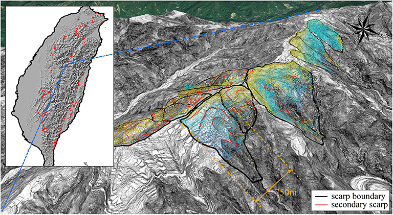
Figure 1. The distribution of the 186 identified potential deep-seated landslide sites in Taiwan (inset panel, Soil Water Conserv. Bureau, 2018), and 10 examples of the scarp boundaries of the potential deep-seated landslides in Ren'-ai Township, Nantou County (Central Geological Survey, 2010). The dots in the scarp areas represent the line-of-sight deformation obtained by using the temporarily coherent point interferometry SAR (TCPInSAR) technique (Chen et al., 2017). Note that the length scale varies according to the 3D perspective.

In traditional geological engineering approaches, the factor of safety of the potential landslide site will then be calculated by using slope stability tools. The most well-known methods are the those based on the limit equilibrium concept, published by Bishop (1955), Mogenstern and Price (1965), and Janbu (1973). In these methods, the slope body above the prescribed failure interface is discretized into a number of vertical slices (free bodies), and a system of algebraic equations is derived according to the force and moment equilibrium, with an additional proposition of internal forces as closure conditions. Because the failure interface is a presumed input parameter in these limit equilibrium methods, there are a few empirical strategies for proposing the interfaces. These strategies include circular, piecewise linear, and other methods, and the choice is made according to the geological condition of the investigated site. The circular failure interface is the most widely employed because this shape is easily parameterizable and agrees with a large portion of common observations. Consequently, automatic iterative search schemes for the least stable interface are implemented in many analysis computation tools (e.g., Siegel, 1978). Once the least stable failure interface is obtained, the landslide depth and 2D volume can be estimated.

Although the analysis is convenient and straightforward, 2D slope stability can be performed on only one or a few heuristically selected representative profiles for each landslide site. Because of this limitation, the analysis may not provide sufficient information for deep-seated landslides in estimating landslide-influenced areas. For this purpose, the 3D scarp depth distribution of the slide mass, for example, is one of the essential quantities required to estimate the runout and spread of the landslide, and it is particularly important for rapid large-scale avalanches, whose motion can be largely influenced by the topographic conditions of the terrain (Kuo et al., 2011; Luca et al., 2016; Tai et al., 2019), and the references therein.

The concept of the factor of safety has long been the key concept in slope stabilization plans. Since the wide deployment of the aforementioned 2D methods, there have also been attempts to extend the slope stability analysis to general 3D terrains. Similar to the 2D limit equilibrium formulation, most of these methods require a priori failure surface; the derived system of equations is a statically indeterminate system, and additional conditions are needed to solve it. For example, in a study by Leshchinsky and Huang (1992a) and Leshchinsky and Huang (1992b), the landslide mass is assumed symmetric and variational optimization is adopted for searching the minimum factor of safety. Ignoring the shear stresses in the internal landslide mass (Ugai, 1985) showed that the failure profile is circular along the sliding direction. A two-directional moment equilibrium method was proposed by Huang and Tsai (2000) and Huang et al. (2002), which can directly determine the sliding direction, instead of presuming a sliding direction. Further improvements are made by including the complete momentum and moment equilibrium conditions (Zheng, 2012; Jiang and Zhou, 2018), in which examples of practical 3D applications are demonstrated. In the group of slope stability analysis methods, Hungr noted that the unbalanced force in the transverse direction of the potential landslide mass is responsible for the errors in the factor of safety (Hungr, 1987; Hungr et al., 1989). In contrast to the limit equilibrium concept, elasto-plastic approach is a full determinant method (Griffiths and Lane, 1999). The adoption of the full determinant method requires more complete underground material parameters and stratigraphic details, such that fitting the failure surface obtained by this type of method to the identified landslide scarp outlines may involve a series of procedural justifications of the material parameters and geological conditions. It has a different mechanical complexity beyond the present consideration and is not pursued further here.

Because the limit equilibrium approach for slope stability analysis yields a statically indeterminant system, additional empirical conditions, the failure surface and internal forces are needed to calculate the factor of safety. Unlike the 2D cases, there is a lack of systematic, convenient and commonly applied ways to form the 3D failure interfaces that fit the observed landslide scarps. However, simple spherical-shaped failure interfaces are often used as illustrative applications in developing 3D slope stability methods (Xing, 1988; Lam and Fredlund, 1993; Huang et al., 2002). Treating spherical surface sections as failure interface elements, a searching scheme has been proposed to construct the regional distribution of the factor of safety (Reid et al., 2000, 2001). Although the method does not focus on finding precise 3D matches of landslide scarps for individual sites, it has become increasingly popular in creating landslide susceptibility maps (Reid et al., 2015; Tran et al., 2018; Zhang and Wang, 2019).

In the examples of the identified potential deep-seated landslide sites in Figure 1, we can see that the scarp areas are identified by the closed polygons and the line-of-sight deformation obtained by using the temporarily coherent point interferometry SAR (TCPInSAR) technique somewhat indicates the landslide activity (Chen et al., 2017). In addition due to the large area that can cover topographic heterogeneous landscapes, each landslide site may contain multiple secondary failure structures, e.g., the cracks and minor scarps in Figure 1 (Central Geological Survey, 2010). In landslide hazard mitigation plans with these types of information, a tool that it is able to generate 3D failure interfaces, conform with the surface scarps and provide related depth information for the landslide mass is required. Such a tool also provides great benefits for landslide sites, of which multiple secondary hazard scenarios are to be studied and managed. Furthermore, with the massive number of 186 potential landslide sites, the tool should be automated so that it can be operated at low costs.

As a tradeoff, the tool is aimed at providing predictions with satisfactory accuracy at small operational efforts but not necessarily with high degrees of precision. In this regard, we propose a simple method for computing the failure interfaces of deep-seated landslides, that is based on the minimization of a smooth surface that encloses a given landslide volume with the specified scarp boundary. The concept arises from the observations that (1), the scarp boundaries of potential deep-seated landslide sites often develop over time and become observable on the surface, for example crown fissures and flank scarps, and (2), landslide volume-area relations can be used to determine the volume from the scarp area. As a result, the average landslide depth is well-constrained, and the 3D failure interface and slide volume can be obtained.

In the proposed method, the geological settings and hydrogeological conditions of each landslide site are neglected. Geological settings include the rock texture, lithological stratas, rock cleavage or joint orientations, etc. These factors affect the intrinsic structure of the failure surfaces and landslide failure pattern. On the other hand, the hydrogeolocal conditions include the rainfall and underground water hydrology, which alter the force balance condition of the slide mass and trigger the landslide. Both geological settings and hydrogeological conditions are site specific details which lead to the deviations of the actual landslide failure surfaces from the predicted. However, to construct these details even for a single site may require extensive resources and investigations such that full coverage surveys and hazard monitoring for a population of landslides become virtually impossible. Under these circumstances, we defer the adoptation of any site specific detail to the present method.

Hence, it is an important task to establish the accuracy baseline of the method in the present paper, such that the paper is organized as follows: A brief introduction to the landslides used in the assessments is presented in section 2; The smooth minimal surface method and statistical assessment indices are described in sections 3 and 4, respectively; the applications of the method to two landslides and two conceptual examples are detailed in section 5 and Appendix 1, respectively, which includes the comparison of the predicted landslide failure interfaces to the actual failure interfaces and calculations of the assessment indices. Then, the application set is extended to include a total of 24 landslides, and their assessment indices are tabulated in section 6. With this amount of data, the accuracy bounds can be inferred.

2. Landslides in the Study Area

In total, 24 deep-seated landslides were selected in the present study (Lin et al., 2011). They were all triggered by the excessive rainfall of the Morakot typhoon and are distributed in three different catchment areas in the southwest mountainous range of Taiwan. The first group, containing 11 sites, is located in the Cishan River catchment area, Jiaxian District, Kaohsiung City, as shown in Figure 2. All these landslides have areas larger than 10 ha, maximum depths over 10 m and, according to the definition from the Taiwanese government, are classified as deep-seated landslides. Among them, the sites labeled with HLIN prefixes are the scarps associated with the Hsiaolin landslides (Kuo et al., 2011; Tsou et al., 2011; Tai et al., 2019). The landslides are defined by using the 2005 and 2010 LiDAR 1 m resolution digital elevation maps (DEMs). The second and third groups of landslides are identified by the DF054 and DF081 prefixes, respectively (Figure 3). DF054 is in the Longjiao River catchment, Dapu Township, Chiayi County, and DF081 is in the Laonung River catchment, Maolin District, Kaohsiung City.

FIGURE 2

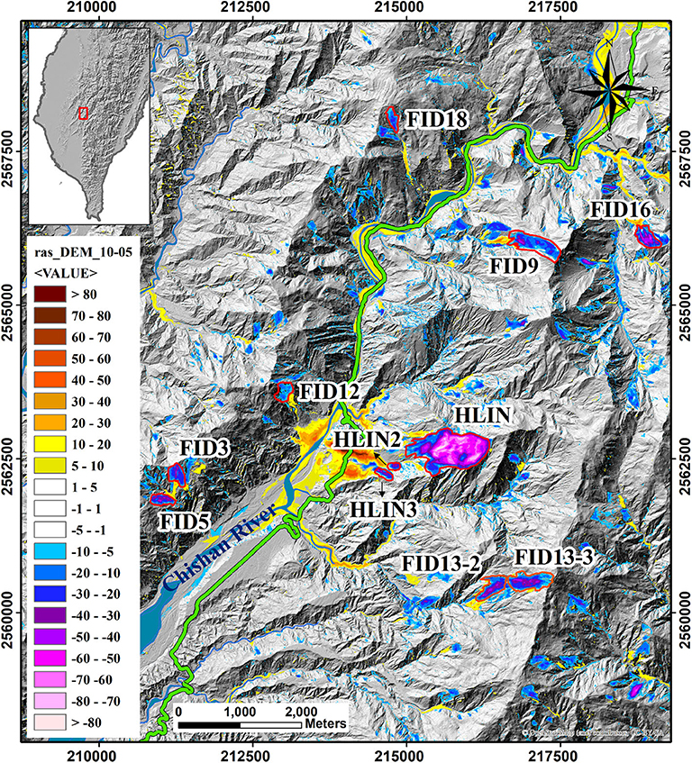
Figure 2. Landslides in the Chishan River catchment, Jiaxian District, Kaohsiung City (Central Geological Survey, 2010). Negative values of the color legends indicate landslide scarp depths and the positive values indicate the deposit thickness in meters. The HLIN prefixes mark the Hsiaolin landslide and its associated landslides. The sites outlined in red solid lines are the deep-seated landslides investigated in the present study. The TWD97 coordinate system is used.

FIGURE 3

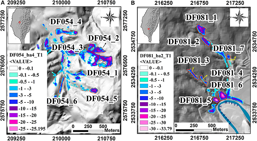
Figure 3. Landslides in (A) the DF054 area, in the Longjiao River catchment, Dapu Township, Chiayi County and (B) the DF081 area in the Laonung River catchment, Maolin District, Kaohsiung City (Central Geological Survey, 2010). Negative values of the color legends indicate landslide scarp depths and the positive values indicate the deposit thickness in meters. The sites outlined in red solid lines are the deep-seated landslides investigated in the present study. The TWD97 coordinate system is used.

The geological structure and stratigraphy of these catchment areas are very briefly reviewed here as background information. Because of space limits, the geological maps of the three catchment areas are relegated to the Supplementary Materials of the paper and are made by referencing (Fei and Chen, 2013). To summarize, the landslide sites of the first group are distributed in three types of surface strata in the Cishan catchment area: Hunghuatzu Formation, Changchihkeng Formation, and Tangenshan Sandstone. These units are arranged chronologically, with the oldest formed in the late Miocene. The landslide sites of DF054 are in the Tangenshan Sandstone and Ailiaochiao Formation (early Pliocene). They consist of sedimentary rocks and are mainly composed of sandstones and shales, in which marine microfossils commonly occur. The third group, the DF081 landslides, is within Chaochou Formation, which is middle Miocene in age and occasionally interlaces with quartzite.

The landslide volumes ($V$) and areas (Ω_p)¹ of the landslides are tabulated in Table 1 and the data are plotted in Figure 4A. In the figure, the regression model is drawn and compared to the well-known equation from Guzzetti et al. (2009) and Klar et al. (2011). It is found that the present 24 landslides agree excellently with the fitted regression line. With these two quantities, we can calculate the equivalent radius: $R$$=\sqrt{{\Omega }_p/\pi }$ ². The characteristic length scale 2$R$, which is the equivalent diameter, will be used as the normalization length factor for statistical quantities varying in the horizontal or slopewise directions, such as the distance of the gravity centers between the actual and predicted landslide volume. In addition, two additional non-dimensional geometric parameters, the roundness 𝔯_r and the sphericity 𝔯_s, can be defined with these measurements and the scarp boundaries.

TABLE 1

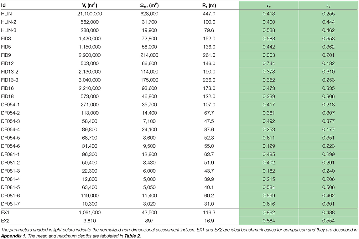
Table 1. Landslide volume, area, equivalent radius, roundness, and sphericity.

FIGURE 4

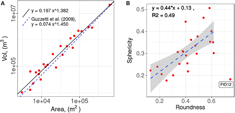
Figure 4. (A) Landslide area and volume relation. (B) Roundness and sphericity relation. The gray area indicates the 95% confidence interval.

We use standard mathematical definitions to define the two parameters. The roundness is defined as the ratio between the radius of the maximum inscribed circle of the scarp and that of the minimum circumscribed circle. Its values range between 0 and 1, with the two extreme values corresponding to an infinitely thin and perfectly circular shapes, respectively. For ellipses, the roundness reduces to the aspect ratio between the width and length. With this analogy, we can associate the roundness to the landslide aspect ratio, which commonly appears in the landslide literature. By adopting this general definition, calculation ambiguities for scarps with complicated shapes can be avoided. On the other hand, the sphericity 𝔯_s is defined as the ratio of the surface area of a sphere of a volume $V$ to the total surface area of the landslide mass $S$₀ + $S$_b (the sum of the free surface $S$₀ and the failure interface areas $S$_b), i.e., ${𝔯}_s={\pi }^{1/3}{(6V)}^{2/3}/(S_0+S_b)$. Its value also ranges from 0, an infinitely thin volume, to 1, a perfect sphere. Because the landslide thickness is usually much smaller than the other spanwise dimensions, the sphericity becomes a factor involving the landslide thickness and the slope³. These two parameters in the above definitions have long been applied in various landslide studies but have different terminologies, such as the width-length ratio and the depth-length ratio (Taylor et al., 2018).

There appears to be a relation between the roundness and sphericity with the present landslide inventory (Figure 4B). The data are somewhat evenly distributed in the range of the roundness and sphericity; i.e., no favorable clustering spots of data are found. Instead, the sphericity generally increases with increasing roundness. Among the sites, FID12 is likely a statistical outlier because of the distinctive gap between it and the other data. Inspecting the site in Figure 2, we find that the scarp boundary of FID12 appears to have a peculiar shape, colloquially a dumbbell shape, with landslide mass biasedly distributed at both end lobes but its relative roundishness reduces the sphericity. The site is likely composed of two distinguished landslides instead of an integrated one. We, however, do not perform further manipulations on this site other than simply exclude it from the accuracy assessments in section 6.

The other important landslide geometric parameters, such as the mean and maximum depths are calculated and listed in Table 2 for facilitating the later accuracy assessments with the failure interface predictions. The related discussion will resume in section 6, after the description of the method of the smooth minimal surface, assessment indices and casewise applications.

TABLE 2

Table 2. DEM grid size, depth-related quantities, and positional offsets of the maximum depth and gravity centers between the predicted and actual scarps.

3. Smooth Minimal Surface

Unlike the full mechanical approach involving fracturing or plasticity, the failure interface is not a determined result but a prescribed prerequisite. Based on observations, circular (2D) or spherical (3D) shaped failure surface profiles are usually applied for slopes with homogeneous and isotropic materials. To fit the application scenario, we relax the surface to a smooth minimal surface. In our application, the minimal smooth surface is obtained by giving an assumed failure volume $V$ with the constraint that its boundary on the free surface matches that from geological field investigations. This type of surface is chosen because it has a close relation to the spherical failure surfaces in 3D slope slability analysis and can degenerate to the spherical surfaces for some special cases, cf. Appendix 1. Therefore it may also inherit the same property that the method fits better for slopes with isotropic and homogenous materials, following the same reasons of the traditional slope stability analysis.

Determining the smooth minimal surface is an optimization process. Let (x, y, z) be the Cartesian coordinates with z vertically pointing upwards, and let the failure interface z_b ≡ z_b(x, y) be a smooth differentiable surface, as shown in Figure 5. Mathematically, the area of the surface can be calculated as

$\begin{array}{ll}S(z_b)={\displaystyle \int }\sqrt{1+\left|\right|\nabla z_b|{|}^2}d{\Omega }_p,& (1)\end{array}$

such that the minimum surface can be acquired by minimizing (1) by varying z_b; i.e.,

$\begin{array}{ll}{S}_b={\displaystyle \underset{z_b}{minS}},& (2)\end{array}$

subjected to the constraints

$\begin{array}{ll}{z}_b=z_0\text{on}\Gamma ,z_b\le z_0\text{in}{\Omega }_p,& (3)\end{array}$

and

$\begin{array}{ll}C(z_b)\equiv {\displaystyle \int }(z_0-z_b)d{\Omega }_p-{V}=0.& (4)\end{array}$

In the equations, ∇ is the 2D gradient operator (∂/∂x, ∂/∂y); Ω_p is the xy−projection area of the failure scarp area; and Γ is the boundary of Ω_p. The first constraint states that the boundary elevation of the failure interface is equal to the elevation of the free surface, z₀ ≡ z₀(x, y); the scarp surface is below the free surface; and the second constraint states that the failure volume is the prescribed volume V.

FIGURE 5

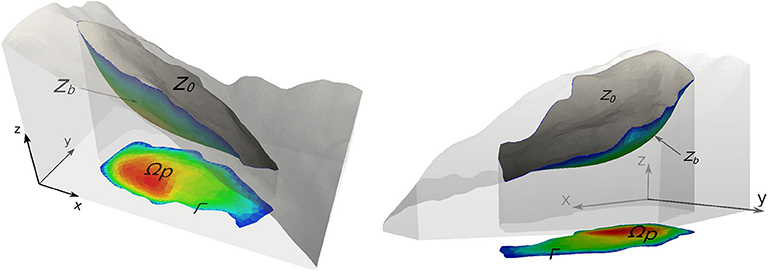
Figure 5. Conceptual sketch, symbols, and coordinate system. The landslide site FID5, defined in Figure 2 is used as an example. Symbols z₀ ≡ z₀(x, y) and z_b ≡ z_b(x, y) are the free surface and underground failure interfaces, respectively. Ω_p and Γ are the projection of the scarp area and outline on the xy plane, respectively. The scarp failure interfaces and depth are largely exaggerated for clarity in this sketch, and the color map conceptually indicates the scarp depth.

The scheme is implemented in the open source finite element platform FreeFEM++, ver. 3.47 (or above) (Hecht, 2012), and the integrated Interior Point OPTimizer (IpOpt, Wächter and Biegler, 2006) optimization scheme in FreeFEM++ is applied to find the numerical solution. In the scheme, the Jacobian and Hessian matrices of the target function (1) are used to accelerate the numerical convergence:

$\begin{array}{ll}{S}^{\prime }(z_b)·[{\widehat{z}}_b]={\displaystyle \int }\frac{\nabla z_b·\nabla {\widehat{z}}_b}{\sqrt{1+\left|\right|\nabla z_b|{|}^2}}d{\Omega }_p,& (5)\end{array}$

and

$\begin{array}{l}{S}^{\prime \prime }(z_b)·([{\widehat{z}}_b],[{\check{z}}_b])={\displaystyle \int (\frac{\nabla {\widehat{z}}_b·\nabla {\check{z}}_b}{{(1+||\nabla z_b|{|}^2)}^{1/2}}}\\ -\frac{(\nabla {\check{z}}_b·\nabla z_b)(\nabla {\widehat{z}}_b·\nabla z_b)}{{(1+||\nabla z_b|{|}^2)}^{3/2}})d{\Omega }_p.& (6)\end{array}$

The above two expressions are written with the help of the notation of the Fréchet derivative for facilitating the numerical scheme implementation (Vergez et al., 2016). Similarly, the Jacobian matrix of constraint (4) is

$\begin{array}{ll}C\prime {}^{}(z_b)·\left[{ẑ}_b\right]=-{\displaystyle \int }d{\Omega }_p=-{\Omega }_p.& (7)\end{array}$

Equations (5), (6), and (7) are evaluated at discrete points in each mesh element. Supporting external C++ functions are coded to handle the DEM, scarp boundary outline inputs and outputs to other software for geographic information systems (GIS), such as ArcGIS, qGIS, and GRASS. Initially, the outline is uniformly discretized with a prescribed number into a set of linear edges, and the mesh of the scarp area is generated. Then, the optimization (2) for the minimal surface is executed. Depending on the precision requirement of the mesh, multiple passes of mesh adaptation can be performed based on the calculated failure interface.

As seen in the formulation and calculation principle, the smooth minimal surface can be equivalently replaced with other mathematical surfaces, provided that they are phenomenologically reasonable and their descriptive expressions are available. It is also in principle possible to design transformations that can further manipulate the predicted failure surfaces to incorporate with site specific geological settings or hydrogeological conditions. Nevertheless, because the method is a phenomenological approach, the accuracy of the failure surface prediction has to be verified with actual landslide data. In what follows, we use the current smooth minimal surface to proceed the application example and accuracy assessment. The assessment indices and procedure are generic and applicable to future alternative failure surface prediction or transformation schemes.

4. Assessment Indices

The proposed prediction method for the failure interface is purely mathematical. Intuitively, the failure interface is mimicked by a “soap-bubble” film that encloses the free surface at a specified volume $V$. Because the film is uniquely defined, it becomes important to assess the fitness, i.e., the closeness between the film and the real failure interface and to establish the error bounds of the method.

Under the current approach, the area, volume and scarp boundary are kept identical for each landslide, and hence, the mean depth of the predicted landslide mass will be equal to the actual one, ($V$/Ω_p), in principle. Nevertheless, because of the nature of discrete numerical data and computations, the discretization incurs digital errors, e.g., the DEM is presented at a resolution of grid size Δ and in the minimal surface calculation, forward and backward interpolation is performed between the DEM and mesh system. It is expected that this type of error is bounded by the precision of the mesh, such that we list the normalized grid size $\bar{\Delta }$ as an informative indicator, which is normalized with respect to the equivalent diameter 2$R$.

To compare the predicted and actual failure interfaces, we start by calculating and finding the crucial quantities in each of them: the mean and maximum scarp depths (h_mean and h_max, respectively) and the positions of the gravity center r_GC and maximum depth point r_MD. One can define the measures of discrepancy as the differences of these quantities between the predicted and actual landslide failure interfaces. To eliminate the landslide scale effect, the depthwise quantities are normalized with respect to the actual mean depth; i.e., ${\bar{\epsilon }}_{\text{mean}}=(h_{\text{mean}}^{\text{pred}}-h_{\text{mean}}^{\text{act}})/h_{\text{mean}}^{\text{act}}$, ${\bar{\epsilon }}_{\text{max}}=(h_{\text{max}}^{\text{pred}}-h_{\text{max}}^{\text{act}})/h_{\text{mean}}^{\text{act}}$, and the spanwise offsets of the gravity centers d_GC and maximum depths d_MD are then normalized with respect to the equivalent diameter; i.e., ${\bar{\epsilon }}_{\text{GC}}=d_{\text{GC}}/(2R)=|{\text{r}}_{\text{GC}}^{\text{pred}}-{\text{r}}_{\text{GC}}^{\text{act}}|/(2R)$, ${\bar{\epsilon }}_{\text{MD}}=d_{\text{MD}}/(2R)=|{\text{r}}_{\text{MD}}^{\text{pred}}-{\text{r}}_{\text{MD}}^{\text{act}}|/(2R)$. The superscripts ^pred and ^act obviously represent the model predictions and the actual measurements of these quantities. ${\bar{\epsilon }}_{\text{mean}}$ contains only the discretization error as discussed previously. ${\bar{\epsilon }}_{\text{GC}}$ and ${\bar{\epsilon }}_{\text{MD}}$ somewhat represent the bias of the depth distributions between the predicted and actual failure interfaces.

The ratio ${\bar{\epsilon }}_{max}$ is one of the assessment indices, which merely measures the difference between the maximum depths. The other assessment indices are the statistical properties associated with the prediction discrepancy. Let the prediction discrepancy be the difference between the actual and predicted scarp depths, $\delta (x,y)=h^{\text{act}}-h^{\text{pred}}=z_b^{\text{pred}}-z_b^{\text{act}}$, where (x, y) ∈ Ω_p. The statistical properties that can be computed include the distribution function of the prediction discrepancy δ, its mode(δ) (the most frequent discrepancy), standard deviation std(δ), and their non-dimensionalized counterparts, ${\bar{\epsilon }}_{\text{mode}}$ and ${\bar{\epsilon }}_{\text{std}}$ (normalized with respect to $h_{\text{mean}}^{\text{act}}$). Note that std(δ) is virtually the root mean square error (RMSE) between the predicted and actual depths according to its computational principle (Kuo et al., 2011). For completeness, the linear regression model, $h^{\text{act}}=\bar{\beta }{h}^{\text{pred}}+\alpha$, is also calculated for each landslide site. To facilitate comparisons among landslides of different size scales, the intercept α of the regression model is again non-dimensionalized with respect to $h_{\text{mean}}^{\text{act}}$; i.e., $\bar{\alpha }=\alpha /h_{\text{mean}}^{\text{act}}$. Together with the slope $\bar{\beta }$ and the coefficient of determination R², these regression parameters are tabulated in Table 3.

TABLE 3

Table 3. The modes, standard deviations of the prediction discrepancy δ(x, y), resultant regression parameters, and SSIMs.

The aforementioned statistical quantities are commonly applied in landslide studies. The limitations of these indices are that they rely on the fitness of a single point (e.g., ${\bar{\epsilon }}_{\text{max}}$, ${\bar{\epsilon }}_{\text{MD}}$), on the averaged properties of the scarp (${\bar{\epsilon }}_{\text{mean}}$, ${\bar{\epsilon }}_{\text{GC}}$), or on the discrepancy distribution of the scattered grid data (${\bar{\epsilon }}_{\text{mode}}$, ${\bar{\epsilon }}_{\text{std}}$, $\bar{\alpha }$, $\bar{\beta }$, R², etc.). To the authors' point of view, one important factor has not yet been properly addressed by these indices, and this factor is the likelihood of the patterns between the predicted and actual scarps. The pattern refers to the landslide depth distribution in the proximity of any given point in the scarp area, and this pattern is highly dependent on the neighboring area. The patterns are omitted in the former statistical indices because the elevation of each mesh grid is treated as an independent random variable.

To include in the spatial topographic patterns into the current assessment, we adopt the so-called structural similarity index (SSIM), which was developed for and is commonly used in image studies for assessing qualities among various image-processing schemes (Wang et al., 2004). In the computation of this index, the value of each pixel of the image, or here, those of the grids in the scarp area, is replaced by the SSIM calculated in the vicinity window (grid) surrounding the pixel. For each window, the SSIM is defined as

$\begin{array}{ll}\text{SSIM}(h^{\text{act}},h^{\text{pred}})=l(h^{\text{act}},h^{\text{pred}})c(h^{\text{act}},h^{\text{pred}})s(h^{\text{act}},h^{\text{pred}}),& (8)\end{array}$

where the functions on the right hand side are defined as

$\begin{array}{lll}l(h^{\text{act}},h^{\text{pred}})& =& \frac{2h_{\text{mean}}^{\text{act}}{h}_{\text{mean}}^{\text{pred}}+C_1}{{h_{\text{mean}}^{\text{act}}}^2+{h_{\text{mean}}^{\text{pred}}}^2+C_1},\\ c(h^{\text{act}},h^{\text{pred}})& =& \frac{2h_{\text{std}}^{\text{act}}{h}_{\text{std}}^{\text{pred}}+C_2}{{h_{\text{std}}^{\text{act}}}^2+{h_{\text{std}}^{\text{pred}}}^2+C_2},\\ s(h^{\text{act}},h^{\text{pred}})& =& \frac{{\sigma }^{\text{act},\text{pred}}+C_2/2}{h_{\text{std}}^{\text{act}}{h}_{\text{std}}^{\text{pred}}+C_2/2}.& (9)\end{array}$

The symbols in the expressions are slightly modified to be consistent with those in the current work, such that $h_{\text{std}}^{\text{act}}$, $h_{\text{std}}^{\text{pred}}$ and σ^{act, pred} are the standard deviations of the actual and predicted scarp depths, respectively, and the cross variance ${\sigma }^{\text{act},\text{pred}}=\left\{\int (h^{\text{act}}-h_{\text{mean}}^{\text{act}})(h^{\text{pred}}-h_{\text{mean}}^{\text{pred}})d{\Omega }_p\right\}/{\Omega }_p$. C₁ and C₂ are small constant parameters that stabilize the expressions for small denominators and their default values, as well as the window, are taken from Wang et al. (2004). The three expressions in (9) are for comparing the luminance, contrast and structural pattern in image studies but can be analogous to the comparison of the landslide scarp depth, the change in the depth and the pattern of the depth in the present study. Therefore, the SSIM should perform similarly as an assessment index to evaluate the fitness of the prediction. In the implementation, the SSIMs in the vicinity area of each grid are calculated with the help of the standard Gaussian window functions of signal processing and statistics. The window size is 10 DEM grids. The resultant SSIM for each landslide site is then defined as the average SSIM over the scarp area and takes a value between 0 and 1, where 0 indicates complete dissimilarity and 1 indicates perfect identicalness. Tests showed that the resultant SSIM does not sensitively depend on the window size and function. For further statistical theories and derivation details, interested readers are directed to the referenced literature.

5. Application Examples: FID5 and FID18

In this section, application examples of the minimal surface method for two landslides are presented. There are also two additional benchmark cases for validating the minimal surface optimizations, but because of their simplicity, these benchmark cases are relegated to Appendix 1. The two real cases, one with a good prediction and the other with a fair prediction, are chosen and they are purposely selected to illustrate the comparison of the opposite predictions. The calculation of the statistical assessment indices are also explained in detail, particularly those operational procedures that are not thoroughly described in section 3 and section 4.

We start with the FID5 landslide. The FID5 site is on the slope of the west bank of the Cishan River and has a volume $V$ of 1,167,000 m³ and an average slope of 35.2°, inclined toward the E-NE direction. The DEM domain is 600 × 340 m, in the x and y directions, respectively, with a resolution of 20 m (normalized to $\bar{\Delta }=7.36\%$). The 3D view of the site has been shown as a conceptual sketch in Figure 5. The post-landslide topography as well as the scarp boundary is plotted in Figure 8A. The projection area, Ω_p, of the scarp is then equal to 58, 000 m² and the equivalent radius $R$ = 136.0 m. These geometric dimensions lead to a roundness ratio 𝔯_r of 0.442 and a spherical ratio 𝔯_s of 0.362.

As the slope and scarp boundary are now defined, we proceed with the preparation of the input data set of the minimal surface optimization scheme. Because FreeFEM++ only provides unstructured triangular meshing for general shapes of computational domains, numerical interpolation algorithms are employed to convey the data between the structured DEM mesh and the unstructured FreeFEM++ computational grids. We do not have any compulsory reasons to adopt higher order accuracy interpolations for the present purpose; thus only first order interpolation algorithms are used.

When the DEM and scarp outline are input, parsed and interpolated, an initial unstructured mesh for the scarp domain Ω_p is constructed⁴. The P2 finite elements are used for data arrangement and manipulation. Then, the optimization routine for the minimal surface is executed. To extend the scarp prediction to future mechanical slope stability analyses, which may require a higher accuracy within the FreeFEM++ framework, we perform a second-pass mesh adaptation based on the scarp depth of the initial calculation with a mesh refinement precision error factor of 0.05⁴. The refined mesh for the smooth minimal surface calculation is superposed in Figure 6A. A high mesh density is found in the areas where the topography exhibits large variations, in this case, around the vicinity of the ridges and edges of the slope surface. After the smooth minimal surface is found, it is interpolated back to the structured DEM grids.

FIGURE 6

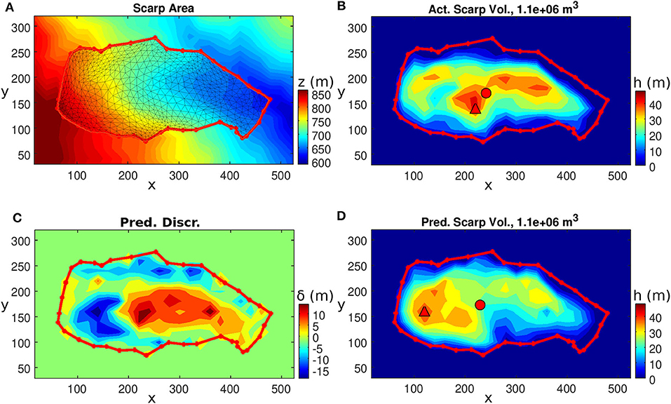
Figure 6. Landslide FID5. Clockwise from the upper-left figure: (A) The topography, scarp outline and smooth minimal surface computational mesh. (B) The actual landslide depth. (C) The predicted landslide depth. (D) The prediction discrepancy δ(x, y). The solid red circle and triangle represent the gravity center and maximum depth location, respectively.

The actual and predicted landslide depths are shown in Figures 6B,C. The landslide has a maximum depth $h_{\text{max}}^{act}$ of 47.4 m and a mean depth $h_{\text{mean}}^{act}$ of 21.2 m. Their predicted counterparts are $h_{\text{max}}^{pred}=40.6$ m and $h_{\text{mean}}^{pred}$ 21.2 m, respectively. These values lead to dimensionless discrepancies ${\bar{\epsilon }}_{\text{max}}=32.40\%$ and ${\bar{\epsilon }}_{\text{mean}}=0.40\%$, respectively. The prediction discrepancy distribution δ(x, y) is plotted in Figure 6D. The prediction overestimates the scarp depth in the part of the slope with higher elevation, such that δ(x, y) has two major oppositely signed zones aligned adjacently along the downslope direction. This distribution of δ(x, y) leads to the positions of both the maximum depth and gravity center of the landslide mass residing on the upper-slope side compared to the actual landslide mass. The positional offsets of the maximum depth and gravity center are d_MD = 102.0 m (${\bar{\epsilon }}_{\text{MD}}=37.53\%$), and d_GC = 11.3 m (${\bar{\epsilon }}_{\text{GC}}=4.17\%$).

The histogram of the prediction discrepancy δ(x, y) is plotted in Figure 7A. It depicts the frequency distribution of δ(x, y), and the distribution has an approximate symmetric triangular shape except for a minor peak at δ ≈ −9 m. Its mode, mode(δ), is approximately −0.7 m and the standard deviation, std(δ) is 7.3 m, leading to normalized discrepancy ratios of ${\bar{\epsilon }}_{\text{mode}}=3.51\%$ and ${\bar{\epsilon }}_{\text{std}}=34.51\%$. In Figure 7B, the scattered data of h^pred and h^act are plotted in the regression analysis and the resultant linear regression line is h^act = 0.916h^pred+1.84, which provides the normalized intercept parameter $\bar{\alpha }=0.087$. The coefficient of determination, R², is 0.618. The SSIM is 0.864, which is one of the cases with a high score, cf. section 6. In the SSIM computation, the default Gaussian window, of size 11 × 11 with a standard deviation of 1.5 cell sizes, is used. To compare with other cases, these statistical quantities are tabulated in both Tables 2, 3.

FIGURE 7

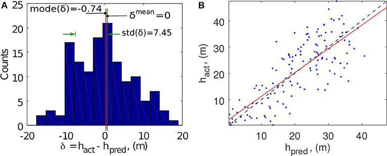
Figure 7. Landslide FID5. (A) Histogram of δ(x, y), the graphical definition of mode(δ), std(δ) and the negligible mean depth discrepancy δ^mean. (B) Scatter plot and regression analysis of the predicted and actual depths.

FID18 is a landslide site near the Zion village. The landslide has a volume of 567,000 m³, an area of 46,800 m², a maximum depth of 31.3 m, and a slope of 29.4° inclined toward the south. The roundness and sphericity are 0.339 and 0.306, respectively. The DEM has a spatial resolution of 20 m ($\bar{\delta }=8.19\%$). After performing the smooth minimal surface calculation, the computational mesh, the actual, predicted depths and the prediction discrepancy are plotted in Figure 8. The panels are arranged the same way as in the previous FID5 case. Interestingly, the prediction also overestimated the landslide depth in the upper part of the slope and underestimated the lower part of the slope. Therefore, the prediction discrepancy also shows similar negative-positive-lobed prediction discrepancy zones along the downslope direction as in the previous case.

FIGURE 8

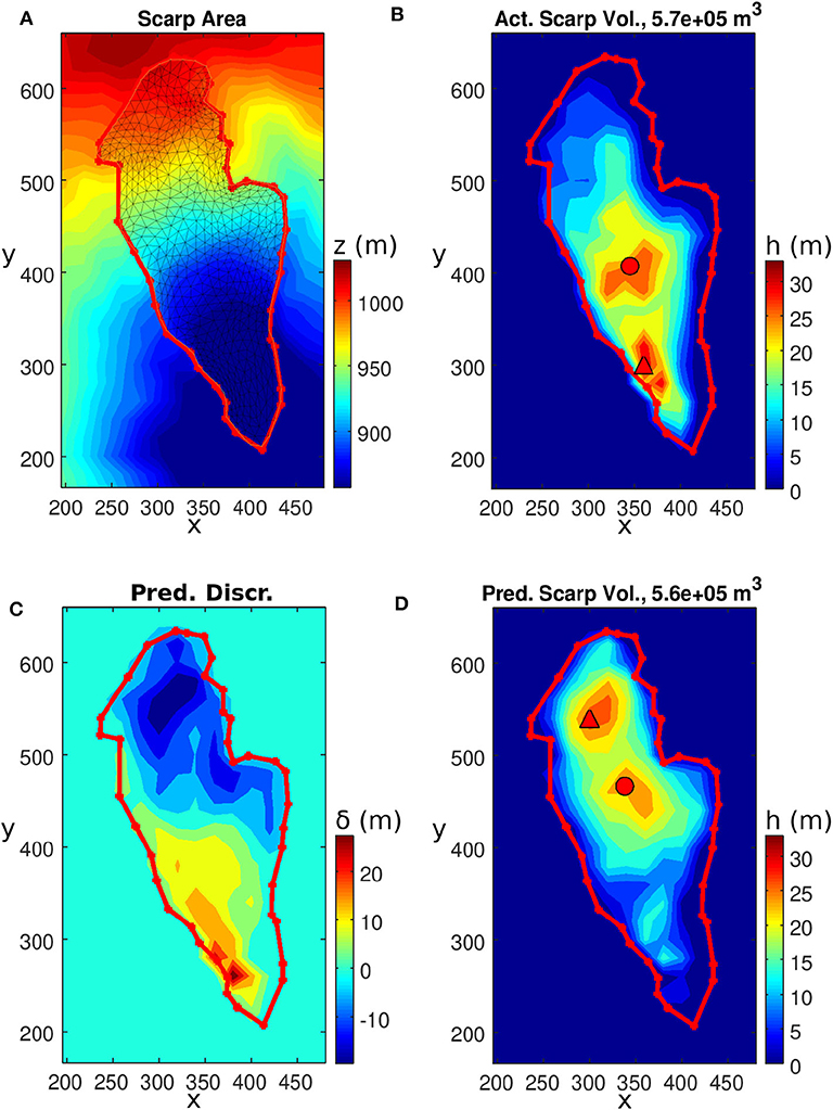
Figure 8. Landslide FID18. Clockwise from the upper-left figure (A) The topography, scarp outline and smooth minimal surface computational domain. (B) The actual landslide depth and scarp outline. (C) The predicted landslide depth. (D) The prediction discrepancy δ(x, y). The solid red circle and triangle represent the gravity center and maximum depth location, respectively.

The accompanied discrepancy histogram and regression analysis are shown in Figure 9. The histogram indicates that the discrepancy has a flatter distribution with a few more irregular minor peaks than that of FID5. This case is identified as a poorer fit because the prediction also has relatively poor linear regression parameters compared to the actual data: the intercept $\bar{\alpha }$ (0.72, normalized with respect to $h_{\text{mean}}^{\text{act}}$) is large, $\bar{\beta }$ (0.28) deviates greatly from 1, and R² (0.063) is low. We found consistent indications from ${\bar{\epsilon }}_{\text{mode}}$ (52.47%), ${\bar{\epsilon }}_{\text{std}}$ (71.61%) and ${\bar{\epsilon }}_{\text{GC}}$ (44.44%), representing larger prediction discrepancies, wider deviations and larger offsets of the gravity center. The SSIM (0.677) also has one of the lowest scores. Nevertheless, despite these comparatively subnormal indices, the prediction is only 2.31% for ${\bar{\epsilon }}_{\text{mean}}$ and a satisfactory 20.61% for ${\bar{\epsilon }}_{\text{max}}$, as both the scarp area and volume are constrained in the present failure surface prediction method such that the mean depth has interpolation errors only and the maximum depth is generally proportional to the mean depth (see section 6).

FIGURE 9

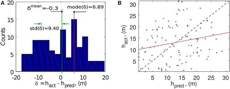
Figure 9. Landslide FID18. (A) Histogram of δ(x, y) and the graphical definition of mode(δ), std(δ) and the negligible mean depth discrepancy δ^mean. (B) Scatter plot and regression analysis of the predicted and actual depths.

6. Deployment to the Full Set of Landslides and Assessments

The method is applied to the 24 landslide sites defined in Figures 2, 3 and Table 1. The resolution of the DEMs varies from 5 to 20 m due to various preparation conditions, such as public release policies and the size of landslide sites. Though with these different resolution settings, the normalized grid size $\bar{\Delta }$ remains within 10% (Table 2). In the same table, the maximum and mean depths as well as the positional offsets of the maximum depths and gravity centers between the actual and predicted scarps are listed. To make visual comparisons, the depth-related quantities are plotted in Figure 10. The predicted and actual depths excellently match the diagonal lines in Figure 10A. Reorganizing the data, we find that there is also a linear relationship between the maximum and mean depths (Figure 10B). From the regression model, we have a gross guideline that the maximum scarp depth can be obtained by multiplying the mean scarp depth by a factor of 2.3.

FIGURE 10

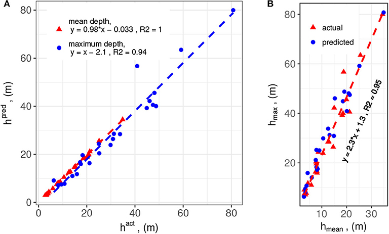
Figure 10. Combined comparison between (A) the predicted and actual depths, and (B) the maximum and mean depths. The data sources and regression relations are marked in the figure legends.

The remaining assessment indices (i.e., the mode, standard deviation, regression parameters of the prediction discrepancy and the SSIM) are tabulated in Table 3. To comprehend at a glance the interrelationship among the assessment indices, we draw the box plots of the normalized indices in Figure 11. These indices are sorted in ascending order by their median values and are divided into two groups, of which the first group contains the slopewise quantities, normalized by 2$R$ and the second involves the depth-related quantities, normalized by $h_{\text{mean}}^{act}$. The discretization is determined by the DEM resolution, $\bar{\Delta }$, and its values in Figure 11A, are within 10% for the present data-sets. The values of the normalized mean prediction discrepancy, ${\bar{\epsilon }}_{\text{mean}}$ in Figure 11B, are small and are all within 10%, as expected. As argued in section 4, this finding is due to ${\bar{\epsilon }}_{\text{mean}}$ being constrained by the specified area and volume inputs to the method and the small values arise from the DEM discretization approach and interpolation scheme.

FIGURE 11

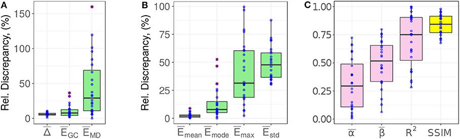
Figure 11. Box plots for the assessment indices (A) $\bar{\Delta }$, ${\bar{\epsilon }}_{\text{GC}}$ and ${\bar{\epsilon }}_{\text{MD}}$, (B) ${\bar{\epsilon }}_{\text{mean}}$, ${\bar{\epsilon }}_{\text{mode}}$, ${\bar{\epsilon }}_{\text{max}}$, and ${\bar{\epsilon }}_{\text{std}}$, and (C) $\bar{\alpha }$, $\bar{\beta }$, R² and the SSIM. The normalization parameters are 2$R$ for the first group and $h_{\text{mean}}^{\text{act}}$ for the second group.

There are two assessment indices associated with the maximum scarp depth: the positional offset ${\bar{\epsilon }}_{\text{MD}}$ and discrepancy ${\bar{\epsilon }}_{\text{max}}$. The two indices both exhibit much larger spreads of their data values than the other indices. The positional offset of the gravity centers of the predicted and actual scarps is interestingly small approximately 6% (median value), dimensionally of 6%·2$R$ ≈ 0.12$R$. An important implication of this fact for future incorporation of the mechanical slope stability analysis is that the force balance condition of the predicted scarp mass (cf. free body diagram) may not significantly differ from the actual mass, and consequently, the landslide motion dynamics may bear a close similarity. Research into this proposition is beyond the scope of the present paper and will be reported in follow-up studies.

The index ${\bar{\epsilon }}_{\text{mode}}$ depicts the most frequent prediction discrepancy, and from this definition, it somewhat indicates the skewness of the frequency distribution of δ(x, y), cf. Figures 7, 9. The moderate value range of ${\bar{\epsilon }}_{\text{mode}}$ (Figure 11B) suggests that the frequency distributions of the δ(x, y) histograms remain reasonably symmetric. As mentioned in section 4, the standard deviation index ${\bar{\epsilon }}_{\text{std}}$ equivalently describes the RMSE between the predicted and actual scarps. The box plot shows that the deviation is approximately 45 ± 10% of the mean scarp depth, or approximately 19 ± 4% of the maximum scarp depth, based on the regression model depicted in Figure 10B. These margins of ${\bar{\epsilon }}_{\text{std}}$ indicate that the present smooth minimal surface is satisfactory for predicting the landslide failure interfaces. Figure 11C presents the value range of the resultant regression parameters and the SSIM.

Finally, we comment on whether there is a relationship between the good predictions from the present method and the landslide scarps. The importance of the answer to this question is that it enables us to estimate the goodness of the prediction without needing to know the actual underground failure interface when the method is applied to hazard mitigation plans for potential landslide sites. For this purpose, the roundness is chosen as the parameter to describe the landslide scarp because this parameter is usually the first obtainable information from topographic surveys. After reviewing the collection of the assessment indices, we select ${\bar{\epsilon }}_{\text{std}}$, R² and the SSIM to measure the fitness of the predictions. These three indices vs. the roundness are plotted in Figure 12. The locally estimated scatterplot smoothing (LOESS) technique (Cleveland et al., 1992), is then applied to determine their relationships with certain degrees of statistical confidence. One exception is made for the noted outlier FID12, cf. section 2, which is excluded from the LOESS analysis but is included in the figure for reference.

FIGURE 12

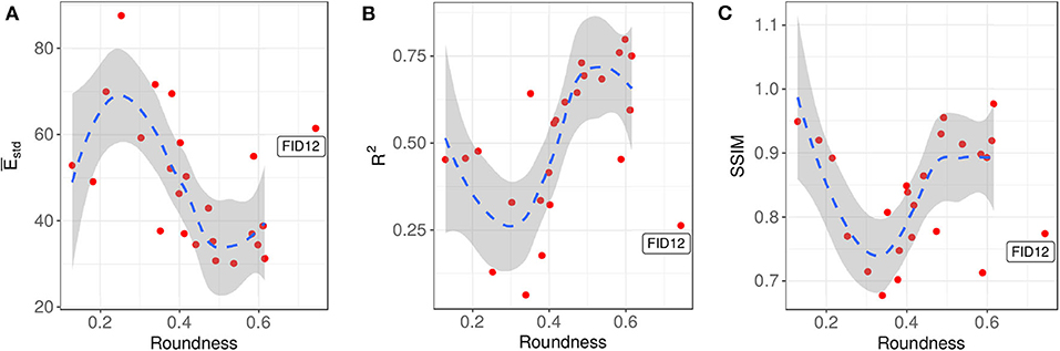
Figure 12. Three selected normalized assessment indices vs. the landslide scarp roundness. The roundness vs. (A) ${\bar{\epsilon }}_{\text{std}}$, (B) R², and (C) the SSIM. The dashed lines are obtained by LOESS regression, with a default span parameter of 0.75 (Cleveland et al., 1992). The gray shaded areas indicate 95% confidence intervals. FID12 is an outlier and is excluded from the regression analysis.

Comparing the three LOESS results, we can draw a consistent conclusion that the smooth minimal surface performs relatively poorer for a roundness of approximately 0.3. At this value, the standard deviation ${\bar{\epsilon }}_{\text{std}}$ (RMSE) has the highest value whereas the coefficient of determination R² and structural similarity index SSIM have the lowest values. For values away from a roundness of 0.3, the landslide scarp becomes either slenderer or more circular. Intuitively, these two regimes have lower geometric complexity because they both degrade to simpler 2D-like scarps. The prediction fitness may thus be associated with the reduction in the geometric complexity. In fact, the same conclusion can be reached with the undiscussed $\bar{\alpha }$ and $\bar{\beta }$ parameters.

A note to keep in mind is that the conclusion drawn from the above assessments is based on the current simple smooth minimal surface approach for the failure surfaces. The geological settings and hydrogrological conditions are completely omitted. This arrangement is deliberate because it is essential at present to construct a baseline dataset with the simplest setting of the method. The dataset will be the foundation for future comparative studies if alternative failure surface prediction strategies are proposed. For example, the dataset will be used for improvement assessments when we design mathematical transformations to manipulate the failure surface predictions to accommodate site specific geological conditions. On the other hand, whether the current approach fits better for landslides in slopes with uniform rocks also remains to be investigated and the hypothesis can be examined by comparing to the baseline dataset. These related studies will be reported in upcoming papers.

7. Conclusion

Even with protection targets, a large number of potential deep-seated landslides in the mountain ranges were identified in a series of renewed hazard mitigation initiatives in Taiwan. When implementing successful, detailed hazard mitigation strategies, tasks such as the determination of the landslide influencing areas and the installation of a monitoring system, need the estimation of the landslide volumes, failure interfaces and other related information. Having observed that these deep-seated landslide sites are represented by polygons in the GIS and that there are regression relations between the landslide scarp areas and volumes, we propose to use smooth minimal surfaces to approximate the landslide failure interfaces. The smooth minimal surface is constructed by minimizing the surface area while keeping the enclosed volume fixed at the value obtained by the scarp area-volume relation. This type of surfaces is chosen because it is closely related to the commonly used spherical-shaped surfaces in slope stability analyses. Consequently, it is expected that the prediction may suit better for slopes with homogeneous and isotropic rocks.

The method, though still in its primitive form, has the potential to be applied to hazard mitigation plans in which higher tolerance in prediction errors is allowed. Therefore, one of the main themes of the paper is to establish the knowledge about the fitness and margins of errors for this method setting. The fitness of the prediction results was verified with 24 landslides that were triggered by excessive rainfall during the 2009 Morakot typhoon. A collection of assessment indices was reviewed and among these indices, the standard deviation ${\bar{\epsilon }}_{\text{std}}$ (equivalently, the RMSE), the regression parameters and the SSIM are shown to contain the information about the prediction discrepancy over the entire scarp domain for each landslide site. Using the present landslide dataset, the value range of the index ${\bar{\epsilon }}_{\text{std}}$ was found to be approximately 45 ± 10% of the mean scarp depth. The limited positional offset of the gravity center, ${\bar{\epsilon }}_{\text{GC}}$, indicates that the force balance condition may not significantly differ from the actual landslide mass. Finally, the relation between the prediction fitness and scarp geometry was determined: Better predictions are achieved for either slender or comparatively circular scarps. Overall, the indices reveal that the smooth minimal surface method is able to produce practical, acceptable predictions of deep-seated landslide failure interfaces, despite the omission of stratigraphy, geological structures and hydrogeological conditions.

The method is implemented with ease of use in mind such that operational costs are kept low and automation processes for a large number of landslide sites can be made possible. An additional benefit is that the method can simultaneously generate 3D computational meshes for the landslide scarp mass. These meshes can be applied to many subjects related to hazard mitigation plans. For example, for slope stability management, it is currently ongoing to develop 3D extended schemes for landslide volume and safety factor relations. Integrating with surface deformation data and material constitutive laws, slip displacements on the failure surface can be inversed for deep-seated landslides, in a somewhat similar way to dislocation model in tectonics. The volumetric mesh, or depth distribution, can also be used as the initial mass to perform landslide motion simulation to assess the influenced area. Summarizing the abovementioned potential applications and verification details presented in the present paper, we draw a combined flowchart in Figure 13 for the two application scenarios of the method. The inputs and products of the method are explicitly indicated for each application scenario.

FIGURE 13

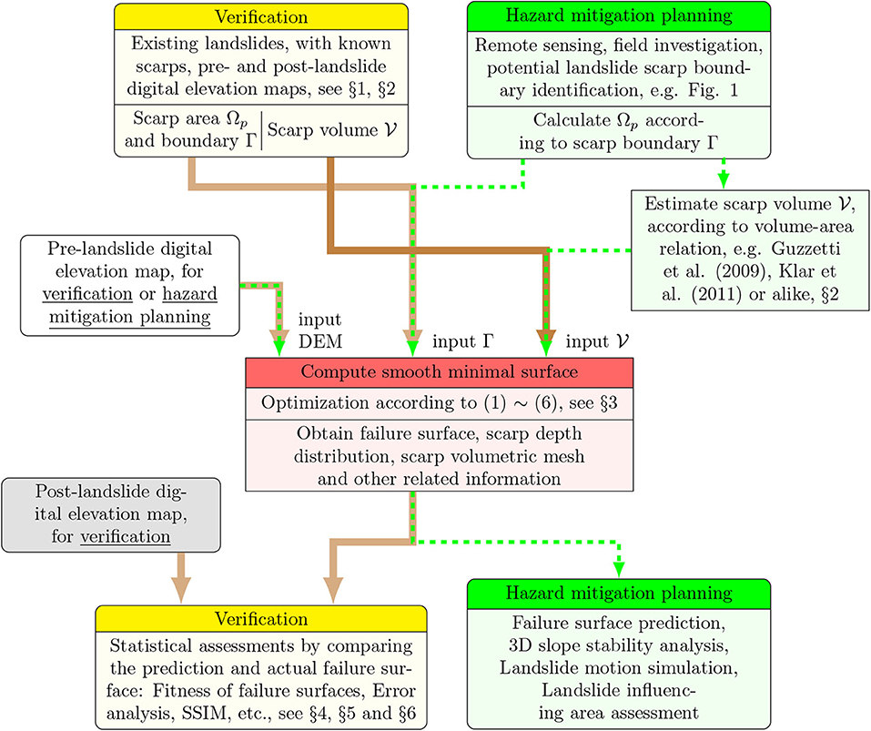
Figure 13. Flowchart of the present model for both application scenarios: verification, blocks shaded in light yellows, and hazard mitigation planning, blocks in light greens. The current failure surface prediction model is in light red colors. For failure surface prediction verification, i.e., the main theme of the paper, the computational flow is led by the thick solid brown lines but, for hazard mitigation planning, it is led by the thin dashed green lines.

Data Availability Statement

All datasets and computational codes generated for this study are included in the article/Supplementary Material.

Author Contributions

All authors listed have made a substantial, direct and intellectual contribution to the work, and approved it for publication.

Funding

This work was supported in parts by grant no. MOST-106-2625-M-001-001- from the Ministry of Science and Technology and grant no. SWCB-108-10.10.1-S4 from the Soil and Water Conservation Bureau, of Taiwan, Republic of China.

Conflict of Interest

The authors declare that the research was conducted in the absence of any commercial or financial relationships that could be construed as a potential conflict of interest.

Acknowledgments

The authors thank Dr. Liu, Shou-Heng, Mr. Chen, and Yi-Zhong for their preparations of the DEMs and discussions.

Supplementary Material

The Supplementary Material for this article can be found online at: https://www.frontiersin.org/articles/10.3389/feart.2020.00211/full#supplementary-material

Footnotes

1. ^In common geological practice, Ω_p is measured on the horizontal projection of the landslide scarp, cf. Figure 5.

2. ^$R$, thus, is also defined on the horizontal projection plane, cf. Figure 5.

3. ^Under the shallowness assumption, the total surface area $S$₀+$S$_b is approximately 2Ω_p divided by the directional cosine of the slope.

4. ^By BAMG, bidimensional anisotropic mesh generator with mesh refinement facility, integrated in FreeFEM++.

References

Baroň, I., Řehánek, T., Vošmik, J., Musel, V., and Kondrová. (2011). Report on a recent deep-seated landslide at gírová mt., czech republic, triggered by a heavy rainfall: The gírová mt., outer west Carpathians; Czech Republic. Landslides 8, 355–361. doi: 10.1007/s10346-011-0255-y

CrossRef Full Text | Google Scholar

Bishop, A. W. (1955). The use of slip circles in the stability analysis of slopes. Geotechnique 5, 7–17. doi: 10.1680/geot.1955.5.1.7

CrossRef Full Text | Google Scholar

Cardinali, M., Paola, R., Guzzetti, F., Ardizzone, F., Antonini, G., Galli, M., et al. (2002). A geomorphological approach to the estimation of landslide hazards and risks in Umbria, Central Italy. Nat. Hazards Earth Syst. Sci. 2, 57–72. doi: 10.5194/nhess-2-57-2002

CrossRef Full Text | Google Scholar

Central Geological Survey (2010). Generation and QA/QC of LiDAR DEM in Heavy Disaster Area Induced by Typhoon Morakot in 2009 (in Chinese). Technical report, Cent. Geol. Survey Rep B.

Google Scholar

Chen, R. F., Lee, C. Y., Yin, H. Y., Huang, H. Y., Cheng, K. P., and Lin, C. W. (2017). “Monitoring the deep-seated landslides by using ALOS/PALSAR satellite imagery in the disaster area of 2009 Typhoon Morakot, Taiwan,” in Advancing Culture of Living With Landslides-Vol. 3 Advances in Landslide Technology, eds M. Miko, U. Arbanas, Y. Yin, and K. Sassa (Switzerland: Springer), 239–247. doi: 10.1007/978-3-319-53487-9_27

CrossRef Full Text | Google Scholar

Chen, R. F., Lin, C. W., Chen, Y. H., He, T. C., and Fei, L. Y. (2015). Detecting and characterizing active thrust fault and deep-seated landslides in dense forest areas of southern Taiwan using airborne LiDAR DEM. Remote Sens. 7, 15443–15466. doi: 10.3390/rs71115443

CrossRef Full Text | Google Scholar

Chigira, M. (2011). Geological and geomorphological characteristics of deep-seated catastrophic landslides induced by rain and earthquakes. J. Chin. Soil Water Conserv. 42, 265–278.

Google Scholar

Chigira, M., and Kiho, K. (1994). Deep-seated rockslide-avalanches preceded by mass rock creep of sedimentary rocks in the Akaishi Mountains, central Japan. Eng. Geo. 38, 221–230. doi: 10.1016/0013-7952(94)90039-6

CrossRef Full Text | Google Scholar

Chigira, M., Tsou, C. Y., Matsushi, Y., Hiraishi, N., and Matsuzawa, M. (2013). Topographic precursors and geological structures of deep-seated catastrophic landslides caused by Typhoon Talas. Geomorphology 201, 479–493. doi: 10.1016/j.geomorph.2013.07.020

CrossRef Full Text | Google Scholar

Cleveland, W. S., Grosse, E., and Shyu, W. (1992). “Local regression models,” in Statistical Models in S, eds J. M. Chambers and T. Hastie (Pacific Grove, CA: Wadsworth & Brooks/Cole), 624.

Google Scholar

Crosta, G. B., Frattini, P., and Agliardi, F. (2013). Deep-seated gravitational slope deformations in the European Alps. Tectonophys. 605, 13–33. doi: 10.1016/j.tecto.2013.04.028

CrossRef Full Text | Google Scholar

Dong, J. J., Li, Y. S., Kuo, C. Y., Sung, R. T., Li, M. H., Lee, C. T., et al. (2011). The formation and breach of a short-lived landslide dam at Hsiaolin Village, Taiwan - part I: post-event reconstruction of dam geometry. Eng. Geo. 123, 40–59. doi: 10.1016/j.enggeo.2011.04.001

CrossRef Full Text | Google Scholar

Fei, L. Y., and Chen, M. M. (2013). Geological Investigation & Database Construction for Upstream of Flood-Prone Area. Central Geologic Survey.

Google Scholar

Griffiths, D. V., and Lane, P. A. (1999). Slope stability analysis by finite elements. Geotechnique 49, 387–403. doi: 10.1680/geot.1999.49.3.387

CrossRef Full Text | Google Scholar

Guzzetti, F., Ardizzone, F., Cardinali, M.R M, and Valigi, D. (2009). Landslide volumes and landslide mobilization rates in Umbria, central Italy. Earth Planet. Sci. Lett. 279, 222–229. doi: 10.1016/j.epsl.2009.01.005

CrossRef Full Text | Google Scholar

Hecht, F. (2012). New developments in Freefem++. J. Numer. Math. 20, 251–265. doi: 10.1515/jnum-2012-0013

CrossRef Full Text | Google Scholar

Huang, C. C., and Tsai, C. C. (2000). New method for 3d and asymmetrical slope stability analysis. J. Geotech. Geoenv. Eng. 126, 917–927. doi: 10.1061/(ASCE)1090-0241(2000)126:10(917)

CrossRef Full Text | Google Scholar

Huang, C. C., Tsai, C. C., and Chen, Y. H. (2002). Generalized method for three-dimensional slope stability analysis. J. Geotech. Geoenv. Eng. 128, 836–848. doi: 10.1061/(ASCE)1090-0241(2002)128:10(836)

CrossRef Full Text | Google Scholar

Hungr, O. (1987). An extension of Bishop's simplified method of slope stability analysis to three dimensions. Geotechnique 37, 113–117. doi: 10.1680/geot.1987.37.1.113

CrossRef Full Text | Google Scholar

Hungr, O., Salgado, F. M., and Byrne, P. M. (1989). Evaluation of a three-dimensional method of slope stability analysis. Can. Geotech. J. 26, 679–686. doi: 10.1139/t89-079

CrossRef Full Text | Google Scholar

Janbu, N. (1973). “Slope stability computations,” in Embankment-dam Engineering, Casagrande Volume (New York, NY: Wiley), 47–86.

Google Scholar

Jiang, Q., and Zhou, C. (2018). A rigorous method for three-dimensional asymmetrical slope stability analysis. Can. Geotech. J. 55, 495–513. doi: 10.1139/cgj-2017-0317

CrossRef Full Text | Google Scholar

Klar, A., Aharonov, E., Kalderon-Asael, B., and Katz, O. (2011). Analytical and observational relations between landslide volume and surface area. J. Geophys. Res. 116:F02001. doi: 10.1029/2009JF001604

CrossRef Full Text | Google Scholar

Kuo, C. Y., Tai, Y. C., Chen, C. C., Chang, K. J., Siau, A. Y., Dong, J. J., et al. (2011). The landslide stage of the Hsiaolin catastrophe: simulation and validation. J. Geophys. Res. 116:F04007. doi: 10.1029/2010JF001921

CrossRef Full Text | Google Scholar

Lam, L., and Fredlund, D. G. (1993). A general limit equilibrium model for three-dimensional slope stability analysis. Can. Geotech. J. 30, 905–919. doi: 10.1139/t93-089

CrossRef Full Text | Google Scholar

Lee, C. F., Tsao, T. C., Huang, W. K., Lin, S. C., and Yin, H. Y. (2018). Landslide mapping and geomorphologic change based on a sky-view factor and local relief model: a case study in Hongye Village, Taitung (in Chinese). J. Chin. Soil Water Conserv. 49, 27–39. doi: 10.29417/JCSWC.201803_49(1).0003

CrossRef Full Text | Google Scholar

Leshchinsky, D., and Huang, C. C. (1992a). Generalized slope stability analysis: interpretation, modification, and comparison. J. Geotech. Eng. 117, 1559–1576. doi: 10.1061/(ASCE)0733-9410(1992)118:10(1559)

CrossRef Full Text | Google Scholar

Leshchinsky, D., and Huang, C. C. (1992b). Generalized three-dimensional slope-stability analysis. J. Geotech. Eng. 118, 1748–1764. doi: 10.1061/(ASCE)0733-9410(1992)118:11(1748)

CrossRef Full Text | Google Scholar

Li, M. H., Sung, R. T., Dong, J. J., Lee, C. T., and Chen, C. C. (2011). The formation and breaching of a short-lived landslide dam at Hsiaolin Village, Taiwan–part II: Simulation of debris flow with landslide dam breach. Eng. Geo. 123, 60–71. doi: 10.1016/j.enggeo.2011.05.002

CrossRef Full Text | Google Scholar

Lin, C. W., Chang, W. S., Liu, S. H., Tsai, T. T., Lee, S. P., Tsang, Y. C., et al. (2011). Landslides triggered by the 7 August 2009 Typhoon Morakot in southern Taiwan. Eng. Geo. 123, 3–12. doi: 10.1016/j.enggeo.2011.06.007

CrossRef Full Text | Google Scholar

Lin, C. W., Tseng, C. M., Tseng, Y. H., Fei, L. Y., Hsieh, Y. C., and Tarolli, P. (2013). Recognition of large scale deep-seated landslides in forest areas of Taiwan using high resolution topography. J. Asian Earth Sci. 62, 389–400. doi: 10.1016/j.jseaes.2012.10.022

CrossRef Full Text | Google Scholar

Lin, M. L., Chen, T. W., Lin, C. W., Ho, D. J., Cheng, K. P., Yin, H. Y., et al. (2014). Detecting large-scale landslides using Lidar data and aerial photos in the Namasha-Liuoguey Area, Taiwan. Remote Sens. 6, 42–63. doi: 10.3390/rs6010042

CrossRef Full Text | Google Scholar

Lo, C. M. (2017). Evolution of deep-seated landslide at Putanpunas stream, Taiwan. Geomatics Nat. Hazards Risk 8, 1204–122. doi: 10.1080/19475705.2017.1309462

CrossRef Full Text | Google Scholar

Luca, I., Tai, Y. C., and Kuo, C. Y. (2016). Shallow Geophysical Mass Flows Down Arbitrary Topography. (Switzerland: Springer). doi: 10.1007/978-3-319-02627-5

CrossRef Full Text | Google Scholar

Mogenstern, N. R., and Price, V. E. (1965). The analysis of the stability of general slip surfaces. Geotechnique 15, 79–93. doi: 10.1680/geot.1965.15.1.79

CrossRef Full Text | Google Scholar

Reid, M., Christian, S., and Brien, D. (2000). Gravitational stability of three-dimensional stratovolcano edifices. J. Geophys. Res. 105, 6043–6056. doi: 10.1029/1999JB900310

CrossRef Full Text | Google Scholar

Reid, M., Christian, S., Brien, D., and Henderson, S. (2015). Scoops3D-Software to Analyze 3D Slope Stability Throughout a Digital Landscape. U.S. Geological Survey Techniques and Methods. doi: 10.3133/tm14A1

CrossRef Full Text | Google Scholar

Reid, M., Sisson, T., and Brien, D. (2001). Volcano collapse promoted by hydrothermal alteration and edifice shape, Mount Rainier, Washington. Geology 29, 779–782. doi: 10.1130/0091-7613(2001)029<0779:VCPBHA>2.0.CO;2

CrossRef Full Text | Google Scholar

Roering, J. J., Kirchner, J. W., and Dietrich, W. E. (2005). Characterizing structural and lithologic controls on deep-seated landsliding: implications for topographic relief and landscape evolution in the Oregon Coast Range, USA. GSA Bull. 117, 654–668. doi: 10.1130/B25567.1

CrossRef Full Text | Google Scholar

Siegel, R. A. (1978). STABL User Manual: a Description of the Use of STABL's Programmed Solution for the General Slope Stability Problem. West Lafayette: Purdue University.

Google Scholar

Soil Water Conservation Bureau (2017). Monitoring and Analysis of Surface Deformation in Large-Scale Potential Areas by Using SAR Satellite Imagery (in Chinese). Technical report, SWCB-106-244, Taiwan.

Google Scholar

Soil Water Conservation Bureau (2018). Surface Displacement Observation and Deformation Analysis in Deep-Seated Landslide Areas Using InSAR Satellite (in Chinese). Technical report, Soil Water Conserv. Bureau Rep. SWCB-107-180, Taiwan.

Google Scholar

Tai, Y. C., Heß, J., and Wang, Y. (2019). Modeling two-phase debris flows with grain-fluid separation over rugged topography: application to the 2009 Hsiaolin event, Taiwan. J. Geophys. Res. 124, 305–333. doi: 10.1029/2018JF004671

CrossRef Full Text | Google Scholar

Taylor, F. E., Malamud, B. D., Witt, A., and Guzzetti, F. (2018). Landslide shape, ellipticity and length-to-width ratios. Earth Surf. Proc. Landforms 43, 3164–3189. doi: 10.1002/esp.4479

CrossRef Full Text | Google Scholar

Tran, T. V., Alvioli, M., Lee, G., and An, H. U. (2018). Three-dimensional, time-dependent modeling of rainfall-induced landslides over a digital landscape: a case study. Landslides 15, 1071–1084. doi: 10.1007/s10346-017-0931-7

CrossRef Full Text | Google Scholar

Tseng, C. M., Lin, C. W., Stark, C. P., Kiu, J. K., Fei, L. Y., and Hsieh, Y. C. (2013). Application of a multi-temporal, LiDAR-derived, digital terrain model in a landslide-volume estimation. Earth Surf. Process. Landforms 38, 1587–1601. doi: 10.1002/esp.3454

CrossRef Full Text | Google Scholar

Tsou, C. Y., Feng, Z. Y., and Chigira, M. (2011). Catastrophic landslide induced by Typhoon Morakot, Shiaolin, Taiwan. Geomorphology 127, 166–178. doi: 10.1016/j.geomorph.2010.12.013

CrossRef Full Text | Google Scholar

Ugai, K. (1985). Three-dimensional stability analysis of vertical cohesive slopes. Soil Found. 25, 41–48. doi: 10.3208/sandf1972.25.3_41

CrossRef Full Text | Google Scholar

Vallet, A., Bertrand, C., Fabbri, O., and Mudry, J. (2015). An efficient workflow to accurately compute groundwater recharge for the study of rainfall-triggered deep-seated landslides, application to the Séchilienne unstable slope (western Alps). Hydrology Earth Syst. Sci. 19, 427–449. doi: 10.5194/hess-19-427-2015

CrossRef Full Text | Google Scholar

Varnes, D. J. (1978). “Slope movement types and processes,” in Special Report 176: Landslides: Analysis and Control, eds R. L. Schuster and R. J. Krizek (Washington, DC: Transportation and Road Research Board, National Academy of Science), 11–33.

Google Scholar

Vergez, G., Danaila, I., Auliac, S., and Hecht, F. (2016). A finite-element toolbox for the stationary Gross-Pitaevskii equation with rotation. Comp. Phys. Commun. 209, 144–162. doi: 10.1016/j.cpc.2016.07.034

CrossRef Full Text | Google Scholar

Wächter, A., and Biegler, L. T. (2006). On the implementation of a primal-dual interior point filter line search algorithm for large-scale nonlinear programming. Math. Programming 106, 25–57. doi: 10.1007/s10107-004-0559-y

CrossRef Full Text | Google Scholar

Wang, Z., Bovik, A. C., Sheikh, H. R., and Simoncelli, E. P. (2004). Image quality assessment: from error visibility to structural similarity. IEEE Trans. Image Process. 13, 600–612. doi: 10.1109/TIP.2003.819861

PubMed Abstract | CrossRef Full Text | Google Scholar

Wu, R. Y., Chen, R. F., Yin, H. Y., Huang, H. Y., Cheng, K. P., and Lin, C. W. (2017). Assessment of deep-seated landslides using TCP-InSAR Interferometry (in Chinese). J. Soil Water Conserv. Tech. 11, 17–21.

Google Scholar

Xing, Z. (1988). Three-dimensional stability analysis of concave slopes in plan view. J. Geotech. Eng. 114, 658–671. doi: 10.1061/(ASCE)0733-9410(1988)114:6(658)

CrossRef Full Text | Google Scholar

Xu, Q., Li, W., Liu, H., Tang, R., Chen, S., and Sun, X. (2015). “Hysteresis effect on the deep-seated landslide by rainfall: The case of the kualiangzi landslide, China,” in Engineering Geology for Society and Territory - Volume 2, eds G. Lollino, D. Giordan, G. B. Crosta, J. Corominas, R. Azzam, J. Wasowski, and N. Sciarra (Cham: Springer), 1557–1562. doi: 10.1007/978-3-319-09057-3_276

CrossRef Full Text | Google Scholar

Zhang, S., and Wang, F. (2019). Three-dimensional seismic slope stability assessment with the application of Scoops3D and GIS: a case study in Atsuma, Hokkaido. Geoenviron. Disasters 6, 9–22. doi: 10.1186/s40677-019-0125-9

CrossRef Full Text | Google Scholar

Zheng, H. (2012). A three-dimensional rigorous method for stability analysis of landslides. Eng. Geol. 145–146:30–40. doi: 10.1016/j.enggeo.2012.06.010

CrossRef Full Text | Google Scholar