Results from the Ice Thickness Models Intercomparison eXperiment Phase 2 (ITMIX2)

1 Introduction

The ice thickness distribution of a glacier is one of its fundamental properties. By defining the glacier’s morphology and total volume, ice thickness controls the ice dynamics, defines the amount of water stored, and determines the glacier’s lifetime in a changing climate. Knowing the ice thickness distribution is, thus, not only necessary for most glaciological investigations, but is also paramount for assessing long-term glacier changes, hydrological impacts, or contributions to sea-level change (IPCC, 2020).

In the past decades, a number of initiatives have been ongoing to better characterize the thickness of Earth’s ice masses. With Bedmap (Lythe et al., 2001), Bedmap2 (Fretwell et al., 2013), the datasets by Bamber et al. (2003) and Bamber et al. (2013) or BedMachine (Morlighem et al., 2017, 2020), standard ice thickness products had been established for Antarctica and Greenland, and similar datasets now exist also for glaciers and ice caps around the globe (Huss and Farinotti, 2012; Farinotti et al., 2019). The advances have been spurred by both the increased capability of measuring glacier ice thickness at large scales and the development of models inferring thickness from characteristics of the surface.

To be efficient, large-scale ice thickness mapping requires airborne platforms. Whilst such platforms have been used for surveying ice sheets and other large, cold ice masses for almost 70 years (for reviews, see, e.g., Plewes and Hubbard, 2001; Schroeder et al., 2020), airborne systems capable of operating in mountain environments have emerged only more recently (Blindow et al., 2012; Rutishauser et al., 2016; Zamora et al., 2017; Langhammer et al., 2019b; Pritchard et al., 2020). Data of such ice thickness surveys outside the ice sheets have been collected in the Glacier Thickness database (GlaThiDa) (Gärtner-Roer et al., 2014), now at its third release (Welty et al., 2020). Hosted and curated by the World Glacier Monitoring Service, the database now collects a total of nearly four million airborne and ground-based point observations. Still, GlaThiDa v3 only covers about 1,100 glaciers, corresponding to ∼6% of the glacierized surface outside the ice sheets (RGI Consortium, 2017).

The relative data sparseness requires the use of model-based interpolation approaches to derive glacier-wide ice thickness distributions from discrete observations (e.g., Farinotti et al., 2009a; Morlighem et al., 2011; Fürst et al., 2017; Langhammer et al., 2019a). Such approaches are often based on considerations of ice flow dynamics and mass conservation, and make use of additional information observable at the glacier surface, such as surface topography or ice flow speeds. Models that estimate the ice thickness distribution of mountain glaciers and ice caps from characteristics of the surface were recently compared in the frame of ITMIX–the Ice Thickness Model Intercomparison eXperiment (Farinotti et al., 2017). The experiment (ITMIX1 from now on), however, only addressed the situation in which no ice thickness observations are available at all, i.e., the typical situation for most glaciers on Earth. Apart from showing that the performance of individual models can be highly variable, ITMIX1 also left open the question if some models are better capable of extracting information from sparse ice thickness observations than other models.

Here, we present the results of ITMIX2, the second phase of ITMIX, which aimed at comparing the capability of individual models to extract information from limited subsets of ice thickness observations. With a set of dedicated experiments, ITMIX2 also investigated whether the spatial distribution of these observations has a discernible influence on the model results, possibly leading to recommendations for the configuration of future data acquisitions.

ITMIX2 was based on an updated set of both real-world and synthetic test cases addressed in ITMIX1, and includes glaciers and ice caps in different climatic regimes for which information on both surface characteristics and ice thickness is available. The general idea was to perform a set of experiments in which different subsets of the thickness observations are available for model calibration, and in which the ice thickness of the remaining profiles had to be estimated. As in ITMIX1, ITMIX2 was an experiment open to any published or unpublished model. In total, ITMIX2 considered 23 test cases with 16 experiments each, and attracted the participation of 13 different approaches that submitted an ensemble of 2,544 solutions.

2 ITMIX2 Setup

ITMIX2 built upon the dataset used in ITMIX1. Individual test cases and specific additions to this dataset are described hereafter (Section 2.1). The experimental design of ITMIX2 included 16 experiments per test case, aimed at mimicking different possible layouts for the ice thickness data available for model calibration (Section 2.2). A description on how ITMIX2 was organized from the practical side, including the terms for ITMIX2 admission, is given in Section 2.3.

2.1 Considered Test Cases and Data

ITMIX2 considered a total of 23 test cases, comprising 20 real-world glaciers and ice caps, and three synthetically generated glacier geometries (Table 1). Eighteen of the 20 real-world cases and all of the synthetic cases were identical to the ones used within ITMIX1, whilst two additional test cases (Austre Grønfjordbreen and Chhota Shigri) were explicitly added for ITMIX2. In a nutshell, the real-world test cases were selected to cover a wide range of morphological characteristics and climatic regions, whilst the synthetic cases were included to ensure perfect knowledge of any relevant quantity. The geographic distribution of the real-world test cases is given in Figure 1.

TABLE 1

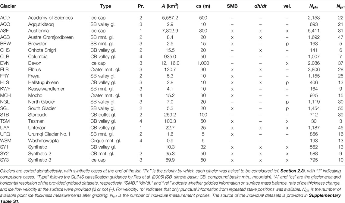
TABLE 1. Overview of the ITMIX2 test cases and data available for each glacier.

FIGURE 1

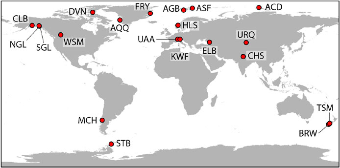
FIGURE 1. Overview of the real-world test cases considered in the frame of ITMIX2. Abbreviation keys as well as basic information for each glacier and data avialability are given in Table 1.

For every test case, glacier outlines, a digital elevation model (DEM) of the glacier surface, and a set of ice thickness observations were available. These data were retrieved from a variety of sources (see Supplementary Table S1). For 15 of the real-world cases, additional data were available for characterizing the glaciers. Depending on the case, these included information of the surface mass balance, rate of ice thickness change, or surface ice flow speed and direction. Where available, the information was provided as a gridded product, with a horizontal resolution ranging between 5 m (e.g., Washmawapta Glacier) and 1 km (Devon Ice Cap) depending on the test case. An overview of the main characteristics and of the information available for each test case is given in Table 1.

Of particular relevance for ITMIX2 were the available ice thickness observations. As is virtually always the case when acquiring such observations in the field, these data were aligned along a series of individual transects. For ITMIX2, these transects were segmented into individual profiles and numbered, giving rise to between 3 (Tasman Glacier) and 55 (South Glacier) individual profiles per test case. To ensure compatibility with the provided gridded products, and to avoid over-weighting of very densely sampled profiles in particular, the data along these profiles were spatially re-sampled. This was done by moving along the defined profiles at incremental steps of one cell size (e.g., 5 m in the case of Washmawapta Glacier, or 1 km in the case of Devon Ice Cap), and averaging any ice thickness observation within a radius of half the cell size. The averaging was performed for both the observed thickness and the observed coordinates. This procedure resulted in a thinning of the available observation, with between 30 (Tasman Glacier) and 5,411 (Austfonna Ice Cap) point observations per test case (see Table 1). The thinned profiles were at the basis of the IMTIX2 experiments described hereafter.

2.2 Experimental Design

For every ITMIX2 test case, 16 experiments were defined. In each of these experiments, the available profiles were split into two different subsets; one was made available for model calibration (“calibration profiles”), and the other was used for validation of the results (“test profiles”). The 16 experiments aimed at investigating both the effect of some peculiar layouts for the spatial distribution of the calibration profiles (experiments 01–04), as well as the effect of the amount of data available for calibration (experiments 05–16). Figure 2 visualizes the different layouts for the example of Freya Glacier.

FIGURE 2

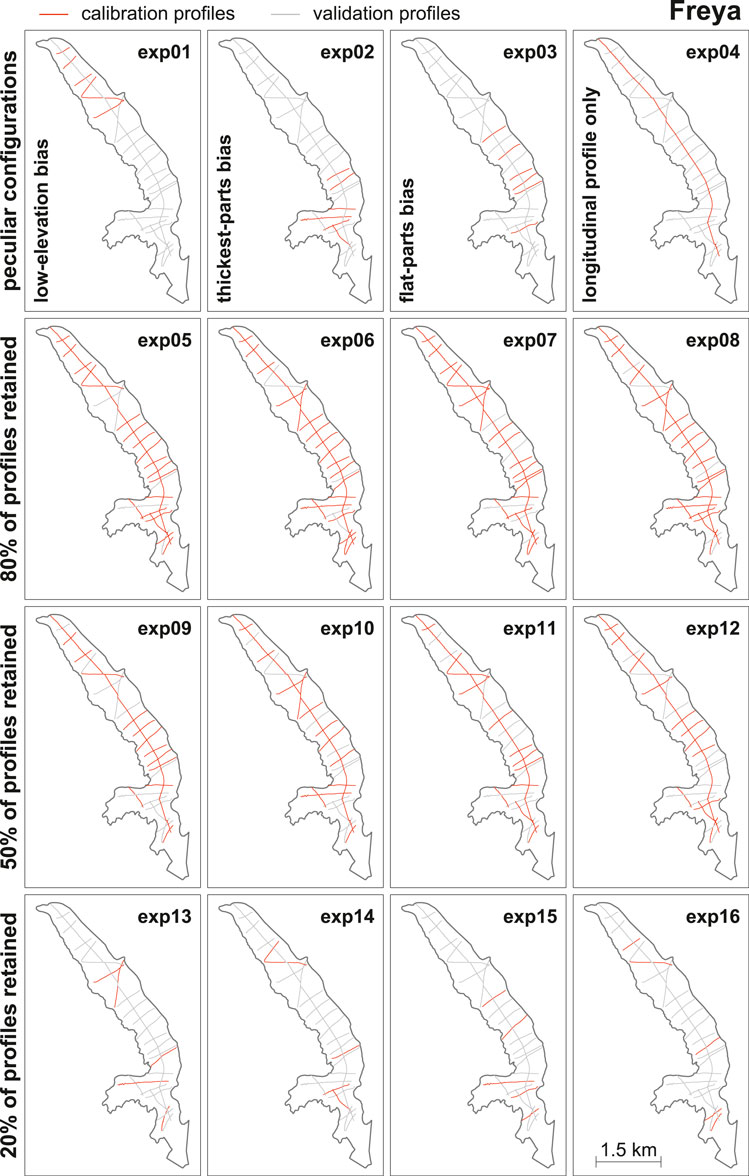
FIGURE 2. Profile layout for the 16 experiments considered within ITMIX2. Profiles indicate locations for which measured ice thickness is available. For each experiment (exp01 to exp16), a given subset of profiles was available for model calibration (red) whilst the remaining subset was used for validation (gray). Experiments 01–04 refer to peculiar configurations (see note within each panel) whilst experiments 05–16 consist of random selections of a given subset of profiles. The example refers to Freya Glacier, which is the non-compulsory test case considered by the largest number of modellers (cf. Table 2). Note the scalebar in the bottom right panel.

Experiment 01 (“low-elevation bias”) mimics the situation in which the available profiles are clustered toward the glacier’s lowermost elevations. Such a configuration is sometimes encountered for ground-based ice thickness surveys (e.g., Hagg et al., 2013; Feiger et al., 2018) when the access to higher elevations is hampered by logistics or safety constraints. For any glacier, the experiment was produced by selecting those profiles that are located in the lowest quarter of the glacier’s elevation range.

Experiment 02 (“thickest-parts bias”) represents the situation in which the available profiles preferentially capture the thickest parts of the glacier. To do so, all profiles were ranked according to the maximal ice thickness measured within each profile, and the first quarter of the profiles was chosen. The longitudinal profile was excluded to avoid producing results similar to experiment 04 (see below).

Experiment 03 (“flat-part bias”) is a configuration in which the available profiles are preferentially located in the flat parts of the glacier. Logistics and accessibility make such a situation common for ground-based ice thickness surveys. The experiment was constructed by using the available DEMs to determine the local surface slope at every measurement point of a given profile, calculating an average slope per profile, ranking the profiles with respect to this average slope, and selecting the quarter of profiles with the lowest slopes. As for experiment 02, the longitudinal profile was excluded.

Experiment 04 (“longitudinal profile only”) only provided the longitudinal profile for calibration. This configuration is sometimes encountered for airborne surveys of valley glaciers (e.g., Conway et al., 2009; Gourlet et al., 2016), when aircraft manoeuvrability prevents across-flow profiles to be acquired.

Experiments 05–08 (“80% of profiles retained”) are four different layouts in which 80% of the available profiles are retained for calibration. The four realizations are generated by randomly selecting a corresponding number of profiles. Similarly, Experiments 09–12 (“50% of profiles retained”) and 13–16 (“20% of profiles retained”) are, each, four random realizations of layouts including 50% and 20% of the available profiles, respectively.

2.3 Call for Participation and Provided Instructions

An open call for participation to ITMIX2 was posted on “cryolist” (http://cryolist.org/) on May 07, 2018. Modellers that had participated in ITMIX1 (see Section 4 in Farinotti et al., 2017) were additionally contacted on a bilateral basis and encouraged to participate. ITMIX2 instructions were provided on a dedicated web-page and data access was granted upon email-registration. Participants were asked to use the provided data to produce an estimate of the ice thickness distribution for as many test cases as possible and for each of the 16 experiments. Any approach capable of estimating glacier ice thickness from the provided input data was admitted to participation, independently of whether the approach was previously published in the literature or not.

Registered participants were provided access to all available data at once, notably including all available ice thickness measurements as well. The requirement of only using a given subset of the measurements for model calibration during the individual experiments was, thus, not controlled further but relied on the honesty of each participant.

To gauge the participants’ efforts and to ensure that a given subset of test cases would be considered by all participants, a priority was assigned to every test case (cf. Table 1). Three cases (Austfonna, Unteraar, Synthetic1) were defined as “compulsory” (priority “1”), meaning that a given approach had to provide results for at least these three cases for being considered within ITMIX2. The other test cases were assigned priorities “2” (high priority), “3” (to be considered if possible), or “4” (low priority). The three test cases with priority “1” include a mountain glacier, an ice cap, and a synthetic glacier. “Priority 4” was assigned to test cases with comparatively sparse data availability. Priorities “2” and “3” roughly follow data availability (higher priority for better data coverage) and aimed at having a mixture of test-case types (mountain glaciers, ice caps, synthetic cases). A test case was considered to be completed if results for all 16 experiments were submitted.

3 Participating Models and Submitted Results

A total of 13 models participated in the experiment, providing an ensemble of 2,544 individual solutions (159 test cases with 16 experiments each) in total (Table 2). The individual models are briefly described hereafter, whilst an overview of the submitted results is given in Section 3.2. Within the set of models, three clusters can be discerned—the clusters being defined by the similarity between individual approaches and their origin. Providing a quantitative metric for the degree of similarity between approaches would be difficult but Figure 3 visualizes the genealogy of the individual models. In principle, most models descend from the approaches presented by (1) Linsbauer et al. (2009), which applies the shallow ice approximation and an empirical relation between glacier elevation range and basal shear stress (Haeberli and Hoelzle, 1995) at the local scale, (2) Farinotti et al. (2009b), which is a flowline-based approach considering mass conservation and Glen’s ice flow law (Glen, 1955), or (3) Morlighem et al. (2011), which is based on a two-dimensional consideration of the continuity equation. The ensemble-approach GilletChaulet is of different nature, as it uses the composite result that emerged from ITMIX1 as a prior for estimating the ice thickness at locations far away from measurements (see Section 3.1.5 for details). To provide context to the performance of individual models, a trivial estimate based on the average thickness of the thickness measurements available during calibration is considered as well (Section 3.1.14).

TABLE 2

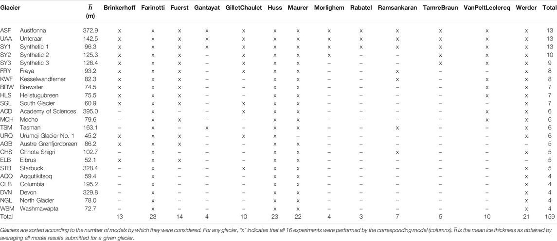
TABLE 2. Overview of the submitted model results.

FIGURE 3

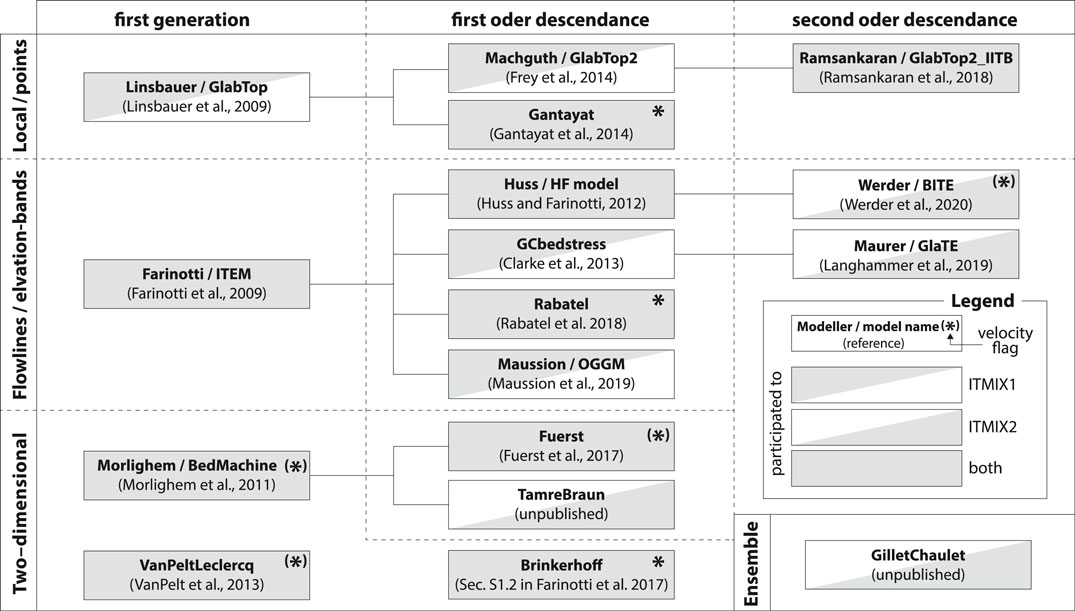
FIGURE 3. Overview of the models participating to ITMIX and their genealogy. Models are organized by their main setup (given to the left) and descendances are indicated by solid lines. The setup distinguishes between i) local, point-based methods, ii) methods that are based on ice flowlines, elevation bands, or cross-sections, and iii) methods based on two-dimensional considerations. The method GilletChaulet is a special case, as it is based on an ensemble of methods that have any of the three setups. The color of each box indicates whether a given model participated in ITMIX1, ITMIX2, or both (see legend). The “velocity flag” indicates whether an approach strictly requires ice flow velocities (asterisk) or whether it is able to use them when available (asterisk in brackets).

3.1 Description of Individual Models and Calibration Strategy

Nine of the 13 models participating to ITMIX2 already participated in ITMIX1, whilst four (the ensemble-approach GilletChaulet, and the models Maurer, TamreBraun, and Werder) joined anew. Hereafter, the models are briefly described in alphabetical order, with an emphasis on the calibration strategy chosen in the frame of ITMIX2. For further details, the reader is referred to the original publications.

3.1.1 Brinkerhoff

This model was labeled Brinkerhoff-v2 in ITMIX1 and is a further development of the approach described in Brinkerhoff et al. (2016). In brief, the approach consists of a forward model based on the Blatter-Pattyn approximation to the Stokes equations (Pattyn, 2003), and minimizes a cost-function including three terms penalizing i) differences between modeled and observed surface elevations, ii) strong spatial variations in bedrock elevations, and iii) non-zero ice thickness outside the glacier margin with respect to bedrock elevation and effective surface mass balance. As an optional additional step, a spatially-varying basal traction and/or ice hardness field is adjusted such that the misfit between modeled and observed velocity is minimized. Further details are found in Supplementary Section S1.2 of Farinotti et al. (2017).

For the different ITMIX2 experiments, calibration was performed as for ITMIX1, but with the addition of an additional term in the cost function that penalizes the misfit between modeled and observed bedrock elevation. Thus, the procedure iteratively adjusts bedrock elevation, effective mass balance, ice hardness, and basal traction such that both mass and momentum are conserved while adjusting free parameters to most closely match observations of bedrock elevation, surface elevation, and surface velocity. This minimization is performed using a simple gradient-descent procedure, with gradients computed through the adjoint method.

3.1.2 Farinotti

Sometimes referred to as Ice Thickness Estimation Method (ITEM), this model is fully described in Farinotti et al. (2009b). In it, the considered glacier is subdivided into individual ice-flow catchments, and an estimate of the ice volume flux across transects aligned along manually-defined flow lines is solved for ice thickness by using a rearranged form of Glen’s flow law (Glen, 1955). The ice volume flux is obtained by integrating the glacier’s surface mass balance distribution, which itself is derived from the glacier’s the surface topography.

For calibration, the procedure described in Farinotti et al. (2009a) was used. In a nutshell, the correction factor C (see Eq. 7 in Farinotti et al., 2009b) was adjusted to minimize the misfit between observed and modeled ice thickness at every profile with observations. The factor C accounts for a number of assumptions, including i) the linear shear stress distribution, ii) the approximation of the ice volume flux at the center of the profile with the average volume flux, and iii) the linear relation between basal sliding and surface flow speed. In any ITMIX2 experiment, C was adjusted independently for every profile available for calibration. Between profiles, the values were linearly interpolated, whilst the average value was used at the start and end of each flow line. Since C was adjusted on a profile-by-profile basis, deviations between measured and observed point thicknesses still occurred. These deviations were bi-linearly interpolated in space, and the so-obtained field of differences was subtracted from the estimated ice thickness distribution. This ensured a close match between modeled an observed thickness at every observational point.

3.1.3 Fuerst

This model was presented in Fürst et al. (2017), and consists of a two-step inverse approach solving for mass conservation. In the first step, a geometrically controlled, non-local flux solution is converted into ice thickness by relying on the shallow ice approximation (Hutter, 1983). When available, observations of ice flow velocities are then used in a second step to adjust the ice thickness distribution. To solve for mass conservation, the model uses Elmer/Ice, an open source finite element software (Gillet-Chaulet et al., 2012; Gagliardini et al., 2013).

For the individual ITMIX2 experiments, the model’s standard iterative inversion procedure was used. In the first step, ice velocities were ignored and the flux solution was directly translated into thickness values via the shallow ice approximation. In this case, the unconstrained viscosity parameter was directly calibrated to reproduce each point measurement of ice thickness. After inserting the average viscosity as inferred from all available measurements, the sparse viscosity information was linearly interpolated over the drainage basin. If 2D information on ice velocity was available, the inversion directly solved for the ice thickness field. In this second step, the resulting thickness mismatch was an additional term in the cost function that is iteratively minimized.

3.1.4 Gantayat

This model, described in Gantayat et al. (2014), relies on the equation of laminar flow (Cuffey and Paterson, 2010) and requires distributed information of the ice flow velocity at the glacier surface. A constant relation is assumed between surface ice flow velocity and basal sliding, whilst the basal shear stress is computed on the basis of surface slope (Haeberli and Hoelzle, 1995). For ITMIX2, discrete points along manually digitized branchlines were considered, and the resulting ice thickness was spatially interpolated by using the ANUDEM algorithm Hutchinson (1989) and assuming zero ice thickness at the glacier margin. The branchlines were generated requiring i) a lateral spacing of ca. 200 m between adjacent lines, ii) a minimal distance of 100 m from the glacier margin, and (iii branchlines from individual glacier tributaries gradually merging into the main tributary.

Model calibration for individual ITMIX2 experiments was performed by determining a specific shape factor f (see Eq. 2 in Gantayat et al., 2014) at the points of intersection between branchlines and profiles with ice thickness observations. For any of these points (step 1), the value of f was chosen as to minimize the difference between modeled and observed ice thickness. For branchline-points in the vicinity of available profiles (step 2), the average f-value of these profiles was assigned. For branchline-points farther apart, f was taken as the average of all values determined in the previous two steps.

3.1.5 GilletChaulet (Ensemble-Approach)

This approach differs from the other models as it relies on the results that were submitted to ITMIX1. In a nutshell, an optimal interpolation scheme is used to combine the multi-model ensemble from ITMIX1 with the observations available for calibration. Close to the observations, the measured ice thickness is returned; in the far field (i.e., ca. 10 times the maximal thickness away), the approach returns the ensemble-mean thickness of ITMIX1.

More specifically, the approach is based on the Best Linear Unbiased Estimator (BLUE) (e.g., Goldberger, 1962). Assuming a linear relation between a prior estimate ${\mathbf{h}}^b$ (referred to as to the background) and the observations ${\mathbf{h}}^o$, the BLUE estimator ${\mathbf{h}}^a$ is the one that minimises the error variances, and is given by

${\mathbf{h}}^a={\mathbf{h}}^b+\mathbf{K}\left({\mathbf{h}}^o-\mathbf{H}{\mathbf{h}}^b\right)(1)$

where $\mathbf{H}$ is the observation operator, and $\mathbf{K}$ is a function of the background error covariance matrix $\mathbf{B}$ and the observation error covariance matrix $\mathbf{R}$:

$\mathbf{K}=\mathbf{B}{\mathbf{H}}^T{\left(\mathbf{H}\mathbf{B}{\mathbf{H}}^T+\mathbf{R}\right)}^{-1}.(2)$

The assumptions are that the background and the observations are unbiased, and that both have independent errors. ${\mathbf{H}}^T$ is the matrix transpose of $\mathbf{H}$.

The individual ITMIX2 experiments were addressed by taking ${\mathbf{h}}^o$ as the set of observations available for calibration. Observation errors were assumed to be uncorrelated and to have a standard deviation of 5 m (note that no information was provided on the actual accuracy of these observations within ITMIX2). $\mathbf{H}$ was chosen to be an operator that interpolates the ice thickness from the uniform grids used in ITMIX1 to the locations of the available thickness observations. For the background, the ITMIX1 average composite solution (cf. Farinotti et al., 2017) was used, with the covariance matrix $\mathbf{B}$ being estimated from the ITMIX1 ensemble. The ITMIX1 ensemble comprises between 4 (Starbuck) and 16 (Synthetic1) individual model members, with an average of 10 members. Since covariance matrices estimated from small ensembles can exhibit spurious long-range correlations, a domain localization technique was used. This technique ensured that the thickness at a given location was updated using only observations that are within 10 times the maximum ice thickness of the background field. For locations farther apart, the ITMIX1 composite solution remains unchanged. The procedure was implemented by using the Localized Ensemble Transform Kalman Filter (Hunt et al., 2007) as provided in the Parallel Data Assimilation Framework by Nerger et al. (2005). For further details and an application of the ensemble Kalman Filter in the context of ice flow modeling, see Gillet-Chaulet (2020).

3.1.6 Huss

Sometimes referred to as HF-model, the approach was originally presented for a global-scale ice thickness reconstruction in Huss and Farinotti (2012). The model is based on the concepts of Farinotti et al. (2009b) but avoids the necessity of defining ice flow lines and catchments by performing all computations for 10 m elevation bands. Variations in the valley shape and basal shear stress along the glacier’s longitudinal profile are taken into account, as are the temperature-dependence of Glen’s flow rate factor (Glen, 1955) and the variability in basal sliding. Average elevation-band ice thickness is extrapolated on a regular grid by considering both local surface slope and distance from the glacier margin.

For ITMIX2, calibration of individual experiments was performed by a three-step procedure including (i model optimization, (ii longitudinal bias correction, and (iii spatial interpolation. First, the apparent mass balance gradient (Huss and Farinotti, 2012) was calibrated to minimize the average misfit with the available ice thickness observations. Second, the relative deviation of the modeled thickness was evaluated in 50 m elevation bands, and superimposed over the computed ice thickness distribution after smoothing. Finally, the thickness distribution was spatially interpolated based on the available thickness observations, the adjusted model results in unmeasured regions, and the condition of zero thickness on the glacier margin.

3.1.7 Maurer

This model was presented as the Glacier Thickness Estimation (GlaTE) framework in Langhammer et al. (2019a). It was specifically designed for combining the modeling results with measured ice thickness in an inversion procedure. This inversion follows the bed-stress approach by Clarke et al. (2013), which subdivides a glacier into individual ice flow sheds and uses an estimate of the glacier ice volume flux to invert for ice thickness based on Glen’s flow law. The strength of the GlaTE framework is the capability of both modularly adding further observational constraints—such as observed ice flow velocities or rates of ice thickness change for example—and accounting for observational uncertainties when available. GlaTE is open-access software and it is available at https://gitlab.com/hmaurer/glate.

The calibration procedure used for ITMIX2 followed the original approach (Langhammer et al., 2019a). In a nutshell, GlaTE sets up a system of equations comprising 1) constraints that force observed and predicted ice thickness data to match within a prescribed accuracy, 2) glaciological modeling constraints that force the ice thicknesses to comply with the model of Clarke et al. (2013), supplemented by longitudinal averaging as proposed by Kamb and Echelmeyer (1986), 3) boundary constraints that force the ice thickness to be zero outside of the glacier outlines, and 4) smoothness constraints that force the ice thickness distribution to vary smoothly. The contributions of the individual constraints can be controlled by weighting factors. Since the smoothness constraints are the least physical ones, GlaTE attempts to minimize the corresponding weighting factor. More specifically, a relatively high factor is chosen at the start and then gradually decreased until the observed and predicted thicknesses match within the prescribed error bounds. For ITMIX2, the consistency of the individual inversion runs was maximized by using the same control parameters for all experiments. This also allowed the computations to be performed in an automated fashion.

3.1.8 Morlighem

This model was originally presented in Morlighem et al. (2011) and is now also known as BedMachine (Morlighem et al., 2017; Morlighem et al., 2020). It is specifically designed to provide estimates of ice thickness between transects surveyed by radio-echo soundings, and was developed for applications over ice sheets, rather than mountain glaciers. The model is cast as an optimization problem minimizing the misfit between observed and modeled thicknesses. Being based on mass conservation, the ice thickness is computed by requiring the ice flux divergence to be balanced by the rate of thickness change and the net mass balances. When surface ice velocities were not provided, the shallow ice approximation was applied by assuming that internal deformation was about half of the total surface speed. The ice thickness was then determined by solving the resulting polynomial.

The ITMIX2 experiments were addressed by using the model’s standard framework (Morlighem et al., 2011) and did not require any specific amendment.

3.1.9 Rabatel

This model was first presented in the frame of ITMIX1, and is now fully described in Rabatel et al. (2018). In brief, the ice volume flux across individual cross-sections is quantified from information of the glacier’s surface mass balance and observed surface flow velocities. Using Glen’s flow law, this information is translated in an average ice thickness for each cross-section. This thickness is then first distributed along each cross-section by assuming a constant relation between local thickness and surface velocity, and then interpolated between cross-section by using universal Kriging with anisotropy in the main glacier flow direction. Note that the model requires information about surface ice flow speeds, thus reducing the set of test cases that can considered.

Model calibration for individual ITMIX2 experiments followed the procedure described in Rabatel et al. (2018). For each experiment, the ratio between local ice thickness h and local surface ice flow speed v is quantified for every grid cell. This ratio is then plotted against the surface elevation z, and a regression of the form $h/v=f\left(z\right)$ is performed. The type of regression (linear or polynomial) is chosen using the profiles available for calibration in order to minimize the difference between observed and modeled thickness when computing $h=v\cdot f\left(z\right)$. This inverse relation is then applied to the entire glacier by making use of the distributed information of both z (from the DEM) and v (from the maps of ice flow speed). Note that the form of the relation between h and v could be extended to include additional morphologic variables (such as surface slope or distance to the glacier margin, for example) or to be non-linear (Bolibar et al., 2020).

3.1.10 Ramsankaran

This model was labeled RAAJglabtop2 in ITMIX1, is known as GlabTop2_IITB version (Ramsankaran et al., 2018; Pandit and Ramsankaran, 2020), and is an independent re-implementation of the approach described in Frey et al. (2014). The approach itself is based on the concepts presented in Linsbauer et al. (2012) with the difference of being entirely grid-based. The local ice thickness is first calculated for a set of randomly selected grid cells, which is done from an estimate of both the basal shear stress and the surface slope. This thickness is then spatially interpolated by assigning a minimum, non-zero thickness to grid cells directly adjacent to the glacier margin.

For the individual ITMIX2 experiments, the model was calibrated by varying the dimensionless shape factor f (see Eq. 1 in Ramsankaran et al., 2018) over four levels, i.e., $f=0.6$, 0.7, 0.8, and 0.9. By doing so, f was assumed to be identical for all profiles, and the value resulting in the lowest root mean square error between modeled and observed ice thickness was chosen.

3.1.11 TamreBraun

This model has not been published so far. It is based on mass conservation, requiring ice flux divergence to be matched by mass balance and rate of ice thickness change. Ice thickness at any point on the glacier is directly computed by integration of mass balance over its catchment area. The latter is determined by repurposing the FastScape algorithm (Braun and Willett, 2013) from its use in geomorphology. Ice flow parameters in the model are optimized for the smallest misfit between modeled and observed ice thicknesses where such observations are available. A more comprehensive description of the model is found in Supplementary Section S1.

For ITMIX 2, the model parameters $f_d$ (i.e., the pre-factor for the deformation velocity) and $f_s$ (i.e., the pre-factor for the sliding velocity) were optimized to minimize the misfit ${{\displaystyle \sum }}^{\text{}}{\left(h_{\text{mod}}-h_{\text{obs}}\right)}^2$. Here, $h_{\text{mod}}$ and $h_{\text{obs}}$ are the modeled and observed ice thickness at a give location, respectively. The sum was computed over all thickness data points available in a given experiment, and the results of the run with the lowest misfit were submitted. The parameter space was explored using the neighborhood algorithm (Sambridge, 1999a; Sambridge, 1999b). Note that the algorithm is versatile enough to deal with larger parameter spaces—such as when mass balance data is not available and needs to be inferred as well—although such cases were not considered.

3.1.12 VanPeltLeclercq

This model is an adaptation of the approach by van Pelt et al. (2013), as described in Supplementary Section S1.17 of Farinotti et al. (2017). Following the concepts laid out in Leclercq et al. (2012), the model derives an ice thickness distribution by iteratively minimizing the misfit between modeled and observed elevations of the glacier surface. SIADYN—an ice dynamics model relying on the vertically integrated shallow ice approximation—is used as a forward model (SIADYN is part of the ICEDYN package; for more details, see Section 3.3 in Reerink et al., 2010) whilst basal sliding is included through a Weertman-type formulation (Huybrechts, 1991). In absence of time-dependent mass balance information, every forward model run uses a fixed surface forcing, and continues until a steady state is reached.

For the ITMIX2 experiments, an extensive 2D parameter exploration was performed. In particular, the model was set up for every test case with a varying number of iterations (that is the number of iterative steps in which the subglacial topography is adjusted) and a range of flow enhancement factors. All combinations were run, and the combination that minimized the root mean square error between observed and modeled ice thicknesses was selected. Typically, a few hundred combinations were tested before selecting the optimal ones. Within ITMIX2, 16 different combinations were chosen for every test case, depending on the configuration of the ice thickness data available for calibration within each experiment.

3.1.13 Werder

This approach was presented as the Bayesian Ice Thickness Estimation (BITE) model in Werder et al. (2020), where it is described in full detail. In brief, the approach consists of a forward model based on the approach by Huss (cf. Section 3.1.6) augmented with the capability of calculating surface flow speeds consistent with mass conservation. The mass conservation and shallow ice calculations are first conduced on elevation bands, with the resulting ice thicknesses and flow speeds being then extrapolated to the map plane. The model is fitted to ice thickness and flow speed observations (when available) using a Bayesian approach. When observational uncertainties are known, the Bayesian formulation allows for this information to be taken into account.

The individual ITMIX2 experiments were addressed by using a calibration procedure similar to the one described in Werder et al. (2020): for each experiment, the model is fitted to the available profiles with ice thickness observations and to the distributed surface flow speeds; unlike in the original procedure, however, the glacier length is not used for fitting. The error between observations and model predictions—used in the likelihood calculation—are assumed to be normally distributed with a standard deviation of 15 m for ice thickness and 30 m a⁻¹ for flow speed. Fitted model parameters include the apparent mass balance, the sliding factor, the ice temperature, and two parameters affecting the extrapolation from elevation bands to the map plane. The prior distributions of the parameters are determined by the available data or, if unavailable, by expert guesses. The fitting procedure is implemented with a Markov chain Monte Carlo method with 10⁵ steps.

3.1.14 The Simplest Model as a Benchmark

To provide context to the performance of the above models, an additional, trivial estimate of the ice thickness distribution was computed. For any test case and experiment, this estimate simply consisted of the average ice thickness of the profiles available for calibration. The estimate is assumed to be valid at any location (homogeneous thickness). We refer to this simplest possible estimate as to the benchmark, indicating that any model with a performance lower than this can be considered as virtually skill-free.

3.2 Overview of Model Submissions

The 13 models considered between 3 (compulsory only) and 23 (all) test cases (Table 2). Four models considered more than 20 cases, four models considered between 10 and 14 cases, and the remaining models considered 7 cases or less. Whilst the definition of compulsory test cases ensured that the corresponding cases were considered by all models, the definition of other categories had little effect on the choice of considered cases. Austre Grønfjordbreen, Chhota Shigri or Starbuck, for example, were all assigned priority “2” but were only considered by five models. In contrast, the “priority 3” cases Synthetic 3, Kesselwandferner, Brewster or Hellstugubreen, were all considered by seven models or more. Rather than the assigned priority, the choice seems to have been directed by data availability, with test cases with more comprehensive datasets (cf. Section 2.1) attracting or enabling more models to deliver results. It is important to note that some models strictly require information on surface ice velocity (cf. Figure 3), thus precluding the possibility of considering all test cases. In some instances, the time required for model set up was a deterrent for considering more cases (note that both ITMIX1 and ITMIX2 were community efforts run without funding and purely based on voluntary commitment). In the end, every test case was considered by at least four different models, and ten test cases were considered by more than half of the models.

4 Evaluation Procedure

4.1 Consistency Checks and Adjustments

Prior to further evaluation, the submitted results were checked for consistency and adjusted if necessary. First, any non-zero ice thickness outside of the provided glacier margins was discarded, meaning that all further evaluations refer to the area within that margins; negative or missing thicknesses within the margin (which affect roughly 1% of all submitted grid cells and arise for some models when the velocity input fields have data gaps) were set to a no-data value and were discarded from further analysis. Second, the extent and resolution of the results were adjusted as to match the originally-provided gridded data (cf. Section 2.1). Trimming of the spatial extent was necessary for some submissions of Gantayat and Fuerst, whilst a re-sampling of the resolution from 50 m grid spacing to 300 m spacing was necessary for GilletChaulet’s Austfonna results. The trimming of the extents did not require any interaction with the provided ice thickness estimates (since only the far, non-glacierized margins were affected), whilst the re-sampling in the case of Austfonna was performed by computing averages of the 36 cells with 50 m resolution contained within each 300-m cell. The cause of these discrepancies can be traced back to the affected models using the topography-data distributed within ITMIX1, rather than ITMIX2. We stress that both the trimming and the re-sampling do not alter the ice thickness estimates, and note that the no-data values introduced through the first adjustment step only potentially affect the results when they concern grid-cells that are intersected by measurement profiles (i.e., <<1% of all cells).

4.2 Evaluation of Model Performance

In all analyses that follow, the model performance for any given experiment is evaluated against those ice thickness observations that were not available for calibration during that particular experiment. Deviations are always expressed as “model minus observation,” negative values thus indicating that a given model underestimates the ice thickness.

Since no consistent information on the accuracy of the ice thickness observations was available for the combination of data-sources used within ITMIX2 (Supplementary Table S1), the observations are all considered to be error-free for the calculations that follow. Whilst average deviations over multiple points remain unaffected as long as stochastic errors are assumed, we acknowledge that error-free observations are not realistic. We also note that the assumption of stochastic errors might hold over the ensemble of all measurements, but might be questionable for individual glaciers. This is because the observations of a given test case often stem from an individual field campaign, and systematic interpretation errors are thus difficult to exclude.

To enable direct comparison between modeled thicknesses (which are gridded) and observed thicknesses (which refer to multiple profiles and can be available at any location), the observed thicknesses are first rasterized on the modeling grid. For every grid-cell, this is done by computing the arithmetic average of all observations that fall within that cell. To allow for comparability between test cases of different size and thickness, deviations are further expressed as percent-deviations from the mean ice thickness of the corresponding test case. Since the “true” mean ice thickness is unknown, it is computed by averaging all model results submitted for a given test case; that is, the average thickness is the result of averaging over all models, all experiments, and all grid-cells of that particular case (the resulting values are given in Table 2). This evaluation strategy follows the one used during ITMIX1, and ensures that average percent-deviations are not skewed by large relative deviations that may occur when local thickness is small. For a hypothetical glacier that is 50 m thick on average, for example, overestimating the thickness of a 1 m-thick marginal grid-cell by say, 10 m, results in a deviation of $+20$%, and not $+\mathrm{1,000}$% as if point-thickness were considered.

5 Results and Discussion

5.1 Characteristics of Results Submitted by Individual Models

The results submitted by individual models can be characterized by three indicators: 1) the standard deviation ${\sigma }_{\text{n}}$ between individual solutions at profiles that were not used for calibration (“test profiles”), 2) the deviation $\text{Δ}{h}_{\text{n}}$ between modeled and observed ice thickness at the test profiles, and 3) the deviation $\text{Δ}{h}_{\text{c}}$ between modeled and observed ice thickness for profiles that were available for calibration.

The first indicator, σ_n, quantifies the degree to which similar solutions are produced when different calibration data are provided. High values suggest that a given model is very sensitive to these data, with very different results being provided depending on which subset of profiles was used for calibration. Extremely low values, instead, indicate that the calibration procedure is insensitive to the input. Moderate values might thus be preferential as they hint at a compromise between model robustness and sensitivity. To compute σ_n for a given location, we determine the difference between modeled h_m and observed h_o ice thickness for all experiments during which that point was part of the test profiles (that is a set of up to 16 values), divide by the mean ice thickness $\overline{h}$ of the considered glacier, and compute the standard deviation of the so-obtained differences (that is one value per location): ${\sigma }_n=\text{stdev}\left(\left(h_m-h_o\right)/\overline{h}\right)$. Figure 4A shows the distribution of σ_n when the quantity is pooled across all test cases and is stratified by model. Large values of ${\sigma }_{\text{n}}$ are found for the models Morlighem and Farinotti, which show median σ_n values of $\sim$30% the mean ice thickness. For comparison, the benchmark model shows a median σ_n of 17.2%. Low values, instead, are found for Brinkerhoff, Gantayat, the ensemble-approach GilletChaulet, Rabatel, VanPeltLeclerq and Werder, which all have σ_n medians below 13%. A remarkable exception is the model Ramsankaran, for which the median σ_n is close to zero. This means that the model provides the same solution independently of the profiles used for model calibration, and indicates that the chosen calibration procedure (cf. Section 3.1.9) tended to select the same shape factor for all experiments. We note that this could be resolved by following a calibration procedure such as the one adopted in Ramsankaran et al. (2018), who defined a variable shape factor depending on elevation and other topographical properties.

FIGURE 4

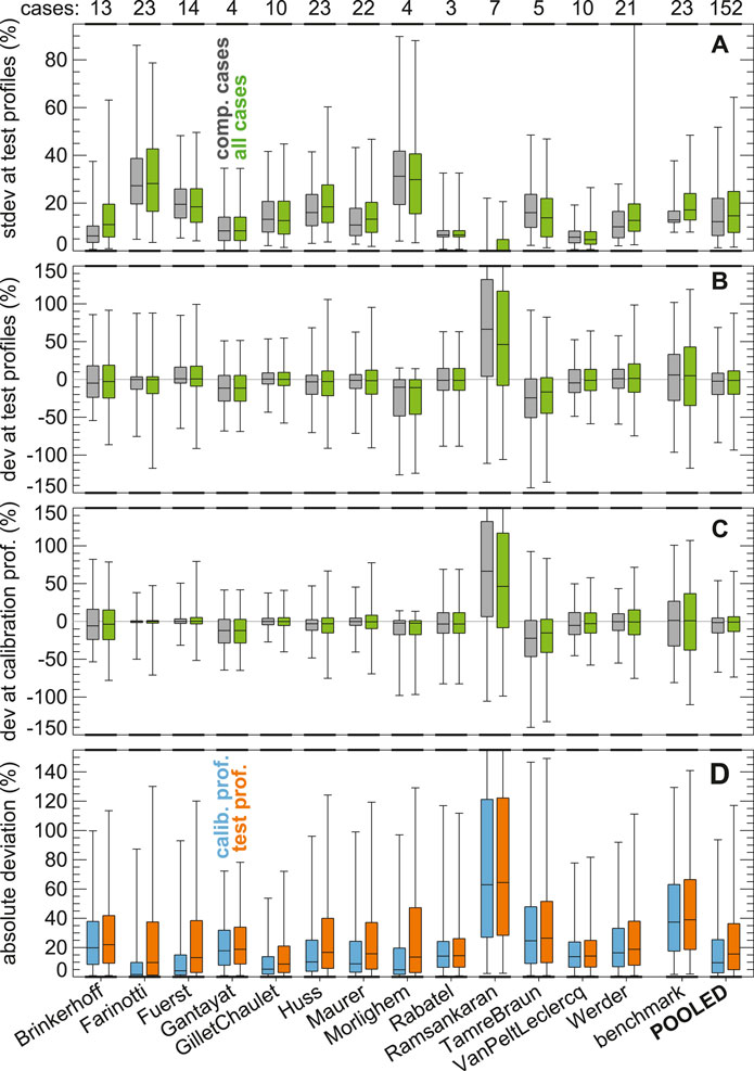
FIGURE 4. Overview characteristics for the results provided by each model. (A) Standard deviation (stdev) of the difference between modeled and observed ice thickness at the locations of profiles that were not used for model calibration (here referred to as “test profiles”). The number of test cases considered by each model is given above the panel. (B) Deviations (dev) between modeled and observed ice thickness at the same locations. (C) Same as (B) but for profiles that were available during model calibration. (D) Absolute deviations for all test cases. In (A–C), gray and green boxplots refer to the compulsory test cases and all test cases, respectively (see Table 1). In (D), blue and orange boxplots refer to test and calibration profiles, respectively. The set of boxplots labeled with “POOLED” combine the deviations across models but excludes the results of both the Ramsankaran-model (due to the large bias) and the benchmark. Boxplots show the 95% confidence interval (whiskers), the interquartile range (box), and the median (lines within box). All values are expressed relatively to the mean ice thickness of the corresponding glacier.

The above model behavior is confirmed by the indicator $\text{Δ}{h}_{\text{c}}$, i.e., by the deviation of the modeled ice thickness at the calibration profiles (again, the quantity is first computed individually for every location and model, and then pooled across test cases and experiments). Whilst most models show a distribution of $\text{Δ}{h}_{\text{c}}$ centered around zero (Figure 4C), Ramsankaran shows median deviations in the order of +50%, thus indicating a systematic overestimation of the actual thickness. Slight biases are also found for Gantayat and TamreBraun, with median $\text{Δ}{h}_{\text{c}}$ in the order of $-15$%. The distribution of $\text{Δ}{h}_{\text{c}}$ also reveals that some models aim at matching the calibration data exactly (e.g., Farinotti, Fuerst, the ensemble-approach GilletChaulet and Maurer have interquartile ranges below 10%) whilst other approaches allow the modeled thickness to fluctuate around the measured thickness (the interquartile range for Brinkerhoff, TamreBraun and VanPeltLeclerq, for example, is in the order of 30–40%). The latter is the expression of a compromise between agreement with observations—which can be affected by unknown uncertainties and biases—and internal model consistency—which is governed by the conservation of mass and/or momentum in the mentioned models. Again for comparison, the benchmark model shows an interquartile range of 60% whilst it is unbiased ($\text{Δ}{h}_{\text{c}}\approx$ 0%) by design.

The indicator $\text{Δ}{h}_{\text{n}}$, finally, quantifies the models’ capabilities of correctly predicting the ice thickness at unmeasured locations. The distribution of $\text{Δ}{h}_{\text{n}}$ is shown in Figure 4B, and reveals that whilst the median deviations remain virtually unaltered and centered around zero in most cases, the difference between modeled and observed thickness increases significantly when compared to locations with thickness observations (cf. indicator $\text{Δ}{h}_{\text{c}}$). The first observation can be interpreted as a confirmation that the implemented calibration procedures are unbiased (pooled across models but excluding the results by Ramsankaran, the median deviation is $-2.3$% and $-1.3$% of the mean ice thickness for the compulsory and all cases, respectively). The second observation is expected, and is expressed in a change of the interquartile ranges and confidence intervals, for example. On average over the 13 considered models, the two quantities increase by 10% and 30% of the mean ice thickness, respectively. Of particular notice are the models that displayed a bias in $\text{Δ}{h}_{\text{c}}$. In those cases, the distribution of $\text{Δ}{h}_{\text{n}}$ is skewed. Such skewness is particularly prominent in the model Ramsankaran (biased toward an overestimation of the thickness) and, to a lesser degree, Morlighem and TamreBraun.

The increased difference between modeled and observed thickness when comparing the deviations for the test profiles against the calibration profiles, is also noticeable in a general shift of the absolute values of the deviations toward higher values (Figure 4D). Of notice is that the shift is minor for several models ($<$1.5% for Gantayat, Rabatel, Ramsankaran, and VanPeltLeclercq, for instance), indicating that these models provide similar results independently of the spatial distribution of the calibration profiles (in line with the indicator σ_n). The results also show that, apart from Ramsankaran, the median deviation to point measurements is within 16% of the mean ice thickness on average, and within 31% of the mean thickness for three-quarters of the cases. Particularly good performances are found for the ensemble-approach GilletChaulet and the models Rabatel and VanPeltLeclercq, where three quarters of the point deviations remain within 26.1% of the mean ice thickness. The benchmark model shows median deviations of 38.9% and three quarters of the deviations contained within 66.4%.

An example for how the characteristics discussed above express themselves in the actual ice thickness distribution is given in Figure 5: two profiles are shown for the compulsory test case Unteraar and the ensemble-approach GilletChaulet (featuring medium σ_n, and small $\text{Δ}{h}_{\text{c}}$ and $\text{Δ}{h}_{\text{n}}$), as well as the models Morlighem (large σ_n, skewed $\text{Δ}{h}_{\text{c}}$ and $\text{Δ}{h}_{\text{n}}$), and VanPeltLeclerq (small σ_n, medium $\text{Δ}{h}_{\text{c}}$ and $\text{Δ}{h}_{\text{n}}$). An equivalent representation comprising all models is given in Supplementary Figures S1, S2, whilst examples for other test cases are found in Supplementary Figures S3–S6 and the digital materials (see URL in the Data Availability Statement).

FIGURE 5

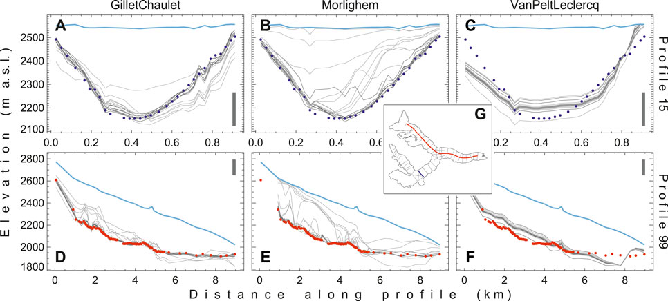
FIGURE 5. Examples of the results provided by individual models. (A–F) Results of individual experiments (gray lines), shown for two selected profiles of the compulsory test case “Unteraar.” Experiments in which the given profile was available for calibration (dark gray lines) are distinguished from those in which the profile was not available (light gray). The location of the profiles is given in the map inset (G). The glacier surface (solid blue line) and direct ice thickness observations [blue and red dots for the (A–C) across-glacier and (D–F) along-glacier profile, respectively] are shown. The ensemble-approach GilletChaulet illustrates a case with medium spread between solutions of different experiments (i.e., medium σ_n), and a relatively close match between modeled and observed ice thickness at both profiles used and not used during model calibration (i.e., small $\text{Δ}{h}_{\text{c}}$ and small $\text{Δ}{h}_{\text{n}}$). Morlighem is a case in which σ_n is large, and both $\text{Δ}{h}_{\text{c}}$ and $\text{Δ}{h}_{\text{n}}$ are skewed toward low ice thicknesses. VanPeltLeclercq displays small σ_n, and medium $\text{Δ}{h}_{\text{c}}$ and $\text{Δ}{h}_{\text{n}}$. The thick, dark gray vertical bar to the left of each panel visualizes the mean glacier thickness. The results of all models are shown in Supplementary Figures S1, S2. Examples profiles for the other compulsory cases are shown in Supplementary Figures S3–S6. An equivalent representation for all test cases and all profiles (499 figures in total) is provided at the URL given in the Data Availability Statement.

Of further notice in Figures 4A–C is that the characteristics of individual models remains very similar if only compulsory test cases are considered (cf. gray and green boxplots for models that considered more than three cases). The results and Figures of the next sections thus refer to all submissions of each model, and do not further discern the compulsory cases separately. Figures that only consider the compulsory test cases are given in Supplementary Figures S7–S9.

5.2 Influence of the Availability of Ice Thickness Observations

Since ice thickness observations are generally sparse, an important question is how the performance of individual models reacts to the amount of ice thickness data available for calibration. Figure 6A shows how the absolute deviation between modeled and observed ice thickness evolves for experiments 05 to 16, i.e., during the experiments in which the availability of calibration profiles is reduced.

FIGURE 6

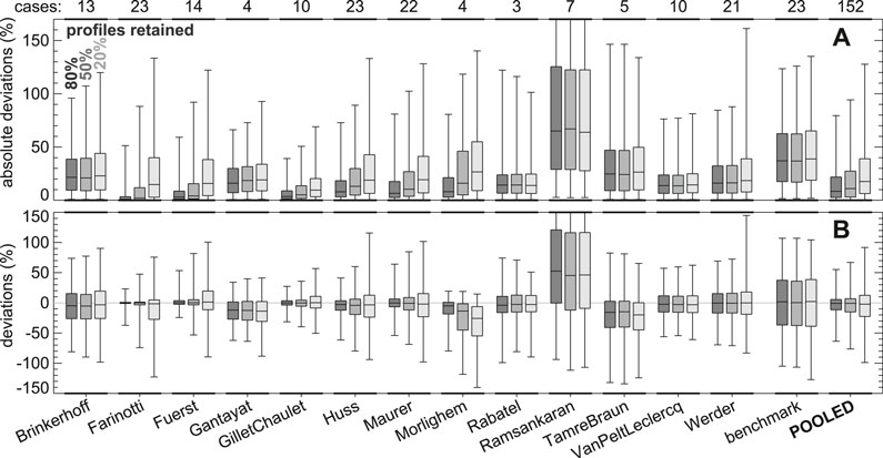
FIGURE 6. Distributions of model deviations when only a given subset of ice thickness observations is provided for calibration. The color of the boxplots indicates the share of profiles retained during calibration, with experiments retaining the same share being pooled across test cases. i.e., for every model, dark boxplots pool the results of all glaciers for experiments 05 to 08, in which 80% of the available profiles were retained for model calibration; medium and light boxplots refer to the cases in which 50% (experiments 09–12) and 20% (experiments 13–16) of the profiles were retained, respectively. Values are given relatively to the mean glacier thickness. “POOLED” boxplots combine the deviations across models but exclude both Ramsankaran and benchmark. Boxplots are defined in Figure 4. Panel (A) is the same as (B) but refers to the absolute values of the deviations. The number of test cases considered by each model is given above panel A. The equivalent representation for the case in which only compulsory test cases are considered is given in Supplementary Figure S7.

As expected, the deviations increase when fewer observations are available. Pooled across models and excluding both the benchmark and the visibly biased Ramsankaran, the results show that the median absolute deviations increase from 8.4% of the mean ice thickness when 80% of the measured profiles are retained for calibration (experiments 05–08), to 11.0% when 50% of the profiles are retained (experiments 09–12), and to 17.6% when only 20% are retained (experiments 13–16). Three quarters of the deviations are within 21.8%, 27.4%, and 39.0% of the mean ice thickness when 80%, 50%, and 20% of the profiles are retained, respectively. For the benchmark model, the median deviations remain unaltered at about 38% for all three experimental sets (three quarters of the deviations within 45%), indicating that the four random realizations within each set were sufficient for avoiding any bias (such a bias would be conceivable if one realization had preferentially sampled profiles with, say, shallower thicknesses).

A set of three models (Farinotti, Fuerst, and the ensemble-approach GilletChaulet) displays very good agreement with the ice thickness observations not used for calibration when 80% of the profiles are retained (80%-retained experiments from now on), with median deviations within 3.5% the mean thickness and with three quarters of the deviations below 9%. Together with Huss, Maurer, and Morlighem, however, these models also show a relatively pronounced decrease in performance when fewer data are available. On average over the six models, for example, the average level below which three quarters of the deviations are contained rises from 13.0% of the mean ice thickness for the 80%-retained experiments to 39.3% for the 20%-retained experiments. This is in contrast to other models, which display less sensitivity to the availability of observations. The standard deviation of the same metric across the 80%-retained, 50%-retained, and 20%-retained experiments, for instance, is below 4% the mean ice thickness for all of Brinkerhoff, Gantayat, Rabatel, TamreBraun, VanPeltLeclerq, and Werder (note, however, that Werder displays a substantial increase in outliers when reducing the data availability from 50% of profiles retained to 20%; in these two cases, the 95% confidence interval increases from 87.8% the mean ice thickness to 161.3%).

The interpretation of the different behaviors between the two model clusters is not straightforward. Indeed, the consistency between various experiments could be both an indication for model stability (i.e., the models’ capability of extracting information from limited subsets of ice thickness observations) or an indication for the models’ calibration strategy not being able to take various profile configurations fully into account. A hint for this latter interpretation might be seen in the fact that the more stable models display consistently larger deviations than the other models in the 80%-retained experiments. In these cases and on average, the models Brinkerhoff, Gantayat, Rabatel, TamreBraun, VanPeltLeclerq, Werder show a median absolute deviation of 17.7% the mean ice thickness, whilst the same metric is as low as 5.0% for Farinotti, Fuerst, Huss, Maurer, Morlighem, and the ensemble-approach GilletChaulet. We note again that approaches emphasizing internal model consistency might face difficulties in accommodating all provided observational constraints, i.e., might have difficulties in finding an estimate that is not only consistent with the provided ice thickness observations but is also compatible with the available surface mass balances, rates of ice thickness change, and ice flow velocity fields (cf. Table 1). Missing consistency could be the result either of a model that does not correctly capture the physics of the glacier, or of a bias in one or several of the input datasets.

For individual models, the response to a decrease in ice thickness observations available for calibration is difficult to interpret when considering larger outliers. For Rabatel and TamreBraun in particular, the 95% confidence interval of the deviations between modeled and observed ice thickness decreases when comparing the 50%-retained experiments to the 20%-retained ones. The decrease is of $-$14.9% and $-$12.6% for the two models, respectively. Whilst the result might be spurious since the models only considered a limited subset of test cases (three and five, respectively; cf. Table 2), this observation might need to be further investigated.

An important observation emerges when considering actual deviations (Figure 6B), rather than their absolute values. Indeed, the distribution of these deviations confirms the unbiasedness of the model ensemble, particularly showing that the average deviation does not drift toward more positive or more negative values as data availability decreases. Pooled across models (and again excluding Ramsankaran and the benchmark), for example, the median deviation remains within 2.1% of the mean ice thickness in all cases, and fluctuates by less than 1.3% when passing from the 80%-retained experiments to the 20%-retained ones. On the one hand, this observation confirms the results of ITMIX1, in which the advantages of using a model ensemble rather than an individual model was shown. On the other hand, it shall be noted that the observation of no drift also holds true when considering the models individually. This indicates that even a limited subset of ice thickness observations is effective in constraining the mean ice thickness and glacier volume predicted by individual models. An exception is given by Morlighem, where the 20%-retained experiments show a lowering of the predicted thickness by about 21% when compared to the 80%-retained experiments. This seems to indicate that the method is more strongly influenced by the condition of zero ice thickness at the glacier margin than other models are, and could be addressed by lowering the regularization term used to enforce smoothness in the computed thickness fields.

A further quantitative indication for how the availability of ice thickness observations typically influences model accuracy, can be obtained by investigating the dependence between the model accuracy at the point scale and the distance to the closest ice thickness observation available during model calibration (Figure 7). Pooled across all models and all experiments, this relation indicates that the accuracy decays almost linearly with the logarithm of the distance to the next observation. The median absolute deviation is 7.7%, 15.7%, 21.4%, and 33.2% of the mean ice thickness when the closest observation is at a distance of 0.1, 1, 10, and 100 times the mean ice thickness, respectively (on average, results change by less than 2.5% when only compulsory test cases are considered although deviations as high as 5.6% occur for the largest distances considered). The relation is specific to every model (Supplementary Figure S3), with the differences between them echoing the characteristics highlighted above. Some models, for example, show a less prominent decrease in accuracy with increasing distance to the available observations, hinting at their capability of extracting information of thickness measurements further apart. Models that have a particularly slow increase in deviations with distance include Gantayat, Rabatel, VanPeltLeclercq, Werder, and the ensemble-approach GilletChaulet.

FIGURE 7

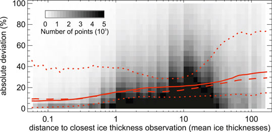
FIGURE 7. Difference between modeled and observed ice thickness as a function of the closest ice thickness observation available for model calibration. Both the difference and the distance are expressed in relation to the mean ice thickness. The figure is based on a total of ca. 1.8 million points, obtained by pooling all models, all test cases, and all experiments. The shading in the background provides the number of points falling within each area of the plot. The solid (dashed) red line is a fit through the median deviation at each given distance when all (only compulsory) test cases are considered. The dotted lines are an envelope containing the equivalent fits of all individual models, apart from Ramsankaran and benchmark. The results for the individual models are shown in Supplementary Figure S8.

5.3 Influence of the Distribution of Ice Thickness Observations

The effect that the spatial distribution of the ice thickness observations has on the model performance is quantified through experiments 01 to 04. Figure 8A shows the absolute deviation between modeled and observed ice thickness at profile locations not used during calibration.

FIGURE 8

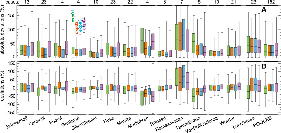
FIGURE 8. Distributions of model deviations when the ice thickness observations provided for calibration show a peculiar spatial distribution. The colors of the individual boxplots discern the situations in which the observations are biased toward low elevations (exp01), the thickest parts (exp02), or the flattest parts (exp03) of the glacier. In exp04, only observations along a longitudinal profile are provided (cf. Figure 2). Values are given relatively to the mean glacier thickness. “POOLED” boxplots combine the deviations across models and exclude Ramsankaran and benchmark. Boxplots are defined in Figure 4. Panel (A) (number of test cases considered by each model given above the panel) is the same as (B) but refers to the absolute values of the deviations. The equivalent representation for the case in which only compulsory test cases are considered is given in Supplementary Figure S9.

Pooled across models (again excluding Ramsankaran and benchmark), the experimental configurations mimicking a low-elevation bias (exp01) and providing a longitudinal profile only (exp04) show somewhat higher deviations than the situations in which the available observations are biased toward the thickest (exp02) and flattest (exp03) part of the glaciers. Averaged over the first two cases (exp01 and 04), three quarters of the deviations are contained within 50.7% of the mean ice thickness, whilst the same metric decreases to 44.5% on average over experiments 02 and 03.

The effect is particularly visible for Morlighem, Fuerst, and Farinotti, where the median absolute deviation for experiments 01 and 04 is 32.7%, 15.5%, and 13.3% higher than on average for experiments 02 and 03, respectively (percentages refer to the mean ice thickness). The same pattern is visible to a lesser degree in TamreBraun and Huss, with changes of 11.5% and 10.0%, respectively. The concomitant changes in the experiments with a bias in observations toward the thickest and flattest parts of the glacier can be explained by these two conditions often corresponding, i.e., by the fact that the flat glacier parts often coincide with the thickest. With this in mind, it is not unexpected that the model results are generally closer to the observations when thickness information is available for the thickest parts of a glacier: constraining the modeling results on these locations provides less room for very large deviations to occur, which is particularly beneficial when aiming at characterizing the total glacier volume.

Despite the above, it shall again be noted that the bias introduced by the individual measurement configurations is small (Figure 8B). Brinkerhoff, Farinotti, Huss, Maurer, VanPeltLeclerq, Werder, and the ensemble-approach GilletChaulet, show particular robustness against the individual configurations, with the median actual deviations of the four experiments showing a standard deviation below 4.7% of the mean ice thickness. At most, these models show a slight tendency for an increase in outliers when only a longitudinal profile is available for calibration. Note that the term “actual deviations” is used here to distinguish these deviations from the absolute values discussed above. The combination of small actual deviations with large absolute deviations indicates that a model correctly capture the mean ice thickness but that it does so by overestimating the thickness in some areas and underestimating it in some other.

The only systematic deviations emerge for the situation in which the observations are preferentially available for low elevations. In such cases, several models underestimate the actual ice thickness (and even the consistent overestimation by Ramsankaran seems slightly reduced), with the most prominent biases shown by Morlighem (median deviation corresponding to $-61.5$% of the mean ice thickness), TamreBraun ($-52.6$%), and Gantayat ($-22.0$%). The bias can be explained by i) the lowermost elevations of glaciers often also being the thinnest, and ii) the fact that various modeling approaches implicitly assume the considered glaciers to be in steady state. The first explanation is supported by the results of the benchmark model, which shows a bias of $-22.4$% for the particular configuration. The assumption of a steady state, instead, is clearly unsuitable for most present-day glaciers, which show substantial thinning rates especially at low elevations. For approaches based on mass or momentum conservation, this causes the ice flux to be underestimated, resulting in an ice thickness that is too thin throughout the glacier. Together, the result indicates that—although if convenient from the logistical point of view—survey configurations in which low elevations are sampled preferentially should be avoided, or at least complemented with measurements selectively gathered on thicker glacier parts.

5.4 Combined Model Performance

The results of the previous sections leave open the question whether a single best model, or a subset of best performing models, can be discerned. We tackle this question by defining a relative score that combines the results shown in Figures 4, 6, 8: for any of the boxplots within these figures, we use the i) median, ii) interquartile range, and iii) 95% confidence interval as separate indicators, and assign a given score. If $\mathbf{X}=\left[X_1,X_2,\dots ,X_n\right]$ is a set of n indicator values (for example the set 15 medians of the boxplots referring to the compulsory cases in Figure 4A) with absolute values $\mathbf{Y}=\left|\mathbf{X}\right|$, then the set of scores $\mathbf{S}$ is given by

$\mathbf{S}=\frac{\mathbf{Y}-\text{min}\left(\mathbf{Y}\right)}{\text{max}\left(\mathbf{Y}\right)-\text{min}\left(\mathbf{Y}\right)}.(3)$

The score thus assumes a value of $S_i=1$ for the best performing model i (in the example, the model with smallest median), and of $S_j=0$ for the worst performing model j (the model with the largest median). The overall model score is then defined to be the average score for all 66 considered indicators (22 boxplots with three indicators each). Due to the large biases discussed earlier, the model Ramsankaran is not ranked.

The results of the above scoring procedure are shown in Figure 9, which differentiates between the case in which all test cases (Figure 9A) or only compulsory test cases (Figure 9B) are considered. The only model that consequently stands out is the ensemble-approach GilletChaulet: in the score, the model stands at least 0.11 points above any of the other models. The other models are all within 0.28 score points, apart from Morlighem, TamreBraun, and benchmark. This indicates that the bulk of the models have comparable performance and that, unfortunately, it is difficult to provide a recommendation in favor of one or the other approach, particularly given that the uncertainty in the various data products used to drive individual models is not robustly quantified. Similar is true when attempting to group the models with respect to, e.g., the “descendance” shown in Figure 3 or the type of input data used by the individual models. Indeed, no systematic picture emerges, with members of different groups scattered across the ranking (Figure 9).

FIGURE 9

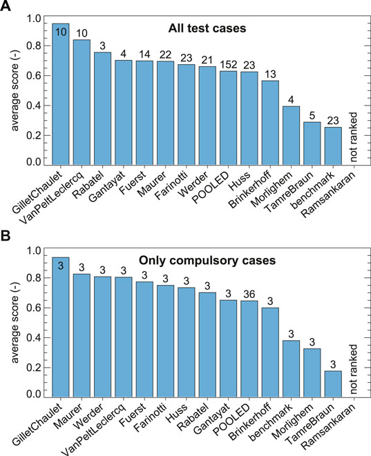
FIGURE 9. Average score of model performance in the case that (A) all or (B) only compulsory test cases are considered. The number of test cases considered by each model is given above the bars. The score is based on the medians, interquartile ranges and 95% confidence intervals shown in Figures 4, 6, 8 (66 indicators in total). A score of “1” (“0”) would indicate that the corresponding model performs best (worst) in all of the 66 indicators. The model Ramsankaran is not ranked for the reasons discussed in the text. “POOLED” refers to the pool of models besides Ramsankaran and benchmark.

We acknowledge that the relatively small number of test cases available within ITMIX2, as well as the different number of test cases considered by the different models, somewhat limit the possibility of more robust statements in the above respect. The sensitivity to these points becomes apparent, for example, when comparing the ranking obtained for all experiments (Figure 9A) with that obtained by only considering compulsory test cases (Figure 9B): in the first case, VanPeltLeclercq and Rabatel obtain above-average scores whilst in the second, Maurer and Werder score better than VanPeltLeclercq, and Rabatel ranges mid-way. A similar change in position is observable for Gantayat, whilst Farinotti, Huss, and Brinkerhoff seem more stable in their ranking positions.

6 Summary and Conclusions

ITMIX2 was the second phase of the Ice Thickness Models Intercomparison eXperiment. Aiming at characterizing the degree to which models inferring the ice thickness distribution from characteristics of the glacier surface can benefit from sparse in-situ thickness observations, it attracted the participation of 13 different modeling approaches. A set of 23 test cases including both real-world and synthetically generated glaciers and ice caps was considered, and 16 different experiments were conducted to infer the effect that both availability and spatial distribution of ice thickness observations have on model performance. The main results of ITMIX2 can be summarized as follows:

• The characteristics of the participating models are highly variable (Figures 4A,B). Whilst some models provide similar results independently of the amount and spatial distribution of ice thickness observations available for calibration, other models show typical variabilities in the results of different experiments in the order of 30% the mean ice thickness. Whilst low variabilities are an indication for model robustness in most instances, they seem to reflect a lack of flexibility in the calibration procedure in individual cases. It is reassuring that all but one approach consistently outperformed a simple benchmark model based on the average thickness at observed locations.

• Even for locations at which ice thickness observations exist, the strategy for taking these into account varies between models (Figures 4C,D, 5). Whilst some models aim at ensuring a close match between observed and modeled ice thickness, some others favor the internal model consistency prescribed by the continuity equation. For the latter set of models, the deviations at locations with ice thickness observations available during model calibration can show interquartile ranges as high as 30–40% the mean ice thickness.

• For most models, a few observations are sufficient to correctly capture the mean glacier thickness (Figure 6). This follows from the observation that the bias of individual models does not drift during the experiments in which the amount of ice thickness observations available for model calibration is artificially reduced. This is particularly reassuring for applications that depend on estimates of the glaciers’ total volume, rather than the complete ice thickness distribution. Still, median deviations of around 16% the mean ice thickness are typical for locations that are not covered by measurements, and one quarter of the deviations even exceed 37% of the mean ice thickness (Figure 4D).

• In general, the accuracy of local ice thickness estimates decreases with the availability of ice thickness observations (Figure 6) and with the distance to the next observation in particular (Figure 7). On average over all models and all experiments, the median deviation between model results and observations increases by 8.5% the mean ice thickness when the distance to the next observation is increased by a factor of 10. That is: the median difference is about 8% when the closest observation is within one 10th of the mean ice thickness, about 16% when it is one mean thickness away, and about 21% when it is at a distance equivalent to ten times the mean ice thicknesses. The latter value is close to the $\pm$24% average deviation found in the frame of ITMIX1, where no measured ice thickness was provided at all, thus providing an indication for the typical distance at which the information-content of the measurements is no longer useful to inform the models. It must be noted, however, that the relation is specific to each model, and can vary significantly between the models (Supplementary Figure S7).

• With the exception of a few models, the spatial distribution of the ice thickness observations has only a weak effect on the modeled thickness distribution (Figure 8). The only configuration to be avoided is the one in which observations preferentially sample the lowest elevations of a glacier. Although convenient from the logistical point of view, this configuration can over-sample thin glacier parts thus resulting in a bias toward underestimated ice thickness. On the contrary, a preferential sampling of the thickest glacier parts prevents large deviations, successfully constraining the total glacier volume.

• The applicability of individual models is highly variable. Whilst some models are readily applicable also to larger sets of glaciers and even when input data are constrained to a minimum, other models strictly require additional information, such as distributed ice flow velocities of the glacier surface (Figure 3), or require a considerable time investment for model setup. The latter two points limit the applicability of some models to small sets of glaciers. A special case is given by the ensemble-approach of GilletChaulet: the necessity of having a prior-estimate based on the results of several models, clearly increases the workload of its application.

In light of the above, a recommendation for a single best model cannot be made. On the one hand, the models by Farinotti and Fuerst as well as the ensemble-approach GilletChaulet are noticeable as they ensure a close match of the available thickness observations (Figures 4C). On the other hand, the combination of performed experiments and considered metrics (Figures 4, 6, 8, 9, as well as Supplementary Figures S7, S9) suggest that the models Brinkerhoff, Farinotti, Fuerst, Gantayat, Huss, Maurer, Rabatel, VanPeltLeclercq, and Werder all have similar performance, with Maurer, Werder, and VanPeltLeclercq showing above-average performance when only compulsory test cases are considered, and VanPeltLeclercq and Rabatel showing above-average performance when considering all test cases (note that in this latter case, models that considered only few cases, such as Rabatel for instance, are somewhat advantaged). Only the ensemble-approach GilletChaulet consistently stands out for its enhanced robustness toward varying configurations of available observational thickness—including configurations in which data availability is particularly limited. ITMIX2 thus confirms the result of the first phase of the intercomparison experiment (Farinotti et al., 2017), which already pointed at the added value of using a model ensemble instead of an individual approach.

ITMIX2 also highlights the limitations that the present generation of models still have in predicting the ice thickness distribution of individual glaciers. Whilst it shows that even sparse sets of ice thickness observations are effective in preventing model biases, it also cautions against the relatively large uncertainties that can exist at the local scale. The latter are often linked to the uncertainties that affect observational data other than ice thickness, such as the elevation of the glacier surface, the ice velocity, the surface mass balance or the rate of ice thickness change. Indeed, models that include such auxiliary information face the need of prioritizing the matching of one or another dataset. For this to happen in a meaningful way, information about the accuracy of the individual datasets, as well as model capabilities to cope with observational uncertainty, are essential.

The considerations above highlight the value and importance of ongoing initiatives aiming at mapping the ice thickness and other essential glaciological parameters at the global scale. Together with ongoing efforts of centralizing and making publicly available the corresponding observations, such endeavors will help in both the continued development of the necessary models, and the better characterization of the ice reserves locked in today’s ice masses.

Data Availability Statement

The i) datasets originally distributed to the participating modellers, ii) results submitted by every modeller, iii) data shown in the main figures, as well as iv) an extended set of figures are found at https://doi.org/10.3929/ethz-b-000447116. The source code for the ensemble-approach GilletChaulet is available at https://gricad-gitlab.univ-grenoble-alpes.fr/gilletcf/itmix2https://www.frontiersin.org/articles/10.3389/feart.2020.571923.

Author Contributions

DF designed the study, with input from JF, MH, LA and other participants of ITMIX phase one. DF, DB, JF, PG, FG, MH, PL, HM, MM, AP, AR, RR, TR, ElR, EmR, ET, WvP, and MW performed the modeling with individual approaches. MA and AP provided data for Chotta Shigri Glacier. With inputs from all co-authors, DF evaluated the results, wrote the manuscript, and designed and produced all figures and tables.

Funding

JF was financed by the German Research Foundation (DFG) within the Svalbard-iFLOWbed project, Grant FU1032/1-1. AR and FG acknowledge the support of LabEx OSUG@2020 (Investissements d’avenir—ANR10 LABX56). MW was partly funded by the ESA project Glaciers_cci (4000109873/14/I-NB).

Conflict of Interest

Author AP was employed by the company Tata Consultancy Services (TCS).

The remaining authors declare that the research was conducted in the absence of any commercial or financial relationships that could be construed as a potential conflict of interest.

The reviewer (DS) declared a past co-authorship with one of the authors (MM) to the handling editor.

Acknowledgments

The work is a contribution of the Working Group of Ice Thickness Estimation, which acted under the umbrella of the International Association of Cryospheric Sciences. We are thankful to all researchers that contributed to the dataset of ITMIX phase one (http://dx.doi.org/10.5905/ethz-1007-92), as well as to Ivan Lavrentiev, Geir Moholdt, and Thomas Schuler for the additional data provided for Austre Groenfjordbreen, and to Etienne Berthier for providing the DEM of Chhota Shigri. Results provided by JF are based on numerical simulations conducted at the high-performance computing center of the Regionales Rechenzentrum Erlangen (RRZE) of the University of Erlangen-Nuremberg.

Supplementary Material

The Supplementary Material for this article can be found online at: https://www.frontiersin.org/articles/10.3389/feart.2020.571923/full#supplementary-material.

References

Bamber, J. L., Baldwin, D. J., and Gogineni, S. P. (2003). A new bedrock and surface elevation dataset for modelling the Greenland ice sheet. Ann. Glaciol. 37, 351–356. doi:10.3189/172756403781815456

CrossRef Full Text | Google Scholar

Bamber, J. L., Griggs, J. A., Hurkmans, R. T. W. L., Dowdeswell, J. A., Gogineni, S. P., Howat, I., et al. (2013). A new bed elevation dataset for Greenland. The Cryosphere 7, 499–510. doi:10.5194/tc-7-499-2013

CrossRef Full Text | Google Scholar

Blindow, N., Salat, C., and Casassa, G. (2012). “Airborne GPR sounding of deep temperate glaciers—examples from the northern Patagonian Icefield,” in 14th international conference on ground penetrating radar (GPR), Shanghai, China, (Piscataway, NJ: Institute of Electrical and Electronics Engineers (IEEE)), 664–669. doi:10.1109/ICGPR.2012.6254945

CrossRef Full Text | Google Scholar

Bolibar, J., Rabatel, A., Gouttevin, I., Galiez, C., Condom, T., and Sauquet, E. (2020). Deep learning applied to glacier evolution modelling. The Cryosphere 14, 565–584. doi:10.5194/tc-14-565-2020

CrossRef Full Text | Google Scholar

Braun, J., and Willett, S. D. (2013). A very efficient O(n), implicit and parallel method to solve the stream power equation governing fluvial incision and landscape evolution. Geomorphology 180-181, 170–179. doi:10.1016/j.geomorph.2012.10.008

CrossRef Full Text | Google Scholar

Brinkerhoff, D. J., Aschwanden, A., and Truffer, M. (2016). Bayesian inference of subglacial topography using mass conservation. Front. Earth Sci. 4, 1–15. doi:10.3389/feart.2016.00008

CrossRef Full Text | Google Scholar

Clarke, G. K. C., Anslow, F. S., Jarosch, A. H., Radić, V., Menounos, B., Bolch, T., et al. (2013). Ice volume and subglacial topography for western Canadian glaciers from mass balance fields, thinning rates, and a bed stress model. J. Clim. 26, 4282–4303. doi:10.1175/JCLI-D-12-00513.1

CrossRef Full Text | Google Scholar

Conway, H., Smith, B., Vaswani, P., Matsuoka, K., Rignot, E., and Claus, P. (2009). A low-frequency ice-penetrating radar system adapted for use from an airplane: test results from Bering and Malaspina Glaciers, Alaska, USA. Ann. Glaciol. 50, 93–97. doi:10.3189/172756409789097487

CrossRef Full Text | Google Scholar

Cuffey, K., and Paterson, W. (2010). The physics of glaciers. 4th edn. Oxford, United Kingdom: Elsevier.

Google Scholar

Farinotti, D., Brinkerhoff, D. J., Clarke, G. K. C., Fürst, J. J., Frey, H., Gantayat, P., et al. (2017). How accurate are estimates of glacier ice thickness? Results from ITMIX, the Ice Thickness Models Intercomparison eXperiment. Cryosphere 11, 949–970. doi:10.5194/tc-11-949-2017

CrossRef Full Text | Google Scholar

Farinotti, D., Huss, M., Bauder, A., and Funk, M. (2009a). An estimate of the glacier ice volume in the Swiss Alps. Global Planet. Change 68, 225–231. doi:10.1016/j.gloplacha.2009.05.004

CrossRef Full Text | Google Scholar

Farinotti, D., Huss, M., Bauder, A., Funk, M., and Truffer, M. (2009b). A method to estimate the ice volume and ice-thickness distribution of alpine glaciers. J. Glaciol. 55, 422–430. doi:10.3189/002214309788816759

CrossRef Full Text | Google Scholar

Farinotti, D., Huss, M., Fürst, J. J., Landmann, J., Machguth, H., Maussion, F., et al. (2019). A consensus estimate for the ice thickness distribution of all glaciers on Earth. Nat. Geosci. 12, 168–173. doi:10.1038/s41561-019-0300-3

CrossRef Full Text | Google Scholar

Feiger, N., Huss, M., Leinss, S., Sold, L., and Farinotti, D. (2018). The bedrock topography of Gries- and Findelengletscher. Geogr. Helv. 73, 1–9. doi:10.5194/gh-73-1-2018

CrossRef Full Text | Google Scholar

Fretwell, P., Pritchard, H. D., Vaughan, D. G., Bamber, J. L., Barrand, N. E., Bell, R., et al. (2013). Bedmap2: improved ice bed, surface and thickness datasets for Antarctica. Cryosphere 7, 375–393. doi:10.5194/tc-7-375-2013

CrossRef Full Text | Google Scholar

Frey, H., Machguth, H., Huss, M., Huggel, C., Bajracharya, S., Bolch, T., et al. (2014). Estimating the volume of glaciers in the Himalayan-Karakoram region using different methods. Cryosphere 8, 2313–2333. doi:10.5194/tc-8-2313-2014

CrossRef Full Text | Google Scholar

Fürst, J. J., Gillet-Chaulet, F., Benham, T. J., Dowdeswell, J. A., Grabiec, M., Navarro, F., et al. (2017). Application of a two-step approach for mapping ice thickness to various glacier types on Svalbard. Cryosphere 11, 2003–2032. doi:10.5194/tc-11-2003-2017

CrossRef Full Text | Google Scholar

Gagliardini, O., Zwinger, T., Gillet-Chaulet, F., Durand, G., Favier, L., de Fleurian, B., et al. (2013). Capabilities and performance of Elmer/Ice, a new-generation ice sheet model. Geosci. Model Dev. 6, 1299–1318. doi:10.5194/gmd-6-1299-2013

CrossRef Full Text | Google Scholar

Gantayat, P., Kulkarni, A. V., and Srinivasan, J. (2014). Estimation of ice thickness using surface velocities and slope: case study at Gangotri Glacier, India. J. Glaciol. 60, 277–282. doi:10.3189/2014JoG13J078

CrossRef Full Text | Google Scholar

Gärtner-Roer, I., Naegeli, K., Huss, M., Knecht, T., Machguth, H., and Zemp, M. (2014). A database of worldwide glacier thickness observations. Global Planet. Change 122, 330–344. doi:10.1016/j.gloplacha.2014.09.003

CrossRef Full Text | Google Scholar

Gillet-Chaulet, F. (2020). Assimilation of surface observations in a transient marine ice sheet model using an ensemble Kalman filter. Cryosphere 14, 811–832. doi:10.5194/tc-14-811-2020

CrossRef Full Text | Google Scholar

Gillet-Chaulet, F., Gagliardini, O., Seddik, H., Nodet, M., Durand, G., Ritz, C., et al. (2012). Greenland ice sheet contribution to sea-level rise from a new-generation ice-sheet model. Cryosphere 6, 1561–1576. doi:10.5194/tc-6-1561-2012

CrossRef Full Text | Google Scholar

Glen, J. W. (1955). The creep of polycrystalline ice. Proc. R. Soc. Lond. Ser. A 228, 519–538. doi:10.1098/rspa.1955.0066

CrossRef Full Text | Google Scholar

Goldberger, A. S. (1962). Best linear unbiased prediction in the generalized linear regression model. J. Am. Stat. Assoc. 57, 369–375. doi:10.1080/01621459.1962.10480665

CrossRef Full Text | Google Scholar

Gourlet, P., Rignot, E., Rivera, A., and Casassa, G. (2016). Ice thickness of the northern half of the Patagonia Icefields of South America from high‐resolution airborne gravity surveys. Geophys. Res. Lett. 43, 241–249. doi:10.1002/2015GL066728

CrossRef Full Text | Google Scholar

Haeberli, W., and Hoelzle, M. (1995). Application of inventory data for estimating characteristics of and regional climate-change effects on mountain glaciers: a pilot study with the European Alps. Ann. Glaciol. 21, 206–212. doi:10.3198/1995AoG21-1-206-21210.1017/s0260305500015834

CrossRef Full Text | Google Scholar

Hagg, W., Mayer, C., Lambrecht, A., Kriegel, D., and Azizov, E. (2013). Glacier changes in the Big Naryn basin, Central Tian Shan. Global Planet. Change 110, 40–50. doi:10.1016/j.gloplacha.2012.07.010

CrossRef Full Text | Google Scholar

Hunt, B. R., Kostelich, E. J., and Szunyogh, I. (2007). Efficient data assimilation for spatiotemporal chaos: a local ensemble transform Kalman filter. Physica D: Nonlinear Phenom. 230, 112–126. doi:10.1016/j.physd.2006.11.008

CrossRef Full Text | Google Scholar

Huss, M., and Farinotti, D. (2012). Distributed ice thickness and volume of all glaciers around the globe. J. Geophys. Res. 117, 24–28. doi:10.1029/2012JF002523

CrossRef Full Text | Google Scholar

Hutchinson, M. F. (1989). A new procedure for gridding elevation and stream line data with automatic removal of spurious pits. J. Hydrol. 106, 211–232. doi:10.1016/0022-1694(89)90073-5

CrossRef Full Text | Google Scholar

Hutter, K. (1983). Theoretical glaciology; material science of ice and the mechanics of glaciers and ice sheets. Tokyo: Terra Scientific Publishing Company.

Google Scholar

Huybrechts, P. (1991). The Antartic ice sheet and enviremental change: a three-dimensional modelling study. PhD thesis. Brussel: Vrije Universiteit of Brussel. doi:10013/epic.12054.d001

CrossRef Full Text | Google Scholar

Kamb, B., and Echelmeyer, K. A. (1986). Stress-gradient coupling in glacier flow: I. longitudinal averaging of the influence of ice thickness and surface slope. J. Glaciol. 32, 267–284doi:10.3189/s0022143000015604

CrossRef Full Text | Google Scholar

Langhammer, L., Grab, M., Bauder, A., and Maurer, H. (2019a). Glacier thickness estimations of alpine glaciers using data and modeling constraints. Cryosphere 13, 2189–2202. doi:10.5194/tc-13-2189-2019

CrossRef Full Text | Google Scholar

Langhammer, L., Rabenstein, L., Schmid, L., Bauder, A., Grab, M., Schaer, P., et al. (2019b). Glacier bed surveying with helicopter-borne dual-polarization ground-penetrating radar. J. Glaciol. 65, 123–135. doi:10.1017/jog.2018.99

CrossRef Full Text | Google Scholar

Leclercq, P. W., Pitte, P., Giesen, R. H., Masiokas, M. H., and Oerlemans, J. (2012). Modelling and climatic interpretation of the length fluctuations of Glaciar Frías (north Patagonian Andes, Argentina) 1639-2009 AD. Clim. Past 8, 1385–1402. doi:10.5194/cp-8-1385-2012

CrossRef Full Text | Google Scholar

Linsbauer, A., Paul, F., and Haeberli, W. (2012). Modeling glacier thickness distribution and bed topography over entire mountain ranges with GlabTop: application of a fast and robust approach. J. Geophys. Res. 117, 17–19. doi:10.1029/2011JF002313

CrossRef Full Text | Google Scholar

Linsbauer, A., Paul, F., Hoelzle, M., Frey, H., and Haeberli, W. (2009). “The Swiss Alps without glaciers—a GIS-based modelling approach for reconstruction of glacier beds,” in Proceedings of geomorphometry 2009, Zurich, 243–247. Available atwww.geomorphometry.org/Linsbauer2009.

Google Scholar

Lythe, M. B., and Vaughan, D. G., and The BEDMAP Consortium (2001). BEDMAP: A new ice thickness and subglacial topographic model of Antarctica. J. Geophys. Res. 106, 11335–11351. doi:10.1029/2000JB900449

CrossRef Full Text | Google Scholar

Morlighem, M., Rignot, E., Binder, T., Blankenship, D., Drews, R., Eagles, G., et al. (2020). Deep glacial troughs and stabilizing ridges unveiled beneath the margins of the Antarctic ice sheet. Nat. Geosci. 13, 132–137. doi:10.1038/s41561-019-0510-8

CrossRef Full Text | Google Scholar

Morlighem, M., Rignot, E., Seroussi, H., Larour, E., Ben Dhia, H., and Aubry, D. (2011). A mass conservation approach for mapping glacier ice thickness. Geophys. Res. Lett. 38, 27–32. doi:10.1029/2011GL048659

CrossRef Full Text | Google Scholar

Morlighem, M., Williams, C. N., Rignot, E., An, L., Arndt, J. E., Bamber, J. L., et al. (2017). BedMachine v3: complete bed topography and ocean bathymetry mapping of Greenland from multibeam echo sounding combined with mass conservation. Geophys. Res. Lett. 44, 11051–11061. doi:10.1002/2017GL074954

CrossRef Full Text | Google Scholar

Nerger, L., Hiller, W., and Schröter, J. (2005). “PDAF-the parallel data assimilation framework: experiences with Kalman filtering,” in Use of high performance computing in meteorology. (London, UK: World Scientific). 63–83. doi:10.1142/9789812701831_0006

CrossRef Full Text | Google Scholar

Pandit, A., and Ramsankaran, R. (2020). Modeling ice thickness distribution and storage volume of glaciers in Chandra Basin, western Himalayas. J. Mt. Sci. 17,2011–2022. doi:1doi:10.1007/s11629-019-5718-y

CrossRef Full Text | Google Scholar

Pattyn, F. (2003). A new three-dimensional higher-order thermomechanical ice sheet model: basic sensitivity, ice stream development, and ice flow across subglacial lakes. J. Geophys. Res. 108, 2382. doi:10.1029/2002JB002329

CrossRef Full Text | Google Scholar

Plewes, L. A., and Hubbard, B. (2001). A review of the use of radio-echo sounding in glaciology. Prog. Phys. Geogr. Earth Environ. 25, 203–236. doi:10.1177/030913330102500203

CrossRef Full Text | Google Scholar

Pritchard, H. D., King, E. C., Goodger, D. J., McCarthy, M., Mayer, C., and Kayastha, R. 2020). Towards Bedmap Himalayas: development of an airborne ice-sounding radar for glacier thickness surveys in High-Mountain Asia. Ann. Glaciol. 61, 35–45. doi:10.1017/aog.2020.29

CrossRef Full Text | Google Scholar

IPCC (2020). IPCC special report on the ocean and cryosphere in a changing climate. Editors H.-O. Pörtner, D. C. Roberts, V. Masson-Delmotte, P. Zhai, M. Tignor, E. Poloczanskaet al. (Cambridge, United Kingdom: Cambridge University Press).

Google Scholar

Rabatel, A., Sanchez, O., Vincent, C., and Six, D. (2018). Estimation of glacier thickness from surface mass balance and ice flow velocities: a case study on Argentière Glacier, France. Front. Earth Sci. 6, 112. doi:10.3389/feart.2018.00112

CrossRef Full Text | Google Scholar

Ramsankaran, R., Pandit, A., and Azam, M. F. (2018). Spatially distributed ice-thickness modelling for Chhota Shigri glacier in western Himalayas, India. Int. J. Remote Sens. 39, 3320–3343. doi:10.1080/01431161.2018.1441563

CrossRef Full Text | Google Scholar

Rau, F., Mauz, F., Vogt, S., Khalsa, S. J. S., and Raup, B. (2005). Illustrated GLIMS glacier classification manual. Boulder, United States: Institut für Physische Geographie Freiburg, Germany, and National Snow and Ice Data Center. Version 1.0.

Google Scholar

Reerink, T. J., Kliphuis, M. A., and van de Wal, R. S. W. (2010). Mapping technique of climate fields between GCM’s and ice models. Geosci. Model Dev. 3, 13–41. doi:10.5194/gmd-3-13-2010

CrossRef Full Text | Google Scholar

RGI Consortium (2017). Randolph Glacier Inventory—a dataset of global glacier outlines: Version 6.0. Global land ice measurements from space (GLIMS). Colorado, United States: Digital Media. doi:10.7265/N5-RGI-60

CrossRef Full Text | Google Scholar

Rutishauser, A., Maurer, H., and Bauder, A. (2016). Helicopter-borne ground-penetrating radar investigations on temperate alpine glaciers: a comparison of different systems and their abilities for bedrock mapping. Geophysics 81, WA119. doi:10.1190/geo2015-0144.1

CrossRef Full Text | Google Scholar

Sambridge, M. (1999a). Geophysical inversion with a neighbourhood algorithm—I. Searching a parameter space. Geophys. J. Int. 138, 479–494. doi:10.1046/j.1365-246X.1999.00876.x

CrossRef Full Text | Google Scholar

Sambridge, M. (1999b). Geophysical inversion with a neighbourhood algorithm—II. Appraising the ensemble. Geophys. J. Int. 138, 727–746. doi:10.1046/j.1365-246x.1999.00900.x

CrossRef Full Text | Google Scholar

Schroeder, D. M., Bingham, R. G., Blankenship, D. D., Christianson, K., Eisen, O., Flowers, G. E., et al. (2020). Five decades of radioglaciology. Ann. Glaciol. 61, 1–13doi:10.1017/aog.2020.11

CrossRef Full Text | Google Scholar

van Pelt, W. J. J., Oerlemans, J., Reijmer, C. H., Pettersson, R., Pohjola, V. A., Isaksson, E., et al. (2013). An iterative inverse method to estimate basal topography and initialize ice flow models. Cryosphere 7, 987–1006. doi:10.5194/tc-7-987-2013

CrossRef Full Text | Google Scholar

Welty, E., Zemp, M., Navarro, F., Huss, M., Fürst, J. J., Gärtner-Roer, I., et al. (2020). Worldwide version-controlled database of glacier thickness observations. Earth Syst. Sci. Data 2020, 1–27. doi:10.5194/essd-2020-87

CrossRef Full Text | Google Scholar

Werder, M. A., Huss, M., Paul, F., Dehecq, A., and Farinotti, D. 2020). A Bayesian ice thickness estimation model for large-scale applications. J. Glaciol. 66, 137–152. doi:10.1017/jog.2019.93

CrossRef Full Text | Google Scholar

Zamora, R., Uribe, J., Oberreuter, J., and Rivera, A. (2017). “Ice thickness surveys of the southern patagonian ice field using a low frequency ice penetrating radar system,” in First IEEE international symposium of geoscience and remote sensing (GRSS-Chile), Valdivia, Chile, June 15–16, 2017, 1–4. doi:10.1109/GRSS-CHILE.2017.7996003

CrossRef Full Text | Google Scholar