Application of Time Series Analysis to Estimate Drawdown From Multiple Well Fields

1 Introduction

The competition for groundwater resources is fierce, including demands for agricultural production, drinking water supply, groundwater-dependent ecosystems, and for mitigation of land subsidence to maintain the stability of buildings. Dry summers and the growing demand for freshwater increases the pressure on limited groundwater resources. The groundwater table may drop significantly during and after dry summers (e.g., Brakkee et al., 2022) due to a set of stresses on the system including a decrease in precipitation, an increase in evaporation and transpiration, lower surface water levels, and higher groundwater use for both drinking water and irrigation (e.g., Van Loon et al., 2016). The effect of pumping wells on the head is one of the few stresses on the system that can be controlled. Estimates of the head response to pumping wells are therefore salient information for decision makers to manage groundwater resources and possibly mitigate low groundwater tables.

The effect of pumping on the heads in a multi-aquifer system can be estimated with a numerical groundwater model (e.g., Anderson et al., 2015). Such process-based models typically require a large amount of input data to incorporate system and process details (e.g., Hugman and Doherty, 2022). Significant time investment is required to build and calibrate these models, and, even after considerable effort, they are rarely able to simulate the transient head variation with reasonable accuracy. Alternatively, models based on time series analysis are generally much better at simulating the heads measured in an observation well (e.g., Bakker and Schaars, 2019). Additionally, time series models have the advantage of low data requirements and can be developed in a short amount of time.

Many time series analysis approaches are black-box models, for example ARIMA models (e.g., Patle et al., 2015) or deep learning methods (e.g., Wunsch et al., 2018). A disadvantage of such black-box models is that it can be difficult to physically interpret the resulting models. More transparent, gray-box approaches include lumped conceptual models (Mackay et al., 2014) or time series modeling using physically-based response functions (e.g., Von Asmuth et al., 2012; Collenteur et al., 2019). The latter also allows for the differentiation between the stresses causing the head variation (e.g., Von Asmuth et al., 2008).

An important application of time series analysis is the estimation of the drawdown caused by pumping. For example, Von Asmuth et al. (2008), Obergfell et al. (2013), and Shapoori et al. (2015) applied time series analysis to determine the drawdown due to pumping from a single well field. Many observation wells worldwide are impacted by multiple well fields. The pumping rates at these well fields are commonly correlated, which complicates the estimation of the contributions of different well fields and may lead to increased uncertainty in the model outcomes and less robust models.

The objective of this paper is to present a data-driven, reproducible, and robust approach to estimate the head response at observation wells that are potentially affected by variations in rainfall, evaporation, rivers stages, and pumping from multiple well fields. The main objective is to quantify both the magnitude and timing of the head response to the surrounding well fields at each observation well using a new parsimonious approach to incorporate multiple well fields in a time series model. The approach is tested in an area of the Netherlands where the heads are measured at 213 observation wells at multiple depths, resulting in 395 head time series. The heads are potentially affected by four different well fields. A detailed decision tree is developed to determine which stresses have a significant effect on the head variation. Time series analysis is conducted with the open-source Pastas software (version 0.20.0 Collenteur et al., 2019) to determine the response of each well field. The analysis is entirely implemented in Python scripts and is fully reproducible as advocated by Fienen and Bakker (2016) & White et al. (2020).

In the following, the approach to quantify the effects of groundwater pumping using time series analysis is presented. Next, the study area and all available data are described and the results of the analysis are presented including an estimate of the uncertainty. A possible application of the results is presented for the mitigation of low heads in dry summers. The applicability and limitations of the method are discussed, including some challenges faced while performing the study. Concluding remarks are presented at the end of this paper.

2 Methodology

A time series model represents an independent estimate of the contribution of different stresses on the heads in an observation well that is derived exclusively from observed data. A multi-model approach is applied to determine which hydrological stresses are relevant in describing the head dynamics in an observation well.

Precipitation-excess, river stage, and groundwater pumping are included as potentially relevant hydrological stresses. Eight different model structures are tested for each head time series. The simplest model considers only precipitation-excess, computed from precipitation and potential evaporation. The next model adds the river stage as a stress. In the next three models, up to three well fields are added as potential stresses, starting from the closest well field and moving towards the farthest one. The final three models repeat this last step but leave out the river as a stress.

A set of criteria is used to determine which model structures are deemed reliable. The best model structure is selected from the set of reliable models for each observation well. Split-sample testing, in which a portion of the time series is kept separate, is applied to test the calibrated model.

2.1 Time Series Modeling

The time series modeling approach, also referred to as transfer function noise modeling, uses physically-based impulse response functions that describe the head response to different stresses (Von Asmuth et al., 2002). Simulation of the effect of precipitation-excess, river stage variations, and noise modeling is based on the standard approach of Von Asmuth et al. (2008). The time series model is written as

$h\left(t\right)=\sum _{m=1}^M{h}_m\left(t\right)+d+r\left(t\right)(1)$

where h(t) are the observed heads, h_m(t) is the contribution of stress m to the head, d is the base elevation of the model, and r(t) are the residuals. Each model has an arbitrary number of stresses M, depending on the chosen model structure. The contribution of each stress is computed through convolution as

$h_m\left(t\right)={\int }_{-\infty }^t{S}_m\left(\tau \right){\theta }_m\left(t-\tau \right)d\tau (2)$

where S_m(t) is the time series of a stress m and θ_m is the associated impulse response function. An auto-regressive noise model of order 1 (AR1) is used in an attempt to transform the residuals into a noise time series n(t) that is approximately white noise (Von Asmuth and Bierkens, 2005)

$n\left(t_i\right)=r\left(t_i\right)-{\text{e}}^{\left(t_i-t_{i-1}\right)/\alpha }(3)$

where n(t_i) is the remaining noise at time t_i and α is the auto-regressive parameter.

The precipitation-excess, N(t), is modeled as

$N\left(t\right)=P\left(t\right)-f{E}_r\left(t\right)(4)$

where P(t) is the precipitation, E_r(t) is the Makkink reference evaporation (de Bruin and Lablans, 1998), and parameter f is used to scale the reference evaporation to local hydrological conditions. The impulse response of groundwater to precipitation-excess is described using the scaled Gamma distribution (Collenteur et al., 2019)

$\theta \left(t\right)=\frac{A}{a^n\mathrm{\Gamma }\left(n\right)t^{1-n}}{\text{e}}^{-t/a}(5)$

where A, a, and n are fitting parameters. In this formulation of the response function, parameter A is the gain of the response function, i.e., the rise in the head due to a constant unit precipitation-excess. The groundwater response to river stage fluctuations is described with an exponential response function, which is a special case of the scaled Gamma response function with n = 1.

The head response to groundwater pumping may be simulated with a response function that has the same mathematical form as the Hantush well function (Hantush and Jacob, 1955). There is a risk of over-parameterization of a time series model when multiple pumping wells are added to the model that each have their own response function and corresponding parameters. For example, adding three pumping wells with a Hantush well function would already add 9 parameters to the model. The use of a single response function is proposed, scaled with the distance to the well field, to quantify the effect of all groundwater pumping wells. The response function is based on the Hantush response function used by Von Asmuth et al. (2008) and is modified to include the distance of the well field to the observation well r explicitly, so that the impulse response function is

$\theta \left(r,t\right)=\frac{A}{2t}{\text{e}}^{-t/a-ab{r}^2/t}(6)$

where A, a, and b are fitting parameters. The gain of the response function is $A{\text{K}}_0(2r\sqrt{b})$, where K₀ is the modified Bessel function of the second kind and order zero. It is noted here that the parameter A for this response function does not equal the gain.

The step response Θ(t), the response to a constant unit stress, is obtained from the impulse response function through integration

$\mathrm{\Theta }\left(t\right)={\int }_0^t\theta \left(t-\tau \right)\text{d}\tau (7)$

An example of the Hantush step response is shown in Figure 1. The t₅₀ and t₉₅ represent the time when 50 and 95% of the total response has occurred, respectively. For this modified Hantush response function, the t₅₀ can be conveniently computed following Veling and Maas (2010).

$t_{50}=ar\sqrt{b}(8)$

FIGURE 1

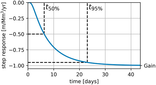
FIGURE 1. An example of the Hantush step response. The t₅₀ and t₉₅ represent the time when 50 and 95% of the total response has occurred, respectively.

The calculation of the variances of the gain and the t₅₀ is provided in the Supplementary Material.

2.2 Model Calibration, Reliability Criteria, and Selection

The most complex model considered in this paper has a total of eleven parameters: four parameters for the response to precipitation-excess, two parameters for the response to river stages, three parameters for the response to pumping wells, one parameter for the noise model, and one parameter for the base elevation of the model.

The head time series of each observation well is divided into a calibration period and a validation period. The calibration data is used to calibrate each time series model with a two-step optimization approach following Collenteur et al. (2021). In the first step, the parameters are optimized without the use of a noise model by minimizing the sum of squared residuals. In the second step, the noise model is added and the sum of squared noise is minimized using the optimized model parameters from the first step as initial parameter values.

A set of criteria is applied to all eight model structures to determine which model structures are considered reliable for further analysis. A reliable model is defined here as a model meeting four acceptance criteria. From the model structures passing these criteria, a single model structure is selected for each observation well based on two selection criteria. The selection scheme including all reliability criteria is presented in Figure 2. The following four acceptance criteria are used:

1) Goodness of fit. The model goodness of fit in the calibration period, measured as the coefficient of determination (R²), must be equal or larger than 0.7, which means that the model has at least a basic fit.

2) Autocorrelation. There must be no significant autocorrelation in the noise. This is determined with the Runs-test for autocorrelation (Wald and Wolfowitz, 1940) using a significance level of α = 0.05. This requirement is important to obtain reliable estimates of the parameter uncertainties (Hipel and McLeod, 1994).

3) Response time. The response time, expressed as the t₉₅ (see Figure 1), must not exceed half the length calibration period. The calibration time series is potentially too short to accurately estimate the parameters of the response function when the t₉₅ of the response is longer than half the length of the calibration period.

4) Uncertainty of gain. The estimated gain of each response function must be significantly different from zero. This is checked by requiring that the estimated gain is larger than twice the estimated standard deviation of the gain (e.g., Collenteur et al., 2019).

FIGURE 2

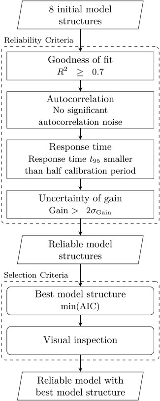
FIGURE 2. Criteria for reliable models and selection of best model structure.

When multiple model structures are reliable, the Akaike Information Criterion (AIC; Akaike, 1974) is used to select the best model structure, by selecting the model with the lowest AIC (Burnham et al., 2011). After the AIC selection, the selected model structure is visually inspected for both the calibration and validation periods. Model structure must perform well in both the calibration and the validation period.

The described approach to determine the best model structure for each observation well is applied to all observation wells in a study area. The entire analysis is implemented in Python scripts to ensure reproducibility of the results. All data, scripts, and environment settings required to reproduce the results from this study are available from Zenodo (Brakenhoff et al., 2022).

3 Study Site and Data

The study area is the Overbetuwe area in the Netherlands, a polder region of approximately 30 km by 10 km, flanked by two branches of the Rhine river (see Figure 3). The land surface elevation varies from around +10 m in the east to around +7 m in the west (all elevations are given relative to the Dutch reference level called NAP, which is approximately equal to mean sea-level). The region is divided into several polders that each strive to keep water levels at a fixed level with a complex system of ditches, canals, weirs, and pumping stations. The land use is a mix of agriculture, nature, and urban environments.

FIGURE 3

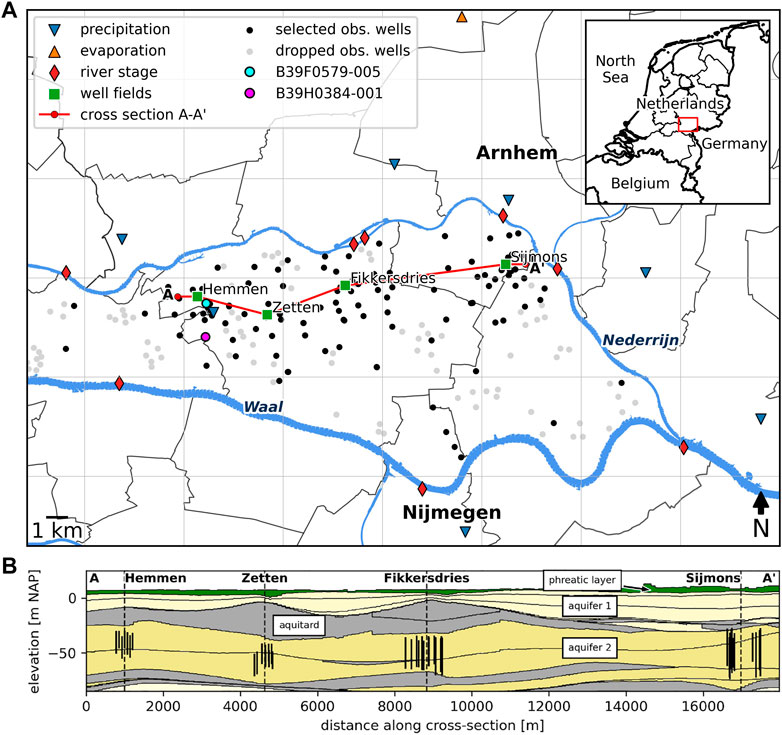
FIGURE 3. Overview of study area with locations of observation wells, and locations at which stresses are measured (A). Cross-section of the subsurface along well fields showing well screens, aquifers and aquitards (B).

The shallow subsurface is characterized by a low-permeable phreatic layer consisting mostly of clay and clayey sand, underlain by two aquifers, separated by an aquitard (see Figure 3). The aquitard consists of clay with a thickness varying from 0 to 15 m. The groundwater is relatively shallow with the depth to water table varying between 0.8 and 4.2 m.

Heads are actively monitored at 213 observation wells in the study area, some measuring heads in multiple filters at different depths, resulting in 395 head time series. Heads are measured with automatic pressure loggers, with daily, or shorter, measurement intervals for the period 2004–2020. Head measurements prior to 2004 are manual measurements, which are available at lower frequencies for some of the wells.

Daily precipitation data is available at seven measurement stations in the region (KNMI, 2022). Daily Makkink reference evaporation (de Bruin and Lablans, 1998) is available at two automatic weather stations. Mean yearly precipitation for 1990–2021 is 850 mm/year while mean yearly reference evaporation is 584 mm/year.

The river stage is measured at 10-min intervals at eight observation stations along both rivers (Figure 3) (Rijkswaterstaat, 2022). The time series are resampled to daily mean values. The maximum recorded daily mean river stage in the period 1990–2021 is 15.8 m, while the minimum recorded stage is 2.9 m.

Drinking water is extracted from the second aquifer at four well fields, at depths between −28 m and −74 m. From west to east, the well fields are Hemmen, Zetten, Fikkersdries, and Sijmons (see Figure 3). The date when pumping started, the average well screen depth, and mean pumping discharge are summarized in Table 1.

TABLE 1

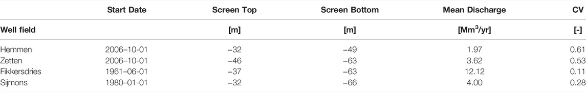
TABLE 1. Average pumping depth, pumping start date, mean discharge in the period 1990–2021, and the coefficient of variation (CV) for the four well fields. The coefficient of variation is calculated by dividing the standard deviation of the discharge by the mean discharge in the period 1990–2014.

3.1 Data Preparation

The calibration period was selected as 1990–2014 and the validation period as 2015–2021. All head data was pre-screened. Outliers were removed and head data was corrected for sudden unexpected jumps in the time series. Time series were discarded if they had fewer than 6 years with at least 180 measurements per year in the calibration period and/or fewer than one year of at least 180 measurements in the validation period. In addition, time series were discarded that visually showed a strong effect of the on- and off-switching of individual pumping wells in a well field. The resulting dataset consists of 250 head time series at 122 observation wells. Each head time series is assigned to one of the aquifers based on the observation depth.

The river stage is spatially interpolated at the point nearest to the observation well along the center line of the nearest river. Time series are calculated using a distance-weighted average between two observation stations. If the nearest point does not lie between two observation stations, the time series of the nearest observation station is used. The time series of the river stage is normalized by subtracting the mean.

The pumping data was resampled to obtain a time series of daily discharge for each well field. The available data was a mix of monthly (before 2007) and daily (after 2007) volumes. The time series prior to 2007 were converted to daily volumes by equally dividing the monthly volumes over each day in the month. The time series of daily pumping discharge for each well field are provided in the Supplementary Material (Supplementary Figure S1). The average location of all wells in a well field was used to measure the distance between a well field and an observation well (r in Eq. 6).

Heads are computed in the calibration period using daily data for all stresses. The noise model (Eq. 3) is rarely adequate for obtaining uncorrelated noise when using daily head observations, but works reasonably well for head data at 14-days intervals (e.g., Von Asmuth and Bierkens, 2005; Collenteur et al., 2021). The calibration data is obtained by taking a sample from each head time series on a 14-days interval within the calibration period.

4 Results

4.1 Example Results at One Observation Well

The results obtained for one observation well are discussed here in detail to illustrate the output of the time series model. Consider observation well B39F0579 (highlighted point in Figure 3), situated close to pumping station Hemmen (0.6 km) and at larger distances from stations Zetten (3.1 km) and Fikkersdries (7.1 km). Precipitation-excess, reference evaporation, river stage, and pumping rates from all three pumping wells are shown in Figure 4. Pumping at the well field in Fikkersdries started in the 1960s, before the start of the head observations. The pumping stations Hemmen and Zetten started operation in late 2006 with a relatively constant pumping rate until 2015, after which the pumping rate varied somewhat, with a significant increase in pumping in Hemmen in the last year of data. Observed heads in screen 5 of well B39F0579 (located in aquifer 2) are shown in the top graph of Figure 5. A clear decrease in head is visible from 2007 onwards, which coincides with the start of pumping. A further decline in heads is measured after 2015.

FIGURE 4

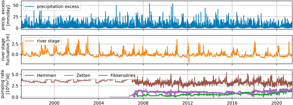
FIGURE 4. Stresses included in the time series model for observation well B39F0579 (Filter 5).

FIGURE 5

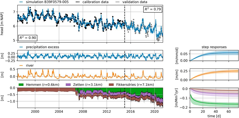
FIGURE 5. Contribution of the different stresses and the estimated step responses for the example model for observation well B39F0579 (Filter 5) in aquifer 2. The shaded areas around the step responses represent the 95% confidence intervals.

Time series models are developed with eight different model structures, as described in the previous section. Out of the 8 model structures, 6 model structures passed all four reliability checks. The selected best model structure includes precipitation-excess, the variation of the river stage, and three pumping wells. The results are shown in Figure 5. The simulated heads show a good fit with the data, as shown by a R² = 0.90 and R² = 0.79 in the calibration and the validation period respectively. During the validation period, the model overestimates the head in the summer months. These summers were particularly dry (e.g., Brakkee et al., 2022), and possibly stresses not included in the model (e.g., pumping for irrigation) could explain these deviations, but this has not been investigated here.

The contribution of each stress (precipitation excess, river stage, and pumping at the well fields) to the changes in head and their associated step response functions, as determined by the time series model, are shown in separate graphs in Figure 5. Up to 2006, the well field Fikkersdries caused a small drawdown that was stable over time. The drawdown caused by the other well fields started in late 2006 and stayed relatively constant until 2019, after which the drawdown increased as a result of increased pumping rates at Hemmen and to some extent Zetten. The total drawdown caused by all well fields exceeded 1 m after 2020, according to the model. The calibrated response functions (see plots on the right in Figure 5) are used to quantify the magnitude and timing of the drawdown caused by pumping from the three well fields.

4.2 Results for all Observation Wells

For each of the 250 head time series in the data set, 8 models with different structures were created and calibrated. The resulting 2000 time series models were evaluated and a best model structure was selected following the approach outlined in Figure 2. The total number of models that meet all four reliability criteria are presented in Table 2. 247 models for 129 unique head time series meet all four reliability criteria and are considered reliable. Some time series have multiple reliable models. For 121 (48%) time series no reliable model was present in the set of 8 model structures, and these time series are not considered further. Selection of the best model structure (according to the AIC) at each location, followed by a visual inspection, yields 126 (50%) reliable models that are used for further analysis. Out of these 126 models, 75 models include pumping at one or more well fields as a stress. Table 3 summarizes the model structures of the selected models, categorized per aquifer.

TABLE 2

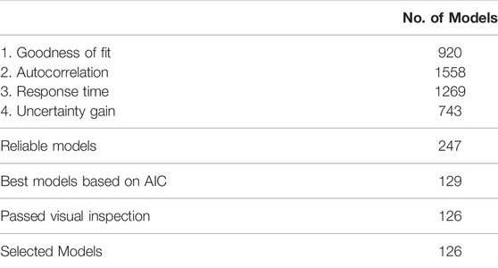
TABLE 2. Results for the reliability and selection criteria for all 2000 time series models for 250 locations.

TABLE 3

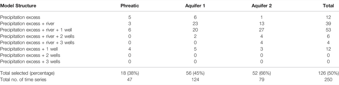
TABLE 3. Summary of model structures for selected time series models, counted per aquifer.

The steady-state drawdown caused by a well field is computed for all 75 observation wells where at least one well field has a significant effect on the head. The steady-state drawdown is computed using the average discharge of each well field for the period 2015–2021 and is plotted versus the distance between the observation well and the well field in Figure 6. The estimated steady-state drawdown in aquifer 2 shows a clear relationship with distance at well fields Hemmen, Zetten, and Sijmons. The estimated drawdown in aquifer 2 decreases with distance from those well fields (green symbols). There are insufficient models that meet all reliability criteria in aquifer 2 near well field Fikkersdries to discern any pattern.

FIGURE 6

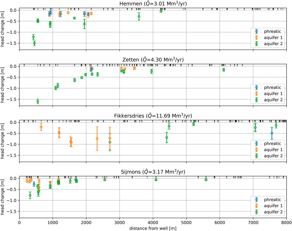
FIGURE 6. The estimated steady state head change versus the distance between the well field and the observation well using the average pumping rate $\left(\bar{Q}\right)$ between 2015 and 2020 for each well field. Uncertainty bars are 2 times the estimated standard deviation. The black ticks at the top of each graph indicate the distances at which an observation well is present but either none of the model structures was reliable or the well field was not included in the selected model structure.

In the phreatic layer and aquifer 1, no spatial pattern in drawdown is discernible. At Hemmen, the phreatic drawdown is in the same order of magnitude as the drawdown in aquifer 1. At Zetten, there are no models for observation well screens located in the top two layers within the first 2 km that passed all reliability criteria. At Sijmons, there are almost no models for phreatic observation wells and there is no discernible pattern in aquifer 1. The estimated steady state drawdown is much smaller in the top two layers, which are separated by an aquitard from the pumped aquifer. The vertical resistance of the aquitard is lowest around Hemmen and highest around Zetten (see Supplementary Figure S2 showing aquitard resistance in the Supplementary Material). This fits well with the results from time series analysis, where a significant effect of pumping was estimated in shallow observation wells near Hemmen, whereas this is not the case near Zetten.

The drawdown estimates near Fikkersdries show no consistent and plausible pattern. This may be explained through the historic development of pumping at this well field, which has been active since the early 1960s. In the period 2000–2021, the yearly pumping volumes have been relatively constant, varying between 10.5 and 13.6 Mm³/year. As such, the time series has a low coefficient of variation (CV, see Table 1) over the calibration period (CV = 0.11). In contrast, Hemmen (CV = 0.61) and Zetten (CV = 0.53) started pumping in 2006, and Sijmons (CV = 0.28) has seen a reduction in yearly pumping rate from around 5.5 Mm³/year to about 3 Mm³/year towards the end of the calibration period. The small variation in the pumping discharge at Fikkersdries makes it difficult to estimate the effect of pumping in observation wells.

5 Example Application: Timing and Magnitude of Drawdown at Hemmen

The time series analysis revealed a significant effect of pumping on the heads in 22 observation wells near the well field of Hemmen. Here, the effect of pumping on heads is compared per aquifer. Additionally, it is investigated whether low summer groundwater tables may be mitigated by reducing the pumping rate. Before implementing a potential mitigation measure, a decision-maker would need to determine the effectiveness of such a measure. Information on the magnitude and timing of the head response to reduced pumping is required for this purpose. This information is contained in the response functions associated with the pumping stresses.

The estimated step responses are plotted for all models that include pumping at Hemmen as a stress in Figure 7. The step responses are scaled with the gain for comparison purposes. The responses in aquifer 2 are the fastest because the well fields pump from the second aquifer. The responses in the phreatic observation wells are the slowest and show a 15–30-days lag after the start of pumping. Using these results, specifically the magnitude and the timing of the estimated head response to pumping, a decision-maker can determine the effectiveness of reduced pumping as a mitigation measure and what type of pumping strategy is potentially feasible.

FIGURE 7

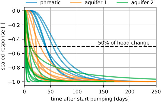
FIGURE 7. Scaled step responses for well field Hemmen, categorized per aquifer.

The response time, represented by the t₅₀, is plotted versus the distance from well field Hemmen in Figure 8 for each aquifer. The t₅₀ is a linear function of the distance from the well field (Eq. 8) for constant values of the fitting parameters a and b in the response function (Figure 1). The response times in the second aquifer are the shortest, ranging from about 1 to 11 days. The model at about 2000 m from Hemmen shows a larger uncertainty than other points, casting some doubt on the estimation of the response for this model. In the first aquifer the t₅₀ varies between 1 and 30 days. For the five observation wells in the phreatic layer, the t₅₀ is between 30 and 60 days. This means that 50% of the maximum reduction in drawdown as a result of a change in pumping rate takes 30–60 days to manifest itself in the phreatic layer. The estimated uncertainties are larger in more shallow aquifers. The general trend is that the independently estimated t₅₀ response times increase with the distance, as would be expected, though individual models do show significant variation.

FIGURE 8

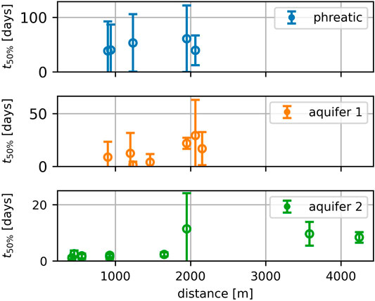
FIGURE 8. Estimated 50% response time for observations wells near well field Hemmen including estimated uncertainty (2σ).

The timing of the response of the phreatic layer to pumping at Hemmen means that reduction in pumping informed by weather forecasts (typically available for a 14-day period) to mitigate low groundwater tables in the summer would not be an effective mitigation measure at Hemmen. As an alternative, a systematic reduction in summer pumping is considered.

Two hypothetical pumping regimes are compared to investigate the effect of reduced pumping during the summer months on the heads. The first regime is a constant pumping rate of 6 Mm³/year. The second regime pumps 7 Mm³/year for 9 months per year and a reduced rate of 3 Mm³/year for three months. The total yearly production volume is equal in both scenarios, and equal to the current permit (6 Mm³/year). The pumping is reduced in the months May, June, and July such that the drawdown is minimized in June, July, and August, traditionally the driest months in the Netherlands. This variable pumping regime requires additional pumping at, e.g., well field Zetten to compensate for the reduction in drinking water production at Hemmen during the dry summer months. Whether this compensation can be realized in practice is outside the scope of this research.

Figure 9 shows the drawdown calculated with the response function for well field Hemmen for observation well B39H0384-001 (see highlighted point in Figure 3) for both pumping regimes, including a 95% confidence interval based on estimated parameter uncertainties. The drawdown at a constant pumping rate of 6 Mm³/year is 37 cm (with a relatively large 95% confidence interval of 8–45 cm). By reducing the pumping rate from May to July, the drawdown can be reduced in the summer. The maximum effect occurs in August, when the drawdown is reduced to 20 cm (with a 95% confidence interval of 5–27 cm), a reduction of 17 cm as compared to the constant pumping scenario. There is a 5 cm larger drawdown outside the summer months as a result of the increased pumping rate in those periods. The reduction in drawdown caused by the variable pumping regime for all five observation wells is shown in the bottom graph of Figure 9. The effect of the variable pumping regime is similar in all observation wells. The largest effect occurs in August and the maximum drawdown reduction varies between 10 and 17 cm.

FIGURE 9

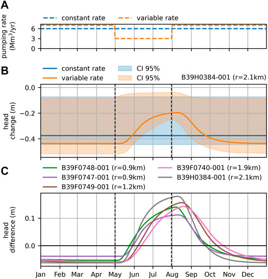
FIGURE 9. Comparison of the effect of two pumping regimes (A) on the calculated drawdowns for well B39H0384 (B) and the differences between calculated drawdowns corresponding to different pumping regimes for all 5 phreatic models (C). The drawdown is calculated using the derived response to pumping at well field Hemmen. The shaded areas represent the 95% confidence intervals.

6 Discussion

The objective of this paper is to develop and apply a data-driven, reproducible, and robust approach to estimate drawdowns as a result of pumping at multiple well fields. The proposed method is based on time series models that are derived exclusively from commonly observed data. The models can be constructed in a limited amount of time with low input data requirements. The described approach is implemented in Python scripts using the open-source software Pastas (Collenteur et al., 2019) to ensure full transparency and reproducibility.

The challenge of any modeling study is that a number of more-or-less subjective modeling decisions must be made. In the following, five major challenges are discussed:

1) Selection of the time periods used for model calibration and validation. A validation period is potentially valuable to test model performance, but the downside is that there is less data available for calibration. Shen et al. (2022) even propose skipping model validation entirely, based on a study of river discharge data in the United States. In the current study, the validation period (2015–2021) contains the driest years on record while at the same time the pumping stations of Hemmen and Zetten show a distinct increase in pumping rates (see Figure 4). This dry period may contain information of the head response that is not present in the calibration data. Exclusion of this period from the calibration period means the models might not be able to simulate these periods accurately. On the other hand, if models perform well despite this choice, this is a strong indication that the models are performing well for the right reasons. The mean R² for the selected models in the calibration period is 0.82 and 0.66 in the validation period. Good performance in the validation periods suggests the method and the models are robust. A robust method should yield the same model structure while a robust model should not produce significantly different estimates for the drawdown for an extension of the calibration period.

2) Time interval between head observations. A related challenge was the selection of the time interval between head observations used for model calibration. Higher frequency observations (i.e., daily) mean faster processes are captured by the data, potentially providing additional information to quantify the effects of the different stresses (Kavetski et al., 2011). However, the use of high frequency data increases the autocorrelation in the model residuals, troubling the estimation of parameter uncertainties. Reliable estimates of the parameter standard errors are important in this study, because they are used in the reliability criteria. Theoretically, autocorrelation can be reduced by improving the input data, improving the deterministic model, and/or improving the noise model. There is probably a point, however, where more head observations introduce more problems (e.g., autocorrelation) than they solve (e.g., better models). Different frequencies (daily, weekly, bi-weekly) of head observations were evaluated to calibrate the models (following Collenteur et al., 2021). A time interval of 14 days yielded good models while greatly reducing the number of models with significant autocorrelation in the noise. As a result, 1558 out of 2000 models (78%) passed the autocorrelation check, showcasing the effectiveness of the AR(1) noise model for data at a 14-days interval. The robustness of the method and the models to a different sample of head observations was tested by shifting the sample by 7 days and comparing the results visually. This led to somewhat different drawdown estimates for some models, but most models showed no significant changes in the estimated drawdowns. This analysis can be repeated 14 times to give additional insight into the robustness of the method to the selected sample of head observations (as was done by Collenteur et al., 2021).

3) Goodness-of-fit criterion. One of the four reliability criteria is the goodness-of-fit criterion that R² ≥ 0.7 (Figure 2). This is obviously a subjective criterion. It basically means that the model must fit the data reasonably well. It is unclear whether this requirement is really necessary. Other studies, for example Zaadnoordijk et al. (2019), opted for a much lower R² cutoffs of 0.1–0.3. When the R² criterion is dropped entirely, the number of observations wells where at least one model structure passes the three remaining reliability criteria, increases from 50 to 85%. The underlying question is whether the drawdown of the well fields can be estimated with sufficient accuracy even though the model fits the data poorly. Further research is needed to determine whether, and under what conditions, a goodness-of-fit criterion is needed to estimate the drawdown accurately.

4) Selection of the best model structure. The minimum AIC was used to select the best model structure from all reliable model structures for an observed head time series. In some cases, the differences in AIC values for different model structures were smaller than 2, meaning that multiple model structures are potentially supported by the data (Burnham et al., 2011). This introduces an uncertainty to the model selection step that was not taken into account in this study. Other methods of selecting the best model structure were considered, such as the model goodness-of-fit in the validation period, but occasional dubious observation data in the validation period, or minute differences in model performance, sometimes resulted in the selection of the model with the most parameters, while this did not seem to be warranted.

5) Visual inspection. Visual inspection of model performance in the validation period was deemed necessary as a last step in the selection process. A visual inspection remains valuable to identify models that show odd results, even though they pass all criteria, but a visual inspection is subjective as it is based on the expertise of the modeler. It is desirable to eliminate this subjective step, but this requires additional reliability criteria or fine-tuning of current criteria to local conditions. In each of the three cases where a model was rejected based on visual inspection, the t₉₅ of the response to river stage exceeded several years, but was not long enough to be rejected by the model reliability criteria. The model used the long response time to simulate a long-term trend in the data. For this specific study site, an additional reliability criterion can be added to limit the response time of changes in river stage, as such eliminating the necessity for visual inspection. This was not done, however, as such a criterion is applicable only for this local situation, while the four reliability criteria presented in Figure 2 are broadly applicable.

In groundwater hydrology, drawdowns of well fields are commonly estimated with physically-based groundwater models that are calibrated against head observations by adjusting the (spatial distribution) of the aquifer parameters. As a result, the estimated drawdowns make hydrological sense, as they are derived from basic principles such as continuity of flow and Darcy’s law. The approach presented in this paper is fully data-driven. The drawdown is estimated independently at each observation well using physically-based response functions. Each model had to pass four reliability checks and the uncertainty of the modeled drawdowns was estimated and plotted (e.g., Figure 6). The resulting spatial pattern of drawdowns makes hydrological sense, with drawdowns decreasing within a limited distance from a pumping station. Collenteur et al. (2019) applied a similar approach for single well fields and showed for an example application in the Netherlands that the drawdowns estimated with time series analysis compared well with the results of an analytic element model.

Application of time series analysis has been shown to be a viable method to estimate drawdowns, for example, through the use of synthetic data generated with a MODFLOW model (Shapoori et al., 2015). The same study also showed, however, that drawdown estimates can be biased if important processes (e.g., groundwater evaporation) are not taken into account in the model. In the current paper, eight different model structures were tested for each observation well. Different models to compute groundwater recharge (e.g., nonlinear approaches, Peterson and Western, 2014) were not considered, because a linear precipitation-excess model is commonly adequate to simulate head time series with 14-days time intervals in the Netherlands. A final uncertainty in the estimated drawdowns is the possible impact of unknown stresses. For example, pumping for irrigation probably occurs in the area during dry summers. Irrigation wells are largely unmetered, however, so that they can not be included in the model. This may affect the estimated drawdowns, but this is not any different from the application of a physically-based groundwater model.

A reproducible and transparent workflow was presented to develop reliable time series models. Application of this workflow at the study site resulted in reliable models for approximately 50% of the observed head time series. As mentioned above, the goodness-of-fit criterion was responsible for most of the rejections. It is the experience of the authors that a 50% success rate is pretty common in the modeling of transient flow. For example, Zaadnoordijk et al. (2019) obtained 47% decent or good time series models, according to their criteria. There are numerous reasons that can lead to a poor fit varying from data errors and missing stresses to inadequate model structures or local phenomena that affect the head variations. Additional research is needed to increase the percentage of successful models.

7 Conclusion

A reproducible, data-driven approach using open-source software is proposed to quantify the effects of different hydrological stresses on heads. A new method was developed to estimate the drawdown caused by pumping at multiple well fields. The data and the code for (re)producing the results presented in this study are available from a dedicated Zenodo repository (Brakenhoff et al., 2022). The method is able to derive reliable models for 50% (126) of the 250 considered head time series and quantify the effect of one or multiple well fields for 78 head time series.

The relative simplicity of the time series models allows the modeler to test multiple model structures (such as stresses and response functions) and model settings (such as the time interval between observations, and the calibration and validation periods) in a short amount of time. This quickly yields valuable insights into the driving hydrological processes affecting the head variations. The data-driven nature of the approach avoids the many approximations that have to be made when analyzing a similar problem using more traditional modeling techniques (e.g., numerical groundwater models). Each time series model is valid only at the specific location of the observation well where the heads are measured. Results at multiple observation wells show clear spatial patterns: drawdowns are larger in the pumped aquifers and decrease with distance from the well field while response times increase with distance from the well field, even though the data at each observation well is analyzed independent from the other observation wells.

The example application at well field Hemmen shows how time series models can be used to estimate the effects of the well field, both spatially and over time. Reduced pumping in May-July can reduce drawdown by about 10–20 cm in the summer months June-August. This is valuable information for decision-makers weighing potential strategies for mitigating low groundwater tables in dry periods.

Data Availability Statement

The datasets presented in this study can be found in an online repository. The name of the repository and accession number can be found at: https://zenodo.org/record/6372578#.YkLTyy8Rr0o.

Author Contributions

DB is the lead author, and performed the analysis presented in this paper together with MV. RC and MB contributed significantly with helpful advice throughout, and helped in writing the paper. MvB was involved in reviewing the application of simulating multiple wells with a single response function during the development stage.

Funding

The work from Raoul Collenteur was funded by the Austrian Science Fund (FWF) under Research Grant W1256 (Doctoral Program Climate Change: Uncertainties, Thresholds and Coping Strategies).

Conflict of Interest

DB, MV, and MvB were employed by the company Artesia B.V.

The remaining authors declare that the research was conducted in the absence of any commercial or financial relationships that could be construed as a potential conflict of interest.

Publisher’s Note

All claims expressed in this article are solely those of the authors and do not necessarily represent those of their affiliated organizations, or those of the publisher, the editors and the reviewers. Any product that may be evaluated in this article, or claim that may be made by its manufacturer, is not guaranteed or endorsed by the publisher.

Acknowledgments

The authors would like to acknowledge the drinking water supply company Vitens, who allowed us to publish this work using their data. Specifically we want to acknowledge Jelle van Sijl who initiated the project that eventually led to this paper, and was helpful throughout, by providing data, advice, and valuable insights into the complexities of drinking water production. The authors would also like to acknowledge Jeroen Castelijns from Brabant Water, for initiating the project in which the method for simulating multiple well fields with a single response function was developed.

Supplementary Material

The Supplementary Material for this article can be found online at: https://www.frontiersin.org/articles/10.3389/feart.2022.907609/full#supplementary-material

References

Akaike, H. (1974). A New Look at the Statistical Model Identification. IEEE Trans. Autom. Contr. 19, 716–723. doi:10.1109/TAC.1974.1100705

CrossRef Full Text | Google Scholar

Anderson, M. P., Woessner, W. W., and Hunt, R. J. (2015). Applied Groundwater Modeling: Simulation of Flow and Advective Transport. San Diego: Academic Press.

Google Scholar

Bakker, M., and Schaars, F. (2019). Solving Groundwater Flow Problems with Time Series Analysis: You May Not Even Need Another Model. Groundwater 57, 826–833. doi:10.1111/gwat.12927

PubMed Abstract | CrossRef Full Text | Google Scholar

Brakenhoff, D., Vonk, M., van Baar, M., Collenteur, R., and Bakker, M. (2022). Supplementary materials to ”Brakenhoff et al., Application of time series analysis to estimate drawdowns from multiple well fields. [Dataset]. doi:10.5281/zenodo.6372578

CrossRef Full Text | Google Scholar

Brakkee, E., van Huijgevoort, M. H. J., and Bartholomeus, R. P. (2022). Improved Understanding of Regional Groundwater Drought Development through Time Series Modelling: The 2018-2019 Drought in the Netherlands. Hydrol. Earth Syst. Sci. 26, 551–569. doi:10.5194/hess-26-551-2022

CrossRef Full Text | Google Scholar

Burnham, K. P., Anderson, D. R., and Huyvaert, K. P. (2011). AIC Model Selection and Multimodel Inference in Behavioral Ecology: Some Background, Observations, and Comparisons. Behav. Ecol. Sociobiol. 65, 23–35. doi:10.1007/s00265-010-1029-6

CrossRef Full Text | Google Scholar

Collenteur, R. A., Bakker, M., Caljé, R., Klop, S. A., and Schaars, F. (2019). Pastas: Open Source Software for the Analysis of Groundwater Time Series. Groundwater 57, 877–885. doi:10.1111/gwat.12925

PubMed Abstract | CrossRef Full Text | Google Scholar

Collenteur, R. A., Bakker, M., Klammler, G., and Birk, S. (2021). Estimation of Groundwater Recharge from Groundwater Levels Using Nonlinear Transfer Function Noise Models and Comparison to Lysimeter Data. Hydrol. Earth Syst. Sci. 25, 2931–2949. doi:10.5194/hess-25-2931-2021

CrossRef Full Text | Google Scholar

de Bruin, H. a. R., and Lablans, W. N. (1998). Reference Crop Evapotranspiration Determined with a Modified Makkink Equation. Hydrol. Process. 12, 1053–1062. doi:10.1002/(SICI)1099-1085(19980615)12:7<1053::AID-HYP639>3.0.CO;2-E

CrossRef Full Text | Google Scholar

Fienen, M. N., and Bakker, M. (2016). HESS Opinions: Repeatable Research: What Hydrologists Can Learn from the Duke Cancer Research Scandal. Hydrol. Earth Syst. Sci. 20, 3739–3743. doi:10.5194/hess-20-3739-2016

CrossRef Full Text | Google Scholar

Hantush, M. S., and Jacob, C. E. (1955). Non-steady Radial Flow in an Infinite Leaky Aquifer. Trans. AGU 36, 95–100. doi:10.1029/TR036i001p00095

CrossRef Full Text | Google Scholar

Hipel, K. W., and McLeod, A. I. (1994). “Chapter 7 Diagnostic Checking,” in Time Series Modelling of Water Resources and Environmental Systems (Amsterdam: Elsevier), 45, 235–253. Developments in Water Science. doi:10.1016/S0167-5648(08)70665-8

CrossRef Full Text | Google Scholar

Hugman, R., and Doherty, J. (2022). Complex or Simple-Does a Model Have to Be One or the Other? Front. Earth Sci. 10, 867379. doi:10.3389/feart.2022.867379

CrossRef Full Text | Google Scholar

Kavetski, D., Fenicia, F., and Clark, M. P. (2011). Impact of Temporal Data Resolution on Parameter Inference and Model Identification in Conceptual Hydrological Modeling: Insights from an Experimental Catchment. Water Resour. Res. 47, W05501. doi:10.1029/2010WR009525

CrossRef Full Text | Google Scholar

KNMI (2022). Dagwaarden Van Weerstations. [Dataset]. Available at: https://www.daggegevens.knmi.nl/klimatologie/daggegevens. (Febuary 22, 2022).

Google Scholar

Mackay, J. D., Jackson, C. R., and Wang, L. (2014). A Lumped Conceptual Model to Simulate Groundwater Level Time-Series. Environ. Model. Softw. 61, 229–245. doi:10.1016/j.envsoft.2014.06.003

CrossRef Full Text | Google Scholar

Obergfell, C., Bakker, M., Zaadnoordijk, W. J., and Maas, K. (2013). Deriving Hydrogeological Parameters through Time Series Analysis of Groundwater Head Fluctuations Around Well Fields. Hydrogeol. J. 21, 987–999. doi:10.1007/s10040-013-0973-4

CrossRef Full Text | Google Scholar

Patle, G. T., Singh, D. K., Sarangi, A., Rai, A., Khanna, M., and Sahoo, R. N. (2015). Time Series Analysis of Groundwater Levels and Projection of Future Trend. J. Geol. Soc. India 85, 232–242. doi:10.1007/s12594-015-0209-4

CrossRef Full Text | Google Scholar

Peterson, T. J., and Western, A. W. (2014). Nonlinear Time-Series Modeling of Unconfined Groundwater Head. Water Resour. Res. 50, 8330–8355. doi:10.1002/2013WR014800

CrossRef Full Text | Google Scholar

Rijkswaterstaat (2022). Waterhoogten (Expert). [Dataset]. Available at: https://waterinfo.rws.nl/#!/kaart/Waterhoogten/. (Febuary 22, 2022).

Google Scholar

Shapoori, V., Peterson, T. J., Western, A. W., and Costelloe, J. F. (2015). Decomposing Groundwater Head Variations into Meteorological and Pumping Components: A Synthetic Study. Hydrogeol. J. 23, 1431–1448. doi:10.1007/s10040-015-1269-7

CrossRef Full Text | Google Scholar

Shen, H., Tolson, B. A., and Mai, J. (2022). Time to Update the Split‐Sample Approach in Hydrological Model Calibration. Water Resour. Res. 58, e2021WR031523. doi:10.1029/2021WR031523

CrossRef Full Text | Google Scholar

Van Loon, A. F., Stahl, K., Di Baldassarre, G., Clark, J., Rangecroft, S., Wanders, N., et al. (2016). Drought in a Human-Modified World: Reframing Drought Definitions, Understanding, and Analysis Approaches. Hydrol. Earth Syst. Sci. 20, 3631–3650. doi:10.5194/hess-20-3631-2016

CrossRef Full Text | Google Scholar

Veling, E. J. M., and Maas, C. (2010). Hantush Well Function Revisited. J. Hydrol. 393, 381–388. doi:10.1016/j.jhydrol.2010.08.033

CrossRef Full Text | Google Scholar

Von Asmuth, J. R., and Bierkens, M. F. P. (2005). Modeling Irregularly Spaced Residual Series as a Continuous Stochastic Process. Water Resour. Res. 41, W12404. doi:10.1029/2004WR003726

CrossRef Full Text | Google Scholar

Von Asmuth, J. R., Bierkens, M. F. P., and Maas, K. (2002). Transfer Function-Noise Modeling in Continuous Time Using Predefined Impulse Response Functions. Water Resour. Res. 38, 23–31. doi:10.1029/2001WR001136

CrossRef Full Text | Google Scholar

Von Asmuth, J. R., Maas, K., Bakker, M., and Petersen, J. (2008). Modeling Time Series of Ground Water Head Fluctuations Subjected to Multiple Stresses. Groundwater 46, 30–40. doi:10.1111/j.1745-6584.2007.00382.x

CrossRef Full Text | Google Scholar

Von Asmuth, J. R., Maas, K., Knotters, M., Bierkens, M. F. P., Bakker, M., Olsthoorn, T. N., et al. (2012). Software for Hydrogeologic Time Series Analysis, Interfacing Data with Physical Insight. Environ. Model. Softw. 38, 178–190. doi:10.1016/j.envsoft.2012.06.003

CrossRef Full Text | Google Scholar

Wald, A., and Wolfowitz, J. (1940). On a Test whether Two Samples Are from the Same Population. Ann. Math. Stat. 11, 147–162. doi:10.1214/aoms/1177731909

CrossRef Full Text | Google Scholar

White, J. T., Foster, L. K., Fienen, M. N., Knowling, M. J., Hemmings, B., and Winterle, J. R. (2020). Toward Reproducible Environmental Modeling for Decision Support: A Worked Example. Front. Earth Sci. 8, 50. doi:10.3389/feart.2020.00050

CrossRef Full Text | Google Scholar

Wunsch, A., Liesch, T., and Broda, S. (2018). Forecasting Groundwater Levels Using Nonlinear Autoregressive Networks with Exogenous Input (NARX). J. Hydrol. 567, 743–758. doi:10.1016/j.jhydrol.2018.01.045

CrossRef Full Text | Google Scholar

Zaadnoordijk, W. J., Bus, S. A. R., Lourens, A., and Berendrecht, W. L. (2019). Automated Time Series Modeling for Piezometers in the National Database of the Netherlands. Groundwater 57, 834–843. doi:10.1111/gwat.12819

PubMed Abstract | CrossRef Full Text | Google Scholar