What Are the Principal Factors Affecting Ambient Ozone Concentrations in Czech Mountain Forests?

Introduction

Ground-level ozone (O₃), an important constituent of the atmosphere (Prinn, 2003; Singh and Fabian, 2003; Monks et al., 2015), belongs among the major factors exerting negative impacts on forests (Ferretti et al., 2015; EEA, 2016), and remains a challenging problem for current and future timber production and the conservation of natural plant communities, including species diversity (Krupa et al., 2001). A range of impacts due to elevated O₃ exposures have been reported by numerous authors, from changes in biochemical processes in living organisms to macroscopic injuries (e.g., Roschina and Roschina, 2003; Cape, 2008; Paoletti et al., 2010, etc.), although the field evidence for the impact of O₃ on forests remains less clear (Manning, 2005; De Vries et al., 2014; Cailleret et al., 2018).

The chemistry of O₃ is very complex (Finlayson-Pitts and Pitts, 1997; Seinfeldt and Pandis, 1998). Ozone is a product of the photochemical reactions of precursors, i.e., nitrogen oxides (NO_x), volatile organic compounds (VOC), methane (CH₄), and carbon monoxide (CO). Meteorology is strongly involved in O₃ formation, with atmospheric stability, high atmospheric pressure, high solar radiation, and air temperature as factors promoting O₃ buildup (Kovač-Andrič et al., 2009; Wang et al., 2017; Pyrgou et al., 2018). Many processes—physical, chemical, and biological—affect the formation, transportation, and destruction of O₃ and thus the final O₃ concentrations (Colbeck and Mackenzie, 1994; Seinfeldt and Pandis, 1998; Fowler et al., 2009). Ozone formation in the highly non-linear O₃-VOC-NO_x system is not yet fully understood (Sillman, 1999; Carillo-Torres et al., 2017).

Trends in O₃ are difficult to detect due to its large interannual variability (Jonson et al., 2006). The ambient O₃ in Europe has significantly decreased, though not as much as expected with respect to sharp reduction in precursor emissions since the 1990s (Sicard et al., 2013; Paoletti et al., 2014; Colette et al., 2017). It appears that the negative O₃ trend throughout Europe due to European emission controls has been counteracted by tendencies related to climate warming and the hemispheric transportation of pollutants from the source regions, such as Southeast Asia (Yan et al., 2018). Climate variability generally regulates the interannual variability in European O₃, whereas the changes in anthropogenic precursor emissions predominantly influence O₃ trends (Yan et al., 2018).

In order to better understand O₃ behavior, it is of major concern to identify the factors that account for most of the day-to-day variability in O₃ concentrations. Numerous studies have been published tackling this issue from various perspectives, using different approaches, examining diverse variables and their measures (e.g., Duenas et al., 2002; Tarasova and Karpetchko, 2003; Abdul-Wahab et al., 2005; Özbay et al., 2011). Regression-based approaches—with the most often used multiple linear regression analysis—are commonly used for modeling O₃ concentrations as a response variable, and with meteorological characteristics and different ambient air pollutants as explaining variables (e.g., Abdul-Wahab et al., 2005; Sousa et al., 2006; Pavón-Domínguez et al., 2014).

Ambient ozone levels in Czech Republic are high (Hůnová and Bäumelt, 2018). Exposures over Czech forests exhibit high year-to year variability (Hůnová et al., 2019), nevertheless they consistently exceed the critical level of 5 ppm h AOT40F (UN/ECE, 2004) since 1994, with peak values reaching 38–39 ppm h at some sites in different years. In some mountain forests, such as in the Jizerske hory Mts., the O₃ exposures are similar as in highly polluted sites in South Europe and higher altitudes (Hůnová et al., 2016). The critical level of 5 ppm h AOT40F is usually exceeded early in the growing season, generally in May (Hůnová and Schreiberová, 2012). The highest O₃ exposures, indicated by AOT40F, are permanently measured in south Czech Republic, the region much less affected by clouds, and thus receiving higher global radiation loads during growing seasons (Hůnová et al., 2019). Existing studies on O₃ biological effects on Czech forests are equivocal (Šrámek et al., 2007, 2012; Hůnová et al., 2010, 2011; Zapletal et al., 2012; Vlasáková-Matoušková and Hůnová, 2015), however, and despite the high O₃ levels recorded, no serious damage attributable to O₃ has been reported so far.

The aim of our study is to explore selected factors substantially affecting the day-to-day variability of O₃ concentrations in Czech mountain forests. In the effort to decrease O₃ levels, it is truly of the utmost importance to know how meteorology and emission precursors influence ozone in a quantitative way.

Methods

Sites and Period Under Review

We analyzed the observed data, recorded in regular long-term continuous monitoring at five mountain forest sites (Figure 1; Table 1) operated by the Czech Hydrometeorological Institute (CHMI). The sites under review are distributed unevenly across the territory of the Czech Republic (CR), and are situated in border mountains under different pollution loads: Krkonoše-Rýchory (KRK) and Souš (SOU) are situated in the northern CR; Rudolice v Horách (RUD) in the northwest CR, a region with cumulative major emission sources; Bílý Kříž (BKR) in the northeast CR in the highly polluted Silesia region; and Hojná Voda (HOJ) in the relatively unpolluted southern CR. All five measuring stations are situated in open areas. Nevertheless, in close vicinity of all these sites are extensive forested areas, covered predominantly by spruce forests (Picea abies). The KRK, BKR, and HOJ sites are roughly estimated to represent some tens to hundreds kilometers, whereas RUD and SOU sites represent somewhat less extensive regions, about several tens kilometers.

FIGURE 1

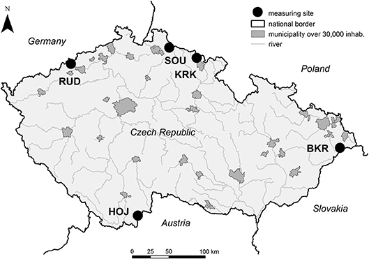
Figure 1. Measuring sites in map (the map was created in ArcGIS 10.3, based on ZABAGED layers, i.e., the geographic base data of the Czech Republic, belonging to information systems of the public service).

TABLE 1

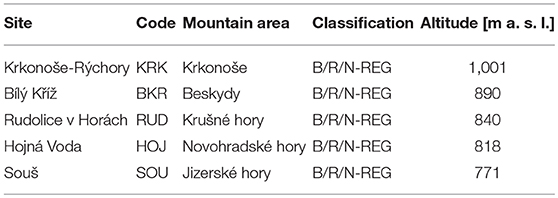
Table 1. Measuring sites - basic characteristics.

We examine the period of 1992–2018 (excluding days with missing ozone and/ or explanatory variables of our interest). This interval covers both the time with high emissions in the past (until 1998), and the “cleaner” period after profound socio-economic changes in Central Europe, including the CR, after the introduction of novel, more effective legislation for ambient air protection, and after the adoption of diverse countermeasures. From this 27-years record numerous data are missing, in different periods for individual sites. The NO_x ambient levels at four out of our five sites are available only until 2012. As a matter of fact, NO_x was monitored at Czech mountain sites only until 2012 (due to very low concentrations recorded in these areas previously), with the exception of BKR where NO_x monitoring continues. Table S1 presents an overview of the numbers of daily data at disposal for our analysis.

Input Data: Ambient Air Quality and Meteorology

The input data were retrieved from ISKO, the Czech nationwide ambient air quality database (CHMI, 2018b). All data we used were based on real-time, continuous measurements, from which 1 h averages were routinely calculated and stored—as the basic primary data—in ISKO database. With regard to quality of the dataset used: (1) the ambient O₃ and NO_x concentrations were checked thoroughly for gross errors by a database procedure based on mathematical and statistical methods (CHMI, 2018a), whereas (2) meteorology data, considered as support data, were checked only based on logic. The input data for all five sites run by the CHMI were measured by well-established, standardized methods as follows.

Ambient Ozone

We used the daily mean O₃ concentrations calculated from 1 h measurements, from the continuous, year-round, nationwide ambient air quality network. The measurement method was UV absorbance, the EC reference method (EC, 2008); the O₃ analyzers used were TEI-M49, manufactured by Thermo Environmental Instruments Inc., based in Franklin, Massachusetts, U.S. The sampling equipment was changed in 2015 to TAPI T-400, manufactured by Teledyne Advanced Pollution Instrumentation, Inc., based in San Diego, California, U.S. Standard QA/QC procedures in accordance with EU legislation (EC, 2008) were applied.

Nitrogen Oxides

We used the daily mean NO_x concentrations calculated from 1 h measurements, from the continuous, year-round, nationwide ambient air quality network. The measurement method was chemiluminescence, the EC reference method (EC, 2008); the NOx analyzers used were TEI–M42, manufactured by Thermo Environmental Instruments Inc., based in Franklin, Massachusetts, U.S. The sampling equipment was changed in 2015 to TAPI T-200, manufactured by Teledyne Advanced Pollution Instrumentation, Inc., based in San Diego, California, U.S. Standard QA/QC procedures in accordance with EU legislation (EC, 2008) were applied.

Meteorology

Meteorology monitored continuously with a 1 h time resolution was used. Namely, we used the daily mean air temperature, daily mean relative humidity, and daily global solar radiation (GLRD). The temperature in this paper is given in Kelvines [K]—this unit is used in our nation-wide database to avoid negative numbers, as negative numbers are exclusively assigned to error codes. Ambient air temperature in 2 m above ground and relative humidity were measured by Thies Clima HTT Compact, manufactured by Adolf Thies GmbH & Co., based in Gottingen, Germany. GLRD was measured by CMP sensors, manufactured by Kipp & Zonen B.V., based in Delft, The Netherlands. The meteorological variables were measured at the same sites and at the same hourly intervals as the air pollution variables.

Statistical Analysis

We have investigated the association between ambient O₃ concentrations on one hand, and precursor NO_x concentrations and meteorology on the other hand, using a generalized additive model, GAM (Wood, 2006). We accounted for NO_x as a proxy for ambient air pollution and a key player in O₃ chemistry. Unfortunately, VOCs as another key precursor group for O₃ formation could not be accounted for, as their concentrations are not recorded at the sites under review.

O₃ concentration was considered the dependent variable in the GAM model, whereas global solar radiation, air temperature, relative humidity, and NO_x concentrations were considered as explanatory variables. We worked with daily mean values calculated from primary 1 h values stored in a nationwide air-quality database. As the effects of some of these variables are known not to be linear, we used flexible GAM model formulation with semiparametric (penalized-spline-based) components to capture departures from linearity instead of forcing the relationship into the traditional but unrealistic linear (or log-linear) framework (Crawley, 2005). On the other hand, the GAM-retrieved relationships essentially reduce to linearity when the data do not support a non-linear relationship.

In order to maintain the comparability of results, the functional form of the GAM model is kept the same for all the sites we consider. Fitting was done separately for different sites (we stratified on site) so that we have site-specific parameters of the model with the same interpretation. For a given site, the GAM model is as follows:

$\begin{array}{l}{Y}_t={\beta }_0+s_T\left(Temperatur{e}_t\right)+s_G\left(GLR{D}_t\right)+s_H\left(Humidit{y}_t\right)\\ +s_{NOX}\left(NO{X}_t\right)+s_{TG}\left(Temperatur{e}_t,GLR{D}_t\right)+s_{TH}\\ \left(Temperatur{e}_t,Humidit{y}_t\right)+s_{GH}\left(GLR{D}_t,Humidit{y}_t\right)+{\epsilon }_t\end{array}$

where:

• Y_t is the daily mean ozone concentration for day t (time is indexed by the number of days since the first day of the data),

• β is an unknown constant (intercept) to be estimated from the data

• Temperature_t is the mean temperature for day t,

• GLRD_t is the mean GLRD for day t,

• Humidity_t is the mean relative humidity for day t,

• NOX_t is the mean NO_x concentration for day t,

• ε_t is the random error term. We adopt a working assumption of ε_t ~N (0,σ²)${\epsilon }_t~N(0,{\sigma }^2)$, which is a normal, zero mean, homoscedastic distribution of errors,

• S_T is an unknown univariate function (of temperature as an argument), of which the form is to be estimated from the data. We estimate it as a penalized spline (regularizing wiggliness via the penalization of the integral of the squared second derivative with respect to temperature). By that, we allow for potentially non-linear, smooth shapes of (marginal) dependence of O₃ on temperature,

• S_G is an unknown univariate function (of GLRD) to be estimated from the data as a penalized spline,

• S_H is an unknown univariate function (of Humidity) to be estimated from the data as a penalized spline,

• S_NOX is an unknown univariate function (of NO_x) to be estimated from the data as a penalized spline,

• S_TG is an unknown bivariate function (of Temperature and GLRD) to be estimated from the data as a tensor product penalized spline. This term allows us to investigate the possible interaction of Temperature and GLRD in influencing ozone concentration (i.e., departures from the simple additive effects of Temperature and GLRD). In other words, this effect enables us to investigate how the effect of Temperature is modified by GLRD (or, equivalently, how the effect of GLRD is modified by Temperature),

• S_TH is an unknown bivariate function (of Temperature and Humidity) to be estimated from the data as a tensor product penalized spline. This term corresponds to the Temperature^*Humidity (parsimoniously formu-lated) interaction,

• S_GH is an unknown bivariate function (of GLRD and Humidity) to be estimated from the data as a tensor product penalized spline. This term corresponds to the GLRD^*Humidity (parsimoniously formulated) interaction.

All unknown model components are estimated simultaneously (the model is identified) by optimizing the penalized likelihood. Unknown penalty coefficients are obtained via generalized cross-validation. All modeling computations were done in R core (2008). Results with p ≤ 0.05 are considered statistically significant. In graphs, the estimated spline functions are supplemented with 95% confidence intervals (constructed in pointwise fashion, so that they do not claim simultaneous coverage).

When estimating the model, we use all days with available data for a given station. From the model-fitting point of view, data are available when O₃ and all explanatory variables (temperature, GLRD, humidity, NO_x) are available. When at least one of these variables is missing, the day effectively appears as missing (i.e., it is not used in the fitting). Since different stations had missing days at different time-points, the model was estimated on a somehow different set of times, assuming that the ozone-to-explanatory-variables relationship is homogeneous in time.

Results

Table 2 presents an overview of descriptive statistics calculated from the mean daily values for all considered variables at all five measuring sites. Figures 2, 3 present the dynamics in the response variable (given as annual median values of respective variable), i.e., ambient O₃ concentrations, and explanatory variables: air temperature, GLRD, relative humidity, and ambient NO_x concentrations at all five sites under review. Though we used data over the 1992–2018 time period in our model, the dynamics in the variables (Figures 2, 3) are shown only for 1996–2016 due to the fact that at the beginning of measuring period, many data are missing, which would misrepresent the annual median in graphs. The GAM model, however, can cope with the missing data automatically (assuming homogeneity of the O₃ relationship to the explanatory variables in time and missing at random, or the MAR mechanism (Little and Rubin, 2002). The year-to-year variability in O₃ is high; the median concentrations at individual sites range between 28 and 45 ppb with clear peaks at some sites in 2003 and 2006. In spite of a clear decrease in NO_x concentrations, the ambient O₃ levels apparently do not decrease accordingly. Annual median temperatures ranged between 277.5 and 282 K, GLRD between 74 and 200 W m⁻², and relative humidity between 74 and 98%.

TABLE 2

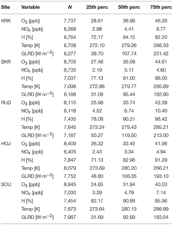
Table 2. Descriptive statistics for included variables at all five sites (calculated from daily data).

FIGURE 2

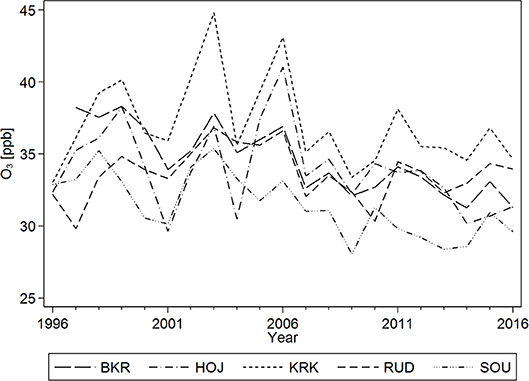
Figure 2. Trend in annual median ambient O₃ levels.

FIGURE 3

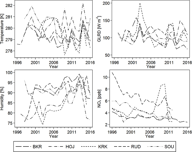
Figure 3. Trends in annual median air temperature, GLRD, relative humidity, and ambient NO_x concentrations.

The day-to-day variability in ambient O₃ concentrations is well described by a model including the additive effects of air temperature, GLRD, relative humidity, and ambient NO_x concentration, and the interactions of air temperature^*GLRD, air temperature^*relative humidity, and GLRD^*relative humidity (Figures 4–10). Though Figures 4–10 show the smooth terms with 95% confidence intervals from GAM model only for one site, namely BKR, the models for other four sites are looking quite similar. The relationship between O₃ expected value and temperature (Figure 4) shows higher O₃ values not only with higher temperatures, but, surprisingly, also with lower temperatures below 273.15 K (i.e., 0°C). Likely explanation for this finding rests in the fact that, mountain stations the data from which we analyze, are frequently above the inversion cloud layer in winter time, and receive high solar radiation capable of splitting the NO₂, a precursor molecule to O₃. Consequently, O₃ is recorded also in conditions of simultaneous low temperatures and high solar radiation, though O₃ levels are not that high as in summer when much higher temperatures promote O₃ formation reactions. The expected ozone value increases with increasing GLRD, though at some point the curve shows a plateau or even a slight decline (the decline is not significant, however, since it is outweighed by the increased variability) for higher GLRD values (Figure 5). Ozone concentration increases with decreasing relative humidity (Figure 6), right in line with physically-based intuition. The expected ozone value reaches its peak much more quickly than it decreases and shows a local maximum at about ambient NO_x concentration 3 ppb (Figure 7). Apart from the significant relationship between the response variable and individual explanatory variables, we also detected significant interactions between the three pairs of explanatory variables. Figure 8 shows the complex effect of interactions of air temperature^*GLRD upon the expected ambient O₃ concentration. Ozone evidently increases not only with increasing temperature and GLRD, which is a well-known fact, but also, surprisingly, with increasing GLRD at low temperatures. The dividing line is apparently around the ambient air temperature 280 K (i.e., 7°C). The ambient O₃ concentration generally increases with increasing temperature and decreasing humidity (Figure 9), whereas effect of interactions of relative humidity^*GLRD upon expected ambient O₃ concentration appears less straightforward (Figure 10). We can see a sharp increase of O₃ concentrations with decreasing relative air humidity at a GLRD around 250 W m⁻², whereas above that GLRD value, O₃ decreases.

FIGURE 4

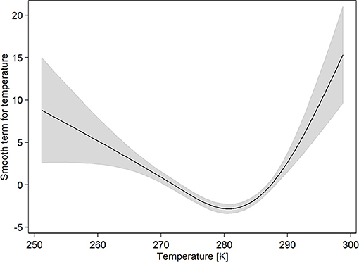
Figure 4. Effect of air temperature upon expected ambient O₃ concentration, BKR site.

FIGURE 5

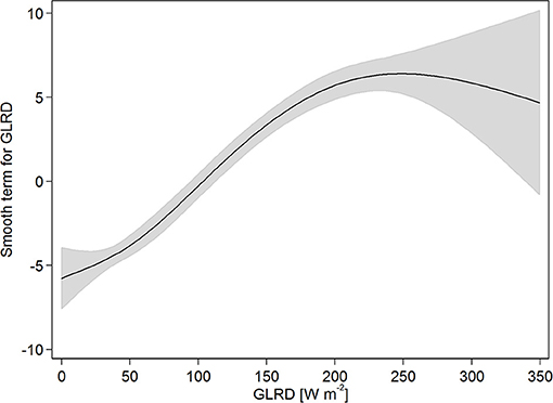
Figure 5. Effect of GLRD upon expected ambient O₃ concentration, BKR site.

FIGURE 6

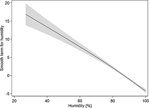
Figure 6. Effect of relative humidity upon expected ambient O₃ concentration, BKR site.

FIGURE 7

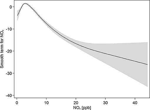
Figure 7. Effect of ambient NO_x concentrations upon expected ambient O₃ concentration, BKR site.

FIGURE 8

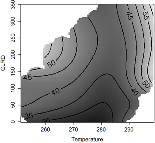
Figure 8. Effect of interactions of air temperature*GLRD upon expected ambient O₃ concentration, BKR site.

FIGURE 9

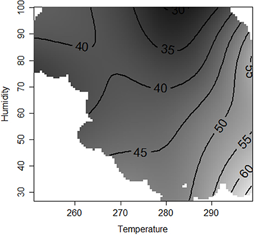
Figure 9. Effect of interactions of air temperature*relative humidity upon expected ambient O₃ concentration, BKR site.

FIGURE 10

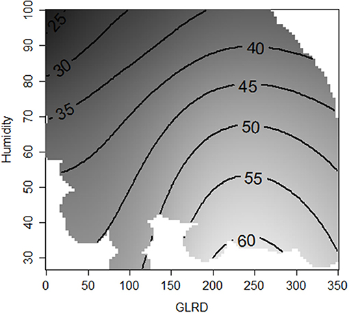
Figure 10. Effect of interactions of GLRD*relative humidity upon expected ambient O₃ concentration, BKR site.

The marginal effects of all selected explanatory variables are significant, but they differ in the strength of their effects upon ozone. All variables and their selected interactions are highly significant (p < 0.001) for all five sites, with a minor exception for the interaction of GLRD^*relative humidity for the KRK site, which is not significant, and for the BKR site with the p-value slightly less than the significance level of 0.05. The approximate significance of smooth terms is summarized in Table 3. At the KRK site, situated in the unpolluted top of the Krkonoše Mountains, influenced only by the long-range transport of air pollutants, all explanatory variables show similar strength, which also applies for interactions, which show a similar though lesser strength, as compared to the individual explanatory variables. A very similar pattern, though with a somewhat higher strength of relative humidity and lesser strength of air temperature, is obvious for the HOJ site, situated in the Novohradské hory Mountains, in the unpolluted (with regard to primary emissions and anthropogenic precursors of ambient ozone) south of the Czech Republic at the Austrian border. Ambient NO_x concentrations have a greater effect at sites representing more polluted regions. This holds true for the RUD site, situated at the Krusne hory mountain plateau and influenced by nearby large emission sources down in the valley (Bridges et al., 2002); for the SOU site, influenced by car exhaust from the nearby local road; and for the BKR site, influenced by emission sources in the polluted Silesian region (both on the Czech and the Polish sides of the border). The deviance explained for the individual sites is high, and ranges between 74.3% for the BKR and 63.4% for the SOU sites.

TABLE 3

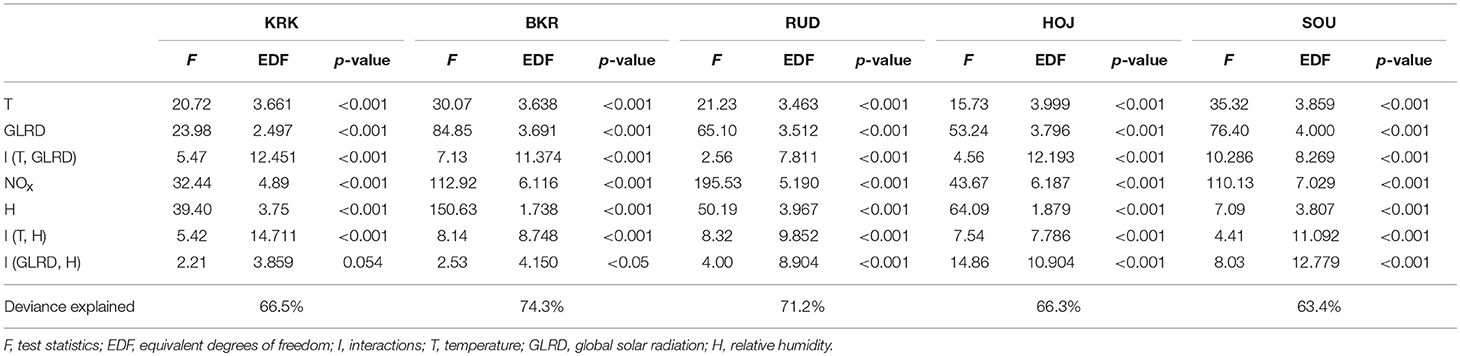
Table 3. Approximate significance of smooth terms.

Discussion

Complex Atmospheric Chemistry of O₃

Numerous studies examining O₃ chemistry, meteorology, and precursor emissions in Europe and North America, in different field research programs conducted under diverse geographical and climatic conditions, as well as studies of the combination of ground-based ozone data and meteorological observations, have resulted in enhancement of our knowledge of photochemical processes under various tropospheric conditions (Solomon et al., 2000; Monks et al., 2015). Nevertheless, it remains a challenge to interpret ambient O₃ behavior, levels, and trends. Atmospheric chemistry resulting in O₃ formation and destruction is, as a matter of fact, extremely complex due to numerous factors influencing these processes, and hence, O₃ concentrations (Cape, 2008).

Meteorology is extremely important for O₃ formation. It affects O₃ concentrations not only directly (via horizontal advection, vertical diffusion, and photolysis rates), but also indirectly, by influencing the concentrations of its precursors and chemistry of its formation and destruction (Oikonomakis et al., 2018). O₃ has a temperature-dependent chemistry (Pusede et al., 2015), and temperature was used in some studies as a surrogate to indicate O₃ formation via the O₃-temperature association, both at individual measuring sites and on a greater regional scale (Oikonomakis et al., 2018). The O₃-temperature relationship originates in: (1) temperature-dependent biogenic VOC emissions, (2) thermal decomposition of PAN to HO_x and NO_x, (3) increased likelihood of favorable meteorological conditions for ozone formation (Abeleira and Farmer, 2017). However, there are major uncertainties in the mechanisms underlying the temperature-dependent changes in O₃ concentrations, their interactions, and relative contributions in rural and remote regions (Romer et al., 2018). Ozone chemistry regimes are shifting as precursor emissions are changing (Abeleira and Farmer, 2017). Moreover, meteorology-dependent O₃ chemistry implicates the impact of ongoing climate change on O₃. Increasing temperature is expected to increase O₃ concentrations (Abeleira and Farmer, 2017). Additionally, the projected rise in global precursor emissions over the twenty-first century is also assumed to have a strong effect on O₃ throughout the world (Vingarzan, 2004). In contrast to temperature, field studies on GLRD influence on ground-level O₃ concentrations are scarce (Duenas et al., 2002). Though it is a well-known fact, that ambient O₃ is strongly dependent on GLRD (Finlayson-Pitts and Pitts, 1997; Seinfeldt and Pandis, 1998), some authors showed that solar radiation had a lower effect than expected upon O₃ concentrations as compared to more important effect of temperature (Abdul-Wahab and Al-Alawi, 2002).

The association between meteorological factors, precursor emissions, and O₃ daily variability might differ in urban and rural areas. Whereas the precursor emissions used to be much higher in urban areas, in rural regions the precursors are lower, in particular with respect to NO_x (Romer et al., 2018). Most papers on this issue examine the O₃ regime in urban areas (e.g., Duenas et al., 2002; Tan et al., 2018), whereas the papers on rural regions are less frequent (e.g., Pudasainee et al., 2006).

Strengths and Weaknesses of the GAM Model Used

Various statistical approaches to model O₃ dependence on meteorology and ambient air pollutants have been employed recently and have been reviewed by Thompson et al. (2001) and Schlink et al. (2003). The main objectives are O₃ forecasting, estimating O₃ time trends, and investigating the underlying processes based on observation data. The input data may vary widely both in terms of the variables considered, and in terms of observation scales in space and time (Thompson et al., 2001). The multiple linear regression method is frequently used (e.g., Abdul-Wahab et al., 2005; Sousa et al., 2006; Pavón-Domínguez et al., 2014), though it encounters serious difficulties when the independent variables are correlated with each other, i.e., when they exhibit multicollinearity (Al-Alawi et al., 2008). This is exactly the case of O₃, when e.g., the explanatory variables of temperature and GLRD are correlated. One method used to remove this multicollinearity is principal component analysis (PCA), selecting variables with high loadings to be used as predictors in a regression equation (e.g., Rajab et al., 2013). In our data (and moderate number of explanatory variables), collinearity is not a problem. The variance inflation factor, VIF (Rawlings et al., 1998), is smaller than 2.5 at all five sites. Even more importantly, O₃ formation and destruction are complex non-linear processes, and principal component regression cannot adequately model the non-linear relationship (Al-Alawi et al., 2008), and hence it cannot be used to retrieve true functional relationships, only linear (often hard-to-interpret) approximation. Neural networks and generalized additive models are recommended to address this issue, as they can handle non-linear associations and can be adapted easily to site-specific conditions (Schlink et al., 2003), but since they are used in a black-box style, they are much more useful for prediction than for analysis purposes.

Since we used a rather flexible class of statistical models (Generalized Additive Model with penalized spline components), we allow for a smooth relationship between O₃ and explanatory variables (temperature, GLRD, humidity, and NO_X). This class would not be ideal for relationships showing very sharp bends, sudden jumps at particular values of covariates, etc. From the physical and chemical backgrounds of O₃ behavior, however, we do not expect this sort of behavior and take GAM as a tool allowing for non-linearity in explanatory variables (unlike standard multiple regression, which insists on linearity, i.e., on the gradient with respect to a given explanatory variable being constant throughout its range). Since we use tensor product splines, we can also assess possible interactions in influences of certain pairs of explanatory variables (i.e., to assess whether their influence is simply additive or more complicated). Since we concentrate only on two-variable interactions, we can assess not only their overall significance (via the p-values of formalized hypothesis tests), but also display the interactions in graphical form (as contour plots showing how the mean ozone concentration depends on a pair of explanatory variables).

Volatile Organic Compounds Are Lacking in Our Model

The weak point of our model is the fact that the VOCs, an important O₃ precursor group, are not included in our model. This is due simply to the fact that the measured data are not available. There are no significant anthropogenic sources of VOCs near the five mountain sites under review; nevertheless, the surrounding forests are undoubtedly a major source of natural biogenic VOCs (further, BVOCs). BVOCs are a large group of organic chemicals including isoprene, terpenes, fatty acid derivates, benzenoids, phenylpropanoids, and amino acid derived metabolites (Esposito et al., 2016). They are emitted into the atmosphere by plants, and significantly affect its chemical composition and physical properties (Laothawornkitkul et al., 2009; Pinto et al., 2010), contributing substantially, among other effects, to the oxidizing capacity of the atmosphere through the recycling of hydroxyl radicals, OH (Lelieveld et al., 2008). Interestingly, on a global scale, BVOC emissions exceed by far those emitted due to anthropogenic activities (Seinfeldt and Pandis, 1998), and are more reactive (Holzinger et al., 2005). BVOCs belong among the key players in ambient O₃ chemistry in rural areas (Atkinson and Arey, 2003; Di Carlo et al., 2004).

We assume that natural BVOCs at the investigated sites are very important, as all five sites under review are situated in the close vicinity of vast forested areas, with a clear predominance of Norway spruce (Picea abies). It has been widely accepted that the vegetative emissions display large inter-species and inter-individual variability (Aydin et al., 2014). As compared to some other woody species, such as poplar or beech, spruce is a lower BVOC emitter (Bortsoukidis et al., 2014); however, it is still known to emit considerable amounts of reactive trace gases, and is considered particularly as an emitter of monoterpenes, such as α-pinene, β-pinene, limonene, and myrcene, whereas it is only a low isoprene emitter (Esposito et al., 2016; Jurán et al., 2017). Though some indicative information exists on BVOC emission for the CR (Zemankova and Brechler, 2010; Jurán et al., 2017), observation-based data in high time-resolution suitable for use in our model are lacking at present. Nevertheless, it would be very interesting in the future to include the data on BVOC concentration to observe how they influence our model.

Relevance of Our Results to Forests

On a long-term basis, ambient O₃ has been considered as a stress factor contributing to impairment of forest health status and its influence has been studied from different aspects. In spite of clear evidence of O₃ harmful effects observed in laboratory experiments, fumigation chambers, or FO₃X (Free air O₃ eXposure) experiments (Sandermann et al., 1997; Paoletti et al., 2017; Franz et al., 2018; Hoshika et al., 2018), the field evidence for impacts of O₃ exposure on tree growth is not that clear (De Vries et al., 2014; Cailleret et al., 2018). Moreover, observations in real stand conditions from numerous regions show that measured high O₃ exposures or modeled high O₃ stomatal flux do not correspond with unclear impacts on forest ecosystems (e.g., Ferretti et al., 2007; Matyssek et al., 2007; Waldner et al., 2007; Baumgarten et al., 2009).

European-wide assessment shows that, ambient O₃ exposures recorded at Czech background rural sites are medium in European context, being lower than in Southern Europe including Mediterranean, but higher than in Scandinavia, similar as in Germany and Switzerland (e.g., Waldner et al., 2007; Baumgarten et al., 2009; EEA, 2016). In our earlier work we assessed long-term time trends and spatial variability in ambient O₃ concentrations throughout the Czech Republic (Hůnová and Bäumelt, 2018), O₃ exposure over Czech forested areas (Hůnová and Schreiberová, 2012), compared different GIS methods to create a reliable O₃ and AOT40F map based on observed data (Hůnová et al., 2012), studied O₃ exposure, stomatal flux, and ozone injury on native vegetation in mountain forests (Hůnová et al., 2011; Vlasáková-Matoušková and Hůnová, 2015; Hůnová, 2017), and indicated the Czech forest regions which are stressed by permanent high O₃ exposures (Hůnová et al., 2019).

In present study we have investigated exclusively the O₃ behavior with respect to its day-to-day response to selected meteorology characteristics and NO_x precursors. Our results confirmed non-linear behavior of ambient O₃ not only to NO_x precursors, which is a well-known fact (Finlayson-Pitts and Pitts, 1997; Seinfeldt and Pandis, 1998), but also to meteorology, including all variables considered. Our results thus point out to certain deficiency of models investigating the underlying processes of O₃ formation based on measured data not considering this non-linear behavior toward ambient air temperature, GLRD, and relative humidity. This might be beneficial, for example, in modeling future scenarios for forested regions, accounting for changes in ambient O₃ toward local ambient air temperature, GLRD and relative humidity. Furthermore, our results indicated the necessity of considering not only individual explaining variables but also their interactions, such as the interactions of air temperature^*GLRD, air temperature^*relative humidity, and GLRD^*relative humidity. This might be of high relevance in particular in context of global climate change (Bytnerowicz et al., 2007; Sicard et al., 2017). In this respect Czech Republic heads toward hotter and drier conditions (Hlásny et al., 2011; Trnka et al., 2015; Štěpánek et al., 2016), which is likely to affect future ambient O₃ concentrations. The associations indicated by our study might enhance the models estimating potential future impacts of environmental/ climate changes on forests.

Ambient O₃ is, alongside with nitrogen deposition, considered on a long-term basis as an important factor affecting negatively European forests (EEA, 2016). Nevertheless, in recent years, this factor has been in Central Europe and elsewhere overshadowed by two other major threats for forests, namely unprecedented drought and unprecedented bark beetle outbreaks (Allen et al., 2010). Forests with compromised ecological stability, such as traditional forest monocultures in particular, are especially prone to large scale damage (Hlásny and Turčáni, 2013). This holds for most of the Czech forests, which can be classified as managed low-diversity ecosystems (Vacek et al., 2013), with decreased stand stability in respect to damages caused by natural abiotic agents (wind, snow, glaze, drought), biotic factors (insects including bark-beetle, pathogens), and also by anthropogenic effects, such as ambient air pollution. This adverse development is manifested by recent unprecedented salvage felling in Czech forests (Pajtík et al., 2018; Zahradník and Zahradníková, 2019). That present Czech forest decline is a result of a complex interplay of multiple factors was stressed by several recent observation-based studies (Kolár et al., 2015; Cienciala et al., 2016; Altman et al., 2017).

Czech forests in history were substantially changing in terms of area, species representation, and tree age. Presently, out of 26,664 km² of forested area representing some 34% of the Czech territory, Norway spruce (Picea abies), traditionally an important timber tree, is still a dominant species covering ca. 51% of the total forested area, following pine trees (Pinus spp.) cover 17%, beech (Fagus sylvatica) 8%, and oak (Quercus spp.) 7% (Ministry of Agriculture, 2015). Spruce is a somewhat ambiguous species with respect to O₃ sensitivity—it is assumed not to be especially sensitive in relation to visible injury but regarded as O₃-sensitive in relation to growth responses (UN/ECE, 2004). Nevertheless, we have to keep on mind that ambient air pollution is a factor affecting forests. We have already witnessed earlier that, predisposition of Norway spruce by air pollution (namely by high ambient SO₂ concentrations in the 1970s and 1980s) to stress from climatic events, such as drought and temperature changes, resulted in forest decline in Czech Republic (Vacek et al., 2015).

Conclusions

The generalized additive model confirmed that selected explanatory variables, i.e., air temperature, GLRD, relative humidity, and NO_x, significantly affect daily O₃ concentrations in Czech forests. Apparently, both meteorology and air pollution are highly influential on day-to-day O₃ concentrations, and this finding is consistent for all five rural sites representing middle-elevated forested mountain areas in Central Europe. We believe it would be of the utmost importance to include BVOCs in our analysis. Nevertheless, at present this is impossible, as the relevant data for BVOCs for these sites do not exist. Additionally, in contrast to a standard approach based on multiple linear regression used for similar studies, we were able to access non-linear relationships of various covariates to ozone, and also to characterize the interactions of the three pairs of explanatory variables, namely temperature^*GLRD, temperature^*relative humidity, and GLRD^*relative humidity. We extracted functional relationship of various explanatory variables, demonstrating deficiencies of standardly used linear approximations. Local extrema visible in some of the bivariate relationships (O₃ to temperature or to NO_x) can, in addition to saturation (upper asymptote) visible in the relationship of O₃ to GLRD, easily distort quantification of covariate effects, e.g., to forests injury and/ or to smear out various climatic scenario comparisons based on standard linear approach. Non-linear relationships (qualitatively clear from the O₃ atmospheric chemistry) should be taken seriously also in real, observed data analysis. GAM methodology offers a powerful tool for this.

Author Contributions

IH coordinated the study. IH, MB, and MM contributed to the conception and design of the study. MM organized the database and prepared the final version of Figures 2–10. MB performed the statistical analysis. IH wrote the first draft of the manuscript. All authors contributed to manuscript revision, read, and approved the submitted version.

Funding

This work was partially supported by the long-term strategic development financing of the Institute of Computer Science (Czech Republic RVO 67985807).

Conflict of Interest Statement

The authors declare that the research was conducted in the absence of any commercial or financial relationships that could be construed as a potential conflict of interest.

Acknowledgments

We thank Erin Naillon for proofreading our manuscript and Jana Schovánková from the CHMI for preparing the Figure 1. We also appreciate the comments and suggestions of three reviewers, which enhanced our manuscript substantially.

Supplementary Material

The Supplementary Material for this article can be found online at: https://www.frontiersin.org/articles/10.3389/ffgc.2019.00031/full#supplementary-material

References

Abdul-Wahab, S. A., and Al-Alawi, S. M. (2002). Assessment and prediction of tropospheric ozone concentration levels using artificial neural networks. Environ. Model. Softw. 17, 219–228. doi: 10.1016/S1364-8152(01)00077-9

CrossRef Full Text | Google Scholar

Abdul-Wahab, S. A., Bakheit, C. S., and Al-Alawi, S. M. (2005). Principal component and multiple regression analysis in modelling of ground-level ozone and factors affecting its concentrations. Environ. Model. Softw. 20, 1263–1271. doi: 10.1016/j.envsoft.2004.09.001

CrossRef Full Text | Google Scholar

Abeleira, A. J., and Farmer, D. K. (2017). Summer ozone in the northern Front Range metropolitan area: weekend-weekday effects, temperature dependences, and the impact of drought. Atmos.Chem. Phys. 17, 6517–6529. doi: 10.5194/acp-17-6517-2017

CrossRef Full Text | Google Scholar

Al-Alawi, S. M., Abdul-Wahab, S. A., and Bakheit, C. B. (2008). Combining principal component regression and artificial neural networks for more accurate predictions of ground-level ozone. Environ. Model. Softw. 23, 396–403. doi: 10.1016/j.envsoft.2006.08.007

CrossRef Full Text | Google Scholar

Allen, C. D., Macalady, A. K., Chenchouni, H., Bachelet, D., McDowell, N., Vennetier, M., et al. (2010). A global overview of drought and heat-induced tree mortality reveals emerging climate change risks for forests. For. Ecol. Manage. 259, 660–684. doi: 10.1016/j.foreco.2009.09.001

CrossRef Full Text | Google Scholar

Altman, J., Fibich, P., Santruckova, H., Dolezal, J., Stepanek, P., Hunova, I., et al. (2017). Environmental factors exert strong control over the climate-growth relationships of Picea abies in Central Europe. Sci. Total Environ. 609, 506–516. doi: 10.1016/j.scitotenv.2017.07.134

PubMed Abstract | CrossRef Full Text | Google Scholar

Atkinson, R., and Arey, J. (2003). Gas-phase tropospheric chemistry of biogenic volatile organic compounds: a review. Atmos. Environ. 37 (Suppl. 2), S1972–S219. doi: 10.1016/S1352-2310(03)00391-1

CrossRef Full Text | Google Scholar

Aydin, Y. M., Yaman, B., Koca, H., Dasdemir, O., Kara, M., Altiok, H., et al. (2014). Biogenic volatile organic compound (VOC) emissions from forested areas in Turkey: determination of specific emission rates for thirty-one tree species. Sci. Total Environ. 490, 239–253. doi: 10.1016/j.scitotenv.2014.04.132

CrossRef Full Text | Google Scholar

Baumgarten, M., Huber, C., Buker, P., Emberson, L., Dietrich, H.-P., et al. (2009). Are Bavarian forests (southern Germany) at risk from ground-level ozone? Assessment using exposure and flux based ozone indices. Environ. Pollut. 157, 2091–2107. doi: 10.1016/j.envpol.2009.02.012

CrossRef Full Text | Google Scholar

Bortsoukidis, E., Williams, J., Kesselmeier, J., Jacobi, S., and Bonn, B. (2014). From emissions to ambient mixing ratios: online seasonal field measurements of volatile organic compounds over a Norway spruce-dominated forest in central Germany. Atmos.Chem. Phys. 14, 6495–6510. doi: 10.5194/acp-14-6495-2014

CrossRef Full Text | Google Scholar

Bridges, K. S., Jickells, T. D., Davies, T. D., Zeman, Z., and Hůnová, I. (2002). Aerosol, precipitation and cloud water chemistry observations on the Czech Krusne hory plateau adjacent to a heavily industrialised valley. Atmos. Environ. 36, 353–360. doi: 10.1016/S1352-2310(01)00388-0

CrossRef Full Text | Google Scholar

Bytnerowicz, A., Omasa, K., and Paoletti, E. (2007). Integrated effects of air pollution and climate change on forests: a northern hemisphere perspective. Environ. Pollut. 147, 438–445. doi: 10.1016/j.envpol.2006.08.028

PubMed Abstract | CrossRef Full Text | Google Scholar

Cailleret, M., Ferretti, M., Gessler, A., Rigling, A., and Schaub, M. (2018). Ozone effects on European forest growth – towards an integrative approach. J. Ecol. 106, 1377–1389. doi: 10.1111/1365-2745.12941

CrossRef Full Text | Google Scholar

Cape, J. N. (2008). Surface ozone concentrations and ecosystem health: past trends and a guide to future projections. Sci. Total Environ. 400, 257–269. doi: 10.1016/j.scitotenv.2008.06.025

PubMed Abstract | CrossRef Full Text | Google Scholar

Carillo-Torres, E. R., Hernández- Paniagua, I. Y., and Mendoza, A. (2017). Use of combined observational- and model- derived photochemical indicators to assess the O₃-NO_x-VOC system sensitivity in urban areas. Atmosphere 8:22. doi: 10.3390/atmos8020022

CrossRef Full Text | Google Scholar

CHMI (Czech Hydrometeorological Institute) (2018a). Tabular Survey 2017. Prague: Czech Hydrometeorological Institute. Czech /English version. Avaliable online at: http://portal.chmi.cz/files/portal/docs/uoco/isko/tab_roc/2017_enh/index_GB.html

CHMI (Czech Hydrometeorological Institute) (2018b). Air Pollution in the Czech Republic in 2017. Prague: Czech Hydrometeorological Institute. Czech /English version. Avaliable online at: http://portal.chmi.cz/files/portal/docs/uoco/isko/grafroc/17groc/gr17cz/Obsah_CZ.html

Cienciala, E., Russ, R., Šantručková, H, Altman, J., Kopáček, J., Hůnová, I., et al. (2016). Discerning environmental factors affecting current tree growth in Central Europe. Sci. Total Environ. 573, 541–554. doi: 10.1016/j.scitotenv.2016.08.115

PubMed Abstract | CrossRef Full Text | Google Scholar

Colbeck, I., and Mackenzie, A. R. (1994). Air Pollution by Photochemical Oxidants. Amsterdam: Elsevier.

Google Scholar

Colette, A., Andersson, C., Manders, A., Mar, K., Mircea, M., Pay, M-T., et al. (2017). EURODELTA-Trends, a multi-model experiment of air quality hindcast in Europe over 1990−2010. Geoscient. Model Dev. 10, 3255–3276. doi: 10.5194/gmd-10-3255-2017

CrossRef Full Text | Google Scholar

Crawley, M. J. (2005). Statistics: An Introduction Using R. London: John Wiley & Sons, Ltd.

Google Scholar

De Vries, W., Dobbertin, M. H., Solberg, S., Van Dobben, H. F., and Schaub, M. (2014). Impacts of acid deposition, ozone exposure and weather conditions on forest ecosystems in Europe: an overview. Plant Soil 380, 1–45. doi: 10.1007/s11104-014-2056-2

CrossRef Full Text | Google Scholar

Di Carlo, P., Brune, W. H., Martinez, M., Harder, H., Lesher, R., Ren, X., et al. (2004). Missing OH reactivity in a forest: evidence for unknown reactive biogenic VOCs. Science 304, 722–725. doi: 10.1126/science.1094392

PubMed Abstract | CrossRef Full Text | Google Scholar

Duenas, C., Fernández, M. C., Canete, S., Caarretero, J., and Liger, E. (2002). Assessment of ozone variations and meteorological effects in an urban area in the Mediterranean cost. Sci. Total Environ. 299, 97–113. doi: 10.1016/S0048-9697(02)00251-6

CrossRef Full Text | Google Scholar

EC (2008). Directive 2008/50/EC of the European Parliament and of the Council of 21 May 2008 on Ambient Air Quality and Cleaner Air for Europe. OJEC L 152.

Google Scholar

EEA (2016). Air Quality in Europe – 2016 Report. Luxembourg: European Environment Agency.

Google Scholar

Esposito, R., Lusini, I., Večerová, K., Holišová, P, Pallozzi, E., Guidolotti, G., et al. (2016). Shoot-level terpenoids emission in Norway spruce (Picea abies) under natural field and manipulated laboratory conditions. Plant Physiol. Biochem. 108, 530–538. doi: 10.1016/j.plaphy.2016.08.019

PubMed Abstract | CrossRef Full Text | Google Scholar

Ferretti, M., Fagnano, M., Amoriello, T., Badiani, M., Ballarin-Denti, A., Buffoni, A., et al. (2007). Measuring, modelling and testing ozone exposure, flux and effects on vegetation in southern European conditions – What does not work? A review from Italy. Environ. Pollut. 146, 648–658. doi: 10.1016/j.envpol.2006.05.012

CrossRef Full Text | Google Scholar

Ferretti, M., Sanders, T., Michel, A., Calatayud, V., Cools, N., Gottardini, E., et al. (2015). The Impact of Nitrogen Deposition and Ozone on the Sustainability of European Forests. ICP Forests 2014 Executive Report, e-ISSN. 2198–6541.

Google Scholar

Finlayson-Pitts, B. J., and Pitts, J. N Jr. (1997). Tropospheric air pollution: ozone, airborne toxics, polycyclic aromatic hydrocarbons, and particles. Science 276, 1046–1052. doi: 10.1126/science.276.5315.1045

PubMed Abstract | CrossRef Full Text | Google Scholar

Fowler, D., Pilegaard, K., Sutton, M. A., Ambus, P., Raivonen, M., Duyzer, J., Simposon, D., et al. (2009). Atmospheric composition change: ecosystems-Atmosphere interactions. Atmos. Environ. 43, 5193–5267. doi: 10.1016/j.atmosenv.2009.07.068

CrossRef Full Text | Google Scholar

Franz, M., Alonso, R., Arneth, A., Buker, P., Elvira, S., Gerosa, G., et al. (2018). Evaluation of simulated ozone effects in forest ecosystems against biomass damage estimates from fumigation experiments. Biogeosciences 15, 6941–6957. doi: 10.5194/bg-15-6941-2018

CrossRef Full Text | Google Scholar

Hlásny, T., Holuša, J., Štěpánek, P., and Turčáni M, Polčák, N. (2011). Expected impacts of climate change on forests: Czech Republic as a case study. J. For. Sci. 57, 422–431. doi: 10.17221/103/2010-JFS

CrossRef Full Text | Google Scholar

Hlásny, T., and Turčáni, M. (2013). Persisting bark beetle outbreak indicates the unsustainability of secondary Norway spruce forests: case study from Central Europe. Ann. For. Sci. 70, 481–491. doi: 10.1007/s13595-013-0279-7

CrossRef Full Text | Google Scholar

Holzinger, R., Lee, A., Paw, U. K. T., and Goldstein, A. H. (2005). Observations of oxidation products above a forest imply biogenic emissions of very reactive compounds. Atmos.Chem. Phys. 5, 67–75. doi: 10.5194/acp-5-67-2005

CrossRef Full Text | Google Scholar

Hoshika, Y., Moura, B., and Paoletti, E. (2018). Ozone risk assessment in three oak species as affected by soil water availability. Env. Sci. Pollut. Res. 25, 8125–8136. doi: 10.1007/s11356-017-9786-7

PubMed Abstract | CrossRef Full Text | Google Scholar

Hůnová, I. (2017). Measurement of ground-level ozone in Czech mountain forests: what we have learnt from using diffusive samplers. Eur. J. Environ. Sci. 7, 125–129. doi: 10.14712/23361964.2017.11

CrossRef Full Text | Google Scholar

Hůnová, I., and Bäumelt, V. (2018). Observation-based trends in ambient ozone in the Czech Republic over the past two decades. Atmos. Environ. 172, 157–167. doi: 10.1016/j.atmosenv.2017.10.039

CrossRef Full Text | Google Scholar

Hůnová, I., Horálek, J., Schreiberová, M., and Zapletal, M. (2012). Ambient ozone exposure in Czech forests: a GIS-based approach to spatial distribution assessment. Scient. World J. 2012:123760. doi: 10.1100/2012/123760

PubMed Abstract | CrossRef Full Text | Google Scholar

Hůnová, I., Kurfürst, P., and Baláková, L.. (2019). Areas under high ozone and nitrogen loads are spatially disjunct in Czech forests. Sci. Total Environ. 656, 567–575. doi: 10.1016/j.scitotenv.2018.11.371

PubMed Abstract | CrossRef Full Text | Google Scholar

Hůnová, I., Matoušková, L., Srněnský, R., and Koželková, K. (2011). Ozone influence on native vegetation in the Jizerske hory Mts. of the Czech Republic: results based on ozone exposure and ozone-induced visible symptoms. Env. Monit. Assess. 183, 501–515. doi: 10.1007/s10661-011-1935-8

CrossRef Full Text | Google Scholar

Hůnová, I., Novotný, R., Uhlírová, H., Vráblík, T., Horálek, J., Lomský, B., et al. (2010). The impact of ambient ozone on mountain spruce forests in the Czech Republic as indicated by malondialdehyde. Environ. Pollut. 158, 2393–2401. doi: 10.1016/j.envpol.2010.04.006

PubMed Abstract | CrossRef Full Text | Google Scholar

Hůnová, I., and Schreiberová, M. (2012). Ambient ozone phytotoxic potential over the Czech forests as assessed by AOT40. iFor. Biogeosci. Forestr. 5, 153–162. doi: 10.3832/ifor0617-005

CrossRef Full Text | Google Scholar

Hůnová, I., Stoklasová, P., Schovánková, J., and Kulasová, A. (2016). Spatial and temporal trends of ozone distribution in the Jizerské hory Mountains of the Czech Republic. Env. Sci. Pollut. Res. 23, 377–387. doi: 10.1007/s11356-015-5258-0

PubMed Abstract | CrossRef Full Text | Google Scholar

Jonson, J. E., Simpson, D., Fageerli, H., and Solberg, S. (2006). Can we explain the trends in European ozone levels? Atmos.Chem. Phys. 6, 51–66. doi: 10.5194/acp-6-51-2006

CrossRef Full Text | Google Scholar

Jurán, S., Palozzi, E., Guidolotti, G., Fares, S., Sigut, L., Calfapietra, C., Alivernini, A., et al. (2017). Fluxes of biogenic volatile organic compounds above temperate Norway spruce forest of the Czech Republic. Agricult. For. Meteorol. 232, 500–513. doi: 10.1016/j.agrformet.2016.10.005

CrossRef Full Text | Google Scholar

Kolár, T., Cermák, P., Oulehle, F., Trnka, M., Štěpánek, P., Cudlín, P., et al. (2015). Pollution control enhanced spruce growth in the “Black Triangle” near the Czech-Polish border. Sci. Total Environ. 538, 708–711. doi: 10.1016/j.scitotenv.2015.08.105

PubMed Abstract | CrossRef Full Text | Google Scholar

Kovač-Andrič, E., Brana, J., and Gvozdič, V. (2009). Impact of meteorological factors on ozone concentrations modelled by time series analysis and multivariate statistical methods. Ecol. Inform. 4, 117–122. doi: 10.1016/j.ecoinf.2009.01.002

CrossRef Full Text | Google Scholar

Krupa, S., McGrath, M. T., Andersen, C. P., Booker, F. L., Burkey, K. O., Chappelka, A. H., et al. (2001). Ambient ozone and plant health. Plant Dis. 85, 4–12. doi: 10.1094/PDIS.2001.85.1.4

PubMed Abstract | CrossRef Full Text | Google Scholar

Laothawornkitkul, J., Taylor, J. E., Paul, N. D., and Hewit, C. N. (2009). Biogenic volatile organic compounds in the Earth system. New Phytol. 183, 27–51. doi: 10.1111/j.1469-8137.2009.02859.x

PubMed Abstract | CrossRef Full Text | Google Scholar

Lelieveld, J., Butler, T. M., Crowley, J. N., Dillon, T. J., Fischer, H., Ganzeveld, L., et al. (2008). Atmospheric oxidation capacity sustained by a tropical forest. Nature 452, 737–740. doi: 10.1038/nature06870

PubMed Abstract | CrossRef Full Text | Google Scholar

Little, R. J. A., and Rubin, D. B. (2002). Statistical Analysis with Missing Data. 2nd edn. New York, NY: Wiley. doi: 10.1002/9781119013563

CrossRef Full Text | Google Scholar

Manning, W. J. (2005). Establishing a cause and effect relationship for ambient ozone exposure and tree growth in the forest: progress and an experimental approach. Environ. Pollut. 137, 443–454. doi: 10.1016/j.envpol.2005.01.031

PubMed Abstract | CrossRef Full Text | Google Scholar

Matyssek, R., Bytnerowicz, A., Karlsson, P.-E., Paoletti, E., Sanz, M., Schaub, M., et al. (2007). Promoting the O₃ flux concept for European forest trees. Environ. Pollut. 146, 587–607. doi: 10.1016/j.envpol.2006.11.011

PubMed Abstract | CrossRef Full Text | Google Scholar

Ministry of Agriculture (2015). Information on Forests and Forestry in the Czech Republic by 2014, Prague: Ministry of Agriculture of the Czech Republic.

Monks, P. S., Archibald, A. T., Colette, A., Cooper, O., Coyle, M., Derwent, R., et al. (2015). Tropospheric ozone and its precursors from the urban to the global scale from air quality to short-lived climate forcer. Atmos. Chem. Phys. 15, 8889–8973. doi: 10.5194/acp-15-8889-2015

CrossRef Full Text | Google Scholar

Oikonomakis, E., Aksoyoglu, S., Ciarelli, G., Baltensperger, U., and Prevot, A. S. H. (2018). Low modeled ozone production suggests underestimation of precursor emissions (especially NOx) in Europe. Atmos.Chem. Phys. 18, 2175–2198. doi: 10.5194/acp-18-2175-2018

CrossRef Full Text | Google Scholar

Özbay, B., Keskin, G. A., Dogruparmark, S. C., and Ayberk, S. (2011). Multivariate methods for ground-level ozone modeling. Atmos. Res. 102, 57–65. doi: 10.1016/j.atmosres.2011.06.005

CrossRef Full Text | Google Scholar

Pajtík, J., Cihák, T., Konopka, B., Merganičová, K., and Fabiánek, P. (2018). Annual tree mortality and felling rates in the Czech Republic and Slovakia over three decades. Centr. Eur. Forestr. J. 64, 238–248. doi: 10.1515/forj-2017-0048

CrossRef Full Text | Google Scholar

Paoletti, E., De Marco, A., Beddows, D. C. S., Harrison, R. M., and Manning, W. J. (2014). Ozone levels in European and USA cities are increasing more than at rural sites, while peak values are decreasing. Environ. Pollut. 192, 295–299. doi: 10.1016/j.envpol.2014.04.040

PubMed Abstract | CrossRef Full Text | Google Scholar

Paoletti, E., Materassi, A., Fasano, G., Hoshika, Y., Carriero, G., Silaghi, D., et al. (2017). A new-generation 3D ozone FACE (free Air Controlled Exposure). Sci. Total Environ. 575, 1407–1414. doi: 10.1016/j.scitotenv.2016.09.217

PubMed Abstract | CrossRef Full Text | Google Scholar

Paoletti, E., Schaub, M., Matyssek, R., Wieser, G., Augustaitis, A., Bastrup-Birk, A. M., et al. (2010). Advances of air pollution science: from forest decline to multiple-stress effects on forest ecosystem services. Environ. Pollut. 158, 1986–1989. doi: 10.1016/j.envpol.2009.11.023

PubMed Abstract | CrossRef Full Text | Google Scholar

Pavón-Domínguez, P., Jiménez-Hornero, F. J., and Gutiérrez de Ravé, E. (2014). Proposal for estimating ground-level ozone concentrations at urban areas based on multivariate statistical methods. Atmos. Environ. 90, 59–70. doi: 10.1016/j.atmosenv.2014.03.032

CrossRef Full Text | Google Scholar

Pinto, D. M., Blande, J. D., Souza, S. R., Nerf, A.-M., and Holopainen, J. K. (2010). Plant Volatile Organic Compounds (VOCs) in Ozone (O3) polluted atmospheres: the ecological effects. J. Chem. Ecol. 36, 22–34. doi: 10.1007/s10886-009-9732-3

PubMed Abstract | CrossRef Full Text | Google Scholar

Prinn, R. G. (2003). “Ozone, hydroxyl radical, and oxidative capacity,” in The Atmosphere; Treatise in Geochemistry, Vol. 4, eds R. F. Keeling, H. D. Holland, and K. K. Turekian (Oxford: Elsevier-Pergamon, 1–19.

Google Scholar

Pudasainee, D., Sapkota, B., Shrestha, M. L., Kaga, A., Kondo, A., and Inoue, Y. (2006). Ground level ozone concentrations and its association with NO_x and meteorological parameters in Kathmandu valley, Nepal. Atmos. Environ. 40, 8081–8087. doi: 10.1016/j.atmosenv.2006.07.011

CrossRef Full Text | Google Scholar

Pusede, S. E., Steiner, A. L., and Cohen, R. C. (2015). Temperature and recent trends in the chemistry of continental surface ozone. Chem. Rev. 115, 3898–3918. doi: 10.1021/cr5006815

PubMed Abstract | CrossRef Full Text | Google Scholar

Pyrgou, A., Hadjinicolau, P., and Santamouris, M. (2018). Enhanced near-surface ozuone under heatwave conditions in a Mediterranean island. Sci. Rep. 8:9191. doi: 10.1038/s41598-018-27590-z

PubMed Abstract | CrossRef Full Text | Google Scholar

R core (2008). A Language and Environment for Statistical Computing. Vienna: R Foundation for Statistical computing. Avaliable online at: http://www.R-project.org/ (accessed May 5, 2018).

Google Scholar

Rajab, J. M., Matjafri, M. Z., and Lim, H. S. (2013). Combining multiple regression and principal component analysis for accurate predictions for column ozone in Peninsular Malaysia. Atmos. Environ. 71, 36–43. doi: 10.1016/j.atmosenv.2013.01.019

CrossRef Full Text | Google Scholar

Rawlings, J. O., Pantula, S. G., and Dickey, D. A. (1998). Applied Regression Analysis. A Research Tool, 2nd Edn. New York, NY: Springer. doi: 10.1007/b98890

CrossRef Full Text | Google Scholar

Romer, P. S., Duffey, K. C., Woolridge, P. J., Edgerton, E., Baumann, K., Feiner, P. A., et al. (2018). Effects of temperature-dependent NO_x emissions on continental ozone production. Atmos.Chem. Phys. 18, 2601–2614. doi: 10.5194/acp-18-2601-2018

CrossRef Full Text | Google Scholar

Roschina, V. V., and Roschina, V. D. (2003). Ozone and Plant Cell. Dordrecht: Kluwer.

Google Scholar

Sandermann, H., Wellburn, A. R., and Heath, R. L. (eds.) (1997). Forest Decline and Ozone: A Comparison of Controlled Chambers and Field Experiments. Ecological Studies 127. Berlin: Springer. doi: 10.1007/978-3-642-59233-1

CrossRef Full Text | Google Scholar

Schlink, U., Dorling, S., Pelikan, E., Nunnari, G., Cawley, G., et al. (2003). A rigorous inter-comparison of ground-level ozone predictions. Atmos. Environ. 37, 3237–3253. doi: 10.1016/S1352-2310(03)00330-3

CrossRef Full Text | Google Scholar

Seinfeldt, J. H., and Pandis, S. N. (1998). Atmospheric Chemistry and Physics: From Air Pollution to Climate Change, 3rd Edn. New York, NY: John Wiley & Sons.

Google Scholar

Sicard, P., Anav, A., De Marco, A., and Paoletti, E. (2017). Projected global ground-level ozone impacts on vegetation under different emission and climate scenarios. Atmos.Chem. Phys. 17, 12177–12196. doi: 10.5194/acp-17-12177-2017

CrossRef Full Text | Google Scholar

Sicard, P., De Marco, A., Troussier, F., Renou, C., Vas, N., and Paoletti, E. (2013). Decrease in surface ozone concentrations at Mediterranean remote sites and increase in the cities. Atmos. Environ. 79, 705–715. doi: 10.1016/j.atmosenv.2013.07.042

CrossRef Full Text | Google Scholar

Sillman, S. (1999). The relation between ozone, NO_x and hydrocarbons in urban and polluted rural environments. Atmos. Environ. 33, 1821–1845. doi: 10.1016/S1352-2310(98)00345-8

CrossRef Full Text | Google Scholar

Singh, O. N., and Fabian, P. (2003). Atmospheric Ozone: A Millenium Issue. EGU Special Publication Series 1. Berlin: Copernicus, 147.

Solomon, P., Cowling, E., Hidy, G., and Furiness, C. (2000). Comparison of scientific findings from major ozone field studies in North America and Europe. Atmos. Environ. 34, 1885–1920. doi: 10.1016/S1352-2310(99)00453-7

CrossRef Full Text | Google Scholar

Sousa, S. I. V., Martins, F. G., Pereira, M. C., and Alvim-Ferraz, M. C. M. (2006). Prediction of ozone concentrations in Oporto city with statistical approaches. Chemosphere 64, 1141–1149. doi: 10.1016/j.chemosphere.2005.11.051

PubMed Abstract | CrossRef Full Text | Google Scholar

Šrámek, V., Novotný, R., Bednárová, M., and Uhlírová, H. (2007). Monitoring of ozone risk for forest in the Czech Republic: preliminary results. Scient. World J. 7, 78–83. doi: 10.1100/tsw.2007.84

CrossRef Full Text | Google Scholar

Šrámek, V., Novotný, R., Vejpustková, M., Hůnová, I., and Uhlírová, H. (2012). Monitoring of ozone effects on the vitality and increment of Norway spruce and European beech in the Central European forests. J. Environ. Monitor. 14, 1696–1702. doi: 10.1039/c2em10964f

CrossRef Full Text | Google Scholar

Štěpánek, P., Zahradníček, P., Farda, A., Skalák, P., Trnka, M., Meitner, J., et al. (2016). Projection of drought-inducing climate conditions in the Czech Republic according to Euro-CORDEX models. Climate Res. 70, 179–193. doi: 10.3354/cr01424

CrossRef Full Text | Google Scholar

Tan, Z., Lu, K., Jiang, M., Su, R., Dong, H., Zeng, L., et al. (2018). Exploring ozone pollution in Chengdu, southwestern China: a case study from radical chemistry to O₃-VOC-NO_x sensitivity. Sci. Total Environ. 636, 775–786. doi: 10.1016/j.scitotenv.2018.04.286

PubMed Abstract | CrossRef Full Text | Google Scholar

Tarasova, O. A., and Karpetchko, A.Y. (2003). Accounting for local meteorological effects in the ozone time-series of Lovozero (Kola Peninsula). Atmos.Chem. Phys. 3, 941–949. doi: 10.5194/acp-3-941-2003

CrossRef Full Text | Google Scholar

Thompson, M. L., Reynolds, J., Cox, L. H., Guttorp, P., and Sampson, P. D. (2001). A review of statistical methods for the meteorological adjustment of tropospheric ozone. Atmos. Environ. 35, 617–630. doi: 10.1016/S1352-2310(00)00261-2

CrossRef Full Text | Google Scholar

Trnka, M., Brázdil, R., Možný, M., Štěpánek, P., Dobrovolný, P., Zahradníček, P., et al. (2015). Soil moisture trends in the Czech republic between 1961 and 2012. Int. J. Climatol. 35, 3733–3747. doi: 10.1002/joc.4242

CrossRef Full Text | Google Scholar

UN/ECE (2004). Mapping Manual Revision. UN-ECE Convention on Long-Range Transboundary Air Pollution. Manual on the Methodologies and Criteria for Modelling and Mapping Critical Loads and Levels and Air Pollution Effects, Risks and Trends. Avaliable online at: https://www.umweltbundesamt.de/publikationen/manual-on-methodologies-criteria-for-modelling

Vacek, S., Bílek, L., Schwarz, O., Hejcmanová, P., and Mikeska, M. (2013). Effect of air pollution on the health status of spruce stands. Mt. Res. Dev. 33, 40–50. doi: 10.1659/MRD-JOURNAL-D-12-00028.1

CrossRef Full Text | Google Scholar

Vacek, S., Hůnová, I., Vacek, Z., Hejcmanová, P., Podrázský, V., Král, J., et al. (2015). Effects of air pollution and climatic factors on Norway spruce forests in the Orlické hory Mts. (Czech Republic), 1979–2014. Eur. J. For. Res. 134, 1127–1142. doi: 10.1007/s10342-015-0915-x

CrossRef Full Text | Google Scholar

Vingarzan, R. (2004). A review of surface ozone background levels and trends. Atmos. Environ. 38, 3431–3442. doi: 10.1016/j.atmosenv.2004.03.030

CrossRef Full Text | Google Scholar

Vlasáková-Matoušková, L., and Hůnová, I. (2015). Stomatal ozone flux and visible leaf injury in native juvenile trees of Fagus sylvatica L.: a field study from the Jizerske hory Mts., the Czech Republic. Environ. Sci. Pollut. Res. 22, 10034–10046. doi: 10.1007/s11356-015-4174-7

PubMed Abstract | CrossRef Full Text | Google Scholar

Waldner, P., Schaub, M., Graf Pannatier, E., Schmitt, M., Thimonier, A., and Walthert, L. (2007). Atmospheric deposition and ozone levels in Swiss forests: are critical values exceeded? Environ. Monit. Assess. 128, 5–17. doi: 10.1007/s10661-006-9411-6

PubMed Abstract | CrossRef Full Text | Google Scholar

Wang, T., Xue, L., Brimblecombe, P., Lam, Y. F., Li, L., and Zhang, L. (2017). Ozone pollution in China: A review of concentrations, meteorological influences, chemical precursors, and effects. Sci. Total Environ. 575, 1582–1596. doi: 10.1016/j.scitotenv.2016.10.081

PubMed Abstract | CrossRef Full Text | Google Scholar

Wood, S. N. (2006). Generalized Additive Models: An Introduction With R, London: Chapman and Hall/CRC. doi: 10.1201/9781420010404

CrossRef Full Text | Google Scholar

Yan, Y., Pozzer, A., Ojha, N., Liu, J., and Lelieveld, J. (2018). Analysis of European ozone trends in the period 1995–2014. Atmos.Chem. Phys. 18, 5589–5605. doi: 10.5194/acp-18-5589-2018

CrossRef Full Text | Google Scholar

Zahradník, P., and Zahradníková, M. (2019). Salvage felling in the Czech Republic's forests during the last twenty years. Centr. Eur. Forestr. J. 65, 12–20. doi: 10.2478/forj-2019-0008

CrossRef Full Text | Google Scholar

Zapletal, M., Pretel, J., Chroust, P., Cudlín, P., Edwards-Jonášová, M., Urban, O., et al. (2012). The influence of climate change on stomatal ozone flux to a mountain Norway spruce forest. Environ. Pollut. 169, 267–273. doi: 10.1016/j.envpol.2012.05.008

PubMed Abstract | CrossRef Full Text | Google Scholar

Zemankova, K., and Brechler, J. (2010). Emissions of biogenic VOC from forest ecosystems in central Europe: estimation and comparison with anthropogenic emission inventory. Environ. Pollut. 158, 462–469. doi: 10.1016/j.envpol.2009.08.032

PubMed Abstract | CrossRef Full Text | Google Scholar