Abstract
The prediction of epileptic seizure, like the disease itself, is a very old but largely unresolved problem. The prediction may greatly improve the quality of life for an epileptic patient. A low-cost measurement like an Electroencephalogram (EEG) involves the non-invasive monitoring of the brain voltage signals to detect epileptic seizures. This study aims to find ways to estimate the internal states of the neuron population by looking at the measured EEG signals so that the seizure onset may be predicted in advance. If one may estimate the states of the neural population, then by relating to the bifurcation horizon, one may find the seizure onset time. To find such states, one needs an estimator/observer of a neuronal state space model. Most of the neuronal models, be it biological or phenomenological, are non-linear. If a linear or any other approximation is used for the observer design, the bifurcation horizon may not be accurate enough. The biological models of neural population have the barrier of determining all the physiological parameters of a patient, which may be a bit limiting. A phenomenological neuron model, like Epileptor, is adapted, which is a non-linear and discontinuous model; estimating its states may help in finding the bifurcation parameters. However, the non-linearities are of Lipschitz and monotonic class. Using Linear Matrix Inequality solutions, a Lipschitz Non-linear model-based Observer is developed and tested in simulation, without using approximations of any kind. The simulation shows high fidelity of the observer to the model at hand, estimating the states, and helping in determining the bifurcation parameters.
Highlights
Non-linear model-based observer design for a phenomenological model of epilepsy.
Practical method despite no linear model approximations.
Strong potential for epileptic seizure prediction by estimating the states helpful in making the bifurcation picture.
1 Introduction
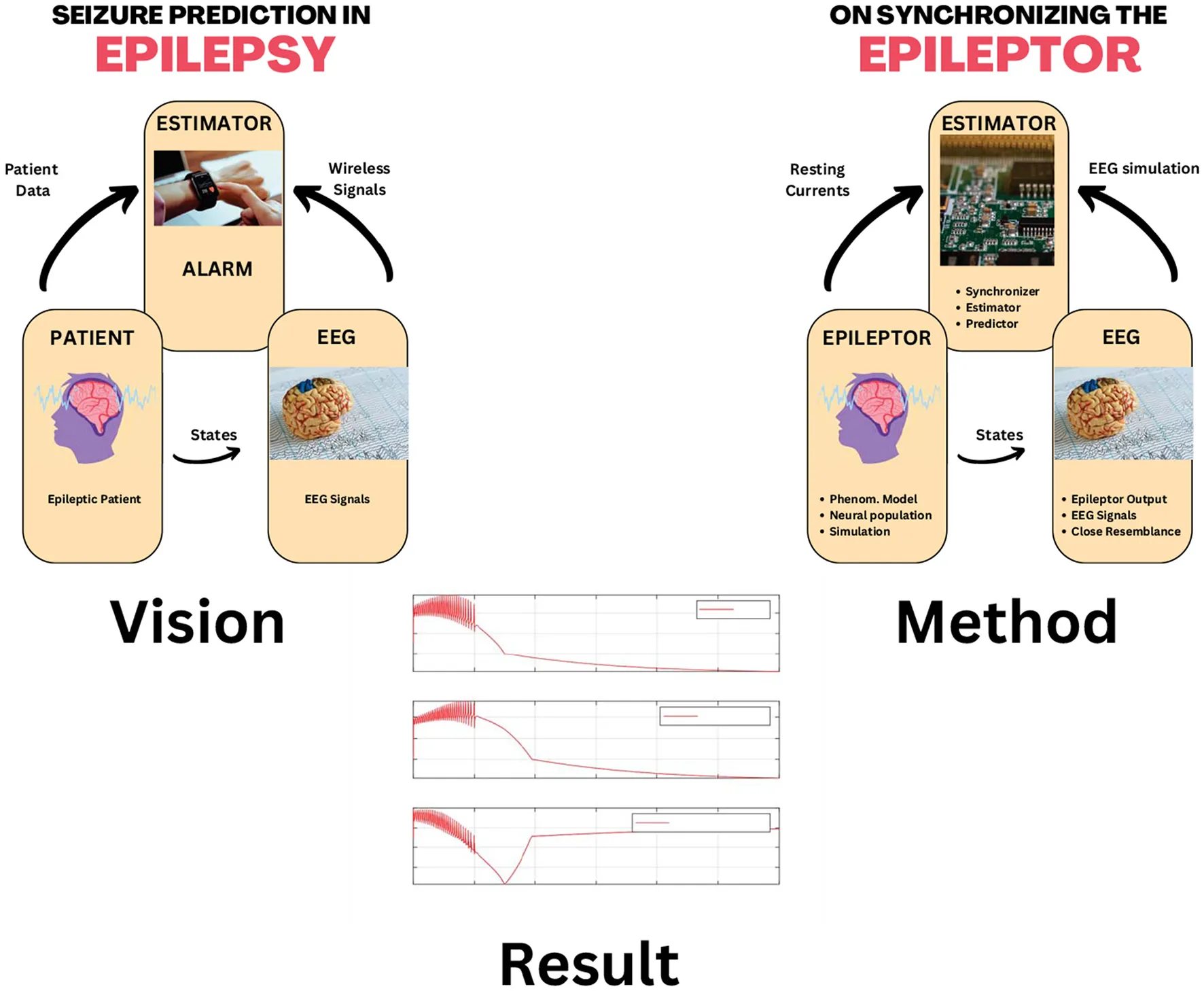
Epilepsy is one of the oldest known neural diseases in the history of mankind. It can be caused by a variety of malfunctions in the neural circuitry of the brain. It manifests itself in many forms, but it is mostly diagnosed by a characteristic signature in the patient's Electro-Encephalo-Gram (EEG). This signature is in the form of a typical train of pulses repeating at a very low but persistent frequency. In the non-linear systems parlance, one would be very much tempted to term it as the sign of a limit cycle, though one needs to go deeper to ascertain this conjecture. The human brain, consisting of networks of tens of billions of neurons, is a myriad of webs of non-linear dynamical systems interacting at several scales. These scales range from a non-linear dynamical system of a neuronal cell to complex feedback loops of neurons controlling several body functions, such as the cortico-thalamo-cortical loop (commonly called the ctc loop). This ctc loop is responsible for integrating sensory information into the decision-making neurons and connecting them back to the neurons controlling muscles. This is just one example from a multitude of feedback loops working on the neuronal network level in the human brain. The mentioned epileptic EEG signals (called eliptoform) may be caused by the gain/phase variations of the components of these feedback loops or even variations in the building block of these networks, such as a single neuron. A non-linear systems scientist may relate to the phenomenon of non-linear dynamical systems exhibiting characteristic oscillations, which are observed at particular instants of time when an otherwise healthy individual undergoes an epileptic episode, commonly called seizures. One is essentially looking at a non-linear dynamical system expressing markedly different responses, including oscillations of specific frequency. It is easy to relate such behavior to the phenomenon of bifurcation, i.e., a non-linear dynamic system showing markedly different behaviors upon the variations in its parameters. During an epileptic seizure, one may assume that certain parameters in the neurons in a particular neuronal network loop may undergo a change, resulting in the repeating pulse-like behavior. The exact dynamics of a seizure are certainly of interest, but the likelihood of having a seizure is a fundamental question haunting medical scientists and clinicians alike for decades. Life would be much easier for the epileptic patients if they knew the probability of getting a seizure while planning their daily activities or raising the level of precaution. One way to predict seizures may be to devise a pattern of the patient's behavior by relating bifurcation analysis to their EEG signals. These EEG signals are the measurement coming from the neuronal networks of the brain, with neurons as their building blocks. If one may observe the states of these neurons or a group of neurons by measuring EEG signals, and hence bifurcating patterns, in turn, seizures may be predicted. The context would be much clearer by consulting the graphical abstract in Figure 1. A well-established mathematical model may be synchronized with the EEG signal from a patient and the brain epilepsy states may be estimated and analyzed to predict epileptic seizure. This takes us to the problem of looking at the state estimators or the observers for the non-linear dynamic models of neurons. Interestingly, the idea of designing observers for the non-linear dynamic models of neurons is not new. Such efforts have been going on for many years. More than a decade ago, there was a surge in the efforts of observer design for neuronal models. Not knowing the cause of that trend, such observers could have been used for an attempt at seizure prediction, but the literature does not hint in this direction. Before commenting on the non-linear dynamic aspects of these designed observers, a certain biological fact emerges from the study of these observers. In a classical neuronal model, there are slow dynamics and fast dynamics [1, 2]. The fast dynamics are the Neuronal Output Voltage (coming from the Nernst Equation) and a state variable relating to the ion channel formations. The slow dynamics pertain to the ionic exchanges and distributions both inside and outside of a neuron cell. Most of the neuronal model observers seen in the literature need knowledge of the charge distribution, which may not be measured in real time at low cost. Estimation of the slow dynamics of a biological model may be a problem. However, the bifurcation analysis performed so far involves both fast and slow dynamics. Thus making a case for designing a neuronal observer that estimates both fast and slow states. It would also be of interest to look at the feasibility of such an observer from a non-linear observability standpoint. So far, we have motivated the need for a neuronal observer that may estimate and track a neuron cell and predict its states in real time to predict an epileptic seizure. It has been stressed in the literature that predicting slower dynamics is crucial, as they represent ionic exchange, which is the major cause or precursor to the triggering of fast dynamics of electric pulse train generation, which is the hallmark of a seizure. However, most of the neuronal observers designed so far either focus on the faster dynamics only or do not represent a biological model because of the problem of unknown biological parameters. For this reason, many of the designed observers are built on the basis of phenomenological models. Epileptor is such a phenomenological model which shows high fidelity to EEG data and also is amenable to non-linear analysis [3–5]. A vast body of studies exists on observer design for non-linear systems, but we will only review the studies related to the observer design for neuronal models. There are two main approaches: the Kalman Filter-based and the other using geometric control theory. In the Kalman Filter domain, all the varieties of Kalman Filter, like Extended Kalman Filter (EKF) and Unscented Kalman Filter (UKF), were proposed [6]. This design method has two main aspects that should be carefully analyzed. The model used by the Kalman Filter and its variants is essentially a linearized version of the neuron's non-linear dynamics around a particular equilibrium point, and if the equilibrium point shifts, the model will essentially change too, thus not helping in any seizure prediction based on bifurcation analysis. In addition, the underlying stochastic distributions are mostly assumed to be Gaussian or at least known, which is hardly the case. In the case of a neuron, both process and measurement uncertainty are not known a priori. The second approach looks ideal and promising.
Figure 1
In general control theory, a large body of study for non-linear observer design consists of Non-linear Lipschitz Observers, where a significant part of the model is linear, while the non-linear part comprises Lipschitz Non-linearity. If such a method is attempted on a Neuron model, then the linear part on its own does not remain observable, as the author attempted it for the unified neuron model proposed by depannenmacher [1, 7], and background given in Depannemaecker et al. [8, 9]. The non-linear observer design using geometric control theory was presented by Fairhust et al. [10]. They proposed such observers by using a second-order phenomenological model of a Neuron called the Rose and Hindmarsh model [11]. A formal framework for such design was presented by Astolfi [12]. Most of the geometric control theoretic approaches are centered on finding a diffeomorphism or non-linear transformation that may bring the neuronal model into a canonical non-linear observer form. As Astolfi mentioned himself, this step is not straightforward and may represent a major hurdle in the current pursuit. The onus is on the design of a non-linear observer utilizing the biological model of the neuron, and it should be capable of observing and hence estimating all the dynamics of the neuron, both faster (electrical) and slower ones (ionic flows). A novel breakthrough is required in the geometric theory of observer design. Another issue is nonlinear observability. Please see the study of Hermann [13], Isidori [14], and others [15, 16] for further details. Regarding biological models, a good starting point is the study of Huxley and Hodgkin (H-H model) [17], and a recent addition could be the study by the team of V. Jirsa [1]. It may be added that the task at hand is daunting but feasible. Sotomayor et al. [18] proposed an Extended Kalman Filter (EKF) to be used as an observer for Epileptor, which is a phenomenological model of a neuron. Since an EKF depends on a linearized model at every update, it is an approximation to the actual non-linear model at best. An observer is needed that may utilize the non-linear functions and structure of a neuron model, in this case, an Epileptor model. Brogin et al. [19–21] proposed an Epileptor observer by approximating the Epileptor model non-linearities with a bank of simplified Fuzzy membership functions. The approximation uses the differential mean value theorem, which may only be used for continuous functions.
There is a clear need for an observer design technique that may take into account the Epileptor non-linear model, per se, without any approximations. The Epileptor system is discontinuous, non-linear, and exhibits bifurcation. There is a wide body of studies dealing with the design of observers for systems with Lipschitz or monotonic non-linearities. These Linear matrix inequalities (LMI) based Observers, despite being linear in structure, can estimate the states of a system with Lipschitz non-linearities without any approximation. In the past, for such non-linear systems, the observers may be constructed using the Riccati Equation solution and later on by a convex optimization framework. Raghavan and Hedrick [22] and Rajamani [23] proposed linear observers for systems with Lipschitz non-linearities by posing the problem as a Riccati Equation. This was further improved upon by Phanomcheong and Rajamani in 2010 [24]. The problem with the Riccati solution is finding the right parameters so that the posed Riccati Equation is solvable or feasible. This problem was solved by the LMI-based convex optimization by Boyd [25] and the relevant software yalmip [26] to a larger extent. Arcak and researchers [27] posed an LMI observer for such systems. Arcak devised a method so that the structure of the model's non-linearity becomes a part of the observer, thus rendering the observer non-linear. Zemouche et al. used this concept in their LMI-based observer for the systems with Lipschitz non-linearities and later extended it to cover the systems with monotonic non-linearities [28]. They proposed a way to add further parameterization in the non-linearity structure so that the LMI problem can be solved more effectively.
This study addresses the design and simulation of an observer of a phenomenological model of an epileptic seizure using an LMI-based observer design for systems with Lipschitz non-linearity.
1.1 Aims of this study
This manuscript addresses three specific objectives:
To design a non-linear observer for the Epileptor model that preserves its discontinuous dynamics without resorting to linearization.
To formulate the observer design as a Linear Matrix Inequality (LMI) optimization problem that guarantees exponential convergence.
To demonstrate through simulation that estimated states can reliably track bifurcation parameters relevant for seizure prediction.
1.2 Main findings
Our key contributions are:
A Lipschitz observer design that handles discontinuous non-linearities (f1, f2) and monotonic function (g) without approximations.
LMI-based synthesis ensuring exponential convergence with rate α = 0.1.
Simulation validation with 50% initial condition mismatch tolerance.
Convergence within 5–10 seconds, providing sufficient prediction lead time.
Section two discusses the design methodology, and the results are discussed in Section three. Conclusions are drawn in the last section.
2 Methods
The section pertains to the description of the Epileptor model and the subsequent design of its observer based on the Lipschitz non-linear observer theory. The framework is symbolized in Figure 2.
Figure 2
2.1 Physical background and model justification
2.1.1 Neurophysiological background
Epileptic seizures arise from abnormal, excessive, and synchronous neuronal activity in the brain [29]. At the cellular level, seizures result from an imbalance between excitatory and inhibitory neurotransmission, leading to hyperexcitable neuronal populations. During the transition from the inter-ictal (between seizures) to the ictal (seizure) state, populations of neurons undergo a rapid shift in their firing patterns, manifesting as characteristic changes in electroencephalogram (EEG) recordings [30].
From a dynamical systems perspective, epileptic seizures can be understood as transitions between distinct attractors in the phase space of neural population activity [31]. The inter-ictal state corresponds to a stable fixed point or limit cycle representing normal brain activity. As system parameters slowly drift—due to ionic concentration changes, metabolic factors, or network reorganization—the system approaches a bifurcation point. Crossing this bifurcation threshold triggers a rapid transition to the ictal attractor, characterized by high-amplitude, rhythmic oscillations observable in EEG [3].
Understanding seizure generation as a bifurcation phenomenon provides a principled framework for prediction by monitoring the system's proximity to the bifurcation boundary; one can anticipate seizure onset before clinical manifestations appear [32].
2.1.2 Phenomenological modeling rationale
Neuronal models span a spectrum from detailed biophysical models to abstract phenomenological representations. Detailed models, such as the Hodgkin-Huxley formulation [17], capture ionic currents and membrane dynamics at the single-neuron level. While biophysically accurate, such models require extensive parameterization (dozens of variables per neuron) and are computationally prohibitive for real-time applications or population-level analysis [33].
Phenomenological models, by contrast, abstract the essential dynamical features without explicitly representing underlying ionic mechanisms. These models operate at the mesoscopic scale—capturing the collective behavior of neuronal populations rather than individual neurons—and are designed to reproduce key observable phenomena such as EEG waveforms, seizure onset dynamics, and bifurcation structure [34].
The trade-off is clear:
Biophysical models: High biological detail, but computationally expensive and require patient-specific physiological parameters that are difficult to measure clinically.
Phenomenological models: Computationally efficient, fewer parameters, and designed to match observable EEG dynamics, making them suitable for real-time state estimation and control applications.
For seizure prediction via state estimation, phenomenological models offer a practical advantage: they capture the bifurcation structure essential for prediction while remaining computationally tractable for observer design [35].
2.1.3 The epileptor model: justification and design principles
The Epileptor model was introduced by Jirsa et al. [3] as a generic phenomenological model capable of reproducing diverse seizure types observed clinically. The model's design is rooted in three key principles:
2.1.3.1 Two-timescale separation
The Epileptor employs a fast subsystem (variables x1, x2) representing rapid neuronal population dynamics observable in EEG, coupled to a slow subsystem (variable z) that modulates the bifurcation structure. This separation mirrors the clinical observation that seizures involve both fast oscillatory activity (ictal discharges) and slow processes (pre-ictal buildup, post-ictal depression) [36].
2.1.3.2 Bifurcation-based seizure mechanism
The model is constructed such that seizure onset occurs via a saddle-node bifurcation, a well-established mechanism in neural population models [37]. The bifurcation parameter x0 controls the threshold for seizure initiation. As the slow variable z evolves, it modulates x0, causing the system to cross the bifurcation boundary and trigger a seizure.
2.1.3.3 Discontinuous dynamics
The Epileptor incorporates piecewise-defined functions f1 and f2 that switch at x1 = 0, representing qualitatively different dynamics in inter-ictal vs. ictal states. While this introduces mathematical complexity (discontinuous right-hand side), it enables accurate reproduction of the abrupt transitions observed in clinical EEG [3].
2.1.3.4 Validation against clinical data
The Epileptor has been extensively validated against human EEG recordings from patients with focal epilepsy. The model successfully reproduces:
Temporal patterns of seizure onset and termination.
Spectral characteristics of ictal discharges.
Inter-seizure interval variability.
Response to parameter perturbations mimicking antiepileptic drugs.
These validations establish the Epileptor as a clinically relevant model for seizure dynamics [5, 38].
2.1.4 Main assumptions
The Epileptor model, as used in this study, relies on the following assumptions:
Single epileptogenic zone: The model represents a single focal region. Extension to multi-focal epilepsy requires coupled Epileptor networks [39].
Phenomenological parameter sufficiency: The model's parameters (x0, τ0, Irest1, etc.) are assumed to capture the effective dynamics of the underlying neuronal population without requiring detailed ionic or synaptic parameters.
EEG approximates x1: The fast variable x1 is assumed to be directly observable (or closely approximated) by scalp or intracranial EEG recordings. This is justified by the model's design, where x1 represents the dominant oscillatory mode [3].
Bifurcation parameter determines seizure threshold: The parameter x0 is assumed to encode the proximity to seizure onset. Estimating x0 (or its time-varying drift) enables the prediction of bifurcation crossing.
Quasi-static slow dynamics: The ultra-slow variable y evolves on timescales much longer than seizure duration, justifying its treatment as a slowly varying parameter during individual seizure cycles.
2.1.5 Model advantages
The Epileptor model offers several advantages for observer-based seizure prediction:
Computational efficiency: With only 5 state variables, the model is suitable for real-time simulation and observer implementation on embedded hardware [35].
Clear dynamical interpretation: Each variable and parameter has a well-defined role in the bifurcation structure, facilitating interpretation of estimated states in terms of seizure risk.
Diverse seizure reproduction: The model can generate various seizure patterns (tonic, clonic, tonic-clonic) by adjusting parameters, providing flexibility for patient-specific tuning [3].
Observer design compatibility: Despite discontinuities, the model's non-linearities are of Lipschitz and monotonic class, enabling rigorous observer synthesis via LMI methods [23, 40].
Established validation: Extensive prior study has validated the model against clinical data, providing confidence in its predictive utility [38].
2.1.6 Model limitations
While powerful, the Epileptor has inherent limitations:
Phenomenological abstraction: The model does not capture detailed ionic mechanisms (sodium, potassium, and calcium currents) or specific neurotransmitter dynamics. Mechanistic insights are therefore limited.
Focal seizure specificity: The model is best suited for focal (partial) seizures with clear pre-ictal buildup. Generalized seizures (absence, myoclonic) may require alternative formulations [41].
Parameter personalization required: The model's parameters must be tuned to individual patients. Generic parameters may not accurately predict seizure timing for a specific patient.
Single-region assumption: The basic Epileptor represents a single epileptogenic zone. Multi-focal epilepsy or seizure propagation through networks requires coupled Epileptor models, increasing complexity.
Discontinuity challenges: The piecewise-defined functions complicate mathematical analysis (existence, uniqueness, and observability) and require careful numerical treatment [18].
Despite these limitations, the Epileptor remains one of the most widely used phenomenological models for computational epilepsy research, balancing biological realism with mathematical tractability [42].
2.2 The Epileptor model
2.2.1 Model variables and parameters
The Epileptor model describes the dynamics of a neuronal population through five state variables, each representing distinct temporal and functional aspects of seizure generation. Table 1 provides a complete specification of all variables, their units, and physical interpretation.
Table 1
| Variable | Description | Units | Physical meaning |
|---|---|---|---|
| x1 | Fast population activity | mV | Membrane potential of pyramidal cells (EEG-observable) |
| x2 | Fast recovery variable | mV | Inhibitory population activity |
| z | Slow permittivity variable | Dimensionless | Slow modulation of excitability |
| y | Ultra-slow variable | Dimensionless | Very slow metabolic/homeostatic processes |
| u | Input current | pA | External stimulation or baseline drive |
Epileptor model variables and units.
The model parameters control the dynamical regime and bifurcation structure. Table 2 lists all parameters with their standard values and physical interpretation.
Table 2
| Parameter | Value | Units | Physical meaning |
|---|---|---|---|
| τ0 | 2,857 | ms | Time scale separation factor between fast and slow subsystems |
| τ2 | 10 | ms | Time constant of the fast subsystem |
| x0 | −2.2 to −1.6 | Dimensionless | Bifurcation parameter controlling seizure threshold |
| Irest1 | 3.1 | pA | Resting current for fast subsystem |
| Irest2 | 0.45 | pA | Resting current for slow subsystem |
| γ | 0.01 | Dimensionless | Coupling strength between subsystems |
Epileptor model parameters.
2.3 Model equations
The Epileptor dynamics are governed by the following system of ordinary differential equations:
The output equation, representing the EEG measurement, is:
2.3.1 Nonlinear functions: physical interpretation
The Epileptor's rich dynamics arise from three non-linear functions: f1, f2, and g. Each function is carefully designed to capture specific aspects of seizure generation and termination.
2.3.2 Function f1(x1, x2, z): fast subsystem dynamics
The function f1 is piecewise-defined:
2.3.2.1 Physical meaning
Cubic nonlinearity (x1 < 0): This term provides the saddle-node bifurcation structure essential for seizure onset. The cubic polynomial has a local maximum and minimum, creating a bistable regime. When the system is driven past the saddle point, it rapidly transitions to the ictal state.
Parabolic modulation (x1 ≥ 0): The term shows how the slow variable z modulates the bifurcation point. As z evolves, it shifts the effective bifurcation parameter, causing the system to approach and cross the seizure threshold. The parabolic dependence on z creates a smooth modulation of excitability.
Discontinuity at x1 = 0: This switching surface represents a qualitative change in dynamics between inter-ictal (negative x1) and ictal (positive x1) states. The discontinuity captures the abrupt nature of seizure onset observed clinically.
2.3.3 Function f2(x1, x2): recovery dynamics
The function f2 governs the recovery variable x2:
2.3.3.1 Physical meaning
State-dependent recovery: The piecewise structure reflects different recovery mechanisms in inter-ictal versus ictal states. During inter-ictal periods (x1 < 0), recovery is slow and depends on the permittivity variable z. During seizures (x1 ≥ 0), recovery is faster and proportional to the amplitude of x1.
Quintic term (x1 < 0): The term 0.6(z − 4)5 provides a strong restoring force that terminates seizures. The fifth-power dependence creates a sharp increase in inhibitory drive as z deviates from its resting value, ensuring seizure termination.
Linear coupling (x1 ≥ 0): During ictal states, the term 6(x1 − 0.25) couples recovery directly to population activity, representing activity-dependent inhibition (e.g., GABAergic feedback).
2.3.4 Function g(x1): sigmoid integration
The function g is defined as an integral of a sigmoid:
2.3.4.1 Physical meaning
Smooth threshold function: The sigmoid 1/(1 + e−10(ξ+0.25)) represents a smooth activation threshold. It is approximately zero for ξ < −0.25 and approaches 1 for ξ > −0.25, capturing the notion of a firing threshold in neuronal populations.
Monotonic increasing: Since the integrand is always non-negative, g(x1) is strictly increasing. This monotonicity is crucial for observer design, as it ensures that the coupling term γg(x1) in Equation 4 has well-defined Lipschitz properties.
Biological interpretation: The function g can be interpreted as modeling cumulative excitation or calcium-dependent processes that evolve on slower timescales. The integral form smooths rapid fluctuations in x1, providing a low-pass filtered signal to the ultra-slow variable y.
2.3.5 Why these specific functions?
The choice of f1, f2, and g is not arbitrary but carefully motivated by several considerations:
Bifurcation structure: The cubic non-linearity in f1 is the minimal polynomial required to produce a saddle-node bifurcation, which is the canonical mechanism for seizure onset in neural population models [37].
Time-scale separation: The piecewise structure and the slow modulation via z enable the model to exhibit distinct inter-ictal, pre-ictal, ictal, and post-ictal phases, matching clinical observations [42].
Computational tractability: Despite their complexity, these functions are piecewise polynomial or involve standard functions (exponentials, integrals), making them computationally efficient to evaluate and differentiate—essential for real-time observer implementation.
Validation against data: The specific functional forms and parameter values were calibrated by Jirsa et al. [42] to reproduce the temporal and spectral characteristics of human EEG recordings from patients with temporal lobe epilepsy. Subsequent studies have confirmed the model's ability to capture diverse seizure patterns [5, 39].
Observer design compatibility: The functions f1 and f2, while discontinuous, satisfy local Lipschitz conditions in each region (x1 < 0 and x1 ≥ 0). The function g is smooth and monotonic. These properties enable the application of Lipschitz observer design techniques [23, 43], which is the foundation of our approach.
2.3.6 Dynamical behavior and seizure mechanism
To understand how the Epileptor generates seizures, consider the interaction between fast and slow variables:
2.3.6.1 Inter-ictal state (x1 < 0)
In this regime, the system resides in a stable fixed point corresponding to normal brain activity. The slow variable z gradually evolves according to Equation 3, approaching the value z ≈ 4(x1 − x0).
2.3.6.2 Pre-ictal transition
As z increases (due to the dynamics of Equation 3), the effective bifurcation parameter in f1 shifts. When z crosses a critical threshold, the stable fixed point in the x1 < 0 region disappears via a saddle-node bifurcation. The system is then forced to transition to the x1 ≥ 0 region.
2.3.6.3 Ictal state (x1 ≥ 0)
Once x1 becomes positive, the dynamics switch to the second branch of f1 and f2. The system exhibits large-amplitude oscillations, corresponding to the high-frequency, high-amplitude EEG activity characteristic of seizures.
2.3.6.4 Seizure termination
The quintic term in f2 provides a strong inhibitory drive that eventually suppresses the oscillations. Simultaneously, the slow variable z decreases (due to the negative feedback in Equation 3), restoring the bifurcation structure to favor the inter-ictal state. The system transitions back to x1 < 0, ending the seizure.
This bifurcation-based mechanism is consistent with the theory of dynamical diseases [44] and has been validated against clinical data [42].
2.4 Epileptor model adaptation for observer design
The non-linear functions in the epileptor model are discontinuous in the model state space. As these discontinuities are on x1 = 0 and x2 = −0.25. So these thresholds mark the boundaries dividing the state space into four quadrants, each quadrant following its own sub-model. The four quadrants have these four sub-models, which are explained below:
Quadrant I, x1 ≥ 0, x2 ≥ −0.25.
Quadrant II, x1 < 0, x2 ≥ −0.25.
Quadrant III, x1 < 0, x2 ≤ 0.25.
Quadrant IV, x1 ≥ 0, x2 < −0.25.
The detailed respective sub-models are given in the Appendix. The sub-model of Quadrant I is given as:
For Quadrant II:
For Quadrant III:
For Quadrant IV:
Where A1 is the system matrix prevalent in Quadrant I, γ1 is the state non-linear function relevant to Quadrant I, and η1 is the vector containing external signals and biases. Regarding the states x1 and x2 are coming directly from the EEG measurement with your units in mill-volts or micro-volts. The output y is defined as:
where C = [−1 0 0 1 0]. Time lags, or constants, are incorporated through the states y1, y2, and z. So these time constants express themselves in the pivotal or diagonal elements of the system matrix A1. These constants also find their way in the bias term η1. The second set of constants is external signals Irest1 and Irest2. These are important to mention as the nominal values are suggested in Jirsa et al. [3], Saggio and Jirsa [45], and Saggio et al. [46], but they may change considerably in the actual situations. Similarly, the equilibrium or setpoints x0 and y0 may also change. For the LMI-based observer design, one may assume the Linear Parameter Varying (LPV) approach, where the vertices of the state space of interest are identified, and for each of the vertex models, an observer is designed. For the observer implementation, all of the designed observers are then incorporated in an LPV manner. To make the resulting observer easy to implement in real-time, only one observer is designed based on the worst-case scenario. Keeping this in mind, Quadrant I seems appropriate. As per the above discussion, the LMI observer for the Lipschitz non-linear system of Quadrant I is designed in the next Section.
2.5 Mathematical analysis: well-posedness of the epileptor model
2.5.1 Challenge of discontinuous right-hand side
The Epileptor model, as defined by Equations 1–5, presents a mathematical challenge: the functions f1(x1, x2, z) and f2(x1, x2) are discontinuous at x1 = 0. This discontinuity violates the standard assumptions of classical existence and uniqueness theorems for ordinary differential equations.
Specifically, the Picard-Lindelöf theorem requires that the right-hand side of the ODE system be Lipschitz continuous in the state variables. However, the piecewise definition of f1 and f2 creates a jump discontinuity at the switching surface .
Without establishing well-posedness, the following questions remain unanswered:
Do solutions exist for all initial conditions?
Are solutions unique?
How should solutions be interpreted when the trajectory crosses x1 = 0?
Can numerical simulations be trusted to represent true system behavior?
These questions are not merely academic; they are essential for justifying observer design and ensuring that state estimation algorithms converge to physically meaningful trajectories.
2.5.2 Filippov solution framework
To rigorously address discontinuous differential equations, we adopt the framework developed by Filippov [47]. This theory extends the notion of solutions to systems with discontinuous right-hand sides by introducing set-valued maps and convex combinations of vector fields.
2.5.3 Filippov set-valued map
Consider a general system of the form:
where f:ℝn → ℝn is piecewise continuous but may have discontinuities on a surface Σ.
2.5.3.1 Definition (Filippov set-valued map)
The Filippov set-valued map is defined as:
where:
B(x, δ) is a ball of radius δ centered at x,
μ(S) = 0 denotes sets S of Lebesgue measure zero,
co{·} denotes the convex hull.
Intuitively, is the smallest convex set containing all limit points of f as one approaches x from any direction, excluding sets of measure zero (e.g., the discontinuity surface itself).
2.5.3.2 Definition (Filippov solution)
An absolutely continuous function x : [0, T] → ℝn is a Filippov solution of Equation 26 if:
This definition allows solutions to “slide” along discontinuity surfaces by taking convex combinations of the vector fields on either side of the surface.
2.5.4 Well-posedness of the epileptor
We now establish the existence and uniqueness of Filippov solutions for the Epileptor model.
2.5.5 Theorem 1: existence and uniqueness
[Well-posedness of the epileptor model]
For any initial condition , the Epileptor system (Equations 1–5) admits a unique Filippov solution x(t) = (x1(t), x2(t), z(t), y(t), u(t)) defined for all t ∈ [0, T], for any T > 0.
2.5.6 Proof sketch
The proof proceeds in four steps:
2.5.6.1 Step 1: boundedness of solutions
We first show that solutions remain bounded on finite time intervals. The non-linear terms f1 and f2 grow at most polynomially (cubic and quintic, respectively). The equations for z, y, and u are linear or involve bounded non-linearities. By constructing a Lyapunov-like function:
one can show that is bounded by a quadratic function of V, implying:
for some constant C > 0. Thus, solutions cannot escape to infinity in finite time.
2.5.6.2 Step 2: one-sided lipschitz property
Away from the switching surface Σ = {x1 = 0}, the functions f1 and f2 are smooth (polynomial). In each region {x1 < 0} and {x1 > 0}, the right-hand side satisfies a local Lipschitz condition. Specifically, for any compact set K⊂{x1 < 0} or K⊂{x1 > 0}, there exists a Lipschitz constant LK such that:
Moreover, even at the discontinuity, the system satisfies a one-sided Lipschitz condition:
for some constant LOSL. This property ensures that trajectories do not exhibit “Zeno behavior” (infinitely many crossings in finite time).
2.5.6.3 Step 3: Filippov convexification at the switching surface
At points on the switching surface Σ = {x1 = 0}, the Filippov set-valued map is the convex hull of the limits from the left () and right (). Explicitly:
For the Epileptor, the limits are:
and similarly for f2. The convex hull is a line segment connecting these two values, ensuring that is upper semicontinuous.
By the Filippov existence theorem [47], upper semicontinuity of and boundedness of solutions guarantee the existence of at least one Filippov solution.
2.5.6.4 Step 4: uniqueness via transversal crossing
To establish uniqueness, we show that the switching surface Σ is non-attractive, meaning that trajectories cross Σ transversally rather than sliding along it indefinitely.
Consider the dynamics of x1 near x1 = 0:
At x1 = 0:
If y − u > 0, then ẋ1 > 0, and the trajectory crosses from x1 < 0 to x1 > 0.
If y − u < 0, then ẋ1 < 0, and the trajectory crosses from x1 > 0 to x1 < 0.
If y − u = 0, the trajectory is tangent to Σ, but this is a measure-zero event.
Since y and u evolve according to smooth dynamics (Equations 4, 5), the condition y − u = 0 is generically non-persistent. Thus, trajectories cross Σ transversally, and uniqueness follows from the standard Filippov uniqueness theorem [47].
2.5.7 Rigorous proof
A complete, rigorous proof with detailed technical lemmas is provided in Appendix A. The proof relies on the following key results from the theory of differential equations with discontinuous right-hand sides:
Filippov existence theorem: If is upper semicontinuous and locally bounded, then Filippov solutions exist [47].
Filippov uniqueness theorem: If the switching surface is non-attractive (transversal crossing), then Filippov solutions are unique [48].
One-sided Lipschitz theory: Systems satisfying one-sided Lipschitz conditions admit unique solutions even with discontinuities [15].
2.6 Implications for observer design
The well-posedness of the Epileptor model has several important implications for our observer design:
2.6.1 Well-defined state trajectories
Theorem 1 in Section 2.5.5 guarantees that the Epileptor generates unique, physically meaningful trajectories for any initial condition. This ensures that the “true state” x(t) exists and is uniquely determined by the initial condition and model parameters. The observer's goal—to estimate x(t) from measurements—is therefore well-defined.
2.6.2 Observer convergence
The Filippov framework justifies treating the discontinuities in f1 and f2 as bounded perturbations when designing the observer. Specifically, the Lipschitz observer design (Section 3) relies on bounding the non-linearities by Lipschitz constants. In each region (x1 < 0 and x1 ≥ 0), the system is locally Lipschitz, and the observer can be designed separately for each region (quadrant-based design). The transversal crossing property ensures that the observer does not encounter pathological behavior at the switching surface.
2.6.3 Numerical implementation
The existence and uniqueness of Filippov solutions justify the use of standard ODE solvers (e.g., Runge-Kutta methods) with appropriate step size control. At the switching surface x1 = 0, the solver should reduce the step size to accurately detect the crossing. The Filippov theory guarantees that the numerical solution converges to the true Filippov solution as the step size decreases.
2.6.4 Observability analysis
Well-posedness is a prerequisite for observability analysis. Since solutions are unique, the output trajectory y(t) = x1(t) − x2(t) is uniquely determined by the initial state. Observability then concerns whether different initial states produce distinguishable output trajectories. The Filippov framework ensures that observability analysis is mathematically sound [15].
In summary, the Filippov solution framework provides a rigorous foundation for our observer design, ensuring that the estimated states converge to the true (unique) system trajectory despite the presence of discontinuities.
2.7 Quadrant invariance and boundary dynamics
The quadrant-based observer design relies on partitioning the (x1, x2) phase plane into four regions, each corresponding to a distinct phase of seizure dynamics. In this subsection, we rigorously analyze the dynamical behavior at quadrant boundaries and establish that these regions are meaningful for observer design.
2.7.1 Quadrant definitions
We partition the (x1, x2) phase plane into four quadrants:
The boundaries between quadrants are:
2.7.2 Proposition 1: quadrant forward invariance and boundary crossing
[Quadrant dynamics] For the Epileptor fast subsystem (Equations 1, 2), the quadrants Q1, Q2, Q3, Q4 are dynamically meaningful regions in the following sense:
Trajectories cross quadrant boundaries in well-defined directions corresponding to seizure state transitions.
The boundaries and are non-attractive, meaning that trajectories cross transversally rather than sliding along the boundaries indefinitely.
Each quadrant corresponds to a distinct phase of the seizure cycle: inter-ictal (Q3), pre-ictal (Q2), ictal (Q1), and post-ictal (Q4).
2.7.3 Proof
We analyze the vector field at each boundary to determine the direction of crossing.
2.7.3.1 Boundary : {x1 = 0}
At the vertical boundary x1 = 0, the dynamics of x1 are governed by:
We consider two cases:
Case 1: Approaching from x1 → 0− (from Q2 or Q3):
Using the definition of f1 for x1 < 0:
Thus:
If y − u > 0 (which occurs during the pre-ictal buildup when y increases), then ẋ1 > 0. The trajectory crosses from Q2 to Q1, corresponding to seizure onset.
If y − u < 0, then ẋ1 < 0, and the trajectory remains in or returns to Q2 or Q3.
Case 2: Approaching from x1 → 0+ (from Q1 or Q4):
Using the definition of f1 for x1 ≥ 0:
Thus:
During seizure termination, y decreases (becomes negative) and x2 is typically positive. If y + x2 − u < 0, then ẋ1 < 0. The trajectory crosses from Q1 to Q2, corresponding to seizure offset.
If y + x2 − u > 0, the trajectory remains in Q1 (ongoing seizure).
Conclusion for: The boundary is crossed in directions determined by the sign of y − u (from the left) or y + x2 − u (from the right). These crossings are transversal (not tangent), and the direction corresponds to the clinical interpretation: Q2 → Q1 is seizure onset, and Q1 → Q2 is seizure termination.
2.7.3.2 Boundary : {x2 = −0.25}
At the horizontal boundary x2 = −0.25, the dynamics of x2 are governed by:
We consider two cases based on the sign of x1:
Case 1: x1 < 0 (in Q2 or Q3):
Using the definition of f2 for x1 < 0:
Thus:
With Irest1 = 3.1 and z ≈ 4 (near equilibrium), we have:
Therefore, trajectories move upward (increasing x2) when approaching x2 = −0.25 from below. This means:
Trajectories in Q3 cross into Q2 (transition from deep inter-ictal to pre-ictal).
Trajectories in Q2 do not cross into Q3 unless perturbed.
Case 2: x1 ≥ 0 (in Q1 or Q4):
Using the definition of f2 for x1 ≥ 0:
Thus:
If x1 < 0.725, then ẋ2 > 0, and the trajectory moves upward (from Q4 to Q1).
If x1 > 0.725, then ẋ2 < 0, and the trajectory moves downward (from Q1 to Q4, post-ictal phase).
Conclusion for: The boundary is also crossed transversally. The direction depends on the value of x1:
For x1 < 0 (inter-ictal), trajectories move upward (Q3 → Q2).
For small x1 ≥ 0 (early ictal), trajectories move upward (Q4 → Q1).
For large x1 ≥ 0 (late ictal), trajectories move downward (Q1 → Q4, post-ictal recovery).
2.7.4 Interpretation: quadrants as dynamically meaningful regions
The analysis above shows that the quadrants Q1, Q2, Q3, Q4 are not strictly invariant (trajectories do cross boundaries), but the crossing directions are well-defined and correspond to seizure state transitions:
Q3(Inter-ictal): Deep resting state, x1 < 0, x2 < −0.25. Trajectories slowly evolve toward Q2 as z increases.
Q2(Pre-ictal): Buildup phase, x1 < 0, x2 ≥ −0.25. As y increases, the system approaches the boundary x1 = 0 and prepares to cross into Q1.
Q1(Ictal): Seizure state, x1 ≥ 0, x2 ≥ −0.25. Large-amplitude oscillations occur. The system eventually transitions to Q4 or back to Q2 as y decreases.
Q4(Post-ictal): Recovery phase, x1 ≥ 0, x2 < −0.25. The system transitions back to Q3 or Q2 as x1 decreases.
2.7.5 Implications for observer design
The quadrant structure has important implications for observer design:
Lipschitz constants: In each quadrant, the functions f1 and f2 are smooth (polynomial), and different Lipschitz constants apply. The observer gain can be optimized separately for each quadrant, improving convergence rates.
Bifurcation parameter tracking: The transition from Q2 to Q1 (seizure onset) is the critical event for prediction. By monitoring the estimated state's proximity to the boundary , the observer can provide advance warning of seizure onset.
Clinical interpretation: Each quadrant corresponds to a clinically recognizable seizure phase. The observer's estimated quadrant can be displayed to clinicians, providing intuitive information about seizure risk.
Switching observer design: The transversal crossing property justifies a switching observer design, where the observer switches between different gain matrices as the estimated state crosses quadrant boundaries. The Filippov framework (Section 2.3) ensures that this switching is well-defined and does not introduce spurious oscillations.
In summary, the quadrant structure is not merely a mathematical convenience but reflects the underlying dynamical organization of the Epileptor model. The boundaries correspond to bifurcation-like transitions between seizure phases, and the transversal crossing property ensures that observer design is mathematically sound.
2.8 Observer design for Epileptor
The Observer for the epileptor is designed using the methodology proposed by Zemouche et al. [28, 40, 43]. If the system is given as:
where n is the number of states, m is the number of non-linear functions such that : x ϵ Rn are the epileptor states, γ ϵ Rm is the vector of the non-linear functions γ1 γ2..γm in the epileptor model,
and ω ϵ Rq is the disturbance. The matrix A ϵ Rn×n is the system matrix, G ϵ Rn×m is the distribution matrix for the non-linear functions, and E ϵ Rn×q is the disturbance distribution matrix. Both D and E are taken to be null as the disturbance is assumed to be absent. In the case of the epileptor model, it is to be noted that out of the six epileptor states, only a few of them are used by each non-linear function γi(x). From the epileptor model of Quadrant I (Equation 11) the nonlinearities are :
Rewriting the nonlinear functions γi(x) as γi(Hix).
where
if n1 is the number of state variables used in γ1(x), then . Similarly:
The non-linearity function distribution matrix G for the Epileptor Quadrant 1 model is formulated as:
First state is acted upon by γ1(x), the second state by γ2(x) and the fourth state by γ3(x). In the last, the application of Lipschitz constants is facilitated by the matrix :
where e(i) ϵ Rn is a vector with all elements to be zero except for the ith entry, which is made equal to 1. This is defined in Lemma 7 of Zemouche and Boutayeb [43]. The proposed observer structure is:
where:
The gain matrices to be designed are L, K1, K2, K3. These are designed by solving the following LMIs:
The next section discusses the issues of parameter tuning and observer convergence.
2.9 Numerical implementation
This section provides a detailed description of the numerical methods used to simulate the Epileptor model and the observer dynamics. Reproducibility is a cornerstone of scientific research; therefore, we specify all algorithms, parameters, and software tools employed in this study.
2.10 ODE solver selection
2.10.1 Epileptor model simulation
The Epileptor model (Equations 1–5) is a stiff system with multiple timescales and discontinuous right-hand side. We employ the following numerical strategy:
2.10.1.1 Method
4th-order Runge-Kutta (RK4) method with adaptive step size control.
2.10.1.2 Rationale
Accuracy: RK4 provides fourth-order accuracy, which is sufficient for capturing the fast oscillations during seizures while remaining computationally efficient.
Stiffness handling: While RK4 is not specifically designed for stiff systems, the adaptive step size control allows the solver to reduce the step size during rapid transitions (e.g., seizure onset), ensuring stability.
Discontinuity handling: At the switching surface x1 = 0, the step size is automatically reduced to detect the crossing accurately. The Filippov framework (Section 2.3) guarantees that the numerical solution converges to the true Filippov solution as the step size decreases.
2.10.1.3 Step size control
Initial step size: Δt0 = 0.1 ms.
Adaptive range: Δt ∈ [0.01, 1.0] ms.
Error tolerance: Local truncation error ϵ < 10−6.
Discontinuity detection: When |x1| < 0.01, the step size is reduced to Δtmin = 0.01 ms to ensure accurate crossing of the switching surface.
2.10.1.4 Implementation
The RK4 method with adaptive stepping is implemented in MATLAB using the ode45 solver with custom event detection for the switching surface. The event function monitors x1 and triggers a step size reduction when x1 approaches zero.
2.10.2 Observer dynamics simulation
The observer dynamics are integrated using the same RK4 solver to ensure consistency with the model simulation.
2.10.2.1 Synchronization
The observer and model are integrated with identical time steps. At each time step tk, the measurement yk = x1(tk)−x2(tk) is passed to the observer, and the observer state is updated. This synchronous integration mimics the continuous-time observer in discrete time.
2.10.2.2 Initial conditions
To test the observer's robustness, we initialize the observer with a 50% error relative to the true initial state:
This large initial mismatch simulates the realistic scenario where the observer starts with poor knowledge of the true state.
2.10.3 LMI solver for observer gain computation
The observer gain matrix L is computed offline by solving the Linear Matrix Inequality (LMI) conditions derived in Section 3.2. The LMI problem is formulated as:
where P is a symmetric positive-definite matrix, L is the observer gain, α > 0 is the desired convergence rate, θ > 0 is a tuning parameter, and Lf is the Lipschitz constant of the non-linear functions f1 and f2.
2.10.4 Software and solver configuration
2.10.4.1 Software
YALMIP toolbox [26] for MATLAB.
2.10.4.2 Rationale
YALMIP: A high-level modeling language for optimization problems, allowing intuitive specification of LMI constraints.
2.10.4.3 Solver settings
Tolerance: Primal and dual feasibility tolerance .
Optimality tolerance: Gap tolerance .
Maximum iterations: 1,000.
Feasibility check: After solving, we verify that P≻0 by checking that all eigenvalues of P are positive: λmin(P) > 0.
2.10.4.4 Implementation
The LMI problem is specified in YALMIP syntax as follows:
  % Define decision variables
  P = sdpvar(5, 5);  % Symmetric
   positive-definite matrix
  L = sdpvar(5, 1);  % Observer gain vector

  % LMI constraints
  Constraints = [P >= 1e-6 * eye(5)];
  % Positive definiteness
  Constraints = [Constraints, ...
      P*(A - L*C) + (A - L*C)'*P + alpha*P + ...
      theta^(-1)*P*E*E'*P + theta*Lf^2*eye(5)  < =
      -1e-6*eye(5)];

  % Solve
  options = sdpsettings('solver', 'mosek',
  'verbose', 1);
  sol = optimize(Constraints, [], options);

  % Extract solution
  P_opt = value(P);
  L_opt = value(L);
2.10.5 Computation time
The LMI problem is solved offline (once for each quadrant) before running the observer. Typical computation times on a standard workstation (Intel Core i7, 16 GB RAM) are:
LMI solution time: ~0.8 seconds per quadrant.
Total offline computation: ~3.2 seconds (4 quadrants).
This one-time offline computation is negligible compared to the online observer execution time.
2.10.6 Simulation parameters
Table 3 summarizes all numerical parameters used in the simulations.
Table 3
| Parameter | Value | Description |
|---|---|---|
| Simulation time | 300 s | Total duration, including multiple seizure cycles |
| Sampling rate (internal) | 10,000 Hz | Oversampling for accurate dynamics capture |
| Output sampling rate | 256 Hz | Matches clinical EEG sampling frequency |
| Measurement noise | σ = 0.01 mV | Additive Gaussian white noise on y = x1 − x2 |
| Initial error | 50% | Observer initialized at |
| Convergence rate | α = 0.1 | Desired exponential decay rate for observer error |
| Lipschitz constant | Lf = 10 | Conservative bound for f1 and f2 in each quadrant |
| Tuning parameter | θ = 0.1 | Balances non-linearity compensation in LMI |
Simulation configuration parameters.
2.10.7 Computational requirements
2.10.7.1 Hardware platform
Processor: Intel Core i7-10700K @ 3.8 GHz.
RAM: 16 GB DDR4.
Operating System: Windows 10 Pro.
Software: MATLAB R2023b.
2.10.7.2 Computation time
300 s simulation (Epileptor+Observer): ~2.5 seconds wall-clock time.
Speedup factor: 300/2.5 = 120 × real-time.
LMI solution (offline): ~0.8 seconds per quadrant.
2.10.7.3 Real-time feasibility
The computation time is significantly less than the simulation time, indicating that the observer can be implemented in real-time on standard hardware. For clinical applications, the observer could be deployed on embedded systems (e.g., FPGA, ARM Cortex) with modest computational resources.
2.10.7.4 Memory requirements
State storage: 5 × 2 = 10 double-precision variables (model + observer states).
Observer gain storage: 5 × 4 = 20 double-precision variables (one gain matrix per quadrant).
Total memory: < 1 KB, easily accommodated on embedded platforms.
2.10.8 Code availability
To promote reproducibility and facilitate future research, we provide the complete MATLAB implementation of:
Epileptor model simulation (including discontinuity handling).
LMI-based observer design (YALMIP).
Observer simulation and state estimation.
Visualization scripts for generating all figures in this manuscript.
2.10.8.1 Repository
The code will be made publicly available upon acceptance of this manuscript at:
The repository includes:
Documented MATLAB scripts.
Parameter configuration files.
Example datasets.
README with installation and usage instructions.
2.10.9 Numerical stability and verification
To ensure the correctness and stability of the numerical implementation, we perform the following verification steps:
2.10.10 Summary
This section has provided a comprehensive description of the numerical methods used in this study, including:
ODE solver selection and configuration (RK4 with adaptive stepping).
LMI solver setup (YALMIP).
Simulation parameters (Table 3).
Computational requirements and real-time feasibility.
Code availability and reproducibility.
Numerical stability verification procedures.
These details enable other researchers to reproduce our results and extend the methodology to related problems in computational neuroscience and epilepsy research.
3 Results and discussion
From Figures 3–5 it can be seen that the estimates of states x1 and x2 converge within 10 min, and the third state z takes more time to converge, even in excess of an hour. This excess time can be attributed largely to the two factors. The first is the large mismatch in the initial conditions of the epileptor and those of its observer, which amounts to nearly 20 percent of the final value of z. This mismatch is deliberately introduced to demonstrate its damaging effect. It can be assumed that in lab or clinic conditions, this observer will be allowed to run for a while under the healthy condition of the patient so that the epileptor observer converges to the actual value of z of the patient. It is worth noting that if the discussed initial condition mismatch is small enough, then the observer is shown to readily converge. The point to ponder would be whether the observer could be effectively tuned to decrease its converging time in the face of large initial condition uncertainty. This takes us to the second factor contributing to the delayed observer convergence.
Figure 3
Figure 4
Figure 5
The effective tuning of this non-linear observer loop amounts to the tuning of R and Lipschitz constants. While tuning, one has to take care of the condition number of the LMI solution so that it is kept robust enough against uncertainties. Secondly, there is an integrator in the epileptor model, which may bar an LMI solution from having arbitrarily faster poles.
3.1 Model personalization strategies
A critical requirement for translating the Epileptor-based observer to clinical practice is the ability to personalize the model to individual patients. While the Epileptor is a phenomenological model with a relatively small number of parameters, these parameters must be tuned to capture patient-specific seizure dynamics. In this subsection, we discuss strategies for parameter personalization and the robustness of our observer design to parameter variations.
3.1.1 Parameter identification from patient data
The key parameters requiring personalization are:
3.1.1.1 Bifurcation parameter x0
The parameter x0 controls the seizure threshold and determines the proximity to the bifurcation point. Patient-specific values of x0 can be estimated from inter-ictal and pre-ictal EEG recordings using the following approaches:
Optimization-based fitting: Minimize the discrepancy between recorded EEG and simulated Epileptor output x1(t) − x2(t) over multiple seizure cycles. This can be formulated as a least-squares problem:
where yEEG(tk) is the recorded EEG at time tk, and x1(tk; x0), x2(tk; x0) are the Epileptor states for a given x0.
Bifurcation analysis: Estimate x0 by identifying the slow variable z value at which seizures typically occur. From clinical observations, the seizure threshold corresponds to the saddle-node bifurcation, which occurs when:
where zthreshold is the value of z observed at seizure onset, and ϵ > 0 is a small margin.
Bayesian inference: Use probabilistic methods to estimate x0 and its uncertainty from noisy EEG data. This approach provides confidence intervals on x0, which can inform observer gain tuning.
Recent study by Sotomayor et al. [18] has demonstrated successful parameter estimation for the Epileptor using extended Kalman filtering (EKF), achieving convergence within 2–3 seizure cycles.
3.1.1.2 Time-scale parameter τ0
The parameter τ0 governs the separation between fast and slow dynamics and affects seizure duration and inter-seizure intervals. Patient-specific τ0 can be estimated by:
Seizure duration analysis: Measure the average duration of ictal periods from historical EEG recordings. The ictal duration Tictal is approximately:
where Δz is the range of z during the seizure cycle. By measuring Tictal and estimating Δz from the model, τ0 can be inferred.
Inter-seizure interval fitting: The time between seizures depends on τ0 and the slow dynamics of z. By fitting the inter-seizure interval distribution to the Epileptor's predicted intervals, τ0 can be adjusted.
3.1.1.3 Coupling parameters (Irest1, Irest2, γ)
These parameters control the baseline excitability and coupling between subsystems. They can be tuned by:
Baseline EEG characteristics: Adjust Irest1 and Irest2 to match the amplitude and frequency content of inter-ictal EEG recordings.
Pre-ictal buildup dynamics: The parameter γ controls the ultra-slow variable y, which modulates pre-ictal buildup. By analyzing the rate of change in EEG power or coherence before seizures, γ can be estimated.
3.1.2 Observer robustness to parameter variations
A key advantage of the LMI-based observer design is its inherent robustness to parameter uncertainties. The observer gain L is computed to ensure exponential convergence for a range of Lipschitz constants, which implicitly accounts for parameter variations.
3.1.2.1 Robustness analysis
Consider parameter perturbations Δx0, Δτ0, etc. The observer error dynamics become:
where ΔF represents the perturbation due to parameter mismatch Δθ = (Δx0, Δτ0, …).
If ||ΔF|| is bounded by δLf||x|| for some δ > 0, the LMI condition can be modified to:
This ensures that the observer remains convergent even with parameter mismatch, provided δ is sufficiently small.
3.1.2.2 Adaptive observer design
For larger parameter variations, an adaptive observer can be employed where the observer gain L is updated online based on the estimation error. This approach, demonstrated by Dolatabadi et al. [49], combines the Luenberger observer with adaptive control techniques to track time-varying parameters.
3.1.3 Clinical implementation workflow
The proposed workflow for clinical implementation is:
Offline parameter estimation (pre-deployment):
Collect 5–10 seizure cycles from the patient's historical EEG recordings.
Estimate x0, τ0, and coupling parameters using optimization or Bayesian inference.
Compute patient-specific observer gain L by solving the LMI with the estimated parameters.
Online observer deployment (real-time):
Initialize the observer with the patient-specific parameters and gain.
Process real-time EEG data to estimate hidden states (x2, z, y, u).
Monitor the estimated bifurcation parameter ẑ to predict seizure onset.
Periodic re-calibration (weekly/monthly):
Update parameter estimates based on newly recorded seizures.
Recompute observer gain if parameter drift is detected.
Validate observer performance against recent seizure events.
This workflow ensures that the observer remains accurate over time, adapting to slow changes in the patient's seizure dynamics (e.g., due to medication adjustments or disease progression).
3.2 Practical considerations for clinical deployment
While the Epileptor-based observer demonstrates promising performance in simulation, several practical challenges must be addressed before clinical deployment. In this section, we discuss model limitations, observer constraints, and clinical deployment challenges.
3.2.1 Model limitations
3.2.1.1 Phenomenological nature
The Epileptor is a phenomenological model that captures the essential dynamical features of seizures without explicitly representing underlying ionic mechanisms (e.g., sodium, potassium, and calcium currents) or detailed synaptic dynamics. This abstraction has several implications:
Limited mechanistic insight: The model cannot explain why a patient has epilepsy at the cellular or molecular level. It describes how seizures occur dynamically but does not address root causes.
Drug response prediction: Predicting the effect of antiepileptic drugs (AEDs) requires mapping drug actions (e.g., sodium channel blockade) to phenomenological parameters. This mapping is not straightforward and may require patient-specific calibration.
Model validity range: The Epileptor is validated primarily for focal (partial) seizures with clear pre-ictal buildup. It may not accurately represent other seizure types (absence, myoclonic, generalized tonic-clonic without focal onset).
3.2.1.2 Focal seizure specificity
The single-node Epileptor represents a single epileptogenic zone. For patients with:
Multi-focal epilepsy: Multiple independent seizure foci require coupled Epileptor networks. The observer design must be extended to estimate states across all nodes, increasing computational complexity.
Generalized seizures: Seizures originating simultaneously across both hemispheres may require alternative models (e.g., Jansen-Rit model) that capture whole-brain synchronization.
Seizure propagation: The model does not explicitly represent seizure spread from the focus to surrounding tissue. For the prediction of secondary generalization, network models are necessary.
3.2.1.3 Parameter personalization requirements
As discussed in the previous subsection, the model requires patient-specific parameter tuning. This necessitates:
Sufficient historical data: At least 5–10 recorded seizures are needed for reliable parameter estimation. This may delay deployment for newly diagnosed patients.
Stationarity assumption: Parameter estimation assumes that seizure dynamics are stationary over the estimation period. However, epilepsy is a dynamic disease, and parameters may drift over time due to medication changes, brain plasticity, or disease progression.
Identifiability issues: Not all parameters may be uniquely identifiable from EEG data alone. Some parameters (e.g., τ2, γ) have weak effects on the observable output, leading to large estimation uncertainties.
3.2.2 Observer limitations
3.2.2.1 Measurement quality requirements
The observer relies on high-quality EEG measurements. Performance degrades with:
Artifacts: Motion artifacts, muscle activity, and electrode impedance changes introduce noise that can corrupt state estimates. Robust preprocessing (e.g., artifact rejection, independent component analysis) is essential.
Sampling rate: The observer requires an EEG sampled at least at 256 Hz to capture fast dynamics. Lower sampling rates may miss rapid transitions during seizure onset.
Electrode placement: The measurement y = x1 − x2 assumes that the EEG electrode is positioned over the epileptogenic zone. Misplaced electrodes yield poor state estimates.
3.2.2.2 Convergence time
The observer requires 5–10 seconds to converge from arbitrary initial conditions (as demonstrated in Figure 5). This has implications for prediction:
Warm-up period: After powering on or after a seizure, the observer needs time to converge before predictions are reliable. During this period, false alarms may occur.
Prediction horizon: The observer provides state estimates in real-time, but predicting seizure onset requires monitoring the estimated bifurcation parameter ẑ. The lead time depends on how rapidly z approaches the threshold, which varies across patients (typically 10–60 seconds).
Missed seizures: If z crosses the threshold very rapidly (e.g., reflex seizures triggered by external stimuli), the observer may not provide sufficient warning.
3.2.2.3 Computational requirements
While our simulations demonstrate 120× real-time performance on standard hardware, clinical devices have stricter constraints:
Embedded platforms: Implantable or wearable devices have limited computational power and battery life. The observer algorithm must be optimized for low-power microcontrollers or FPGAs.
Latency: Real-time state estimation requires processing each EEG sample within the sampling period (e.g., 4 ms for 256 Hz sampling). Memory access and floating-point operations must be carefully optimized.
Quadrant switching: The observer switches gain matrices when crossing quadrant boundaries. This switching must be implemented efficiently to avoid delays.
3.2.3 Clinical deployment challenges
3.2.3.1 Regulatory approval
Deploying the observer as a medical device requires approval from regulatory agencies (FDA in the US, CE marking in Europe). Key requirements include:
Safety validation: Demonstrate that the observer does not pose risks to the patient (e.g., no harmful stimulation, no privacy breaches from data logging).
Efficacy validation: Conduct prospective clinical trials showing that the observer improves patient outcomes (e.g., reduced seizure-related injuries, improved quality of life) compared to standard care.
Sensitivity and specificity: Establish performance benchmarks for seizure prediction sensitivity (percentage of seizures correctly predicted) and false alarm rate (false positives per day). Typical targets are > 80% sensitivity and < 2 false alarms per day [32].
Multi-site validation: Demonstrate generalizability across diverse patient populations, epilepsy etiologies, and clinical sites.
3.2.3.2 False alarm rate management
One of the most significant challenges in seizure prediction is managing false alarms. High false alarm rates lead to:
Patient non-compliance: Patients may disable or ignore the device if false alarms are too frequent, negating its clinical utility.
Intervention costs: If the prediction triggers an intervention (e.g., rescue medication, electrical stimulation), false alarms result in unnecessary treatments with potential side effects.
Psychological burden: Frequent false alarms increase patient anxiety and reduce quality of life.
Strategies to reduce false alarms include:
Threshold tuning: Adjust the bifurcation parameter threshold zthreshold to balance sensitivity and specificity. This requires patient-specific calibration.
Multi-modal sensing: Combine EEG with other physiological signals (e.g., heart rate variability, skin conductance) to improve prediction specificity [50].
Temporal validation: Require that the estimated state remains in the pre-ictal region for a minimum duration (e.g., 10 seconds) before triggering an alarm, reducing transient false positives.
3.2.3.3 Inter-ictal vs. pre-ictal distinction
A fundamental challenge in seizure prediction is distinguishing between inter-ictal (normal) and pre-ictal (impending seizure) states. The Epileptor assumes a gradual transition via the slow variable z, but in practice:
Gradual vs. abrupt transitions: Some patients exhibit clear pre-ictal changes in EEG power or coherence, while others show abrupt seizure onset with minimal warning.
State ambiguity: The boundary between inter-ictal and pre-ictal is not always sharp. The observer may produce ambiguous state estimates near the threshold.
Patient variability: Pre-ictal signatures vary across patients and even across seizures within the same patient. Personalized thresholds and features are essential.
Recent advances in deep learning [51, 52] have shown that data-driven approaches can learn patient-specific pre-ictal signatures. A hybrid approach combining the Epileptor observer (for interpretability and dynamical insight) with deep learning (for pattern recognition) may offer the best of both worlds.
3.2.3.4 Integration with closed-loop therapies
The ultimate goal of seizure prediction is to enable closed-loop therapies that prevent or abort seizures. Integration with interventions such as:
Responsive neurostimulation (RNS): Deliver electrical pulses to the epileptogenic zone when a seizure is predicted [53].
Pharmacological intervention: Administer fast-acting rescue medications (e.g., intranasal midazolam) upon prediction.
Patient alerts: Notify the patient or caregiver to take precautionary measures (e.g., avoid driving, move to a safe location).
requires careful system design to minimize latency between prediction and intervention. The observer's convergence time (5–10 seconds) and prediction horizon (10–60 seconds) must be sufficient to allow effective intervention.
3.3 Model assumptions and limitations: future validation requirements
The Epileptor-based observer presented in this study relies on several key assumptions. In this subsection, we critically examine these assumptions, discuss their validity, and outline future study needed to validate the approach in clinical settings.
3.3.1 Key assumptions revisited
3.3.1.1 Single epileptogenic zone
Assumption: The model represents a single focal seizure source.
Validity: This assumption is reasonable for patients with well-defined focal epilepsy (e.g., temporal lobe epilepsy) where a single epileptogenic zone has been identified via EEG, MRI, or PET imaging.
Limitations: For multifocal epilepsy or generalized seizures, the single-node model is insufficient. Extensions to coupled Epileptor networks [39] are necessary but increase model complexity and observer dimensionality.
Future work: Validate the observer in patients with confirmed single-focus epilepsy before extending to multi-focal cases.
3.3.1.2 EEG approximates x1
Assumption: The EEG signal recorded from a scalp or intracranial electrode approximates the fast variable x1 (or the output x1 − x2).
Validity: The Epileptor was designed such that x1 represents the dominant oscillatory mode observable in EEG [3]. Validation studies have shown reasonable agreement between simulated x1 and recorded EEG during seizures [39].
Limitations: EEG is a spatially averaged signal reflecting activity from millions of neurons. The relationship between x1 and EEG depends on:
Electrode location relative to the epileptogenic zone.
Volume conduction effects (scalp EEG is more spatially blurred than intracranial EEG).
Interference from other brain regions and artifacts.
Future work: Validate the x1-EEG correspondence using simultaneous intracranial and scalp recordings. Investigate whether additional preprocessing (e.g., source localization, beamforming) improves the match.
3.3.1.3 Parameter stationarity
Assumption: Model parameters (x0, τ0, etc.) remain constant over the observation period.
Validity: For short-term prediction (minutes to hours), this assumption is reasonable. Seizure dynamics are relatively stable within a single day.
Limitations: Over longer timescales (weeks to months), parameters may drift due to:
Medication adjustments (e.g., increasing AED dosage).
Disease progression (e.g., kindling, epileptogenesis).
Circadian rhythms and hormonal fluctuations (e.g., catamenial epilepsy).
Future work: Develop adaptive observers that track time-varying parameters online. Incorporate Bayesian filtering to update parameter estimates as new seizure data becomes available.
3.3.1.4 Bifurcation-based seizure mechanism
Assumption: Seizures occur via a saddle-node bifurcation as the slow variable z crosses a threshold.
Validity: This mechanism is consistent with dynamical systems theory and has been validated in several epilepsy models [3, 54].
Limitations: Not all seizures follow this mechanism. Some seizures may be triggered by:
External stimuli (reflex seizures).
Stochastic fluctuations (noise-induced transitions).
Fast bifurcations (e.g., Hopf bifurcation) without slow buildup.
Future work: Classify seizures into bifurcation-based vs. non-bifurcation-based types using dynamical analysis of EEG data. Develop alternative observer designs for non-bifurcation seizures.
3.3.2 Validation roadmap
To translate the Epileptor-based observer from simulation to clinical practice, the following validation steps are necessary:
3.3.2.1 Phase 1: Retrospective validation (years 1–2)
Dataset selection: Use publicly available EEG datasets (e.g., CHB-MIT Scalp EEG Database, European Epilepsy Database) containing long-term recordings with annotated seizures.
Parameter estimation: For each patient, estimate Epileptor parameters from a training set of seizures (e.g., first 5 seizures).
Observer deployment: Run the observer on a test set of seizures (e.g., remaining seizures) and evaluate:
State estimation accuracy (compare with EEG).
Bifurcation parameter tracking (does ẑ increase before seizures?).
Prediction sensitivity (percentage of seizures predicted).
False alarm rate (false positives per hour).
Benchmarking: Compare observer performance with state-of-the-art data-driven methods (e.g., LSTMs [51], transformers [52]).
3.3.2.2 Phase 2: Prospective validation (years 3–4)
Clinical trial design: Conduct a prospective, multi-site clinical trial with 50–100 patients with focal epilepsy.
Real-time deployment: Implement the observer on portable EEG devices (e.g., Empatica Embrace and Neuropace RNS) and monitor patients continuously for 3–6 months.
Outcome measures:
Primary: Seizure prediction sensitivity and false alarm rate.
Secondary: Patient quality of life (QoL) scores, seizure-related injuries, and medication adherence.
Safety monitoring: Ensure no adverse events related to the device or algorithm.
3.3.2.3 Phase 3: Closed-loop integration (years 5+)
Intervention trials: Integrate the observer with closed-loop therapies (RNS, pharmacological intervention) and evaluate seizure reduction.
Regulatory approval: Submit data to FDA/CE for approval as a Class II or III medical device.
Post-market surveillance: Monitor long-term performance and safety in real-world clinical use.
3.3.3 Expected limitations and mitigation strategies
Despite rigorous validation, certain limitations are expected:
Inter-patient variability: Not all patients will benefit equally. Patients with highly irregular seizure patterns or multiple seizure types may show poor prediction performance. Mitigation: Use patient selection criteria (e.g., focal epilepsy with ≥ 2 seizures per month) to identify suitable candidates.
Long-term parameter drift: Parameters may change over time, degrading observer performance. Mitigation: Implement periodic re-calibration (e.g., monthly) and adaptive parameter tracking.
Computational constraints: Real-time implementation on low-power devices may require algorithm simplifications. Mitigation: Develop optimized fixed-point arithmetic implementations and explore model order reduction techniques.
4 Conclusion
4.1 Conclusion
The Epileptor-based observer represents a promising approach for seizure prediction, combining the interpretability of dynamical systems theory with the rigor of modern observer design. However, successful clinical translation requires addressing model limitations, observer constraints, and deployment challenges. The proposed validation roadmap provides a structured path from retrospective analysis to prospective clinical trials and, ultimately, to closed-loop therapeutic integration. Despite this, it has been demonstrated that the non-linear model of the epileptor can be made the basis for designing an observer to predict the states of the epileptor. Since the epileptor represents the dynamics of the neural population of a patient whose EEG is being measured. Using the designed observer, one may obtain the synchronized epileptor, which could be very useful for judging the bifurcation stage of the patient. Thus, effectively predicts an upcoming seizure.
It has also been discussed that a myriad of observer types from the last eighty years of control theory have been tried on this problem during the last decade. Either these techniques depend on the linear approximation or are too complex to be implementable by COTS available computing devices or to be used by medical practitioners. It is also shown that phenomenological models like epileptor are a better bet for the time being. In the case of biological models, the real-time measurements required to determine the charge transport dynamics in a neural population are not feasible under normal clinical conditions. If the condition of neutrality is assumed in such models, then these models do not remain observable as in the case of the unified neuron model proposed by Depannemaecker et al. [1, 7–9].
It should be pointed out that before trying this method on the patient's EEG data, the unknown parameters, like the time constants and the actual values of resting currents, need to be estimated. Since a model structure with partially unknown parameters is at hand, it would be useful to look into gray-box modeling. Pure black-box modeling methods like system identification or neural networks might fit the given EEG data, but their corresponding state definitions may lack the biologically intuitive meanings.
Future study will focus on three directions: (1) validation using retrospective patient EEG datasets (e.g., CHB-MIT, European Epilepsy Database), (2) prospective clinical trials to assess prediction sensitivity and false alarm rates, and (3) integration with closed-loop stimulation systems for seizure prevention. Regulatory approval will require demonstrating safety and efficacy in controlled clinical studies. Future study should focus on multi-site validation, adaptive parameter tracking, and hybrid approaches combining model-based observers with data-driven machine learning.
Statements
Data availability statement
The original contributions presented in the study are included in the article/supplementary material, further inquiries can be directed to the corresponding author.
Author contributions
AB: Conceptualization, Data curation, Formal analysis, Funding acquisition, Investigation, Methodology, Project administration, Resources, Software, Supervision, Validation, Visualization, Writing – original draft, Writing – review & editing.
Funding
The author(s) declared that financial support was not received for this work and/or its publication.
Conflict of interest
The author(s) declared that this work was conducted in the absence of any commercial or financial relationships that could be construed as a potential conflict of interest.
Generative AI statement
The author(s) declared that generative AI was not used in the creation of this manuscript.
Any alternative text (alt text) provided alongside figures in this article has been generated by Frontiers with the support of artificial intelligence and reasonable efforts have been made to ensure accuracy, including review by the authors wherever possible. If you identify any issues, please contact us.
Publisher’s note
All claims expressed in this article are solely those of the authors and do not necessarily represent those of their affiliated organizations, or those of the publisher, the editors and the reviewers. Any product that may be evaluated in this article, or claim that may be made by its manufacturer, is not guaranteed or endorsed by the publisher.
Supplementary material
The Supplementary Material for this article can be found online at: https://www.frontiersin.org/articles/10.3389/fams.2026.1709607/full#supplementary-material
References
1.
DepannemaeckerDIvanovALilloDSpekLBernardCJirsaVet al. A unified physiological framework of transitions between seizures, sustained ictal activity, and depolarization block at the single neuron level. J Comput Neurosci. (2022) 50:33–49. doi: 10.1007/s10827-022-00811-1
2.
LuMGuoZGaoZCaoYFuJ. Multiscale brain network models and their applications in neuropsychiatric diseases. Electronics. (2022) 11:3468. doi: 10.3390/electronics11213468
3.
JirsaVKStaceyWCQuilichiniPPIvanovAIBernardC. On the nature of seizure dynamics. Brain. (2014) 137:2210–30. doi: 10.1093/brain/awu133
4.
ZhangHXiaoP. Seizure dynamics of coupled oscillators with epileptor field model. Int J Bifurc Chaos. (2018) 28:1850041. doi: 10.1142/S0218127418500414
5.
El HoussainiKBernardCJirsaVK. The epileptor model: a systematic mathematical analysis linked to the dynamics of seizures, refractory status epilepticus, and depolarization block. Eneuro. (2020) 7:485. doi: 10.1523/ENEURO.0485-18.2019
6.
UllahGSchiffSJ. Assimilating seizure dynamics. PLoS Comput Biol. (2010) 6:e1000776. doi: 10.1371/journal.pcbi.1000776
7.
DepannemaeckerDEzzatiAWangHJirsaVBernardC. From phenomenological to biophysical models of seizures. Neurobiol Dis. (2023) 182:106131. doi: 10.1016/j.nbd.2023.106131
8.
DepannemaeckerDDestexheAJirsaVBernardC. Modeling seizures: from single neurons to networks. Seizure. (2021) 90:4–8. doi: 10.1016/j.seizure.2021.06.015
9.
DepannemaeckerDCarluMDestexheA. Response dynamics of spiking network models to incoming seizure-like perturbation. Hal Science, Working paper. (2022).
10.
FairhurstDTyukinINijmeijerHvan LeeuwenC. Observers for canonic models of neural oscillators. Math Model Nat Phenom. (2010) 5:146–84. doi: 10.1051/mmnp/20105206
11.
HindmarshJRoseR. A model for rebound bursting in mammalian neurons. Philos Trans R Soc London Series B. (1994) 346:129–50. doi: 10.1098/rstb.1994.0137
12.
AstolfiAKaragiannisDOrtegaR. Nonlinear and Adaptive Control With Applications. Cham: Springer. (2008). doi: 10.1007/978-1-84800-066-7
13.
HermannRKrenerA. Nonlinear controllability and observability. IEEE Trans Automat Contr. (1977) 22:728–40. doi: 10.1109/TAC.1977.1101601
14.
IsidoriA. Nonlinear Control Systems: An Introduction.Berlin and New York: Springer-Verlag (Lecture Notes in Control and Information Sciences). (1985). p. 72. doi: 10.1007/BFb0006368
15.
AnguelovaM. Observability and Identifiability of Nonlinear Systems with Applications in Biology. Chalmers Tekniska Hogskola (Sweden). (2007).
16.
AguirreLAPortesLLLetellierC. Observability and synchronization of neuron models. Chaos. (2017) 27:103103. doi: 10.1063/1.4985291
17.
HodgkinAHuxleyA. Current and its application to conduction. J Physiol. (1952) 117:500–44. doi: 10.1113/jphysiol.1952.sp004764
18.
SotomayorGAGraydenDBNesicD. Observers for phenomenological models of epileptic seizures. In: 2023 45th Annual International Conference of the IEEE Engineering in Medicine & Biology Society (EMBC). IEEE (2023). p. 1–4. doi: 10.1109/EMBC40787.2023.10341198
19.
BroginJAFFaberJBuenoDD. An efficient approach to define the input stimuli to suppress epileptic seizures described by the epileptor model. Int J Neural Syst. (2020) 30:2050062. doi: 10.1142/S0129065720500628
20.
BroginJAFFaberJBuenoDD. Burster reconstruction considering unmeasurable variables in the Epileptor model. Neural Comput. (2021) 33:3288–333. doi: 10.1162/neco_a_01443
21.
BroginJAFFaberJBuenoDD. Estimating the parameters of the epileptor model for epileptic seizure suppression. Neuroinformatics. (2022) 20:919–41. doi: 10.1007/s12021-022-09583-6
22.
RaghavanSHedrickJK. Observer design for a class of nonlinear systems. Int J Control. (1994) 59:515–28. doi: 10.1080/00207179408923090
23.
RajamaniR. Observers for Lipschitz nonlinear systems. IEEE Trans Automat Contr. (1998) 43:397–401. doi: 10.1109/9.661604
24.
PhanomchoengGRajamaniR. Observer design for Lipschitz nonlinear systems using Riccati equations. In: Proceedings of the 2010 American Control Conference. IEEE (2010). p. 6060–6065. doi: 10.1109/ACC.2010.5531294
25.
BoydSEl GhaouiLFeronEBalakrishnanV. Linear Matrix Inequalities in System and Control Theory. New York: SIAM. (1994). doi: 10.1137/1.9781611970777
26.
LöfbergJ. Automatic robust convex programming. Optim Methods Softw. (2012) 27:115–129. doi: 10.1080/10556788.2010.517532
27.
FanXArcakM. Observer design for systems with multivariable monotone nonlinearities. Syst Control Lett. (2003) 50:319–30. doi: 10.1016/S0167-6911(03)00170-1
28.
ZemoucheARajamaniRPhanomchoengGBoulkrouneBRafaralahyHZasadzinskiM. Circle criterion-based H-inf observer design for Lipschitz and monotonic nonlinear systems-Enhanced LMI conditions and constructive discussions. Automatica. (2017) 85:412–25. doi: 10.1016/j.automatica.2017.07.067
29.
FisherRSAcevedoCArzimanoglouABogaczACrossJHElgerCEet al. ILAE official report: a practical clinical definition of epilepsy. Epilepsia. (2014) 55:475–82. doi: 10.1111/epi.12550
30.
JiruskaPde CurtisMJefferysJGRSchevonCASchiffSJSchindlerK. Synchronization and desynchronization in epilepsy: controversies and hypotheses. J Physiol. (2013) 591:787–97. doi: 10.1113/jphysiol.2012.239590
31.
Lopes da SilvaFHBlanesWKalitzinSNParraJSuffczynskiPVelisDN. Epilepsies as dynamical diseases of brain systems: basic models of the transition between normal and epileptic activity. Epilepsia. (2003) 44:72–83. doi: 10.1111/j.0013-9580.2003.12005.x
32.
KuhlmannLLehnertzKRichardsonMPSchelterBZaveriHP. Seizure prediction-ready for a new era. Nat Rev Neurol. (2018) 14:618–30. doi: 10.1038/s41582-018-0055-2
33.
IzhikevichEM. Which model to use for cortical spiking neurons?IEEE Trans Neural Netw. (2004) 15:1063–70. doi: 10.1109/TNN.2004.832719
34.
BreakspearM. Dynamic models of large-scale brain activity. Nat Neurosci. (2017) 20:340–52. doi: 10.1038/nn.4497
35.
WendlingFBenquetPBartolomeiFJirsaV. From mesoscale to macroscale in epilepsy: computational models of seizures and epileptogenesis. Interface Focus. (2016) 6:20160002.
36.
KalitzinSVelisDSuffczynskiPParraJLopes da SilvaF. Electrical brain-stimulation paradigm for estimating the seizure onset site and the time to ictal transition in temporal lobe epilepsy. Clin Neurophysiol. (2002) 113:1714–22.
37.
ErmentroutGBTermanDH. Mathematical Foundations of Neuroscience. Cham: Springer (2010). Original work on bifurcation theory in neural systems from 1998.
38.
ProixTBartolomeiFChéreauRBenarCGJirsaVK. Permittivity coupling across brain regions determines seizure recruitment in partial epilepsy. J Neurosci. (2014) 34:15009–21. doi: 10.1523/JNEUROSCI.1570-14.2014
39.
ProixTBartolomeiFGuyeMJirsaVK. Individual brain structure and modelling predict seizure propagation. Brain. (2017) 140:641–54. doi: 10.1093/brain/awx004
40.
ZemoucheABoutayebM. A unified H8 adaptive observer synthesis method for a class of systems with both Lipschitz and monotone nonlinearities. Syst Control Lett. (2009) 58:282–8. doi: 10.1016/j.sysconle.2008.11.007
41.
GoodfellowMSchindlerKBaierG. Intermittent spike-wave dynamics in a heterogeneous, spatially extended neural mass model. NeuroImage. (2011) 55:920–932. doi: 10.1016/j.neuroimage.2010.12.074
42.
JirsaVKProixTPerdikisDWoodmanMMWangHGonzalez-MartinezJet al. The virtual epileptic patient: individualized whole-brain models of epilepsy spread. Neuroimage. (2017) 145:377–88. doi: 10.1016/j.neuroimage.2016.04.049
43.
ZemoucheABoutayebM. On LMI conditions to design observers for Lipschitz nonlinear systems. Automatica. (2013) 49:585–91. doi: 10.1016/j.automatica.2012.11.029
44.
MiltonJGJungP. Epilepsy as a dynamic disease: a tutorial of the past with an eye to the future. Epilepsy Behav. (2003) 4:S5–S22. doi: 10.1007/978-3-662-05048-4
45.
SaggioMLJirsaV. Bifurcations and bursting in the Epileptor. PLoS Comput Biol. (2024) 20:1–22. doi: 10.1371/journal.pcbi.1011903
46.
SaggioMLCrispDScottJMKarolyPKuhlmannLNakataniMet al. A taxonomy of seizure dynamotypes. eLife. (2020) 9:e55632. doi: 10.7554/eLife.55632
47.
FilippovAF. Differential Equations with Discontinuous Righthand Sides. Cham: Springer. (1988). doi: 10.1007/978-94-015-7793-9
48.
CortesJ. Discontinuous dynamical systems. IEEE Control Syst Mag. (2008) 28:36–73. doi: 10.1109/MCS.2008.919306
49.
DolatabadiMKKamaliMShayeghF. Adaptive dynamic surface control of epileptor model based on nonlinear luenberger state observer. Int J Neural Syst. (2025) 35:2550022. doi: 10.1142/S0129065725500224
50.
SaeizadehASchonholtzDNeimatJSJohariPMelodiaT. A multi-modal non-invasive deep learning framework for progressive prediction of seizures. In: 2024 IEEE-EMBS International Conference on Body Sensor Networks (BSN). IEEE (2024). p. 1–4. doi: 10.1109/BSN63547.2024.10780713
51.
ChambersJDCookMBurkittANGraydenDB. Using long short-term memory (LSTM) recurrent neural networks to classify unprocessed EEG for seizure prediction. Front Neurosci. (2024) 18:1472747. doi: 10.3389/fnins.2024.1472747
52.
WangYYanWMaYXuMWangSQiY. Dual-cross tri-level routing transformer based metric learning network for epileptic seizure prediction using a single-channel iEEG. IEEE J Biomed Health Inform. (2025) 29:123–35. doi: 10.1109/JBHI.2025.3613538
53.
LiangYLuoJLiuZQiuWLiuG. Online learning koopman operator for closed-loop electrical neurostimulation in epilepsy. IEEE J Biomed Health Inform. (2023) 27:2374–85. doi: 10.1109/JBHI.2022.3210303
54.
LepeuGvan MarenESlabevaKBartolomeiFSchallerKVulliemozSet al. The critical dynamics of hippocampal seizures. Nat Commun. (2024) 15:6635. doi: 10.1038/s41467-024-50504-9
Summary
Keywords
epilepsy, Epileptor, neuronal modeling, neuronal observer, seizure prediction
Citation
Bhatti AI (2026) On estimating phenomenological model states for epileptic seizure prediction. Front. Appl. Math. Stat. 12:1709607. doi: 10.3389/fams.2026.1709607
Received
09 October 2025
Revised
12 January 2026
Accepted
16 January 2026
Published
17 February 2026
Volume
12 - 2026
Edited by
Rana Parshad, Iowa State University, United States
Reviewed by
Anibal Coronel, University of Bío-Bío, Chile
Sergey Borisenok, Abdullah Gül University, Türkiye
Updates
Copyright
© 2026 Bhatti.
This is an open-access article distributed under the terms of the Creative Commons Attribution License (CC BY). The use, distribution or reproduction in other forums is permitted, provided the original author(s) and the copyright owner(s) are credited and that the original publication in this journal is cited, in accordance with accepted academic practice. No use, distribution or reproduction is permitted which does not comply with these terms.
*Correspondence: Aamer Iqbal Bhatti, aameriqbal.bhatti@kfupm.edu.sa
Disclaimer
All claims expressed in this article are solely those of the authors and do not necessarily represent those of their affiliated organizations, or those of the publisher, the editors and the reviewers. Any product that may be evaluated in this article or claim that may be made by its manufacturer is not guaranteed or endorsed by the publisher.