Determining Ice-Sheet Uplift Surrounding Subglacial Lakes with a Viscous Plate Model

1. Introduction

Models of subglacial hydrological processes are becoming more sophisticated, with the ability to simulate 2D configurations of efficient and inefficient drainage systems (Hewitt, 2013; Werder et al., 2013; de Fleurian et al., 2014) and are converging toward integrated description of entire basal drainage networks. However, these models do not incorporate realistic criteria for ice flexure in response to changing basal water pressure. This is particularly important when examining high pressure regions associated with jökulhlaups (Evatt et al., 2006; Evatt and Fowler, 2007; Einarsson et al., 2017), sites of rapid supraglacial lake drainage in Greenland (Tsai and Rice, 2010; Dow et al., 2015), or subglacial lake growth and drainage in the Antarctic (Carter et al., 2011, 2012; Dow et al., 2016).

Determining ice flexure rates above lakes is necessary so that basal hydrological models investigating the lake characteristics (Pattyn, 2008; Carter et al., 2012; Dow et al., 2016) can be compared with changes in ice surface elevation obtained by satellite altimetry methods (Fricker et al., 2007; Siegfried et al., 2014). These measurements of surface change over time are used to assess lake volumes and water budgets in areas such as the highly dynamic Antarctic ice streams (e.g., Recovery Ice Stream Fricker et al., 2014; Dow et al., 2016). Given that water at the base of the ice is a vital control on glacier flow rates (e.g., Iken and Bindschadler, 1986; Kamb, 1987; Bartholomaus et al., 2008; Bartholomew et al., 2012), determining patterns of lake growth and drainage is important.

Here we apply a viscous model to explore how changes in water pressure in Antarctic subglacial lakes control flexure of the overlying ice sheet (cf. MacAyeal et al., 2015 for flexure caused by supraglacial lakes) as a process that should be included in models of entire hydrological systems. This problem is complicated by the possibility of pressure-driven uplift extending beyond the perimeter of the lake itself (i.e., a form of the “obstacle problem”). Our primary aims are to (a) develop and implement such a model; (b) solve the obstacle problem for simplified domains to determine the controlling physical parameters; and (c) assess the significance of the results for various lake configurations and conditions, with the eventual aim of coupling the ice-sheet flexure model with a 2D subglacial hydrological model.

2. Model

2.1. Derivation

We are looking for a model of ice-sheet flexure that can be coupled with a subglacial hydrological model for an arbitrary number and size of lakes, which suggests starting with a simpler model. Because we expect the amount of uplift caused by subglacial lakes to be much smaller than the thickness of the overlying ice, we model flexure of the ice sheet using the thin plate (Kirchoff) approximation. [Our assumptions are similar to those of MacAyeal et al. (2015), though the details of the derivation differ somewhat; also cf. Evatt and Fowler (2007) for use of a viscous beam model in a jökulhaup problem.] The moment equilibrium equation for a plate can be expressed over a horizontal plane with coordinates (x, y) as (e.g., Boresi and Schmidt, 2003).

$\begin{array}{ll}{\partial }_x^2{M}_{xx}+2{\partial }_x{\partial }_y{M}_{xy}+{\partial }_y^2{M}_{yy}=P,& (1)\end{array}$

where the bending moments M_ij are taken per unit length of the j coordinate line (and assumed symmetric, so M_xy = M_yx) and P is the load per unit area. We use the subscript notation for partial derivatives, e.g., ∂_x = ∂/∂x. The bending moments are defined in terms of the stresses σ_ij in the plate as:

$\begin{array}{ll}{M}_{xx}={\displaystyle {\int }_{-h/2}^{h/2}{\sigma }_{xx}}dz,& (2)\end{array}$

$\begin{array}{ll}{M}_{xy}={\displaystyle {\int }_{-h/2}^{h/2}{\sigma }_{xy}}dz,& (3)\end{array}$

$\begin{array}{ll}{M}_{yy}={\displaystyle {\int }_{-h/2}^{h/2}{\sigma }_{yy}}dz,& (4)\end{array}$

where the integration is from bottom to top of a plate of thickness h, and z is the (positive upward) vertical coordinate.

In order to express the bending moments in terms of vertical displacement, it is necessary to choose an ice rheology that describes the relationship between stress and strain. When considering all time scales, the simplest rheology that includes both instantaneous elastic response and long-time viscous behavior is the Maxwell rheology. The strain rate in a Maxwell viscoelastic material is the sum of two components: an elastic strain rate depending on the stress rate and a viscous strain rate depending on the stress. (Related quantities, e.g., displacement and velocity, can also be expressed as the sum of viscous and elastic components.) For plane stress, the Maxwell rheology gives the strain rates ${\dot{ϵ}}_{ij}$ in terms of the deviatoric stresses σ_ij and stress rates ${\dot{\sigma }}_{ij}$ as (e.g., Turcotte and Schubert, 2002):

$\begin{array}{ll}{\dot{ϵ}}_{xx}=\frac{1}{E}\left[{\dot{\sigma }}_{xx}+p-\nu ({\dot{\sigma }}_{yy}+2p)\right]+\frac{1}{2\eta }{\sigma }_{xx},& (5)\end{array}$

$\begin{array}{ll}{\dot{ϵ}}_{yy}=\frac{1}{E}\left[{\dot{\sigma }}_{yy}+p-\nu ({\dot{\sigma }}_{xx}+2p)\right]+\frac{1}{2\eta }{\sigma }_{yy},& (6)\end{array}$

$\begin{array}{ll}{\dot{ϵ}}_{xy}=\frac{1+\nu }{E}{\dot{\sigma }}_{xy}+\frac{1}{2\eta }{\sigma }_{xy},& (7)\end{array}$

for elastic (Young's) modulus E and viscosity η. Assuming that ice is incompressible is equivalent to taking the Poisson ratio ν to be 0.5, so that the pressure p is eliminated; note that this is equivalent to assuming that both the viscous and elastic strain components depend on the deviatoric stresses only.

We also use the relations:

$\begin{array}{ll}{ϵ}_{xx}=-z{\partial }_x^{2}w,& (8)\end{array}$

$\begin{array}{ll}{ϵ}_{xy}=-z{\partial }_x{\partial }_{y}w,& (9)\end{array}$

$\begin{array}{ll}{ϵ}_{yy}=-z{\partial }_y^{2}w,& (10)\end{array}$

between strains and curvature of the plate (e.g., Turcotte and Schubert, 2002) in order to express the bending moments (2–4) in terms of the vertical displacement w(x, y).

For Antarctic subglacial lakes, which form from basal meltwater, the time scale of filling and drainage can be months to decades, so that we expect the viscous component of w to dominate. However, the reverse will likely be the case for the uplift processes in Greenland, where basal hydrology can be strongly affected by rapid surface meltwater drainage (Dow et al., 2015). (By comparison, the intermediate timescales of ice response to Antarctic supraglacial lakes MacAyeal et al., 2015, make both components significant.) As we are primarily interested in the subglacial Antarctic case here, we will begin by considering the viscous obstacle problem, and later briefly comment on the elastic obstacle problem. In the viscous case (limit as E → ∞), the strain rate and deviatoric stress are then related by $2\eta {\dot{ϵ}}_{ij}={\sigma }_{ij}$.

Integrating (2–4) using (8–10) and viscous rheology leads to:

$\begin{array}{l}{M}_{xx}={\displaystyle {\int }_{-h/2}^{h/2}2}\eta {\dot{ϵ}}_{xx}zdz=-{\displaystyle {\int }_{-h/2}^{h/2}2}\eta z\left(z{\partial }_x^2{\partial }_{t}w\right)dz\\ =-2\eta \frac{h^3}{12}{\partial }_x^2{\partial }_{t}w& (11)\end{array}$

$\begin{array}{l}{M}_{xy}={\displaystyle {\int }_{-h/2}^{h/2}2}\eta {\dot{ϵ}}_{xy}zdz=-{\displaystyle {\int }_{-h/2}^{h/2}2}\eta z\left(z{\partial }_x{\partial }_y{\partial }_{t}w\right)dz\\ =-2\eta \frac{h^3}{12}{\partial }_x{\partial }_y{\partial }_{t}w& (12)\end{array}$

$\begin{array}{l}{M}_{yy}={\displaystyle {\int }_{-h/2}^{h/2}2}\eta {\dot{ϵ}}_{yy}zdz=-{\displaystyle {\int }_{-h/2}^{h/2}2}\eta z\left(z{\partial }_y^2{\partial }_{t}w\right)dz\\ =-2\eta \frac{h^3}{12}{\partial }_y^2{\partial }_{t}w.& (13)\end{array}$

Defining D ≡ ηh³/6 as the viscous analog to elastic rigidity, (1) becomes:

$\begin{array}{ll}{\partial }_x^2\left(D{\partial }_x^2{\partial }_{t}w\right)+2{\partial }_x{\partial }_y\left({\partial }_x{\partial }_y{\partial }_{t}w\right)+{\partial }_y^2\left(D{\partial }_y^2{\partial }_{t}w\right)=P,& (14)\end{array}$

which can be further rearranged as:

$\begin{array}{ll}{\nabla }^2\left(D{\nabla }^2{\partial }_{t}w\right)-\left[{\partial }_x^{2}D{\partial }_y^2{\partial }_{t}w-2{\partial }_x{\partial }_{y}D{\partial }_x{\partial }_y{\partial }_{t}w+{\partial }_y^{2}D{\partial }_x^2{\partial }_{t}w\right]=P.& (15)\end{array}$

Note that we have not assumed D to be constant in this derivation, but in that case the bracketed terms cancel and we are left with the simpler bilaplacian form of the bending equation.

2.2. Application to Subglacial Lakes

Here we consider subglacial lake formation and associated ice flexure in the context of an entire hydrological system (at least as modeled) rather than independently. In a state-of-the-art 2D subglacial hydrological model with both channelized and distributed water flow (e.g., Werder et al., 2013), lakes form where water flow into an area (such as an overdeepening) exceeds the downstream hydrological capacity of the system. The resulting high water pressure can eventually contribute to lake drainage by enhancing downstream flux and the formation of channels, but pressure above overburden can persist in the lake for several years before this occurs (Dow et al., 2016). It is reasonable to expect that sustained overpressure should cause upward flexure of the ice sheet that would decrease water pressure but possibly cause the lake to spread. We therefore focus on areas where water pressure exceeds overburden and their immediate surroundings. Our intent is first to examine the extent of ice-sheet uplift around a subglacial lake at a given time in the above context. In section 4 we discuss how the results inform models of the hydrological system.

For flexure associated with subglacial lake formation, the load P on the ice sheet above the lake is subglacial water pressure p_w minus the overburden pressure q = ρ_igh, for an ice sheet with density ρ_i and thickness h, and acceleration due to gravity g; that is, the load is the negative of the effective pressure q − p_w typically used in glacier hydrology. It follows that upward flexure occurs when the effective pressure is negative and vice versa, with the condition that w ≥ 0 because zero displacement corresponds to the ice resting on its bed. Because the ice sheet must first be fully supported by the subglacial hydrological system, only water pressure above overburden contributes to upward flexure. It is useful to define the upward component of P:

$\begin{array}{ll}{p}^{+}=\{\begin{array}{ll}{p}_w,\hfill & p_w\ge q,\hfill \\ 0,\hfill & p_w<q,\hfill \end{array}& (16)\end{array}$

so that P = p⁺ − q. We note that although p⁺ can be discontinuous, this does not imply a discontinuity in the water pressure p_w, which should be assumed continuous throughout the hydrological model domain.

Before applying the bending equation to an ice sheet, we nondimensionalize it over a circular domain for convenience. For (15) we use the scale R for horizontal distance, the scale W_t for uplift rate, the scale V for viscosity, and the scale H for ice thickness. Because we expect the subglacial water pressure and overburden to be of similar magnitude, we take ρ_igH as the scale for both, using ρ_i = 920 kg/m³ and g = 9.81 m/s². The nondimensional equation is then:

$\begin{array}{ll}{\nabla }^2\left(\eta h^3{\nabla }^2{\partial }_{t}w\right)-D_{nc}=r^4\Gamma (p^{+}-h),& (17)\end{array}$

where r is the nondimensional radius,

$\begin{array}{ll}{D}_{nc}={\partial }_x^2\left(\eta h^3\right){\partial }_y^2{\partial }_{t}w-2{\partial }_x{\partial }_y\left(\eta h^3\right){\partial }_x{\partial }_y{\partial }_{t}w+{\partial }_y^2\left(\eta h^3\right){\partial }_x^2{\partial }_{t}w& (18)\end{array}$

and

$\begin{array}{ll}\Gamma =\frac{6R^4{\rho }_{i}g}{V{H}^2{W}_t},& (19)\end{array}$

spatial derivatives are in terms of the scaled coordinates, and all lowercase variables are dimensionless regardless of previous usage. We note that D_nc comprises the terms accounting for the effect of spatially variable h and/or η.

We can define the lake as the area where p⁺ > 0, so that a circular lake has nondimensional radius r_L where p⁺ becomes zero. (Here we are focusing on upward flexure of the ice sheet; see e.g., Evatt et al., 2006; Evatt and Fowler, 2007 for lake drainage.) The simplest assumption is to solve (17) applying the “clamped” boundary conditions w = 0 and normal derivative ∂_nw = 0 (i.e., the solution is “flat” across the lake boundary) at r = r_L (cf. the laccolith problem in Turcotte and Schubert, 2002) to find the uplift rate above the lake only. Coupling an ice flexure model with a hydrological model (for any lake shape) will be easier and less computationally expensive if this assumption is justifiable.

However, the stiffness of the ice sheet may result in the uplift area being somewhat larger than the area of positive upward load, even though p⁺ = 0 for r > r_L. It is necessary to solve an obstacle problem to obtain the largest radius such that the ice inside this radius is uplifting and the ice outside remains in contact with the bed. [An obstacle problem requires solving for the free boundary between a region in contact with an obstacle, here the bed, and a region above the obstacle, here the uplift area of the ice sheet. See, e.g., Evans (1998) for a formal mathematical treatment.] Without changing p⁺, we iterate to find the maximum r such that the solution ∂_tw of (17) is nonnegative everywhere within the circle of (nondimensional) radius r (with clamped boundary conditions applied at radius r in each iteration). We will call this maximum value of r the uplift radius r_U. That is, we apply the (nondimensional) difference between water pressure and overburden as the load above the lake and require that any ice outside the lake and lifting away from the bed support its own weight. In the iteration, any value of r greater than the eventual solution r_U results in some region where ∂_tw < 0, that is, in the nonphysical situation where the ice is sinking into the bed (Figure 1). The result of solving the obstacle problem will be the radius of the uplift area surrounding the lake, as well as the uplift rate everywhere within this area.

FIGURE 1

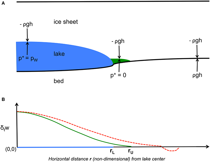
Figure 1. (A) Schematic of the obstacle problem (not to scale). The load above the lake (blue; r ≤ r_L), where the subglacial water pressure exceeds overburden [i.e., p⁺ > 0 in (16)], is the difference p_W − ρgh. Outside the lake (r > r_L), where overburden has not been reached (i.e., p⁺ = 0), any ice lifted above the bed (green) bears its own weight. (B) r_U is the largest radius for which the uplift rate ∂_tw (green line) is nonnegative everywhere. Attempting to set r > r_U as the radius of the uplift area results instead in an unphysical solution in which the ice is sinking into the bed (red dashed line).

We have so far set up the viscous obstacle problem for uplift of the ice-sheet area surrounding a subglacial lake at one given time. We first solve this problem over a broad range of parameters, before returning in the Discussion to consider the likely effects over time of flexural uplift on the (modeled) hydrological system.

2.3. Implementation

The flexure equations are solved by the finite element method, using the GetFEM++ library (Y. Renard and J. Pommier, http://getfem.org) via its MATLAB interface. GetFEM++ allows the use of higher order elements that can directly handle clamped boundary conditions; we use the third-order, continuously differentiable Hsieh-Clough-Tocher triangular element (Ciarlet, 1978). We use a mesh with over 9,000 nodes, generated by the DistMesh MATLAB package (Persson and Strang, 2004), which provides a highly uniform mesh over a disk while allowing us to require a node at the origin. We apply a simple bisection method to solve for the largest r such that ∂_tw ≥ 0 everywhere within the circle of radius r.

3. Experiments

3.1. The Viscous Obstacle Problem

We consider the obstacle problem (17) over a reasonable range of the nondimensional variables η, h, p, and r_L, with Γ given by the chosen scales for the problem. For simplicity, we assume spatially constant ice thickness h and viscosity η (i.e., D_nc = 0), and consider spatially variable h in section 3.3. The nondimensional results are easiest to evaluate if the scalings are taken from a solution of the dimensional problem. In this case, we use H = 1,000 m, R = 5,000 m, V = 10¹⁸ Pa s, and W_t = 0.10 m a⁻¹.

With variable bed topography, we expect real lakes (or at least lakes in subglacial hydrological models, e.g., Dow et al., 2016) to have maximum pressure at some point inside the lake, with pressure decreasing more gradually to overburden at the lake boundary. (For our purposes in this study, zero pressure above overburden defines the lake boundary.) Many different pressure distributions meeting these conditions are possible. For a smooth profile, we take the shape of the pressure above overburden to be a cubic function:

$\begin{array}{ll}{p}^{*}=1-\frac{3}{r_L^2}{\left(\sqrt{x^2+y^2}\right)}^2+\frac{2}{r_L^3}{\left(\sqrt{x^2+y^2}\right)}^3,x^2+y^2\le r_L^2& (20)\end{array}$

so that p* = 1 at the lake center and p* = 0 at and outside the lake boundary r_L, and its derivative is zero at both the center and the boundary. The full pressure above overburden is then p* multiplied by the maximum nondimensional value p_max at the lake center, so that $p^{+}-h=p^{*}·p_{max}$ over the lake.

We find that neither Γ nor η affects the solution for r_U, though the resulting solution for ∂_tw at radius r_U is directly proportional to Γ and inversely proportional to η. Furthermore, r_U scales with r_L; that is, the ratio of uplift radius to lake radius is independent of the size of the lake.

We are left to consider the effects of the nondimensional pressure p and thickness h on the solution of the obstacle problem. The range of ice thicknesses for which subglacial lakes have been observed is well known; here we will use 500–3,000 m. However, water pressure in subglacial lakes is not well constrained. In current subglacial hydrological models that are not yet coupled to ice flexure models, the modeled water pressure in lakes can become quite high as it is not eased by uplift. We therefore run the model across a very broad range of pressures above overburden, from 5 to 1,000 kPa. Figures 2, 3 show model results for low and high pressures, plotted separately for ease of viewing. Figure 4 presents the results in terms of ice thickness to emphasize the nonlinearity with respect to this variable.

FIGURE 2

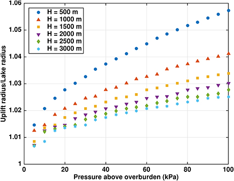
Figure 2. Ratio r_U/r_L of uplift radius to lake radius for lake pressures up to 1 bar above ice overburden pressure [using the cubic profile (20)] and typical ice thicknesses H.

FIGURE 3

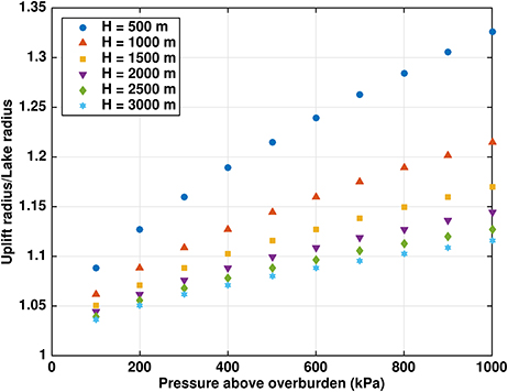
Figure 3. Ratio r_U/r_L of uplift radius to lake radius for lake pressures up to 10 bars above ice overburden pressure [using the cubic profile (20)] and typical ice thicknesses H.

FIGURE 4

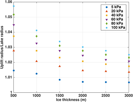
Figure 4. Ratio r_U/r_L of uplift radius to lake radius for selected lake pressures up to 1 bar above ice overburden pressure [using the cubic profile (20)], plotted against ice thickness to emphasize nonlinearity with respect to this variable.

Figures 2, 3 show that r_U/r_L for a given ice thickness is a weakly nonlinear function of the pressure above overburden, particularly for lower pressures. For example, the H = 1, 000 m results in Figure 2 can be linearly fitted with adjusted coefficient of determination ${\bar{R}}^2=0.969$ (not to be confused with the radius scale R), although the shape of the fit and the individual residuals are much better with a cubic (${\bar{R}}^2=0.998$) fit. In contrast, r_U/r_L for a given pressure above overburden (Figure 4) is a more strongly nonlinear function of ice thickness. For example, the 100 kPa pressure above overburden results can be linearly fitted with an ${\bar{R}}^2$ of only 0.814, but a cubic fit (consistent with the dependence of ice stiffness on thickness) produces a much better agreement (${\bar{R}}^2=0.998$).

3.2. The Viscous Obstacle Problem for Elliptical Lakes

Because subglacial lakes vary in shape, solving the obstacle problem for noncircular lakes is clearly important. We can make a start toward determining the effect of lake shape by considering elliptical lakes. For simplicity, we assume spatially constant ice thickness h and viscosity. If we repeat the derivation of (17) using scales of A for x and B for y (instead of R for both), we arrive at:

$\begin{array}{ll}\eta h^3\left[{\partial }_x^4+2{\left(\frac{a}{b}\right)}^2{\partial }_x^2{\partial }_y^2+{\left(\frac{a}{b}\right)}^4{\partial }_y^4\right]{\partial }_{t}w=a^4{\Gamma }_A(p^{+}-h),& (21)\end{array}$

where a_L is the lake's minor semiaxis length, Γ_A is (19) with A replacing R, and as before all lower case variables are nondimensional. The shape of the pressure above overburden is a version of (20) recast for an ellipse:

$\begin{array}{l}{p}^{*}=1-\frac{3}{a_L^2}{\left(\sqrt{x^2+{\left(\frac{a}{b}\right)}^2{y}^2}\right)}^2+\frac{2}{a_L^3}{\left(\sqrt{x^2+{\left(\frac{a}{b}\right)}^2{y}^2}\right)}^3,\\ x^2+{\left(\frac{a}{b}\right)}^2{y}^2\le a_L^2.& (22)\end{array}$

Similar to the circular case, we iterate to find the maximum a such that ∂_tw ≥ 0 everywhere within the ellipse with minor semiaxis length a and major semiaxis length b, calling the solution a_U. By setting up the obstacle problem to be solved for only one of the nondimensional semiaxis lengths, we have assumed that the uplift area will have the same shape as the lake, with the ratio of the semiaxis lengths fixed at a/b. This assumption, which seems reasonable for an initial study, allows the obstacle problem to be solved by a tractable one-parameter iteration.

Having already explored the effects of the other parameters in the a = b circular case, we focus on changing the shape of the lake by varying a/b. We note that a_U/a_L shows the same scale independence as r_U/r_L for (17), so we can consider only a/b without concern for the size of the lake. The results (Figure 5) show that lake shape does indeed matter. With the assumption that the uplift area has the same shape as the lake, a circular lake produces the largest relative uplift area, and any narrowing by reducing a/b results in progressively smaller relative uplift areas. However, the maximum uplift rate ∂_tw_max is nearly inversely proportional to a/b, slightly more than doubling for a/b = 0.5.

FIGURE 5

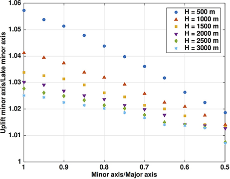
Figure 5. Ratio a_U/a_L of uplift minor axis to lake minor axis for ellipses of varying shape (using the cubic profile (22) with maximum overpressure 100 kPa). Note that results for equal major and minor axes match results for circular lakes (Figure 2), as expected.

3.3. Varying Ice Thickness

Due to the effects of topography and basal friction, it is reasonable to expect the ice above a lake to vary in thickness. For nonconstant ice thickness h, we solve (17) with the D_nc terms included. To vary the thickness, we choose a cubic function similar to our pressure distribution (20):

$\begin{array}{l}{h}^{*}=h_0+\frac{1}{r_L^2}(3-3h_0){\left(\sqrt{x^2+y^2}\right)}^2\\ +\frac{1}{r_L^3}(2h_0-2){\left(\sqrt{x^2+y^2}\right)}^3,x^2+y^2\le r_L^2& (23)\end{array}$

where h₀ is the relative thickness at the lake center, h* = 1 at the lake boundary, and the derivative is zero at both the center and the boundary. Ice thickness h above the lake is then h* scaled by the maximum (constant) value of thickness outside the lake.

As expected, r_U/r_L does increase for thinner ice and decrease for thicker ice over the lake (Figure 6). For example, r_U/r_L changes by ~ 0.006 (H = 500 m) and ~ 0.001 (H = 3, 000 m) for ± 10% thickness change at the center of the lake (using the cubic profile (20) with 100 kPa maximum overpressure). The maximum uplift rate increases approximately linearly with thinning, increasing for example by ~ 10.5% for 10% thinning of H = 1, 000 m and 100 kPa maximum overpressure. The effect of spatial variations in the ice thickness over the lake by up to ± 10% is very similar to that caused by ± 10% changes in the ice thickness in the “constant thickness” case (section 3.1), with differences in r_U/r_L on the order of 1 × 10⁻⁴. Given this result and the nonlinear dependence of r_U/r_L on ice thickness, moderate thinning or thickening over the lake can noticeably affect the size of the uplift area.

FIGURE 6

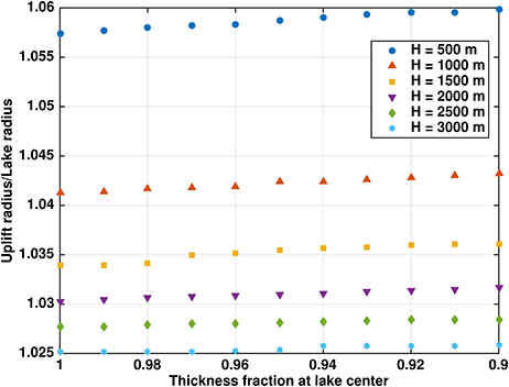
Figure 6. Ratio r_U/r_L of uplift radius to lake radius for spatially variable ice thickness above the lake [using the cubic profile (20) with maximum overpressure 100 kPa]. Thickness profiles are as given by (23).

3.4. Effects of Overpressure Distribution

As noted earlier, different plausible profiles for water pressure across a lake can be supposed. In order to better determine the effect of the overpressure distribution, we introduce several new functions to complement the cubic function (20) used in section 3.1:

$\begin{array}{ll}{p}^{*}=1-\frac{1}{r_L}\sqrt{x^2+y^2},(Linear)& (24)\end{array}$

$\begin{array}{ll}{p}^{*}=0.75\left[1-\frac{1}{r_L^2}{\left(\sqrt{x^2+y^2}\right)}^2\right],(Quadratic)& (25)\end{array}$

and

$\begin{array}{ll}{p}^{*}=0.6\left[1-\frac{1}{r_L^5}{\left(\sqrt{x^2+y^2}\right)}^5\right].(Quintic)& (26)\end{array}$

These functions are chosen to be one at the lake center and zero at and outside the boundary r_L, and scaled to have the same integrated overpressure as the cubic function (Figure 7). We repeat the (constant ice thickness) experiments shown in Figure 2 with the new pressure distributions. There is some dependence of r_U/r_L on the pressure distribution (Figure 8), with r_U/r_L varying by about 0.005 across the different profiles for H = 1, 000 m and 100 kPa maximum overpressure. The quintic profile, which has the highest overpressure near the lake boundary (Figure 7), results in the highest r_U/r_L, while the cubic profile, the most concentrated toward the lake center, results in the lowest r_U/r_L. Conversely, the maximum nondimensional uplift rate ∂_tw_max is greatest for the cubic profile and smallest for the quintic profile, although the differences are small ($\Delta {\partial }_t{w}_{max}<2.5\times 10^{-3}$ for H = 1, 000 and 100 kPa maximum overpressure, and an order of magnitude smaller for thicker ice).

FIGURE 7

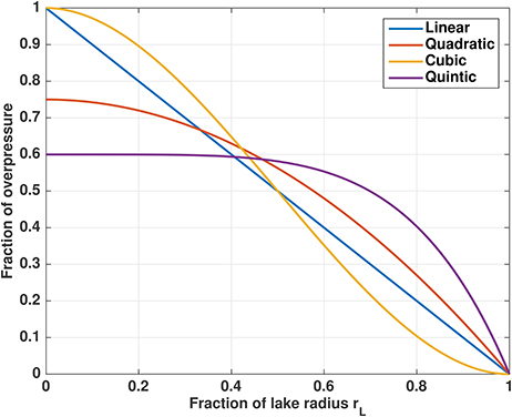
Figure 7. Functions $p^{*}(\sqrt{x^2+y^2})$ used to scale pressure above overburden in section 3.4. The cubic function is our standard distribution in all other sections.

FIGURE 8

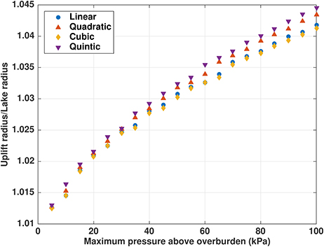
Figure 8. Ratio r_U/r_L of uplift radius to lake radius for maximum lake overpressure up to 1 bar, with 1,000 m ice thickness. Pressure distributions across the lake are as shown in Figure 7.

3.5. The Elastic Obstacle Problem

Had we instead taken the elastic limit (η → ∞) in (5)–(7) and repeated the derivation of the plate bending model, we would have arrived at an equation of the same form as (15), except solving for the uplift w instead of the uplift rate ∂_tw and with D = Eh³/9 instead of ηh³/6. Solving the analogous obstacle problem shows that the uplift w depends inversely on the elastic modulus E, and that the solution for r_U/r_L depends on h and p in exactly the same way as in the viscous case. It follows that the full viscoelastic obstacle problem needs to be solved for only one radius.

4. Discussion

We have seen that the solution to the ice flexure problem for subglacial lakes, which includes the relative area of uplift and the associated uplift (rate), depends on only a few parameters. The geometry of the lake and the overlying ice should be well known, and the material parameters (viscosity and/or Young's modulus) can be tuned to match observed lake growth and drainage. However, the water pressure in a subglacial lake is another vitally important variable whose range and spatial distribution are difficult to observe or constrain.

For the lower range of pressures used in this study (≲ 1 bar), the uplift area may be only a few percent larger than the lake area. Depending on the size of the lake, this may be less than the average mesh spacing of the hydrological model, and therefore require mesh refinement to resolve. Also, when r_U/r_L is relatively small (as will be the case early in the development of a lake) the uplift rate outside the lake is small relative to its maximum inside. For example, the cubic overpressure profile gives r_U/r_L = 1.04 when H = 1, 000 m and water pressure is 1 bar above overburden (Figure 2). Examining the shape of the uplift rate solution (Figure 9; cf. the fourth-order exact solution to the laccolith problem in Turcotte and Schubert, 2002), we see considerable flattening near r_U, so that the solution at the edge of the lake is <0.3% of the maximum value at the center. For typical uplift rates on the order of meters per year near the lake center (Gray et al., 2005; Fricker et al., 2010, 2014), the uplift rate between r_L and r_U will be on the scale of only millimeters per year. However, while the uplift rate in this area is small, solving the iterative obstacle problem for r_U > r_L instead of assuming that uplift occurs only over the lake (r_U = r_L) significantly affects the solution for ∂_tw. At each time step, the modeled uplift rate across the lake is higher when uplift outside the lake is considered (Figure 9).

FIGURE 9

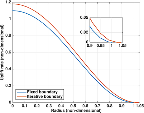
Figure 9. Nondimensional solutions of (17) for uplift rate, illustrating the decline in relative magnitude of the solution for ∂_tw toward the boundary and the difference between the results for a fixed boundary at the lake edge (r_U = r_L) vs. solving the obstacle problem for r_U > r_L. Note that at nondimensional radius 1 (the edge of the lake) ∂_tw for the iterative solution is < 0.3% of its maximum value at the lake center. Solutions are for H = 1, 000 m using the cubic profile (20) with maximum overpressure 100 kPa. Inset shows detail around the lake edge.

Returning to the entire hydrological system, we now explain the applicability of the flexure calculation to a future fully coupled ice sheet-hydrological model. The solution of (17) for ∂_tw provides the uplift rate over and surrounding a lake at a given time, which should affect water thickness throughout the domain in a way that tends toward reducing p_w in this area, relieving possibly nonphysical pressure buildups in hydrological models without ice sheet flexure. Hydrological models that allow the sheet thickness to evolve (e.g., Werder et al., 2013) contain an opening rate o due to ice sliding over obstacles and a closing rate c due to viscous creep, and the flexural uplift rate ∂_tw should behave similarly. We can add this rate to the water sheet continuity equation (e.g., Flowers, 2015) to obtain:

$\begin{array}{ll}\nabla ·\overrightarrow{q}+o-c+{\partial }_{t}w=m& (27)\end{array}$

where the discharge $\overrightarrow{q}$ is a function of the sheet thickness and the hydraulic gradient, and m is a source term. Given the low uplift rate between r_L and r_U, as discussed above, we expect changes in the water thickness and therefore the alteration of water pressure in this region to be negligible during the calculation of ∂_tw at one time step. However, we expect that ∂_tw and p_w will be interdependent over multiple adaptive time steps, allowing the area of the lake to gradually increase. Further exploration of these ideas will have to await development of a fully coupled model across a catchment.

In order to couple an ice flexure model with a hydrological model, several challenges need to be overcome. First, the hydrological model must be able to form and identify lakes. Second, areas containing lakes must be (re)meshed in a manner that enables solution of the obstacle problem. While we have worked here with relatively simple shapes, we suggest a similar single-parameter scaling for more realistic shapes as a reasonable and computationally tractable initial approach. Third, the uplift rate calculated by the flexure model must be incorporated into the hydrological model equations. In the case of rapid and significant pressure changes (e.g., Greenland supraglacial lake drainage to the bed), the uplift calculation may require simultaneous and/or iterative solution of both sets of equations, with uplift (rate) immediately impacting the pressure calculated by the hydrological model and vice versa. However, in the viscous-dominated Antarctic case with longer timescales it is likely that the uplift will just contribute another rate (in addition to cavity opening and closing rates) in the equation for time evolution of water sheet thickness (e.g., Werder et al., 2013).

5. Conclusion

We have developed a viscous model of plate bending suitable for ice-sheet flexure caused by basal water pressure in excess of overburden. Applying this model to solve the obstacle problem associated with possible uplift outside a subglacial lake, we find that ice thickness and subglacial water pressure determine the relative size of the uplift area, while the viscous material properties of ice scale the magnitude of the uplift rate within this area. Although we use only circular and elliptical lakes in this study, we find that the ratio of uplift area to lake area scales with lake size, and that lake shape has a significant effect. The distribution of overpressure across a lake also affects the solution of the obstacle problem, with greater weighting toward the boundary producing higher ratios of uplift area to lake area, but greater weighting toward the lake center producing higher maximum uplift rates. Ice thickness profiles that are moderately thinner over the lake also result in higher ratios of uplift area to lake area, although the effect is relatively small.

Because water pressure in subglacial lakes is not well constrained (due to lack of observations and limited incorporation of ice flexure effects in current hydrological models), the importance of solving the obstacle problem for coupled models of subglacial lakes remains unknown at this time. Where direct observations of subglacial water pressure are not available, we suggest that coupled modeling of low-pressure scenarios where uplift outside the lake can (temporarily) be neglected could provide preliminary estimates of the relationship between water pressure and uplift. We do, however, expect that ice flexure will affect lake filling and draining (and thus ice flow), and therefore the development of a realistic coupled model incorporating the insights gained in this study is a necessary and important goal.

Author Contributions

All authors contributed to the theory underlying this work. RW coded the model and ran the experiments. All authors contributed to analysis of the results and participated in writing this manuscript.

Funding

RW was supported by the NSF under grant PLR-1443284 and by NASA under grant NNX12AD03A. CD was supported by a NASA Postdoctoral Program fellowship at Goddard Space Flight Center. Additional funding was provided to SN by NASA through its Cryospheric Sciences and Modeling Analysis and Prediction programs.

Conflict of Interest Statement

The authors declare that the research was conducted in the absence of any commercial or financial relationships that could be construed as a potential conflict of interest.

Acknowledgments

We thank the editor and reviewers for constructive comments that led to a greatly improved final manuscript.

References

Bartholomaus, T. C., Anderson, R. S., and Anderson, S. P. (2008), Response of glacier basal motion to transient water storage. Nat. Geosci. 1, 33–37. doi: 10.1038/ngeo.2007.52

CrossRef Full Text | Google Scholar

Bartholomew, I., Nienow, P., Sole, A., Mair, D., Cowton, T., and King, M. A. (2012). Short-term variability in Greenland Ice Sheet motion forced by time-varying meltwater drainage: implications for the relationship between subglacial drainage system behavior and ice velocity. J. Geophys. Res. 117:F03002. doi: 10.1029/2011JF002220

CrossRef Full Text | Google Scholar

Boresi, A. P., and Schmidt, R. J. (2003). Advanced Mechanics of Materials. New York, NY: John Wiley & Sons.

Google Scholar

Carter, S. P., Fricker, H. A., Blankenship, D. D., Johnson, J. V., Lipscomb, W. H., Price, S. F., et al. (2011). Modeling 5 years of subglacial lake activity in the MacAyeal Ice Stream (Antarctica) catchment through assimilation of ICESat laser altimetry. J. Glaciol. 57, 1098–1112. doi: 10.3189/002214311798843421

CrossRef Full Text | Google Scholar

Carter, S. P., and Fricker, H. A. (2012). The supply of subglacial meltwater to the grounding line of the Siple Coast, West Antarctica. Ann. Glaciol. 53, 267–280. doi: 10.3189/2012AoG60A119

CrossRef Full Text | Google Scholar

Ciarlet, P. G. (1978). The Finite Element Method for Elliptic Problems. Amsterdam: North-Holland.

Google Scholar

Dow, C. F., Kulessa, B., Rutt, I. C., Tsai, V. C., Pimentel, S., Doyle, S. H., et al. (2015). Modeling of subglacial hydrological development following rapid supraglacial lake drainage. J. Geophys. Res. Earth Surf. 120, 1127–1147. doi: 10.1002/2014JF003333

PubMed Abstract | CrossRef Full Text | Google Scholar

Dow, C.F., Werder, M. A., Nowicki, S., and Walker, R. T. (2016). Modeling Antarctic subglacial lake filling and drainage cycles. Cryosphere 10, 1381–1393. doi: 10.5194/tc-10-1381-2016

CrossRef Full Text | Google Scholar

de Fleurian, B., Gagliardini, O., Zwinger, T., Durand, G., Meur, E. L., Mair, D., et al. (2014). A double continuum hydrological model for glacier applications. Cryosphere 8, 137–153. doi: 10.5194/tc-8-137-2014

CrossRef Full Text | Google Scholar

Einarsson, B., Jóhannesson, T., Thorsteinsson, T., Gaidos, E., and Zwinger, T. (2017). Subglacial flood path development during a rapidly rising jökulhlaup from the western Skaftá cauldron, Vatnajökill, Iceland. J. Glaciol. 63, 670–682. doi: 10.1017/jog.2017.33

CrossRef Full Text | Google Scholar

Evatt, G. W., Fowler, A. C., Clark, C. D., and Hulton, N. R. J. (2006). Subglacial floods beneath ice sheets. Phil. Trans. R. Soc. A 364, 1769–194. doi: 10.1098/rsta.2006.1798

PubMed Abstract | CrossRef Full Text | Google Scholar

Evatt, G. W., and Fowler, A. C. (2007) Cauldron subsidence subglacial floods. Ann. Glaciol. 45, 163–168. doi: 10.3189/172756407782282561

CrossRef Full Text | Google Scholar

Evans, L. C. (1998). Partial Differential Equations, 2nd Edn. Providence, RI: American Mathematical Society.

Google Scholar

Flowers, G. E. (2015). Modelling water flow under glaciers and ice sheets. Proc. R. Soc. A 471:20140907. doi: 10.1098/rspa.2014.0907

PubMed Abstract | CrossRef Full Text | Google Scholar

Fricker, H. A., Scambos, T., Bindschadler, R., and Padman, L. (2007). An active subglacial water system in West Antarctica mapped from space. Science 315, 1544–1548. doi: 10.1126/science.1136897

PubMed Abstract | CrossRef Full Text | Google Scholar

Fricker, H. A., Scambos, T., Carter, S. P., Davis, C., Haran, T., and Joughin, I. (2010). Synthesizing multiple remote-sensing techniques for subglacial hydrologic mapping: application to a lake system beneath MacAyeal Ice Stream, West Antarctica. J. Glaciol. 56, 187–199. doi: 10.3189/002214310791968557

CrossRef Full Text | Google Scholar

Fricker, H. A., Carter, S. P., Bell, R. E., and Scambos, T. (2014). Active lakes of Recovery Ice Stream, East Antarctica: a bedrock-controlled subglacial hydrological system. J. Glaciol. 60, 1015–1030. doi: 10.3189/2014JoG14J063

CrossRef Full Text | Google Scholar

Gray, L., Joughin, I., Tulaczyk, S., Spikes, V. B., Bindschadler, R., and Jezek, K. (2005). Evidence for subglacial water transport in the West Antarctic Ice Sheet through three-dimensional satellite radar interferometry. Geophys. Res. Lett. 32:L03501. doi: 10.1029/2004GL021387

CrossRef Full Text | Google Scholar

Hewitt, I. J. (2013). Seasonal changes in ice sheet motion due to melt water lubrication. Earth Planet. Sci. Lett. 371–372, 16–25. doi: 10.1016/j.epsl.2013.04.022

CrossRef Full Text | Google Scholar

Iken, A., and Bindschadler, R. A. (1986). Combined measurements of subglacial water pressure and surface velocity of Findelengletscher, Switzerland: conclusions about drainage system and sliding mechanism. J. Glaciol. 32, 101–119. doi: 10.1017/S0022143000006936

CrossRef Full Text | Google Scholar

Kamb, B. (1987). Glacier surge mechanism based on linked cavity configuration of the basal water conduit system. J. Geophys. Res. 92, 9083–9099. doi: 10.1029/JB092iB09p09083

CrossRef Full Text | Google Scholar

MacAyeal, D. R., Sergienko, O. V., and Banwell, A. F. (2015). A model of viscoelastic ice-shelf flexure. J. Glaciol. 61, 635–645. doi: 10.3189/2015JoG14J169

CrossRef Full Text | Google Scholar

Pattyn, F. (2008). Investigating the stability of subglacial lakes with a full stokes ice-sheet model. J. Glaciol. 54, 353–361. doi: 10.3189/002214308784886171

CrossRef Full Text | Google Scholar

Persson, P.-O., and Strang, G. (2004). A simple mesh generator in MATLAB. SIAM Rev. 46, 329–345. doi: 10.1137/S0036144503429121

CrossRef Full Text | Google Scholar

Siegfried, M. R., Fricker, H. A., Roberts, M., Scambos, T. A., and Tulaczyk, S. (2014). A decade of West Antarctic subglacial lake interactions from combined ICESat and CryoSat-2 altimetry. Geophys. Res. Lett. 41, 891–898. doi: 10.1002/2013GL058616

CrossRef Full Text | Google Scholar

Tsai, V. C., and Rice, J. R. (2010). A model for turbulent hydraulic fracture and application to crack propagation at glacier beds. J. Geophys. Res. Earth Surf. 115:F03007. doi: 10.1029/2009JF001474

CrossRef Full Text | Google Scholar

Turcotte, D. L., and Schubert, G. (2002). Geodynamics, 2nd Edn. New York, NY: Cambridge University Press.

Werder, M. A., Hewitt, I. J., Schoof, C. G., and Flowers, G. E. (2013). Modeling channelized and distributed subglacial drainage in two dimensions. J. Geophys. Res. Earth Surf. 118, 2140–2158. doi: 10.1002/jgrf.20146

CrossRef Full Text | Google Scholar