Petrological Geodynamics of Mantle Melting II. AlphaMELTS + Multiphase Flow: Dynamic Fractional Melting

Introduction

Melting in the Earth's and planetary interiors is usually approached either from a physical perspective based on geophysical tools (e.g., seismology) and numerical studies based on dynamic two-phase flow models, or from a petrological perspective that focuses mainly on the chemical evolution of the melt products and minerals. In the first installment (Tirone and Sessing, 2017), hereafter called MF1, a petrological and dynamic numerical model has been introduced with the aim to develop a dynamic and petrological representation of the melting process in the Earth's mantle. The general motivation was that the classical petrological descriptions of melting, namely batch melting and fractional melting are physically flawed. Batch melting implies that melt products stay always in contact with the source, an implausible scenario for mantle melting, except for the cases in which only tiny amount of melt pockets are the end-product. Fractional melting would imply that no melt would exist in the mantle since all melt is immediately extracted. Both are also static atemporal models, the mantle doesn't move and the melt either doesn't move or disappears instantaneously. Time is also irrelevant. To remove these unreal physical limitations the dynamic model, exemplified by a 1-D mantle column, has been formulated considering the presence of two or three dynamic phases (solid, melt or solid, melt and water). The petrological and chemical description is provided by the program AlphaMELTS (Smith and Asimow, 2005) (pMELTS version) which is based on the thermodynamic model developed by Ghiorso over several years (Ghiorso, 1985; Ghiorso and Sacks, 1995; Ghiorso et al., 2002). The ability of the earlier version of MELTS to reproduce observable and experimental data was evaluated in a series of studies (Hirschmann et al., 1998, 1999a,b; Asimow et al., 2001). A thermodynamic model is not an absolute requirement. A petrological tool based on melting parameterization has been developed recently (Brown and Lesher, 2016), and in principle it could be used in combination with some dynamic model as well. Numerous studies investigated the dynamic evolution of melt and solid mantle using a two-phase flow model (McKenzie, 1984; Scott and Stevenson, 1984, 1986; Spiegelman, 1993; Richardson, 1998; Ghods and Arkani-Hamed, 2000; Schmeling, 2000; Bercovici et al., 2001; Bercovici and Ricard, 2003; Spiegelman et al., 2007; Hewitt and Fowler, 2008; Katz, 2008; Hewitt, 2010; Rudge et al., 2011; Oliveira et al., 2018). The most recent one (Oliveira et al., 2018) incorporates a complex rheology and a realistic thermodynamic equilibrium model.

The numerical solution and the details of the coupled petrological and geodynamic 1-D model applied here have been presented in the previous study, MF1. The concept of dynamic equilibrium melting (DEM) was also introduced in MF1. Essentially it assumes chemical, thermal and mechanical equilibrium between solid and melt over a certain spatial and temporal interval. Even though some form of hybrid kinetic-thermodynamic petrological modeling can be conceived (Tirone et al., 2016), and a dynamic melting formulation based on simplified kinetic principles has been considered already (Rudge et al., 2011), this series of contributions focuses exclusively on the domain defined by thermodynamic equilibrium principles. The reason is that as soon as the petrological batch and fractional melting models are put in a real physical context, the spatial and temporal extension of chemical equilibration can still be interpreted rather freely. Hence it seems reasonable to devote first some effort trying to understand the consequences of different possible equilibrium scenarios.

One of these scenarios may be described by a model in which the melt cumulative products are chemically isolated from the local residual solid. It is a common practice in petrology to consider this fractional melting process to explain and model certain geochemical and petrological evidences (e.g., Langmuir et al., 1992; Herzberg and Asimow, 2008; Hole, 2015; Rey, 2015; Carr and Gazel, 2017). However the concept of fractional melting is usually applied without any assumption on the temporal and spatial constraints. Therefore a logical step forward would be to investigate the outcome of a fractional melting process that develops dynamically inside the mantle and evolves over time under certain equilibrium assumptions. This would be also the simplest description of melting departing from the assumption of complete local equilibrium between solid and melt. Such model called dynamic fractional melting (DFM) is the main subject of this study. Asimow (2002) developed the conceptual original idea and first implementation of dynamic fractional melting. The work presented here could be considered an extension of this earlier model in the sense that it removes certain restrictions of the previous implementation. For instance in the current formulation the properties are time dependent, the flow pressure is computed explicitly (relative to a fixed point), the melt velocity is not assumed to be much greater than the solid velocity and no restriction is imposed on the density of melt. This study also presents the complete set of compositional/petrological results and applies the latest thermodynamic melt model for mantle melting, pMELTS (Ghiorso et al., 2002), that at the time of the original development was not available.

The main features and the recipe for a practical implementation of a petrological dynamic melting model have been presented in MF1, therefore mainly new aspects of the DFM model will be discussed in the following sections. The DFM model is presented in the next section “Description of the Dynamic Fractional Melting Model”. It is followed in section “Changes in the Thermodynamic Computation” by a discussion of the modifications that need to be implemented to the thermodynamic computation. The section “Changes to the Mass Conservation Equations” begins to outline the changes to the transport model, and includes a brief summary of the transport equations.

The results of the DFM model are first compared with the equilibrium dynamic melting model DEM presented in MF1. Only the effect of certain parameters are then investigated, in particular the temperature at the base of the mantle column, the upwelling velocity of the solid at the boundary and the assumption of passive and active flow approximately represented by a fixed velocity either at the top or bottom boundary. All the results are presented in the section “Results of the Dynamic Fractional Melting Model”.

Description of the Dynamic Fractional Melting Model

The general idea of the DFM model is illustrated in Figure 1. At every grid point the representative space is occupied by two sub-systems, sub-sys 1 (ss1) and sub-sys 2 (ss2), each of the two developing separate chemical equilibration pathways. The first sub-system is only filled by the solid mantle (and a free water phase, if present in the system), while the second sub-system consists of melt and a different solid that may form by partial crystallization of the local melt. When the thermodynamic computation applied to the solid in ss1 predicts that partial melting will occur, the melt is transferred to the second sub-system associated to the same depth location and it will not interact chemically any further with the residual solid. In this way the first sub-system is always free of melt. The second sub-system consists essentially of a cumulate melt, however chemical thermodynamics is applied to this sub-system as well to determine whether partial crystallization may take place or whether a free water phase would form at equilibrium. If new solid crystallizes, it remains in ss2 while any amount of free water is transferred in ss1. Both the aggregate melt and the fractionated solid do not interact chemically with the solid in ss1. However from a dynamic point of view, the two solids are assimilated to a single transport phase. Melt is treated as a separated dynamic phase, while the free water phase (if present) is considered the third dynamic phase.

FIGURE 1

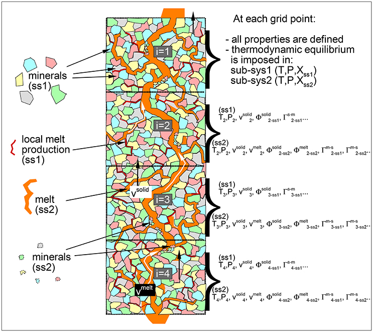
Figure 1. Schematic view of the mantle melting column. In the dynamic fractional melting (DFM) model at each grid point local equilibrium is assumed separately for the residual solid and for melt in two sub-systems. Dynamic and thermodynamic properties represent the average spatial values within each sub-system. Melt formed in the first sub-system (sub-sys1) is transferred in the second sub-system (sub-sys2). Melt in sub-sys2 is allowed to crystallize but the new solid remains in sub-sys2. Distribution of melt and minerals in the figure not in scale. The illustration describes only one possible visual interpretation of the model regarding the melt and solids distribution inside the representative spatial grid points. Details about the numerical discretization and numerical solution can be found in MF1.

The following sections explain how this process is modeled. The discussion in particular highlights the changes that have been applied to the previous formulation introduced in MF1.

Changes in the Thermodynamic Computation

The main difference in the thermodynamic approach between the DFM and the DEM model is that chemical equilibrium is maintained in two sub-systems separately, that is two separate thermodynamic computations are performed at every spatial grid point. The temperature and the pressure are assumed to be the same in the two sub-systems but the bulk composition is different. As in the previous study, the pressure applied in the thermodynamic computations is the lithostatic pressure and it is assumed to be the same in ss1 and ss2. The energy transport equation is solved for the temperature of the whole system (ss1+ss2) and does not include the viscous dissipation effect (small contribution, Asimow and Stolper, 1999; Tirone, 2016) and the latent heat of melting/crystallization. The latter has been neglected mainly because the numerical implementation presents challenges that cannot be easily addressed yet (Tirone et al., 2012).

The bulk abundance in wt % of a certain component c (oxide) for example in sub-system 1 at grid point i and time t, is computed using the following relation:

$\begin{array}{ll}bulkcomponent{c}_{ss1}=100({\Theta }_{i,t}^{{sc}_{ss1}}+{\Phi }_{i,t}^w)/({\Phi }_{i,t}^{s_{ss1}}+{\Phi }_{i,t}^w)& (1)\end{array}$

where the superscripts s, m, w indicate solid, melt and free water. ${\theta }_{i,t}^{{sc}_{ss1}}$ is the wt % of the component c defining the bulk composition of the solid in ss1, ${\Phi }_{i,t}^{s_{ss1}}$ is simply the product $({\rho }_{i,t}^{s_{ss1}}{\varphi }_{i,t}^{s_{ss1}})$ where ${\rho }_{i,t}^{s_{ss1}}$ is the mass density of the solid and ${\varphi }_{i,t}^{s_{ss1}}$ is the fraction of the control volume occupied by the solid. And last ${\Theta }_{i,t}^{{sc}_{ss1}}$ is the short notation for the product $({\rho }_{i,t}^{s_{ss1}}{\varphi }_{i,t}^{s_{ss1}}{\theta }_{i,t}^{{sc}_{ss1}})$. Since the free water phase (if present) is made only of H₂O, it follows that for example if c stands for MgO, then in the numerator of Equation (1), ${\Phi }_{i,t}^w$ should be set to zero.

In sub-system 2 a similar expression can be applied, bulk component $c_{ss2}=100 ({\Theta }_{i,t}^{{sc}_{ss2}}+{\Theta }_{i,t}^{mc})/({\Phi }_{i,t}^{s_{ss2}}+{\Phi }_{i,t}^m)$. It can be noted that the superscripts ss1 and ss2 are used only for the solid components, while melt is only located in sub-system 2 and water (if present) only in sub-system 1. The data extracted from the thermodynamic computation are the same that were discussed for the DEM model in the previous study. However in this case they are specific to a particular sub-system: total mass and wt % of oxides of the solid, thermal expansion of the whole sub-system, mass, volume, oxide bulk composition and heat capacity at constant pressure of the mineral components and similar quantities for melt and water. Heat capacity and density are then computed for the total solid, melt and water in each sub-system following a procedure similar to the one described in MF1.

Another significant difference with the previous model is that the computation of the volume fraction of an assemblage (solid in ss1 and ss2, melt in ss2, and water in ss1) with respect to the total volume of the two sub-systems does not simply require the volume of each assemblage, because the thermodynamic computations are applied to sub-systems occupying different portions of the total space associated to a particular grid point. The volume fraction of the solid in ss1 can be retrieved from the following expression:

$\begin{array}{ll}{\varphi }^{s_{ss1}}=\frac{({\Phi }^{s_{ss1}}+{\Phi }^w)\times volume{(s)}^{ss1}}{({\Phi }^{s_{ss1}}+{\Phi }^w)\times volume{(s+m+w)}^{ss1}+({\Phi }^{s_{ss2}}+{\Phi }^m)\times volume{(s+m+w)}^{ss2}}& (2)\end{array}$

where the various Φ are taken from the transport model and the volumes are computed from the thermodynamic model. Note that the volumes include solid melt, and water in both sub-systems before they are rearranged (e.g., newly formed melt transferred in ss2). Similar relations can be used to determine the volume fraction of solid in ss2, melt in ss2 and water in ss1, given that the sum must be equal to 1, ${\varphi }^{s_{ss1}}+{\varphi }^{s_{ss2}}+{\varphi }^m+{\varphi }^w=1$. The mass transfer is then computed for each sub-system following the procedure discussed in MF1. For example knowing the density and volume fraction of the solid in ss1 from the thermodynamic model, the mass transfer is:

$\begin{array}{ll}\Delta {\Phi }^{s_{ss1}}={(densityofsolid\times volumefractionofsolid)}^{ss1}-{\Phi }^{s_{ss1}}& (3)\end{array}$

and similarly for the solid in ss2. Since no melt is present in ss1 before the thermodynamic computation is applied (all previous melt was already transferred to ss2), the mass transfer for melt in ss1 is defined as $\Delta {\Phi }^{m_{ss1}}=$[(density of melt × volume fraction of melt)^ss1], which is always ≥ 0. Melt in ss2 can also crystallize, therefore the melt transfer in ss2 is $\Delta {\Phi }^{m_{ss2}}=$[(density of melt × volume fraction of melt)^ss2−Φ^m]. For water in ss1 $\Delta {\Phi }^{m_{ss1}}=$[(density of water × volume fraction of water)^ss1 - Φ^m] and when water is formed in ss2, $\Delta {\Phi }^{m_{ss2}}=$[(density of water × volume fraction of water)^ss2] since it was not present before the thermodynamic computation (all water was transferred already in ss1). The chemical mass transfer quantities follow the same principles, for example for the transfer of the chemical component c related to the solid in sub-system 1:

$\begin{array}{l}\Delta {\Theta }^{s{c}_{ss1}}=(density\times volumefraction-\\ \times bulkcompositionofoxidecinthesolid{)}^{ss1}-{\Theta }^{s{c}_{ss1}}& (4)\end{array}$

Summary of the Transport Equations

Before describing the changes in the dynamic model, the transport equations presented in MF1 are briefly summarized here. The conservation of mass for the total solid, melt and water separately is given by similar expressions assuming this general form:

$\begin{array}{ll}\frac{\partial ({\rho }^a{\varphi }^a)}{\partial t}+\frac{\partial (v^a{\rho }^a{\varphi }^a)}{\partial z}={\Gamma }^a& (5)\end{array}$

where v^a is the vertical velocity of the assemblage a and the mass transfer term Γ^a is not explicitly considered in the numerical solution model but instead it is incorporated in the mass at the previous time step. The equation of motion for the solid assemblage (ss1+ss2) is expressed as follow:

$\begin{array}{ll}-{\varphi }^s\frac{\partial P}{\partial z}+{\varphi }^s{\rho }^{s}g-M^{s-m}-M^{s-w}+S=0& (6)\end{array}$

where S encloses the description of the viscous forces which depend on the velocity of the solid. The M terms describe the dynamic coupling of motion of the assemblages, in general they are proportional to the difference of the velocities of two assemblages (e.g., s − m ⇒ solid − melt). The equation of motion for melt is given by the following expression:

$\begin{array}{ll}-{\varphi }^m\frac{\partial P}{\partial z}+{\varphi }^m{\rho }^{m}g+M^{s-m}=0& (7)\end{array}$

after replacing M^s−m with an expression that depends on the permeability, melt volume fraction and velocity difference, this equation is solved explicitly for the melt velocity v^m. For practical reasons the equation of motion for the solid assemblage (Equation 6) is not used in the numerical solution but a sum of the equations of motion for the three assemblages is applied instead:

$\begin{array}{ll}-\frac{\partial P}{\partial z}+{\varphi }^s{\rho }^{s}g+{\varphi }^m{\rho }^{m}g+{\varphi }^w{\rho }^{w}g+S=0& (8)\end{array}$

The three mass conservation equations (similar to Equation 5), the equation of motion for melt and water (Equation 7 for melt and a similar one for water), the total equation of motion (Equation 8) and the volume fraction constraint (ϕ^s+ϕ^m+ϕ^w = 1) are solved simultaneously by iteration following the procedure detailed in MF1 to retrieve the pressure (or pressure gradient), the volume fractions ϕ^s, ϕ^m, ϕ^w, and the respective velocities v^s, v^m, v^w. For every chemical components c in the solid and melt the transport equation is expressed in this form:

$\begin{array}{l}\frac{\partial ({\rho }^s{\varphi }^s{\theta }^{sc})}{\partial t}+\frac{\partial (v^s{\rho }^s{\varphi }^s{\theta }^{sc})}{\partial z}={\Gamma }^{sc-mc} ;\\ \frac{\partial ({\rho }^m{\varphi }^m{\theta }^{mc})}{\partial t}+\frac{\partial (v^m{\rho }^m{\varphi }^m{\theta }^{mc})}{\partial z}={\Gamma }^{mc-sc}& (9)\end{array}$

where the chemical mass transfer term (e.g., Γ^sc−mc) is absorbed in the chemical mass component at the previous time step in the same way that Γ^a was implicitly manipulated in the mass conservation equations. The temperature is described by the following relation:

$\begin{array}{l}\frac{\partial T}{\partial t}{\displaystyle \sum ^a}{C}_{p^a}{\rho }^a{\varphi }^a+\frac{\partial T}{\partial z}{\displaystyle \sum ^a}{v}^a{C}_{p^a}{\rho }^a{\varphi }^a=\frac{{\partial }^{2}T}{\partial z^2}{K}^{sys}+T\frac{\partial P}{\partial t}{\alpha }^{sys}\\ +T\frac{\partial P}{\partial z}{v}^{sys}{\alpha }^{sys}& (10)\end{array}$

where $C_{p^a}$ is the heat capacity at constant pressure of the assemblage a and K^sys and α^sys are the thermal conductivity and thermal expansion of the whole system and $v^{sys}\approx \sum _a{v}^a{\varphi }^a$. The last two terms in the above equation describe the reversible adiabatic effect due to compression or expansion. The effect of viscous dissipation has been ignored because it has a minor effect on the thermal profile over the considered depth interval (less than hundred kilometers). The heat change induced by chemical transformations (mainly melting) has been also excluded from the thermal model even though its overall contribution can be on the order of tens of degrees.

Changes to the Mass Conservation Equations

These transport equations are applied to the DFM model as well but some changes are necessary to account for the different interpretation of the DEM and DFM models. For instance considering the melt phase, it is not allowed to remain in the first sub-system and melt in the second sub-system can also crystallize. As in the DEM model, the melt transfer is added to the related term from the previous time step ${\Phi }_{i,(t-1)}^m$, however in this case it should include two quantities, one to describe the transfer from ss1 to ss2 ($\Delta {\Phi }^{m_{ss1}}$) and one for the change due to crystallization in ss2 ($\Delta {\Phi }^{m_{ss2}}$):

$\begin{array}{ll}{\Phi }_{i,(t-1)}^m={\Phi }_{i,(t-1)}^m+\frac{(\Delta {\Phi }^{m_{ss1}}+\Delta {\Phi }^{m_{ss2}})}{nthermo}& (11)\end{array}$

where nthermo is the number of time steps between two thermodynamic calculations. The definition of the two ΔΦ^m terms have been given in the previous section. The same numerical solution of the mass conservation equations for melt and water (Equation 5) outlined in MF1 is applied here. In the transport model the volume fraction of solid was retrieved from ϕ^s + ϕ^m + ϕ^w = 1. In the DFM model a second solid could be present in sub-system 2, therefore ϕ^s represents the sum of the solid volume fraction in ss1 and ss2, ${\varphi }^s={\varphi }^{s_{ss1}}+{\varphi }^{s_{ss2}}$. To find the volume fraction of the solid in each of the two sub-systems (${\varphi }^{s_{ss1}}$ and ${\varphi }^{s_{ss2}}$) after computing the total ϕ^s from the overall solution of the transport model, an additional step is needed. The ratio:

$\begin{array}{ll}R=\frac{{\Phi }_{i,(t-1)}^{s_{ss1}}}{{\Phi }_{i,(t-1)}^{s_{ss2}}}& (12)\end{array}$

is defined at the previous time step and includes the mass transfer terms. The assumption is that R remains unchanged at the current time. Recalling the definition of Φ = ρϕ, then for the solid in ss1, ${\Phi }_{i,t}^{s_{ss1}}={\rho }_{i,t}^{s_{ss1}}{\varphi }_{i,t}^{s_{ss1}}$ and replacing ${\Phi }_{i,t}^{s_{ss1}}$ with the ratio expression, $R {\Phi }_{i,t}^{s_{ss2}}={\rho }_{i,t}^{s_{ss1}}{\varphi }_{i,t}^{s_{ss1}}$, the volume fraction ${\varphi }_{i,t}^{s_{ss1}}$ can be found using:

$\begin{array}{ll}{\varphi }_{i,t}^{s_{ss1}}=\frac{R{\varphi }_{i,t}^{s_{ss2}}{\rho }_{i,t}^{s_{ss2}}}{{\rho }_{i,t}^{s_{ss1}}}& (13)\end{array}$

By replacing ${\varphi }_{i,t}^{s_{ss1}}$ with ${\varphi }^s-{\varphi }^{s_{ss2}}$ in the above equation, the volume fraction in ss2 can be expressed as:

$\begin{array}{ll}{\varphi }_{i,t}^{s_{ss2}}=\frac{{\varphi }_{i,t}^s}{\left(R\frac{{\rho }_{i,t}^{s_{ss2}}}{{\rho }_{i,t}^{s_{ss1}}}+1\right)}& (14)\end{array}$

With the above equation the volume fraction ${\varphi }_{i,t}^{s_{ss2}}$ can be computed knowing ${\varphi }_{i,t}^s$ from the transport model and the volume fraction constraint ($1-{\varphi }_{i,t}^m-{\varphi }_{i,t}^w$), and the densities ${\rho }_{i,t}^{s_{ss2}}$, ${\rho }_{i,t}^{s_{ss1}}$ from the thermodynamic model. Finally ${\varphi }_{i,t}^{s_{ss1}}$, ${\Phi }_{i,t}^{s_{ss1}}$ and ${\Phi }_{i,t}^{s_{ss2}}$ are then easily retrieved.

Changes to the SIMPLER and SIMPLECR Algorithm

The modifications to the SIMPLER or SIMPLECR algorithm are minimal because the velocity of the solids in the two sub-systems is assumed to be the same. Without the presence of free water the equation of motion for the whole system (Equation 8) and the mass conservation for the total solid (Equation 5) are still solved in four steps and the solution is iterated along with the equation of motion for melt (Equation 7) and mass conservation for melt (Equation 5) to find ${\Phi }_i^s$, ${\Phi }_i^m$, $v_i^s$, $v_i^m$ and P_i (or dP/dz_i. The only difference with the DEM model is the new definition of the total solid that is the sum of the solids in the two sub-systems ${\Phi }_{i,(t-1)}^s={\Phi }_{i,(t-1)}^{s_{ss1}}+{\Phi }_{i,(t-1)}^{s_{ss2}}$, and similar relations for ${\Phi }_{i,t}^s$ and ${\varphi }_{i,t}^s$.

Changes to the Temperature Equation

The computation of the temperature using Equation (10) follows closely the procedure already discussed in the previous study. The product $C_p^s{\Phi }^s$ is made of the sum of two terms, $C_{p_{i,t}}^s{\Phi }_{i,t}^s=C_{p_{i,t}}^{s_{ss1}}{\Phi }_{i,t}^{s_{ss1}}+C_{p_{i,t}}^{s_{ss2}}{\Phi }_{i,t}^{s_{ss2}}$. The thermal expansion of the whole system is the weighted average of the thermal expansion in the two sub-systems:

$\begin{array}{l}{\alpha }_{i,t}^{ss1}\frac{({\Phi }_{i,t}^{s_{ss1}}+{\Phi }_{i,t}^w)}{({\Phi }_{i,t}^{s_{ss1}}+{\Phi }_{i,t}^w+{\Phi }_{i,t}^{s_{ss2}}+{\Phi }_{i,t}^m)}\\ +{\alpha }_{i,t}^{ss2}\frac{({\Phi }_{i,t}^{s_{ss2}}+{\Phi }_{i,t}^m)}{({\Phi }_{i,t}^{s_{ss1}}+{\Phi }_{i,t}^w+{\Phi }_{i,t}^{s_{ss2}}+{\Phi }_{i,t}^m)}& (15)\end{array}$

Thermal conductivity of the two solids is assumed to be the same.

Changes to the Transport Equation for the Composition

The same chemical transport equation used in MF1 (Equation 9) is also applied to the DFM model to determine the composition of the melt and the total solid. Following the procedure for the solution of the mass transport model, the chemical transfer for the total solid is added to the value of ${\Theta }_{i,(t-1)}^{sc}$ at the previous time step and includes two terms, ${\Theta }_{i,(t-1)}^{sc}={\Theta }_{i,(t-1)}^{sc}+(\Delta {\Theta }^{s{c}_{ss1}}+\Delta {\Theta }^{s{c}_{ss2}})/nthermo$. Once ${\Theta }_{i,t}^{sc}$ is computed from the transport equations, the composition of the solid in the two sub-systems can be found considering ${\Theta }_{i,t}^{sc}={\Theta }_{i,t}^{s{c}_{ss1}}+{\Theta }_{i,t}^{s{c}_{ss2}}$ and defining a ratio expression similar to the one used to compute the solid volume fraction in ss1 and ss2, that is $\Re ={\Theta }_{i,(t-1)}^{s{c}_{ss1}}/{\Theta }_{i,(t-1)}^{s{c}_{ss2}}$. The ratio is assumed to remain unchanged between two time steps. Combining these two equations, the relation used to compute ${\Theta }_{i,t}^{s{c}_{ss2}}$ assumes a simple form:

$\begin{array}{ll}{\Theta }_{i,t}^{s{c}_{ss2}}=\frac{{\Theta }_{i,t}^{sc}}{(\Re +1)}& (16)\end{array}$

The expression for the ratio is then applied to find ${\Theta }_{i,t}^{s{c}_{ss1}}$. Finally ${\theta }_{i,t}^{s{c}_{ss1}}$ and ${\theta }_{i,t}^{s{c}_{ss2}}$ are easily retrieved knowing ${\rho }_{i,t}^{s{c}_{ss1}}$, ${\rho }_{i,t}^{s{c}_{ss2}}$, ${\varphi }_{i,t}^{s{c}_{ss1}}$, and ${\varphi }_{i,t}^{s{c}_{ss2}}$.

Results of the Dynamic Fractional Melting Model

All the simulations in this and the previous study do not include water which will be considered in the third contribution of the series. Table 1 reports the list of the simulations performed for this study involving the DFM model. Only selected results which subjectively appear to be the most prominent are presented in this section. However the output data may provide additional mean to unfold more findings. Complete data from most of the simulations can be retrieved following the instructions provided in the Supplementary Material.

TABLE 1

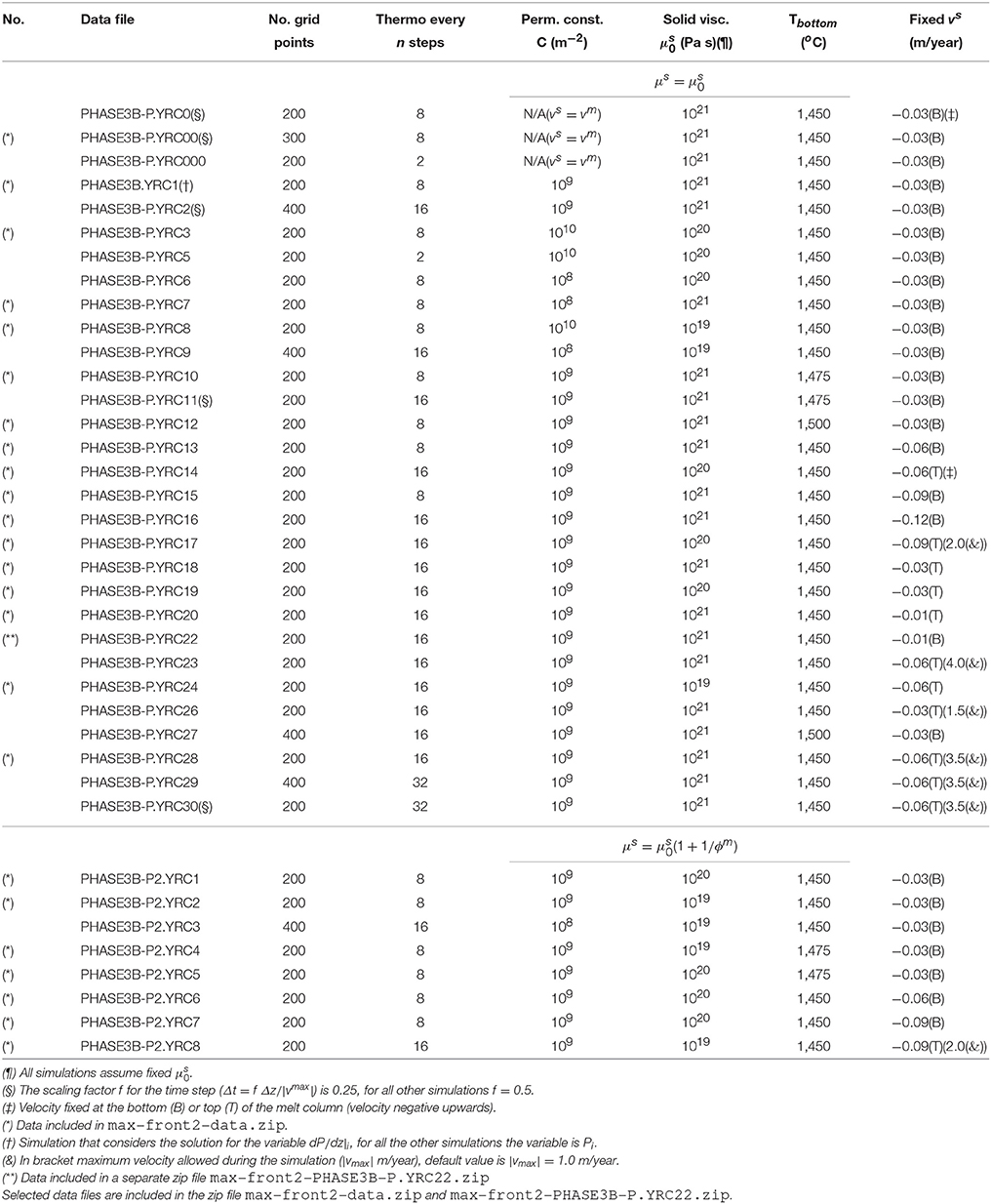
Table 1. List of the dynamic fractional melting simulations (DFM).

The first case assumes a DFM model with v^melt = v^solid. Initial and boundary conditions are equivalent to those applied to the dynamic batch melting model discussed in MF1 (simulation PHASE3-P.BRC4-5), additional details of the new simulation can be found in Table 1 (simulation PHASE3B-P.YRC00). The DEM and DFM models can be considered the closest dynamic equivalent to the batch and fractional melting idea commonly referred in classical petrology. Figure 2 summarizes some of the results. In addition the figure also includes the results of the fractional melting model using the pMELTS version of AlphaMELTS (threshold porosity above which melt is extracted set to 0.005).

FIGURE 2

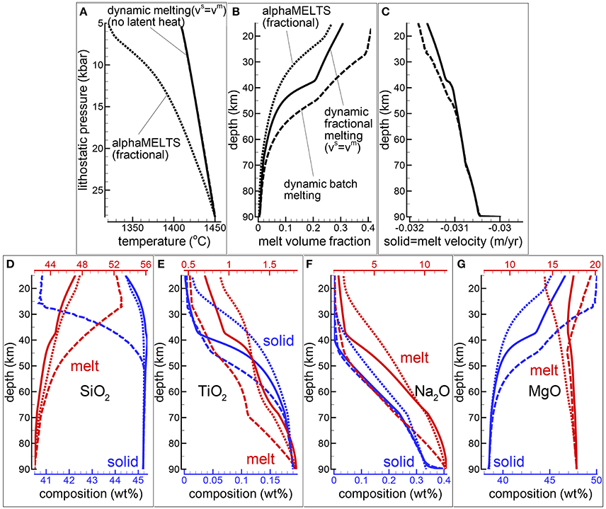
Figure 2. Dynamic melting with v^melt = v^solid. Comparison between dynamic batch melting (dashed lines) and the DFM model with v^melt = v^solid (solid lines). The dynamic batch melting model has been already presented in MF1. The dotted lines show the results for a fractional melting model using AlphaMELTS. For the simulation of the DFM model with v^melt = v^solid, number of grid points nz = 300, number of time steps between two thermodynamic calculations nthermo = 8. (A) Temperature vs. lithostatic pressure, (B) variation of the melt volume fraction with depth, (C) solid and melt velocity, (D–G) composition of the solid and melt (wt %), (D) SiO₂, (E) TiO₂, (F) Na₂O, (G) MgO. The plots show also the composition of the integrated melt (red dotted lines) and the residual solid (dotted blue lines) using AlphaMELTS (pMELTS version). The data file and an animation of the DFM simulation can be downloaded following the instructions in the Supplementary Material (data file PHASE3B-P.YRC00.DAT included in the zip file max-front2-data.zip, movie file mf2-movie1.PHASE3B-P.YRC00.avi).

The difference of the temperature profiles between the DFM model and the fractional melting model with AlphaMELTS (Figure 2A) is mainly due to the contribution of the latent heat of melting, however there is an additional difference between the two models. In the DFM model variable amount of melt is still present in the system at any depth and it affects the thermal profile while with AlphaMELTS only a predefined small mass fraction of melt is always kept with the residual solid. While the net effect of the latent heat on the DFM model in general is difficult to predict, the temperature difference between the DFM model with v^melt = v^solid and AlphaMELTS should represent the largest possible deviation simply because of the large amount of melt involved compared to DFM simulations with separate melt and solid velocities.

Regardless of the type of dynamic model, the total amount of melt at a particular location is the result of the melt transported (melt moving in/out) and the local melt production from the thermodynamic model. In the DFM model with v^melt = v^solid the total melt abundance at a given depth is always less than the amount of melt obtained with the dynamic batch melting model (Figure 2B). It is also not too different from the amount of melt computed by the fractional melting model using AlphaMELTS. The melt volume fraction at a particular depth (or pressure) using AlphaMELTS is given by the sum of the instantaneous volume of melt which is extracted at every point starting from the bottom up to the particular depth.

The larger amount of melt present in the dynamic batch melt model compared with the DFM model with v^melt = v^solid has only a relatively small effect on the increase of the upwelling velocity (Figure 2C). The DFM model with v^melt = v^solid creates melts that are distinctively less rich in silica and with higher TiO₂ content when compared with the melts from the dynamic batch melting model (Figures 2D,E). In the upper portion of the melting column (depth less than ~40 km) the incompatible component Na₂O does not show significant differences in the two models (Figure 2F). The opposite appears to be true for MgO in the same depth range, while at greater depth the MgO content in melt for the two models is very similar (Figure 2G). In the residual solid large differences in the amount of SiO₂ and MgO can be observed at intermediate and low depths (Figures 2D,G). A very small amount of melt crystallizes in sub-system 2 at depths greater than ~60 km but, the solid appears only in the initial stage of the mantle upwelling and it doesn't form any longer after ~2 myr (this solid is not reported in the figure, see the data file PHASE3B-P.YRC00.DAT). An animation illustrating the evolution of the DFM model with v^melt = v^solid over time can be retrieved following the link posted in the Supplementary Material (movie file mf2-movie1.PHASE3B-P.YRC00.avi).

Figure 3 presents a comparison between two 2-phase flow dynamic melting models. One is a DFM model and the other one is the DEM model discussed in the previous study (Figure 4 in MF1, PHASE3-P.YRC4). The conditions imposed to the two models are equivalent, the solid viscosity model is ${\mu }^s={\mu }_0^s$ with ${\mu }_0^s=1e21$ Pa s, the permeability constant is C = 1e9 m⁻², the fixed upwelling velocity at the base of the mantle column is −0.03 m/yr (negative upwards), the mantle bulk composition inside the column at the start of the simulation and at the bottom thorough the duration of the simulation are also the same. The only difference between the two models is how melt chemically interacts with the solid. The DFM model has been solved numerically considering the variables defining the pressure gradient dP/dz and the pressure gradient correction dP′/dz instead of the pressure P and pressure correction P′. The numerical solution obtained using either one of the two solution variables is indistinguishable. The less common application of the pressure gradient may carry some benefits that need to be further investigated (see Appendix 2 in MF1). Additional information about the DFM model can be found in Table 1 (PHASE3B.YRC1). The data file for the DFM model is included in the zip file max-front2-data.zip (see the Supplementary Material for additional information).

FIGURE 3

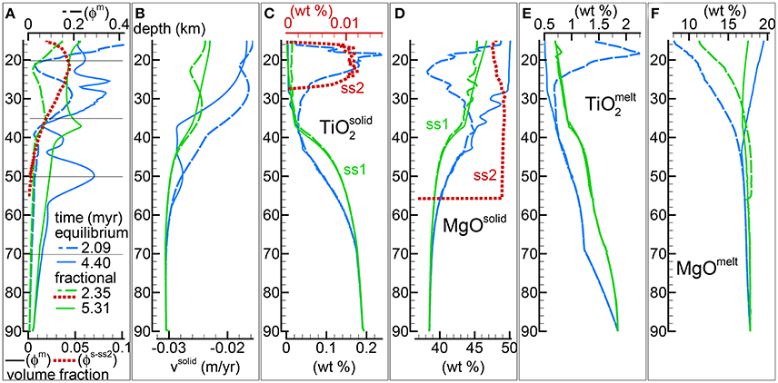
Figure 3. Comparison between dynamic equilibrium melting (DEM) and dynamic fractional melting (DFM). Solid viscosity model: ${\mu }^s={\mu }_0^s$ with ${\mu }_0^s=1e21$ Pa s, permeability constant C = 1e9 m⁻². The equilibrium melting simulation is the same as in Figure 4 of MF1 (data file PHASE3-P.YRC4.DAT, zip file max-front1-data.zip). The data file for the DFM model PHASE3B.YRC1.DAT included in the zip file max-front2-data.zip and an animation (mf2-movie2.PHASE3B.YRC1.avi) can be accessed following the link provided in the Supplementary Material. (A) Melt volume fraction vs. depth at 2 different times (solid and dashed lines). Earliest time is approximately defined for the equilibrium melting model by the first arrival of melt at the top, and approximately by the largest amount of melt reaching the top side for the DFM model. Red dotted line is the volume fraction of solid in sub-system 2 at t ≈ 2.35 myr for the DFM model. The black horizontal lines indicate the depths at which the equilibrium mineralogical assemblage has been computed at 2.35 myr in sub-sys 1 and sub-sys 2 after completing the simulation (Table 2). (B) Velocity of the solid matrix. (C–F) Variation of the solid and melt composition (wt %). (C) TiO₂ in the residual solid, for the DFM model the red dotted line refers to the solid in sub-sys 2 (ss2). (D) MgO in the residual solid, including also the solid in sub-sys 2 for the DFM model (ss2, red dotted line). (E) TiO₂ in melt. (F) MgO in melt.

Selected properties at two different stages of the melt evolution are shown in Figure 3. The earliest stage refers to the time at which in both models a large amount of melt reaches the top side of the column. For the DEM model it corresponds to the first melt arrival, for the DFM model in general this is not always the case and the large melt occurs at a slightly later time (Figure 3A). It is more clearly shown in the data file and later in Figure 8. The properties at a later time illustrate the status of the mantle column when the thermal field does not change significantly any further. As discussed in MF1, melt in this particular DEM model never reaches a time invariant state, but for the DFM model instead the melt distribution approaches a condition close to a steady state.

In general the amount of melt at various depths is lower in the DFM model although this is not always the case since the melt distribution observed in the DEM model varies with time.

Velocity of the mantle at the bottom is fixed at −0.03 m/yr (negative upwards) for the DEM and DFM models. The general behavior of the viscous forces is that they decrease with the increase of the melt content (Equation 8), hence within a zeroth order approximation, this observation provides an interpretation for the overall decrease of the upwelling solid velocity in the upper part where more melt is present (Figure 3B, and also for the next model Figure 4B).

FIGURE 4

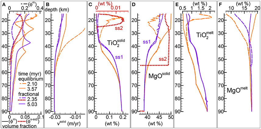
Figure 4. Comparison between the DEM and DFM model with the alternative viscosity model. Solid viscosity model: ${\mu }^s={\mu }_0^s(1+1/{\varphi }^m)$ with ${\mu }_0^s=1e20$ Pa s, permeability constant C = 1e9 m⁻². The equilibrium melting simulation is the same as in Figure 5 of MF1 (data file PHASE3-P2.YRC13.DAT, zip file max-front1-data2.zip). To retrieve the data file for the DFM model PHASE3B-P2.YRC1.DAT included in the zip file max-front2-data.zip see the instructions provided in the Supplementary Material. (A) Melt volume fraction vs. depth at 2 different times (solid and dashed lines). Earliest time is marked by the first arrival of melt at the top for the equilibrium melting, and approximately the largest amount of melt reaching the top side for the DFM model. Red dotted line is the volume fraction of solid in sub-sys 2 at t ≈ 2.35 myr for the DFM model. (B) Velocity of the solid matrix. (C–F) Variation of solid and melt composition (wt %). (C) TiO₂ in the residual solid, also included the solid in sub-sys 2 for the DFM model (ss2, red dotted line). (D) MgO in the residual solid and solid in ss2 for the DFM model. (E) TiO₂ in melt. (F) MgO in melt.

The peculiar feature of the DFM model is the partial crystallization of melt in sub-system 2 (red dotted line in Figure 3A). The amount is relatively small (~ few % in volume) but most importantly it is a transient feature that disappears with time. By comparing the results from various simulations (see the data files and Table 1), it seems that the duration varies depending on the dynamic and thermal conditions imposed to the mantle column.

Figures 3C,D show TiO₂ and MgO in the ss1 and ss2 solid. At the arrival of the large melt volume, the composition of the residual mantle in sub-sys 1 from the two models is quite distinct. In the later stage variation of TiO₂ in the residual solid is not very different in the two models, however MgO shows some significant changes. In the DFM model the composition of the crystallized solid in sub-system 2 varies with depth, in particular it can be noted that TiO₂ is present in the solid only at lower depth. From the data files and following the procedure to determine the bulk composition outlined in the section “Changes in the Thermodynamic Computation”, it is possible to apply AlphaMELTS as a post-processing step at any depth and time to re-compute the equilibrium mineralogical assemblage and the minerals composition that were computed but not recorded during the dynamic simulations. Table 2 illustrates the results after 2.35 myr at four depths indicated by horizontal lines in Figure 3A. It is interesting to note that the solid crystallized in sub-sys 2 is made entirely of olivine except at the lowest depth where a small amount of spinel is also present (hence it explains the rise of TiO₂ in ss2). Table 2 also indicates that at this depth the volume fraction of the liquid and the solid in sub-system 2 are comparable and the residual mantle assemblage in ss1 is made of olivine, ortophyroxene and spinel.

TABLE 2

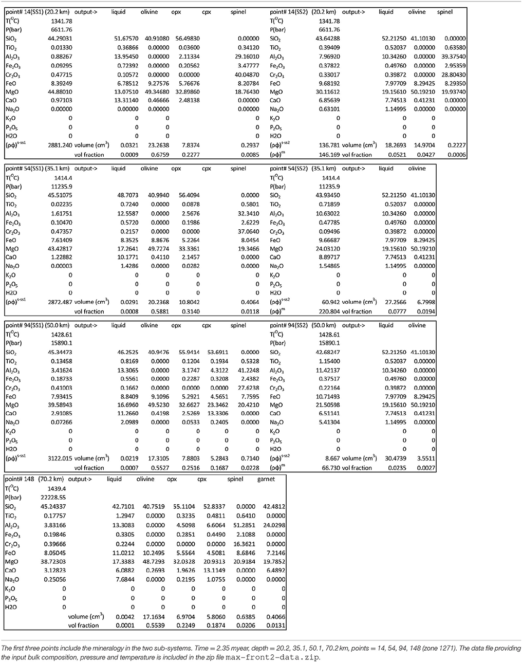
Table 2. Mineral composition and volume fraction at four depths for the DFM model PHASE3B.YRC1 shown in Figures 3–8.

The DEM and DFM models create two series of melt that are compositionally quite dissimilar. Figures 3E,F show an example. An interesting point is that the melt composition in the DFM model is very close to the composition observed in the case that assumed v^melt = v^solid (Figure 2). Inspection of the data file PHASE3B.YRC1.DAT provides additional insight into the compositional variations of other oxides not specifically discussed here.

An animation of the DFM model shown in Figure 3 can be retrieved following the instruction in the Supplementary Material (mf2-movie2.PHASE3B.YRC1.avi).

The second rheology model considered in the previous study (MF1) assumes that the viscosity of the solid is described by a relation that depends also on the melt fraction ${\mu }^s={\mu }_0^s(1+1/{\varphi }^m)$. Figure 4 presents the results of the DFM model with this type of viscosity formulation and a comparison with the DEM model results under similar conditions, ${\mu }_0^s=1e20$ Pa s and permeability constant C = 1e9 m⁻² (DEM model shown also in Figure 5 of MF1, data file PHASE3-P2.YRC13.DAT).

Both DEM and DFM reach a similar steady state in which melt distribution over depth does not significantly change any further over time. In analogy with the observation made for the case that considered the previous viscous model, melt abundance is generally but not always lower in the DFM model compared to the DEM model (Figure 4A). However with the second rheology model the variation of the melt distribution is related to the presence of only one inversion of the gradient of the melt abundance with depth, while the DEM model develops two inversion points. The nature of the inversion has been discussed to some extent in MF1. It should be only mentioned here that the changed behavior is not the result of turning the petrological condition from melting to crystallization but rather the complex effect of the dynamic transport model.

With the DFM model, regardless of the chosen description of the rheology, a second solid crystallizes from the melt in sub-system 2 during the initial stage of the melting process. The melt and solid compositions are similar to those observed with the first viscosity model and they are summarized in Figures 4C–F. The similarity is not entirely unexpected because the net dynamic behavior of the two models is not too different. Even though the value of ${\mu }_0^s=1e20$ Pa s is one order of magnitude lower than the value chosen for the previous viscosity model with ${\mu }^s={\mu }_0^s$, the melt abundance is such that the effective viscosity μ^s becomes very similar in the two cases.

The data file for this DFM model (PHASE3B-P2.YRC1.DATincluded in the zip file max-front2-data.zip) can be retrieved following the instructions in the Supplementary Material.

In the previous study the temperature dependence was not discussed for the DEM model and only two simulations with fixed temperature at the bottom different than 1,450°C were included in the zip data files max-front1-data.zip and max-front1-data2.zip (see Table 1 in MF1). In Figure 5 three simulations of the DFM model are presented assuming similar dynamic and chemical conditions but different temperature at the base of the column, 1,450°C, 1,475°C, and 1,500°C. The DFM model with temperature of 1,450°C is the same shown in Figure 3 (data file PHASE3B.YRC1.DAT). The complete data files of the two simulations with higher temperature are PHASE3B-P.YRC10.DAT (1,475°C) and PHASE3B-P.YRC12.DAT (1,500°C).

FIGURE 5

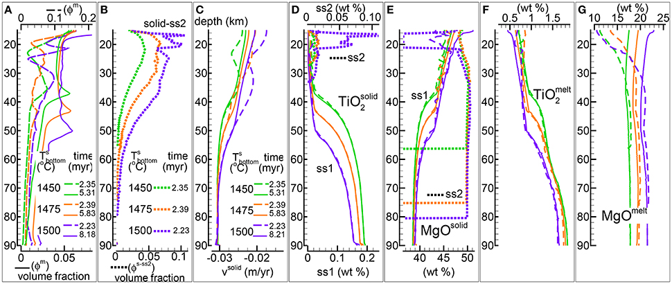
Figure 5. DFM simulations assuming different temperatures at the bottom, 1,450°C (green lines), 1,475°C (orange lines), 1,500°C (purple lines). Solid viscosity model: ${\mu }^s={\mu }_0^s$ with ${\mu }_0^s=1e21$ Pa s, permeability constant C=1e9 m⁻², fixed velocity of the solid at the bottom -0.03 m/yr. (A) Melt volume fraction vs. depth at 2 different times (solid and dashed lines). Earliest time coincides approximately with the largest amount of melt reaching the top side. (B) Volume fraction of solid in sub-sys 2 at the earliest time. (C) Velocity of the solid matrix. (D–G) Variation of the solid and melt composition (wt %). (D) TiO₂ in solid, also the solid in sub-system 2 (ss2, dotted lines). (E) MgO in solid , also the solid in sub-system 2 (ss2, dotted lines). (F) TiO₂ in melt. (G) MgO in melt. The data files can be downloaded following the link provided in the Supplementary Material, zip file max-front2-data.zip, PHASE3B.YRC1.DAT, PHASE3B-P.YRC10.DAT, PHASE3B-P.YRC12.DAT.

In general by increasing the temperature at the bottom larger amount of melt is created inside the mantle column (Figure 5A), but there are additional considerations that can be made. The largest arrival of melt at the top side of the model is not significantly different for the three simulations. However the amount of transient crystallized solid in sub-system 2 increases with the increase of the temperature at the bottom (Figure 5B). In addition the solid in sub-sys 2 begins to form at greater depth when higher temperature is assumed at the bottom. After a variable amount of time all three models reach a steady melt distribution with only one inversion of the melt gradient with depth. The depth of the inversion point is greater for the model with temperature at the bottom set to 1,500°C.

The variations of the velocity of the solid reflect indirectly the different temperatures assumed at the base of the model which have a significant control on the overall melt abundance (Figure 5C).

The compositional difference of the residual mantle (sub-system 1) with temperature is exemplified by TiO₂ and MgO in Figures 5D,E. The behavior does not correlate well, for instance large variations of TiO₂ can be observed as the depth increases (>35 km) while the largest variations of MgO occur between ~60 and ~35 km depth. The melt composition does show some dependence on the temperature in particular for the MgO content (Figures 5F,G). The variation is less pronounced for Na₂O and Cr₂O₃ and it occurs mostly at depths greater than ~35–50 km (plots of these oxides is not included in Figure 5). The data files provide a complete overview of the solid and mantle composition.

An animation of the simulation with temperature at the bottom set to 1,500°C (mf2-movie3.PHASE3B-P.YRC12.avi) is available following the link provided in the Supplementary Material.

A systematic study on the effect of the imposed velocity of the mantle at the boundary (either top or bottom) was also not addressed previously in MF1. Fixing the velocity at the top or bottom boundary may seem a minor detail, after all the total length of the mantle column is only 75 km. From a conceptual point of view the two different conditions describe, at least approximately in 1-D, either passive flow, a regime in which pulling forces (e.g., subducting slab) control the mantle upwelling, or alternatively active flow that could be the result of thermochemical buoyancy (e.g., rising plume).

Figure 6 summarizes some of the results of four DFM simulations that assume different velocities at the bottom ranging from −0.01 to −0.09 m/yr (negative upwards) while all the other parameters and conditions are kept unchanged. The complete data files are available (see the Supplementary Material), PHASE3B-P.YRC15.DAT (−0.09 m/yr) PHASE3B-P.YRC13.DAT (−0.06 m/yr), PHASE3B.YRC1.DAT (−0.03 m/yr) included in max-front2-data.zip. The data file PHASE3B-P.YRC22.DAT (−0.01 m/yr) is included separately in max-front2-PHASE3B-P.YRC22.zip. Additional information is provided in Table 1.

FIGURE 6

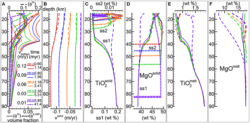
Figure 6. DFM simulations assuming a different velocity of the solid at the bottom (negative upwards), −0.12 m/yr (red lines), −0.09 m/yr (blue lines), −0.06 m/yr (green lines), −0.03 m/yr (orange lines), −0.01 m/yr (purple lines). Solid viscosity model: ${\mu }^s={\mu }_0^s$ with ${\mu }_0^s=1e21$ Pa s, permeability constant C = 1e9 m⁻², temperature at the bottom 1,450°C. (A) Melt volume fraction vs. depth at 2 different times (solid and dashed lines). Earliest time indicates approximately the largest amount of melt reaching the top side. Dotted line is the volume fraction of solid in sub-system 2. (B) Velocity of the solid matrix. (C–F) Variation of solid and melt composition (wt %). (C) TiO₂ in the residual solid (ss1) and solid in sub-sys 2 (ss2, dotted lines). (D) MgO in the residual solid (ss1) and solid in sub-sys 2 (ss2, dotted lines). (E) TiO₂ in melt. (F) MgO in melt. Data files included in the zip file max-front2-data.zip, PHASE3B.YRC1.DAT (−0.03 m/yr), PHASE3B-P.YRC13.DAT (−0.06 m/yr), PHASE3B-P.YRC15.DAT (−0.09 m/yr). Data file PHASE3B-P.YRC22.DAT (−0.01 m/yr) is included separately. See the Supplementary Material for additional information.

Perhaps the most interesting observation involves the simulation with the smaller upwelling velocity imposed at the base (−0.01 m/yr) that somehow stands out compared to the others. The amount of crystallized solid in sub-system 2 is significantly lower (Figure 6A), it also appears at far greater depth (>80 km) and it is persistent for much longer time than for all the other models. The steady state melt distribution includes an inversion point that is much less pronounced than in the other simulations, although it occurs at similar depth (~35–38 km). The mantle velocities inside the simulation colum are in direct relation with the imposed velocity at the base (Figure 6B). From Figures 6C–F it is also quite evident that the composition of the melt and residual solid when the largest first melt reaches the top side are remarkably different. The composition of the solid mantle at later time becomes more similar to the composition observed in the other simulations, all being very similar. For the melt instead, the composition remains still noticeably distinct from the other models. The difference also appears for oxides not shown in the figure but accessible through the data file, for example Al₂O₃ and CaO, in particular at lower depths.

In the previous study (MF1) only one numerical model was carried out assuming a fixed velocity of the mantle on the top side of the mantle column (Table 1 in MF1) and the results were not discussed. With the DFM model few more simulations with this type of boundary condition have been carried out (Table 1). Figure 7 compares the results of a simulation discussed earlier PHASE3B.YRC1 (Figures 3, 5, 6) that assumes a fixed velocity at the bottom (−0.03 m/yr, μ^s = 1e21 Pa s) and two numerical models in which the same constant velocity is imposed on the top side instead. These last two differ in the setup of the solid viscosity parameter μ^s that is 1e20 and 1e21 Pa s (data files PHASE3B-P.YRC19.DAT, PHASE3B-P.YRC18.DAT).

FIGURE 7

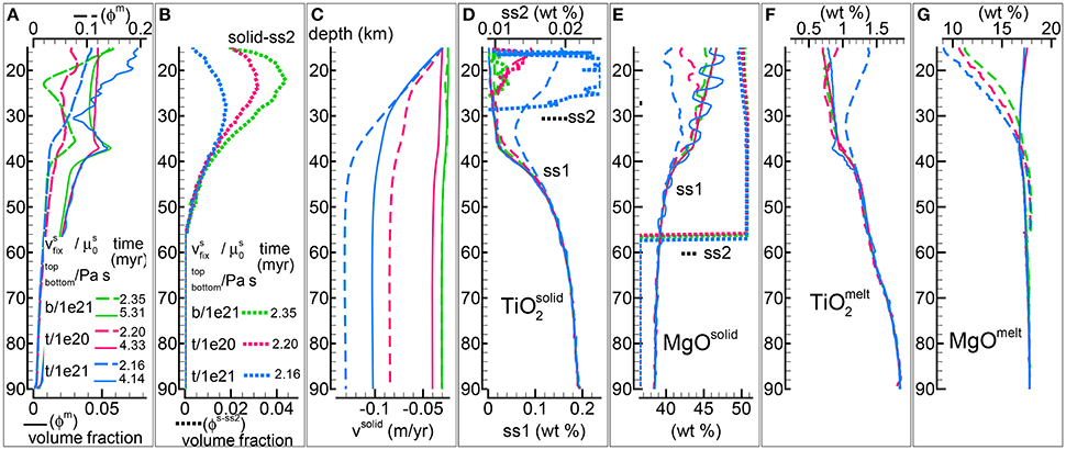
Figure 7. DFM model assuming fixed velocity of the solid (−0.03 m/yr) at the top (t) or the bottom (b). Fixed velocity at the bottom with ${\mu }_0^s=1e21$ Pa s (green lines, same as in Figures 3, 5, 6), fixed velocity at the top with ${\mu }_0^s=1e20$ Pa s (magenta lines), fixed velocity at the top with ${\mu }_0^s=1e21$ Pa s (blue lines) Solid viscosity model: ${\mu }^s={\mu }_0^s$, permeability constant C = 1e9 m⁻².(A) Melt volume fraction vs. depth at 2 different times (solid and dashed lines). Earliest time is approximately defined by the largest amount of melt reaching the top side. Dotted line is the volume fraction of solid in sub-sys 2. (B) Velocity of the solid matrix. (C–F) Compositional variations in solid and melt (wt %). (C) TiO₂ in the residual solid (ss1) and solid in sub-sys 2 (ss2, dotted lines). (D) MgO in the residual solid (ss1) and solid in sub-sys 2 (ss2, dotted lines). (E) TiO₂ in melt. (F) MgO in melt. Data files PHASE3B.YRC1.DAT (bottom fixed, ${\mu }_0^s=1e21$ Pa s), PHASE3B-P.YRC19.DAT (top fixed, ${\mu }_0^s=1e20$ Pa s), PHASE3B-P.YRC18.DAT (top fixed, ${\mu }_0^s=1e21$ Pa s) are included in the zip file max-front2-data.zip. See the Supplementary Material for additional information.

The first observation that can be made is that the large first melt arrival on the top side is smaller when the mantle velocity is fixed on this side of the model (Figure 7A, dashed lines). The amount of crystallized solid in sub-system 2 is also smaller with the top velocity fixed, although the depth of the first appearance of the solid in ss2 (~56 km) is practically the same for the three cases considered (Figure 7B).

The melt distribution at later time is very similar for the model with fixed velocity at the bottom and viscosity = 1e21 Pa s and the simulation with fixed velocity at the top and viscosity = 1e20 Pa s (Figure 7A, green and red solid lines). The other simulation with fixed top velocity but viscosity = 1e21 Pa s shows instead larger melt variation at lower depths (Figure 7A, blue solid line). Perhaps the most important feature of this simulation is that the melt distribution, in particular in the upper portion of the mantle column is extremely variable over time. This characteristic behavior is not quite evident from Figure 7 but it is clear by inspecting the data file and from the animation that can be retrieved following the link provided in the Supplementary Material (mf2-movie4.PHASE3B-P.YRC18.avi).

Figure 7C shows the significant increase of the mantle velocity with depth for the models with fixed velocity on the top side. It should be mentioned that for the model with a transient melt distribution, the velocity of the solid also varies over time inside the mantle column.

When the velocity at the top is kept fixed, the composition of the residual mantle (sub-system 1) appears to be quite different at lower depths (≲40 km) (Figures 7D,E). The model that does not reach a steady state develops temporal and spatial variations of the MgO content at low depths.

In the earlier stage the melt composition shows some variability among the three models (Figures 7F,G). Moving forward in time these differences tend to disappear for two of them, however significant variations of the melt composition are observed for the unsteady model.

The model with fixed velocity on the top side that exhibits large temporal and spatial variations of the dynamic and petrological properties has been tested quite extensively by running several simulations varying the number of spatial grid points, time step, maximum velocity allowed in the model and time interval between thermodynamic computations (Table 1). All these test simulations seem to confirm the conclusion that, at the conditions imposed on the model, the unsteady behavior is not the result of a spurious numerical artifact.

Because in MF1 the effect of the location of the fixed boundary velocity was not properly discussed for the DEM model, the Appendix presents the results of two new DEM simulations that assume fixed velocity of the solid, one at the top and the other at the bottom side of the mantle column.

As in the previous study, the variations of some of the results over time at the point of extraction (exit point or top side of the model) are briefly illustrated here. Selected DFM simulations from those presented earlier assuming the viscosity model ${\mu }^s={\mu }_0^s$ are considered in Figure 8. In addition results of the dynamic batch melting from the previous study and DFM with v^m = v^s are also plotted. Figure 8A illustrates the amount of melt extracted per unit of time. The largest melt flux is observed for the model with the largest velocity of the solid imposed at the bottom (blue line). The earliest arrival of the melt at the exit point is consistent with the large upwelling velocity of the solid and the melt (Figure 8B). The second largest flux (purple line) is the result of the high temperature at the bottom (1,500°C) that generates large amount of melt. Periodic oscillations over time are created by the model with solid velocity fixed at the top side and solid viscosity μ^s = 1e21 Pa s. These temporal variations are not only evident in the melt flux and melt velocity but also in the melt composition (Figures 8C,D). Other simulations instead seem to approach the composition of the DFM model with v^m = v^s, but only when the model assumes the same fixed temperature at the bottom (1,450°C). Once the formation of the second solid in sub -system 2 ceased, starting at the point indicated by an arrow in Figure 8D, the composition of the melt products afterwards seems to be affected to some extent. The complete data sets related to these models are PHASE3-P.BRC4-5.DAT (zip file max-front1-data.zip in MF1), PHASE3B-P.YRC00.DAT (DFM with v^m = v^s), PHASE3B.YRC1.DAT (green line), PHASE3B-P.YRC15.DAT (blue line), PHASE3B-P.YRC12.DAT (purple line) PHASE3B-P.YRC19.DAT (magenta line), PHASE3B-P.YRC18.DAT (black dotted line) (zip file max-front2-data.zip this study).

FIGURE 8

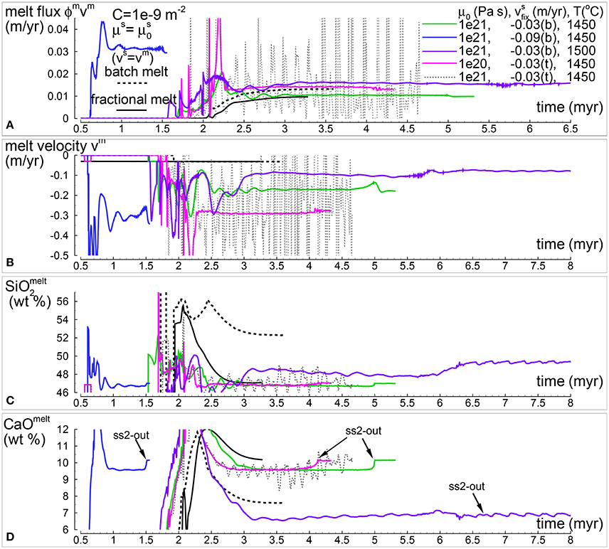
Figure 8. Temporal variation of selected melt properties at the top side of the simulation for three models with ${\mu }^s={\mu }_0^s$, and permeability constant C = 10⁻⁹ m⁻². Different lines correspond to simulations with different ${\mu }_0^s$, velocity of the solid at the top (t) or bottom (b) and/or different temperature. Results from the batch melting model presented in the previous paper (MF1) and DFM with v^s = v^m are also included. (A) Melt flux (ϕ^mv^m), amount of melt per year that is extracted from the melt column. (B) Melt velocity (m/yr). (C) Melt composition: SiO₂ (wt %). (D) Melt composition: CaO (wt %). Complete data can be found in PHASE3-P.BRC4-5.DAT (batch melt v^s = v^m, zip file max-front1-data.zip in MF1), PHASE3B-P.YRC00.DAT (fractional melt v^s = v^m, black line), PHASE3B.YRC1.DAT (green line), PHASE3-P.YRC15.DAT (blue line), PHASE3B-P.YRC12.DAT (purple line), PHASE3B-P.YRC19.DAT (magenta line) and PHASE3B-P.YRC18.DAT (dotted black line) (all data included in the zip file max-front2-data.zip).

Fewer simulations involving the DFM model have been carried out with the second viscosity model ${\mu }^s={\mu }_0^s(1+1/{\varphi }^m)$ (Table 1). Figure 9 includes the results at the point of extraction for the model shown in Figure 4 PHASE3B-P2.YRC1.DAT (purple lines) along with two other simulations not discussed previously, one with the same reference viscosity ${\mu }_0^s=1e20$ Pa s but higher velocity at the bottom (−0.09 m/yr) PHASE3-P2.YRC7.DAT (red lines), and the second one with lower viscosity ${\mu }_0^s=1e20$ Pa s and fixed velocity on the top side (-0.09 m/yr) PHASE3B-P2.YRC8.DAT (green lines) (all data included in the zip file max-front2-data.zip). Batch melting from MF1 and the DFM with v^m = v^s are also included for comparison. As expected the models with higher solid velocity, either at the top or the bottom, generate larger melt flux (Figure 9A). The one with the imposed solid velocity on the top side develops the fastest melt transport (Figure 9B). From a compositional point of view, once the models reach approximately a condition of steady state and the solid in sub-system 2 does not crystallize anymore, they all seem to approach the composition of the melt found by the DFM model with v^m = v^s (Figures 9C,D).

FIGURE 9

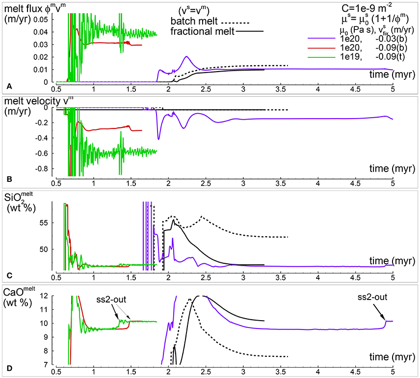
Figure 9. Temporal variation of selected melt properties at the top side of the simulation for three models with ${\mu }^s={\mu }_0^s(1+1/{\varphi }^m)$, permeability constant C = 10⁻⁹ m⁻² and temperature at the bottom T = 1,450°C. Different lines correspond to simulations with different ${\mu }_0^s$ and velocity of the solid at the top (t) or bottom (b). For comparison simulations of the batch melting model (introduced in the previous study, MF1) and DFM with v^s = v^m are also included. (A) Melt flux (ϕ^mv^m). (B) Melt velocity (m/yr). (C) Melt composition: SiO₂ (wt %). (D) Melt composition: CaO (wt %). Complete data can be found in PHASE3-P.BRC4-5.DAT (batch melt v^s = v^m, zip file max-front1-data.zip in MF1), PHASE3B-P.YRC00.DAT (fractional melt v^s = v^m, black line), PHASE3B-P2.YRC1.DAT (purple lines), PHASE3-P2.YRC7.DAT (red lines), and PHASE3B-P2.YRC8.DAT (green lines) (all data included in the zip file max-front2-data.zip).

Discussion and Conclusions

The simplest and possibly the most general description of dynamic melting under the condition of chemical disequilibrium between the residual solid and the local melt has been developed for this study. The previous section presented some of the results of this model that has been referred as dynamic fractional melting (DFM). Many of these results will require further analysis, particularly for a comparison with real petrological data. Only a simple observation is made here regarding the crystallization of a second solid which consists essentially of olivine. The results from the DFM model suggest a possible mechanism for the formation of dunite melt channels found in several ophiolites (e.g., Kelemen et al., 1995; Suhr, 1999; Godard et al., 2000; Müntener and Piccardo, 2003; Morgan et al., 2008; Abily and Ceuleneer, 2013).

A comparison with the dynamic equilibrium melting (DEM) introduced in the previous study (MF1) highlighted the main differences between the two models. The effect on the DFM process of the fixed bottom temperature, upwelling mantle velocity at the top or bottom side of the mantle column have been investigated in some detail.

Summarizing some of the findings, the first observation that can be made is that with the DFM model the amount of melt distributed inside the model is often but not always less than the amount obtained with the DEM model. The residual solid and the melt compositions are quite distinctive in the two models. In most cases the unique presence of a second solid in sub-system 2 is a transient feature of the DFM model during the initial stage of the melt evolution. The differences between the DFM and DEM model appear to be persistent regardless of the chosen description of the solid mantle rheology.

In general there is a positive correlation between the temperature at the base of the mantle column and the amount of melt inside the DFM model. The inversion point of the melt gradient, a feature that has been found also in the previous study, appears at greater depth. The composition of the melt and solid are affected by the temperature change but there is no clear predictive pattern to the variations with depth and time.

Considering different values for the fixed upwelling velocity of the solid mantle at the base of the model (active flow), the results obtained with the lowest velocity that was assumed in this study (−0.01 m/yr, negative upwards) somehow deviate from the general behavior observed in DFM models with higher imposed upwelling velocities. In particular this is quite evident for the melt abundance, melt and solid composition in the two sub-systems when the first melt reaches the top side of the model and melt composition at later times.

Although the depth range of the mantle column is rather limited (75 km), the definition of the boundary fixed velocity of the mantle at the top or the bottom side (passive/active flow) has an effect on the DFM process. In particular, under certain conditions, by imposing a fixed velocity on the top side (passive flow), the melt shows large temporal and spatial variations which are not observed when the same velocity is assumed at the bottom side (active flow).

The travel time, flux and composition of the melt at the extraction point (top side of the model) depend on various mantle conditions such as the bottom temperature, imposed upwelling velocity of the solid (either on the top or bottom side), and rheological properties.

Even though the DEM and DFM models allow us to explore the evolution of mantle melting in time and space, they can still be considered simplified representations of the melting process. Some of the limitations have been outlined earlier. The thermodynamic model carries its own limitations which were extensively investigated in a series of studies (Hirschmann et al., 1998, 1999a,b; Asimow et al., 2001) addressing the earlier version of the melt model (Ghiorso and Sacks, 1995). The newer version used in this study and in MF1 was better calibrated for melting of mantle rocks (pMELTS, Ghiorso et al., 2002), nevertheless some discrepancies with experimental data could not have been avoided (e.g., error on the MgO content in melt is ~1–4%).

One point that perhaps deserve a further consideration is the composition of the solid mantle source. There is a lot of debate regarding the presence of an eclogitic or component contributing to the mantle melt products (e.g., Ito and Mahoney, 2005a,b; Strake and Bourdon, 2009; Brown and Lesher, 2014; Shorttle et al., 2014; Lambart et al., 2016). It has clear repercussions on our understanding of the petrology of the deep Earth Interior (e.g., Allègre and Turcotte, 1986; Hauri, 1996; Sobolev et al., 2005; Barker et al., 2014; Elkins et al., 2016). From a modeling perspective it won't be difficult to assume a local system at the bottom of the melt column that is made of a weighted average of a peridotitic and eclogitic component. More interesting would be to assume instead that two distinct lithologies coexist in a predefined volumetric proportion, each forming a separate sub-system in chemical equilibrium. This last scheme would be still approachable but one problem that would clearly emerge is how to treat the melt product(s). Once one of the two sub-systems creates some melt or both of them separately create some melt, if some kind of fractional melting similar to the one described in this work is imposed, then some assumptions need to be made on how the melt product(s) will be transferred into a third or fourth sub-system where it/they will mix with all the previous melt products. Perhaps even more challenging is the case of equilibrium melting because, for example, when two melts are present within the same local volume, they may or may not mix and they may or may not equilibrate (together or separately) with one or both lithologies.

Despite the fact that these conceptual ideas can be modeled numerically, it is not known yet whether they can be associated to some realistic melting process or they are nothing more than numerical exercises. There is one additional complication that discourage (at least the author of this study) from pursuing this type of melt modeling for complex petrological assemblages. The characterization of the eclogitic component in the mantle at the present time is based on indirect evidences. There is no understanding of the level of chemical equilibration between eclogite and peridotite in the mantle nor the physical distribution of the two assemblages (Tirone et al., 2015). Only a combination of specific experimental studies to determine the kinetics of the chemical equilibration in combination with large scale geodynamic modeling could provide at least some information on this issue. Unfortunately for various reasons it seems that this type of study will not materialize anytime soon.

Regardless of the above considerations, the DEM and DFM models can be used to try to interpret real petrological data. However for a petrologist using geochemical data a dynamic-thermodynamic model may not always be an absolute necessity. A thermodynamic study using for example alphaMELTS should be sufficient to gain some general idea about the temperature/pressure and composition of the source at the beginning of a melting process when it is driven by mantle upwelling. This is quite reasonable in particular if the “true” melting process can be related to the DEM model. In this case often (but not always) the dynamic evolution does not affect significantly the composition of the melt at the top of the mantle column which depends essentially on the initial conditions of the mantle. Any further interpretation that involves temporal and spatial variations of melt abundance and composition would require some model similar to the one in this study provided that the petrological/thermodynamic description is sufficiently accurate. In terms of the procedure that should be followed, there is no easy shortcut or simple formula/tool that can be applied for the task. A possible course of action could be the following. If the petrological data consist only of melt composition on lavas or intrusive components, then plots similar to Figures 8, 9 could be used with the available simulation data to provide a first assessment. Since the exit point is located at 15 km depth (5 kbar), it may be necessary to revise the numerical results or correct the observed melt composition for partial crystallization that may have occurred at lower depths. If samples from the mantle are also available then other plots showing variations of the certain properties with depth may turn to be useful for a direct comparison. When few of the chemical or mineralogical components do not match the real data then it may be necessary to revise the starting mantle composition chosen in this and the previous study, and new numerical simulations would be needed. Petrological data alone may not be sufficient to put a firm constraint on the temporal and dynamic nature of the melting process and more information should be included in the study. Geophysical data, for example seismic, gravimetric, electrical conductivity, could be helpful to constrain the variation of the melt distribution and/or the variation of the thermal state with depth. For this reason it would be easier to apply the DEM or DFM models to present day or recent magmatic events. Geochronological data could also provide support to bracket the temporal window of the melting process and perhaps the volumetric distribution over time.

One important contribution has been left out of the discussion describing the melting process so far, that is the presence of water. It will be the main topic of the third and last installment on modeling dynamic melting in the mantle.

Author Contributions

The author confirms being the sole contributor of this work and approved it for publication.

Conflict of Interest Statement

The author declares that the research was conducted in the absence of any commercial or financial relationships that could be construed as a potential conflict of interest.

Acknowledgments

The editor (Paterno Castillo) was instrumental in assisting the author during the review process of this and the previous study (MF1). The comments and advice from two reviewers were greatly appreciated, they significantly helped to improve the clarity of the manuscript. Thanks to Jan Sessing for developing the preliminary version of the program used in this study for a petrology project while pursuing his MS degree at the Ruhr-Universität Bochum, Institut für Geologie, Mineralogie und Geophysik. Part of the manuscript was prepared at the Department of Mathematics and Geosciences, University of Trieste, Italy. Tina's support thorough all this journey will not be forgotten.

Supplementary Material

The Supplementary Material for this article can be found online at: https://www.frontiersin.org/articles/10.3389/feart.2018.00018/full#supplementary-material

All the data of the simulations for this study can be downloaded from figshare following the link provide in the supplementary material file https://figshare.com/collections/max-front2/3745487

References

Abily, B., and Ceuleneer, G. (2013). The dunitic mantle-crust transition zone in the Oman ophiolite: residue of melt-rock interaction, cumulates from high-MgO melts, or both? Geology 41, 67–70. doi: 10.1130/G33351.1

CrossRef Full Text | Google Scholar

Allègre, C. J., and Turcotte, D. L. (1986). Implications of a two-component marble-cake mantle. Nature 323, 123–127. doi: 10.1038/323123a0

CrossRef Full Text | Google Scholar

Asimow, P. D. (2002). Steady state mantle-melt interaction in one dimension: II. Thermal interactions and irreversible terms. J. Petrol. 43, 1707–1724. doi: 10.1093/petrology/43.9.1707

CrossRef Full Text | Google Scholar

Asimow, P. D., Hirschmann, M. M., and Stolper, E. M. (2001). Calculation of peridotite partial melting from thermodynamic models of minerals and melts: IV. Adiabatic decompression and the composition and mean properties of mid-ocean ridge basalts. J. Petrol. 42, 963–998. doi: 10.1093/petrology/42.5.963

CrossRef Full Text | Google Scholar

Asimow, P. D., and Stolper, E. M. (1999). Steady-state mantle-melt interactions in one dimension: I. Equilibrium transport and melt focusing. J. Petrol. 40, 475–494. doi: 10.1093/petroj/40.3.475

CrossRef Full Text | Google Scholar

Barker, A. K., Holm, P. M., and Troll, V. R. (2014). The role of eclogite in the mantle heterogeneity at Cape Verde. Contrib. Mineral. Petrol. 168, 1052. doi: 10.1007/s00410-014-1052-0

CrossRef Full Text | Google Scholar

Bercovici, D., and Ricard, Y. (2003). Energetics of a two-phase model of lithospheric damage, shear localization and plate boundary formation. Geophys. J. Int. 152, 581–596. doi: 10.1046/j.1365-246X.2003.01854.x

CrossRef Full Text | Google Scholar

Bercovici, D., Ricard, Y., and Schubert, G. (2001). A two-phase model for compaction and damage, part 1: general theory. J. geophys. Res. 106, 8887–8906. doi: 10.1029/2000JB900430

CrossRef Full Text | Google Scholar

Brown, E. L., and Lesher, C. E. (2016). REEBOX PRO: a forward model simulating melting of thermally and lithologically variable upwelling mantle. Geochem. Geophys. Geosyst. 17, 3929–3968. doi: 10.1002/2016GC006579

CrossRef Full Text | Google Scholar

Brown, E. L., and Lesher, C. E. (2014). North Atlantic magmatism controlled by temperature, mantle composition and buoyancy. Nat. Geosci. 7, 820–824. doi: 10.1038/ngeo2264

CrossRef Full Text | Google Scholar

Carr, M. J., and Gazel, E. (2017). Igpet software for modeling igneous processes: examples of application using the open educational version. Miner. Petrol. 11, 283–289. doi: 10.1007/s00710-016-0473-z

CrossRef Full Text | Google Scholar

Elkins, L. J., Scott, S. R., Sims, K. W. W., Rivers, E. R., Devey, C. W., Reagan, M. K., et al. (2016) Exploring the role of mantle eclogite at mid-ocean ridges hotspots: U-series constraints on Jan Mayen Island the Kolbeinsey Ridge. Chem. Geol. 444, 128–140. doi: 10.1016/j.chemgeo.2016.09.035

CrossRef Full Text | Google Scholar

Ghiorso, M. S. (1985). Chemical mass transfer in magmatic processes I. thermodynamic relations and numerical algorithms. Contrib. Mineral. Petrol. 90, 107–120. doi: 10.1007/BF00378254

CrossRef Full Text | Google Scholar

Ghiorso, M. S., and Sack, R. O. (1995). Chemical mass transfer in magmatic processes IV. a revised and internally consistent thermodynamic model for the interpolation and extrapolation of liquid-solid equilibria in magmatic systems at elevated temperatures and pressures. Contrib. Mineral. Petrol. 119, 197–212. doi: 10.1007/BF00307281

CrossRef Full Text | Google Scholar

Ghiorso, M. S., Hirschmann, M. M., Reiners, P. W., and Kress, V. C. III. (2002). The pMELTS: a revision of MELTS for improved calculation of phase relations and major element partitioning related to partial melting of the mantle to 3 GPa. Geochem. Geophys. Geosys. 5:1030. doi: 10.1029/2001GC000217

CrossRef Full Text | Google Scholar

Ghods, A., and Arkani-Hamed, J. (2000). Melt migration beneath mid-ocean ridges. Geophys. J. Int. 140, 687–697. doi: 10.1046/j.1365-246X.2000.00032.x

CrossRef Full Text | Google Scholar

Godard, M., Jousselin, D., and Bodinier, J. L. (2000). Relationships between geochemistry and structure beneath a palaeo-spreading centre: a study of the mantle section in the Oman ophiolite. Earth Planet. Sci. Lett. 180, 133–148. doi: 10.1016/S0012-821X(00)00149-7

CrossRef Full Text | Google Scholar

Hauri, E. H. (1996). Major-element variability in the Hawaiian mantle plume. Nature 382, 415–419. doi: 10.1038/382415a0

CrossRef Full Text | Google Scholar

Herzberg, C., and Asimow, P. D. (2008). Petrology of some oceanic island basalts: PRIMELT2.xls software for primary magma calculation. Geochem. Geophys. Geosyst. 9:Q09001. doi: 10.1029/2008GC002057

CrossRef Full Text | Google Scholar

Hewitt, I. J. (2010). Modelling melting rates in upwelling mantle. Earth Planet. Sci. Lett. 300, 264–274. doi: 10.1016/j.epsl.2010.10.010

CrossRef Full Text | Google Scholar

Hewitt, I. J., and Fowler, A. C. (2008). Partial melting in an upwelling mantle column. Proc. Roy. Soc. A 464, 2467–2491. doi: 10.1098/rspa.2008.0045

CrossRef Full Text | Google Scholar

Hirschmann, M. M., Asimow, P. D., Ghiorso, M. S., and Stolper, E. M. (1999a). Calculation of peridotite partial melting from thermodynamic models of minerals and melts. III. Controls on isobaric melt production and the effect of water on melt production. J. Petrol. 40, 831–851. doi: 10.1093/petroj/40.5.831

CrossRef Full Text | Google Scholar

Hirschmann, M. M., Ghiorso, M. S., and Stolper, E. M. (1999b). Calculation of peridotite partial melting from thermodynamic models of minerals and melts. II. Isobaric variations in melts near the solidus and owing to variable source composition. J. Petrol. 40, 297–313. doi: 10.1093/petroj/40.2.297

CrossRef Full Text | Google Scholar

Hirschmann, M. M., Ghiorso, M. S., Asimow, P. D., Wasylenki, L. E., and Stolper, E. M. (1998). Calculation of peridotite partial melting from thermodynamic models of minerals and melts. I. Review of methods and comparison with experiments. J. Petrol. 39, 1091–1115. doi: 10.1093/petroj/39.6.1091

CrossRef Full Text | Google Scholar

Hole, M. J. (2015). The generation of continental flood basalts by decompression melting of internally heated mantle. Geology 43, 311–314. doi: 10.1130/G36442.1

CrossRef Full Text | Google Scholar

Katz, R. F. (2008). Magma dynamics with the enthalpy method: benchmark solutions and magmatic focusing at mid-ocean ridges. J. Petrol. 49, 2099–2121. doi: 10.1093/petrology/egn058

CrossRef Full Text | Google Scholar

Kelemen, P. B., Shimizu, N., and Salters, V. J. M. (1995). Extraction of mid-ocean-ridge basalt from the upwelling mantle by focused flow of melt in dunite channels. Nature 375, 747–753. doi: 10.1038/375747a0

CrossRef Full Text | Google Scholar

Ito, G., and Mahoney, J. (2005a). Flow and melting of a heterogeneous mantle: 1. Importance to the geochemistry of ocean island and mid-ocean ridge basalts. Earth Planet. Sci. Lett. 230, 29–46. doi: 10.1016/j.epsl.2004.10.035

CrossRef Full Text | Google Scholar

Ito, G., and Mahoney, J. (2005b). Flow and melting of a heterogeneous mantle: 2. Implications for a non-layered mantle. Earth Planet. Sci. Lett. 230, 47–63. doi: 10.1016/j.epsl.2004.10.034

CrossRef Full Text | Google Scholar

Lambart, S., Baker, M. B., and Stolper, E. M. (2016). The role of pyroxenite in basalt genesis: melt-PX, a melting parameterization for mantle pyroxenites between 0.9 and 5?GPa. J. Geophys. Res. 121, 5708–5735. doi: 10.1002/2015JB012762

CrossRef Full Text | Google Scholar

Langmuir, C. H., Klein, E. M., and Plank, T. (1992). “Petrological systematics ofMid-ocean ridge basalts: constraints on melt generation beneath ocean ridges,” in Mantle Flow and Melt Generation at Mid-Ocean Ridges, Geophysical Monograph 71, eds J. P. Morgan, D. K. Blackman, and J. M. Sinton (Washington, DC: American Geophysical Union), 183–280.

McKenzie, D. (1984). The generation and compaction of partially molten rock. J. Petrol. 25, 713–765. doi: 10.1093/petrology/25.3.713

CrossRef Full Text | Google Scholar

Morgan, Z., Liang, Y., and Kelemen, P. (2008). Significance of the concentration gradients associated with dunite bodies in the Josephine and Trinity ophiolites. Geochem. Geophys. Geosyst. 9:Q07025. doi: 10.1029/2008GC001954

CrossRef Full Text | Google Scholar

Müntener, O., and Piccardo, G. B. (2003). Melt migration in ophiolitic peridotites: the message from Alpine-Apennine peridotites and implications for embryonic ocean basins. Geol. Soc. London Spec. Publ. 218, 69–89. doi: 10.1144/GSL.SP.2003.218.01.05

CrossRef Full Text

Oliveira, B., Afonso, J. C., Zlotnik, S., and Diez, P. (2018). Numerical modelling of multiphase multicomponent reactive transport in the Earth's interior. Geophys. J. Int. 212, 345–388. doi: 10.1093/gji/ggx399

CrossRef Full Text | Google Scholar

Rey, P. F. (2015). The geodynamics of mantle melting. Geology 43, 367–368. doi: 10.1130/focus042015.1

CrossRef Full Text | Google Scholar

Richardson, C. N. (1998). Melt flow in a variable viscosity matrix. Geophys. Res. Lett. 25, 1099–1102. doi: 10.1029/98GL50565

CrossRef Full Text | Google Scholar

Rudge, J. F., Bercovici, D., and Spiegelman, M. (2011). Disequilibrium melting of a two phase multicomponent mantle. Geophys. J. Int. 184, 699–718. doi: 10.1111/j.1365-246X.2010.04870.x

CrossRef Full Text | Google Scholar

Schmeling, H. (2000). “Partial melting and melt segregation in a convecting mantle,” in Physics and Chemistry of Partially Molten Rocks, eds N. Bagdassarov, D. Laporte, and A. B. Thompson (Dordrecht: Kluwer), 141–178.

Google Scholar

Scott, D. R., and Stevenson, D. J. (1986). Magma ascent by porous flow. J. Geophys. Res. 91, 9283–9296. doi: 10.1029/JB091iB09p09283

CrossRef Full Text | Google Scholar

Scott, D. R., and Stevenson, D. J. (1984). Magma solitons. Geophys Res. Let. 11, 1161–1164. doi: 10.1029/GL011i011p01161

CrossRef Full Text | Google Scholar

Shorttle, O., Maclennan, J., and Lambart, S. (2014). Quantifying lithological variability in the mantle. Earth Planet. Sci. Lett. 395, 24–40. doi: 10.1016/j.epsl.2014.03.040

CrossRef Full Text | Google Scholar

Smith, P. M., and Asimow, P. D. (2005). Adiabat_1ph: a new public front-end to the MELTS, pMELTS, and pHMELTS models. Geochem. Geophys. Geosyst. 6:Q02004. doi: 10.1029/2004GC000816

CrossRef Full Text | Google Scholar

Sobolev, A. V., Hofmann, A. W., Sobolev, S. V., and Nikogosian, I. K. (2005). An olivine-free mantle source of Hawaiian shield basalts. Nature 434, 590–597. doi: 10.1038/nature03411

PubMed Abstract | CrossRef Full Text | Google Scholar

Suhr, G. (1999). Melt migration under oceanic ridges: inferences from reactive transport modelling of upper mantle hosted dunites. J. Petrol. 40, 575–599. doi: 10.1093/petroj/40.4.575

CrossRef Full Text | Google Scholar

Spiegelman, M. (1993). Flow in deformable porous media. Part 1. Simple analysis. J. Fluid Mech. 247, 17–38. doi: 10.1017/S0022112093000369

CrossRef Full Text | Google Scholar

Šrámek, O., Ricard, Y., and Bercovici, D. (2007). Simultaneous melting and compaction in deformable two-phase media. Geophys. J. Int. 168, 964–982. doi: 10.1111/j.1365-246X.2006.03269.x

CrossRef Full Text | Google Scholar

Stracke, A., and Bourdon, B. (2009). The importance of melt extraction for tracing mantle heterogeneity. Geochim. Cosmochim. Acta 73, 218–238. doi: 10.1016/j.gca.2008.10.015

CrossRef Full Text | Google Scholar

Tirone, M., and Sessing, J. (2017). Petrological geodynamics of mantle melting I. AlphaMELTS + multiphase flow: Dynamic equilibrium melting, method and results. Front. Earth Sci. 5:81. doi: 10.3389/feart.2017.00081

CrossRef Full Text | Google Scholar

Tirone, M. (2016). On the thermal gradient in the earth's deep interior. Solid Earth 7, 229–238. doi: 10.5194/se-7-229-2016

CrossRef Full Text | Google Scholar

Tirone, M., Rokitta, K., and Schreiber, U. (2016). Thermochronological evolution of intra-plate magmatic crystallization inferred from an integrated modeling approach: a case study in the Westerwald, Germany. Lithos 260, 178–190. doi: 10.1016/j.lithos.2016.05.008

CrossRef Full Text | Google Scholar

Tirone, M., Buhre, S., Schmück, H., and Faak, K. (2015). Chemical heterogeneities in the mantle: the equilibrium thermodynamic approach. Lithos 244, 140–150. doi: 10.1016/j.lithos.2015.11.032

CrossRef Full Text | Google Scholar

Tirone, M., Sen, G., and Morgan, G. P. (2012). Petrological geodynamic modeling of mid-ocean ridges. Phys. Earth Planet. In. 190–191, 51–70. doi: 10.1016/j.pepi.2011.10.008

CrossRef Full Text | Google Scholar