A 17-year Record of Meteorological Observations Across the Gran Campo Nevado Ice Cap in Southern Patagonia, Chile, Related to Synoptic Weather Types and Climate Modes

1. Introduction

The climate of Southernmost Patagonia is dominated by impinging westerlies coming from the Pacific Ocean, which are strongly perturbed by the north-south striking Southern Andes. The strong orographic induced uplift results in hyperhumid conditions at the windward side of the Southernmost Andes while downslope subsidence leads to strong arid conditions within a belt of a few hundred kilometers on the eastern side (Carrasco et al., 2002; Schneider et al., 2003; Garreaud et al., 2013). Due to the prevailing westerlies and the vicinity of the Pacific Ocean, temperatures are moderate in Southernmost Patagonia with low daily and seasonal temperature amplitudes (Paruelo et al., 1998; Schneider et al., 2003; Villalba et al., 2003).

Moderate summer temperatures and high accumulation amounts constrain the equilibrium altitude line (ELA) at around 700 m elevation and thus enabled the formation of glaciated areas south of the Southern Patagonian Icefield. One of these is the Gran Campo Nevado (GCN) Ice Cap which extends to about 200 km² in the south of the Muñoz Gamero peninsula at about 53°S (Figure 1) (Schneider et al., 2007). The GCN Ice Cap is made up of the main glacier plateau with highest elevations of ~1,630 m a.s.l. and several individual outlet glaciers, some reaching sea level. The predominant westerlies cause overall strong winds and sharp local west-east gradients in precipitation and air temperature. Schneider et al. (2003) estimated the maximal annual precipitation amount of up to 10,000 mm a⁻¹ at the highest elevations causing a high mass turnover with steep specific mass-balance gradients of the GCN outlet glaciers (Möller et al., 2007; Weidemann et al., 2013).

FIGURE 1

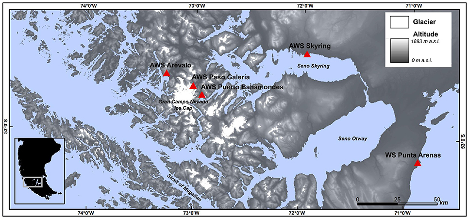
Figure 1. Location of automatic weather stations (AWS) at the Gran Campo Nevado Ice Cap and the weather station (WS) at Punta Arenas. Glacier outlines are based on the Randolph Glacier Inventory 6.0.

Large-scale modes of climate variability like the El Niño Southern Oscillation (ENSO) and Antarctic Oscillation (AAO), also known as the Southern Hemisphere Annular Mode (SAM), significantly influence precipitation and air temperature in southern South America (e.g., Thompson and Solomon, 2002; Marshall, 2003; Schneider and Gies, 2004; Fogt and Bromwich, 2006; Gillett et al., 2006). ENSO influences the interannual climate variations in the subtropical parts of South America, and weakens toward the southern tip of South America (Aceituno, 1988; Schneider and Gies, 2004; Gillett et al., 2006; Aravena and Luckman, 2009; Garreaud et al., 2009). Intensified positive AAO phases lead to a strong temperature and precipitation response (Gillett et al., 2006; Aravena and Luckman, 2009; Garreaud et al., 2009).

Climate variability in Southern Patagonia is the key driver of local changes in the cryosphere (e.g., Möller et al., 2007; Davies and Glasser, 2012). A variety of environmental paleorecords offer the possibility to study climate changes and short term climate variability (e.g., storm events) in Southern Patagonia from the late Holocene to the Last Glacial Maximum and beyond (e.g., Villalba et al., 2003; Lamy et al., 2010; Kilian and Lamy, 2012). However, the network of long-term meteorological observations which is needed to calibrate paleoclimate proxies for example from dendro-climatology (Aravena et al., 2002), sediment (Kilian et al., 2007) or peat cores (Kilian et al., 2003, 2007) as well as recent (Schneider et al., 2007) and Holocene (Koch and Kilian, 2005; Kilian et al., 2013) glacier fluctuations in the Southern Andes is still sparse in Southernmost Patagonia. The mass balance modeling study of Möller and Schneider (2008) indicate a pronounced mass-balance sensitivity of the GCN Ice Cap to temperature. The presented meteorological time series provide the opportunity to study the climate forcing on recent changes of the ice cap. The quality of future surface mass balance modeling studies benefits significantly from such unique long-term time series.

Here, we revise and extend former climate studies at the GCN Ice Cap (Schneider et al., 2003; Schneider and Gies, 2004) by analyzing the main climate features and their variability. Meteorological observations since 2000 provide more robust estimates of the observed annual and seasonal means, anomalies, extremes and trends. The characteristics are related to mesoscale weather patterns, classified by a hierarchical correlation-based leader algorithm. Annual and seasonal trends in air temperature are investigated by applying the non-parametric Mann-Kendall and Sen slope estimator trend test (Mann, 1945; Kendall, 1975; Yue et al., 2002). Furthermore, we focus on how ENSO and AAO impact the regional climate.

2. Data

2.1. Observations

We analyze meteorological time series of four AWS located close to the GCN Ice Cap and one conventional weather station (WS) at Punta Arenas in Chile (Figure 1). An overview of the pertinent data is given in Table 1. Detailed information about the geographical setting of AWS Paso Galería (PG), AWS Puerto Bahamondes (BH) and AWS Estancia Skyring (SR) is given in Schneider et al. (2003). In addition, a fourth AWS named Arévalo (AR) has operated since September 2007 and is located at the northwestern side of the ice cap at about 58 m a.s.l.

TABLE 1

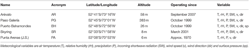
Table 1. Pertinent data to the weather station and automatic weather stations used in this study.

The AWS are manufactured by Campbell Scientific Ltd. (United Kingdom). The similarly designed stations are equipped with sensors of air temperature, air humidity, precipitation, solar radiation, wind speed and wind direction (Table 2, Figure S1). All meteorological variables but precipitation are measured at 2 m above the surface. Precipitation is measured at 1 m above the ground using unshielded tipping-bucket rain gauges. This type of measurement underestimates precipitation by up to 30% at wind speeds of 1.5 m s⁻¹ and even up to 50% at wind speeds of 3.0 m s⁻¹ (Rasmussen et al., 2012; Buisán et al., 2017). Wind-speed induced deviations increase during snowfall due to an intensified drifting of snow (Rasmussen et al., 2012; Buisán et al., 2017). Substantial deviations are further suspected during high precipitation events, since strong precipitation events are often accompanied with strong wind gusts. During periods with very strong winds, the tipping bucket tends to shake which leads to an overestimation of precipitation. Correction factors for this kind of inaccuracy are not available. According to Schneider et al. (2003), the precision of the precipitation measurement at AWS BH and AWS PG is estimated to be about ±20%. We used this number as estimate of uncertainty for all AWS in this study. Wind-speed induced deviations have been minimized due to an additional fixation of the rain gauges in 2010 at AWS PG and in 2016 at AWS BH to avoid the shaking of the tipping bucket. Overall, precipitation data must be interpreted with care bearing in mind that these data are subject to considerable uncertainty in the order of potentially several tens of percent. Meteorological observations at the conventional WS Punta Arenas (PA) hold the longest and most complete time series. These observations (2000-2016) are measured according to the World Meteorological Organization standards. Data are provided by the Laboratory of Climatology, Instituto de la Patagonia, Universidad de Magallanes. Yearly records are published in Anales del Instituto de la Patagonia, Chile (e.g., Butorovic, 2016).

TABLE 2

Table 2. Instrumentation at AWS Paso Galería, AWS Puerto Bahamondes, AWS Arévalo, and AWS Skyring as used in this study.

The quality of the time series is assured by performing some basic quality integrity and outlier checks (Durre et al., 2010). In case of unrealistic values, such as relative humidity larger than 100%, identical values for maximum and minimum air temperature, or a repetition of data records within a month, data are excluded. Furthermore, records are checked for daily outliers (Durre et al., 2010) and missing values within a month. Months with missing values of daily observations are not further considered. In case of precipitation, this leads to an exclusion of daily precipitation observations at AWS BH in 2000/01 and at AWS PG in 2008/09. In addition, failures of power supply or sensors due to harsh weather conditions cause substantial data gaps in addition. Figure 2 shows the available observation periods for each station on a monthly basis as used in this study.

FIGURE 2

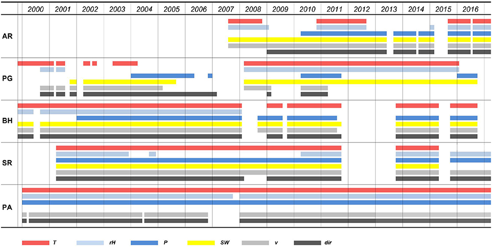
Figure 2. Available observation periods at AWS Arévalo (AR), AWS Paso Galería (PG), AWS Puerto Bahamondes (BH), AWS Skyring (SR), and WS Punta Arenas (PA). Shown are measurement periods of air temperature (T), relative humidity (rH), precipitation (P), incoming shortwave radiation (SW), wind speed (v), and direction (dir).

2.2. Reanalysis Data

For mesoscale weather type classification, daily mean sea level pressure (MSLP) reanalysis data are obtained from the ERA-Interim dataset provided by the European Centre for Medium-Range Weather Forecasts (ECMWF) (Dee et al., 2011). The data sets are downloaded with a spatial resolution of 0.75° × 0.75° grids and 12-hourly temporal resolution (0 a.m., 12 p.m. UTC) between 1979 and 2016 for the area 10°S −80°S and 40°W −110°W covering most of South America and the Antarctic Peninsula. The selected area as well as the choice of MSLP as weather classification variable followed the weather type classification as used by Frank (2002) and Schneider et al. (2003).

2.3. Indices of Large-Scale Modes of Climate Variability

To reveal the impact of ENSO and the AAO on climate variability in Southernmost Patagonia, we compare the monthly anomalies of observations with the Oceanic Niño Index (ONI) and the Antarctic Oscillation Index (AAOI). Both indices are provided by the U.S. National Oceanic and Atmospheric Administration (NOAA) - Climate Prediction Center.

ONI identifies El Niño and La Niña events in the tropical Pacific by using a 3-month running mean of ERSST.v5 sea surface temperature anomalies in the Niño 3.4 region (5°N-5°S, 120°-170°W) (Barnston et al., 1997; Huang et al., 2017). Events are defined as five consecutive overlapping 3-month periods with anomalies ≥+0.5°C for El Niño and ≤ -0.5°C for La Niña events. Data is available from http://www.cpc.ncep.noaa.gov/data/indices/oni.ascii.txt.

The monthly AAOI is constructed by projecting the monthly mean 700 hPa height anomalies poleward of 20°S onto the first empirical orthogonal function mode of monthly mean height anomalies at 700 hPa (Thompson and Solomon, 2002). Positive phases are characterized by a strengthening and poleward shift of the westerlies with decreased surface pressure and geopotential height over the fringe of Antarctica. During negative phases, opposite conditions prevail. Monthly data of AAOI can be obtained from http://www.cpc.ncep.noaa.gov/products/precip/CWlink/daily_ao_index/aao/aao_index.html.

3. Methods

3.1. Indices of Climate Extremes

Climate extremes of air temperature and precipitation (Table 3) are described using selected indices of extremes (Tank et al., 2009). In case of air temperatures extremes, time series of maximum (TX) and minimum (TN) air temperature are analyzed regarding the number of days with ice (TX ≤ 0°C) (ID) and frost (TN ≤ 0°C) (FD). Percentiles are calculated based on the available observations period (Figure 2) to define the number of days with TX < 10th percentile (P1TX), TN < 10th percentile (P1TN), TX > 90th percentile (P9TX) and TN > 90th percentile (P9TN). Furthermore, we are interested in the maximum length of a cold spell (CS) with consecutive days of TN < 10th percentile, and the maximum length of a warm spell (TWS) with consecutive days of TX > 90th percentile per year.

TABLE 3

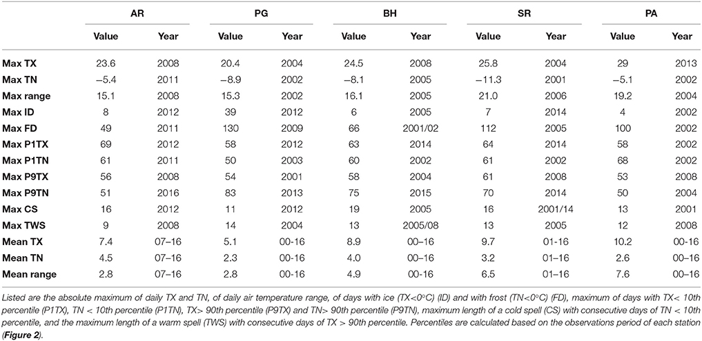
Table 3. Indices of air temperature extremes based on daily maximum (TX) and minimum (TN) air temperatures.

Precipitation extremes are described by the absolute maximum of 1-Day (PDX) and 5-Day (P5DX) precipitation (mm) as well as the annual amount of daily precipitation larger than the 95th percentile (P95P) and the 99th percentile (P99P). The maximum number of days with daily precipitation higher than 20 mm (HP) and below 1 mm (DD), and the maximum length of wet spells (PWS) and dry spells (DS) per year are also examined.

3.2. Weather Type Classification

Weather types are classified by applying the automated classification map-pattern scheme by Lund (1963) based on MSLP. The LUND-algorithm is based on so-called leader patterns. It constitutes a low computational cost predecessor of other cluster algorithms (Hartigan, 1975; Murtagh, 1985). Within the LUND-algorithm, in a first run a leader is defined as the one observation showing most similar cases (observations) of correlations higher than a given threshold with all other observations (Lund, 1963; Philipp et al., 2014a). After removal of the leader and its matching cases, e.g., all observations that correlate with the identified leader above the set threshold Pearson correlation coefficient, the remaining class leaders are called in similar iterative processes (Lund, 1963; Philipp et al., 2014a). After the determination of all leaders, single days are assigned to a specific weather type by returning all observations to the data pool and assigning each one to the nearest leader based on linear correlation (Lund, 1963; Philipp et al., 2014a). The threshold Pearson correlation coefficient for finding leader weather types in this study is set to 0.85. The Lund classification scheme accentuates the dominance of few weather types with westerly air flow. Subsequently, it finds further weather types that occur only rarely but are important and significantly different patterns. In contrast, k-mean leader algorithms tend to locate centroids in such that all classes become equally large (Philipp et al., 2014b). The latter would have resulted in many undesirably similar weather types of principally westerly airflow.

Weather type classifications are calculated from the ERA-Interim MSLP reanalysis data for the period 1979–2016. We apply the cost733class-1.2 software (http://cost733.geo.uni-augsburg.de/cost733class-1.2) originally designed for circulation type classifications in Europe (Philipp et al., 2014b). We checked for the optimal number of classes using a k-means leader algorithm by evaluating the increase of explained cluster variance with increasing numbers of cluster. The number of 10 weather types was found to be optimal which is in accordance with the weather type classification of Frank (2002), used by Schneider et al. (2003). Earlier weather type classifications document only six weather types (Endlicher, 1991; Compagnucci and Salles, 1997). Figure 7 shows the resulting 10 MSLP centroids obtained from the classification procedure after Lund (1963) as used in this study.

3.3. Trend Detection

Annual and seasonal trends in air temperature based on the 17-year record of AWS PG, AWS BH, AWS SR, and WS PA are analyzed. Air temperature changes over the given time period can further be related to observed recent changes of the GCN Ice Cap outlet glaciers.

Trends are detected using the non-parametric Mann-Kendall (MK) and Sen slope estimator (SSE) trend test. The combined MK and SSE test has been frequently used to quantify the significance and magnitude of trends in climatological and hydrological time series (e.g., Hamed, 2008; Gocic and Trajkovic, 2013; Kisi and Ay, 2014; Onyutha et al., 2016). The MK test is a non-parametric test to identify linear and non-linear trends in time series (Mann, 1945; Kendall, 1975). The test does not require normally-distributed input data and has a low sensitivity to abrupt breaks due to inhomogeneous time series. The magnitude of the trend in terms of slope is the robust estimate of the median following the approach by Sen (1968) and Theil (1950).

The elimination of autocorrelation in time series analysis is essential because otherwise autocorrelation increases the chances of detecting a significant trend even in case trends are absent. Therefore, Yue et al. (2002) proposed the Trend-Free Pre-Whitening (TP) method in case both trend and lag-1 autocorrelation exist in the data record.

To detect trends in the time series we followed the described steps below:

• testing the significance of the lag-1 autocorrelation (AC) in each time series (step 1)

• in case of significant AC, TP is applied (step 2) and the MK and SSE tests are applied subsequently

• in case of insignificant AC, the MK and SSE tests are performed directly on the original time series (step 3)

The Trend-Free Pre-Whitening procedure (step 2) includes the following steps. First, the apparent linear trend of the time series X_i is removed. Afterward, the lag-1 correlation coefficient r_ac of the detrended time series X_DE,i is determined. The lag-1 AC is then eliminated from X_DE,i by:

$\begin{array}{ll}{X}_{DE,A,i}=X_{DE,i}-r_{ac}·X_{DE,i-1}.& (1)\end{array}$

The removed linear trend is then added to X_DE,A,i to obtain the final blended time series to which the MK and SSE trend detection test is applied.

4. Results and Discussion

4.1. Time Series and Extremes

Time series of air temperature, relative humidity, precipitation, wind speed and wind direction are analyzed regarding their daily, monthly and annual means, and anomalies. Mean annual and monthly values of the meteorological variables for each station are listed in Table S1 in the supplement. Annual means are averaged based on monthly mean values. The study period of each time series relates to the available observation period shown in Figure 2.

4.1.1. Air Temperature

Mean annual air temperatures for the individual measurement period of each station (Figure 2) along the west-east transect are 5.8°C at AWS AR, 3.8°C at AWS PG, 6.0°C at AWS BH, 6.6°C at AWS SR, and 6.6°C at WS PA.

The air temperature distribution in mountain areas with strong orographic effects can also be detected in the spatial distribution of mean daily maximum and minimum air temperature and air temperature range (Table 3). The absolute extremes of daily air temperatures range from −8.9°C and +20.4°C at AWS PG, from −8.1°C and +24.5°C at AWS BH, and −11.3°C and +25.8°C at AWS SR during the observation period 2000 to 2016.

The coldest temperature regime with the lowest mean of daily maximum temperature of +5.1°C and minimum temperature of 2.3°C is found at AWS PG. The numbers of frost and ice days are larger than at the other stations due to the altitude and contiguity to the ice cap (Table 3). In 2009, minimum temperature dropped below 0°C in 36% of the days. The lower amplitudes of the annual temperature cycle of AWS AR and AWS BH are a result of more maritime conditions compared to AWS SR and WS PA (Figure 3, Table S1). The influence of the Pacific Ocean also leads to less days with frost and ice. Toward the east the mean annual temperatures and the number of days with daily maximum air temperature exceeding the 90th percentile and daily minimum air temperature dropping below the 10th percentile increase.

FIGURE 3

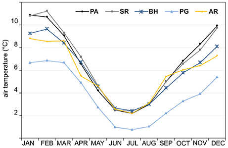
Figure 3. Mean monthly air temperature at AWS Arévalo (AR), AWS Paso Galería (PG), AWS Puerto Bahamondes (BH), AWS Skyring (SR), and WS Punta Arenas (PA) averaged over the individual observation period (Figure 2).

Figure 4 illustrates the monthly means of air temperature and anomalies since 2000, showing a high correlation of r = 0.94–0.99 in temperature variability between all stations. Above average cold months were observed in spring 2000, winter 2002 and 2005, spring 2009 and summer 2011/12 at all stations. The longest cold spell and the largest numbers of days where the maximum temperature drops below the 10th percentile for AWS AR and AWS PG are found in 2012 (Table 3). Positive anomalies occurred during winter 2003, the summer months 2003/04 and during winter 2016.

FIGURE 4

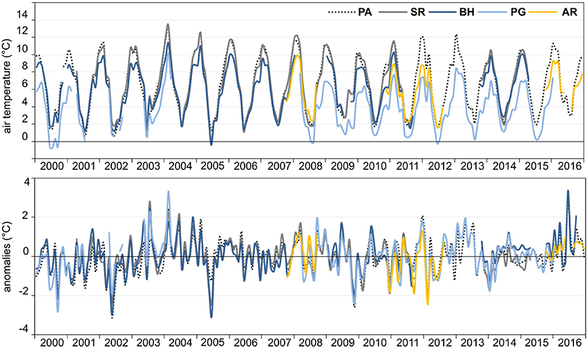
Figure 4. Monthly air temperature and monthly anomalies at AWS Arévalo (AR), AWS Paso Galería (PG), AWS Puerto Bahamondes (BH), AWS Skyring (SR), and WS Punta Arenas (PA) from 2000 to 2016.

The annual anomalies of mean, maximum and minimum temperatures suggest in general milder climate conditions with less extremes since 2012 at GCN (Tables S2, S3). This observation is supported by lower annual means of daily temperature ranges and a decreasing number of days with frost per year at all stations. Furthermore, the percentage of days per year with extreme warm (P9X) or cold conditions (P1N) are decreasing as well (Table S3). Annual changes in the duration of cold or warm spells, however, are not significant. We hypothesize that the warmer conditions are caused by the strengthening of the westerlies during the enhanced positive AAO in recent years (Marshall, 2003).

4.1.2. Wind Speed and Direction

The prevailing westerlies dominate the wind patterns year-around at GCN with mean annual wind speeds ranging from 3.1 m s⁻¹ (AWS BH) to 5.1 m s⁻¹ (AWS PG) (Figure 5). The highest mean of daily mean and maximum wind speeds of 5.1 m s⁻¹ and 13.4 m s⁻¹ are observed at AWS PG along with prevailing north-west winds. Mean wind speeds of 3.1 m s⁻¹ at AWS BH are lower than at AWS SR and WS PA with values of 3.7 m s⁻¹ and 4.5 m s⁻¹, respectively. The mean maximum wind speed of 9.7 m s⁻¹ at AWS BH, however, is higher than at AWS SR (8.0 m s⁻¹). Schneider et al. (2003) pointed out that this underscores the occurrence of strong gusty winds in morphologically structured landscapes. In general, mean and maximum wind speeds decrease during the winter months at all stations but AWS AR. The characteristic southerly winds at AWS AR are caused by the topographic situation channeling the airflow.

FIGURE 5

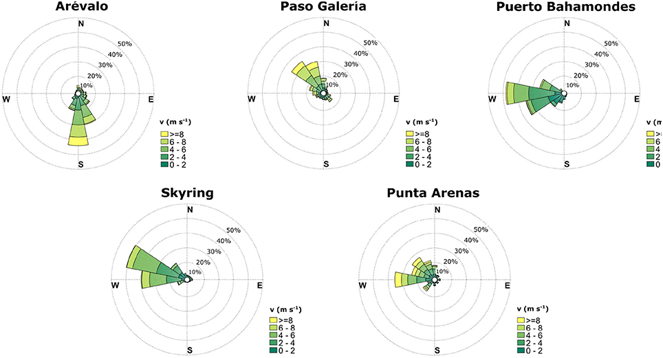
Figure 5. Frequency of wind direction and wind speed (v) at AWS Arévalo, AWS Paso Galería, AWS Puerto Bahamondes, AWS Skyring, and WS Punta Arenas. The available observation period for each station can be found in Figure 2.

4.1.3. Precipitation

A sharp gradient of precipitation can be found across the GCN Ice Cap within only tens of kilometers. Mean annual precipitation (2008–2016) increases from ~3,800 mm at the west side of GCN at AWS AR to ~6,100 mm at AWS PG while it decreases again on the lee-side to ~4,000 mm at AWS BH. Within a distance of about 80 km, precipitation sharply drops to ~790 mm at AWS SR. Mean annual amounts of 570 mm are observed at WS PA for the same study period. Considering the observations at AWS PG since 2002, the annual mean accounts for ~7,500 mm with the highest annual amount of ~9,500 mm measured in 2003. Higher measurement inaccuracies in the first years of precipitation observations must be assumed due to the less firm installation of the rain gauge. Therefore, the estimated mean annual values of AWS PG (10,900 mm ±20%) and AWS BH (6,600 mm ±20%) as provided by Schneider et al. (2003) are resulting from measurement errors during episodes of strong winds, leading to an overestimation of annual precipitation sums between 2000 and 2003.

The intra-annual variability of precipitation at AWS AR, AWS PG, and AWS BH correlates well with the highest amounts occuring during the austral summer. The drop in monthly precipitation in February is revealed at all three stations (Figure 6). The annual course at AWS SR is more similar to the ones at GCN, but with much lower precipitation, while the intra-annual variability at WS PA is opposite. Precipitation during the winter is slightly higher than during the austral summer. Inter-annual variations of precipitation between AWS SR and AWS PA show opposite patterns. In years with positive precipitation anomalies at AWS SR, precipitation mostly decreases at AWS PA (Table S2). In principal, the same holds true for AWS BH and AWS PA for the few full years of available precipitation data.

FIGURE 6

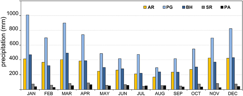
Figure 6. Mean monthly precipitation AWS Arévalo (AR) (2008-2016), AWS Paso Galería (PG), AWS Puerto Bahamondes (BH), AWS Skyring (SR), and WS Punta Arenas (PA). Values were averaged from 2000 to 2016.

The occurrence of high precipitation events of up to 620 mm in 5-days in 2004 and wet spells of up to 61 days in 2006 underscore the year-around wet conditions at GCN (Table 4). Individual events of extreme precipitation (P5DX, P95P, P99P) are most frequent at AWS PG. Between 2002 and 2006, 26% of the annual amount of precipitation fell during days where the daily precipitation exceeds the 95th percentile (Table S4). This ratio changes to a mean of 8% in 2010, 2011, 2016. The amounts of precipitation during extreme precipitation events and days with daily precipitation larger than 20 mm (HP) are similar between the western (AWS AR) and eastern side (AWS BH) of GCN with a high year-to-year variability between 2011 and 2016. The percentage of HP is negligible for AWS SR and WS PA. Nevertheless, daily extreme events of up to 124 mm can occur at AWS SR as observed in 2010. The lengths of wet spells are subsequently smaller while the lengths of dry spells are much larger compared to the three stations at GCN (Table 4).

TABLE 4

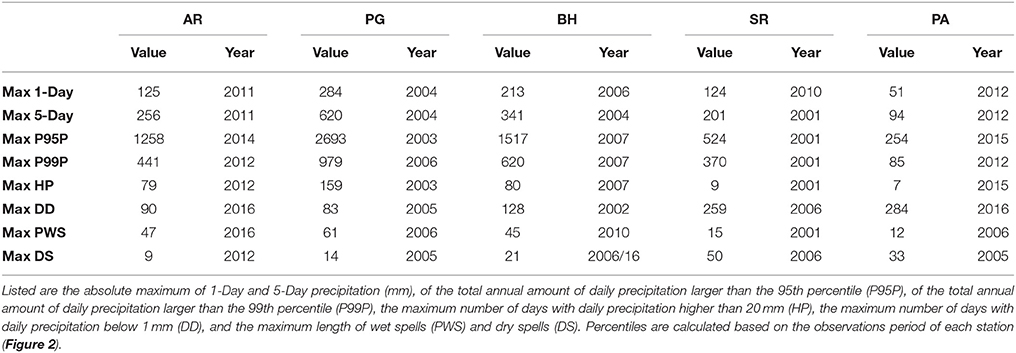
Table 4. Indices of precipitation extremes.

4.2. Trends

Annual and seasonal trends in mean (T), minimum (TN) and maximum (TX) air temperature are analyzed for AWS PG, AWS BH, AWS SR, and WS PA as described in section 3.3. Significant lag-1 autocorrelation was only detected for TN of AWS BH which was corrected following the TP procedure before trend detection. An overview of the trend analysis results is given in Table 5.

TABLE 5

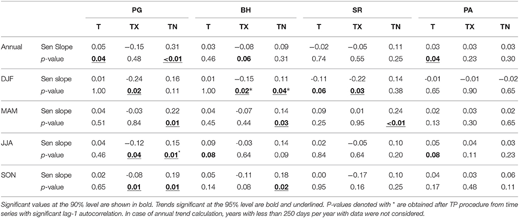
Table 5. Statistical results of the trend analysis for annual and seasonal mean (T), maximum (TX), and minimum (TN) air temperature in °C a⁻¹ for AWS Paso Galería (PG), AWS Puerto Bahamondes (BH), AWS Skyring (SR), and WS Punta Arenas (PA).

Trends in annual mean air temperature for AWS PG and AWS PA are significant at the 90% level with a trend magnitude (Sen Slope) of +0.05°C a⁻¹ and +0.02°C a⁻¹. An increasing trend of seasonal mean air temperature is only apparent during winter (JJA) at AWS BH and WS PA. A significant upward trend is detected in the annual TN at AWS PG of +0.31°C a⁻¹ between 2000 and 2016. This upward trend is also reflected in different seasons as well. TN increases significantly during spring (SON), winter and fall (MAM) at AWS PG, and during summer (DJF), spring and fall at AWS BH. Three of four stations show upwards trends of TN during spring and fall. In contrast, significant downward trends of TX during the summer season are determined for AWS PG, AWS BH and AWS SR. The largest trend of −0.24°C a⁻¹ (2000 and 2016) was found at AWS PG. No significant trend has been detected in annual and seasonal TX time series for WS PA.

4.3. Types of Synoptic Weather Patterns

Ten major types of synoptic weather patterns have been classified for Southernmost Patagonia (Figure 7). Weather type 1 is characterized by a strong north-south pressure gradient resulting from a distinct high-pressure cell over the Pacific and low-pressure trough over the Bellingshausen Sea, which leads to intensified westerlies. During weather type 2, the high-pressure cell is weaker and shifted toward the south, while the low-pressure cell is located south of Tierra del Fuego in the Weddell Sea. Cold and humid air masses from the south-west are advected to Southernmost Patagonia (Frank, 2002). A similar circulation pattern to type 2, but with a distinct low-pressure cell located south of Tierra del Fuego in the Drake Passage occurs during weather type 5. A north-westerly advection of humid and warm air occurs when both, the Pacific anticyclone and the low-pressure cell, are shifted toward the north-west of southern South America compared to type 1. Pressure gradients become weaker during weather type 9 while the principal synoptic configuration is mostly the same.

FIGURE 7

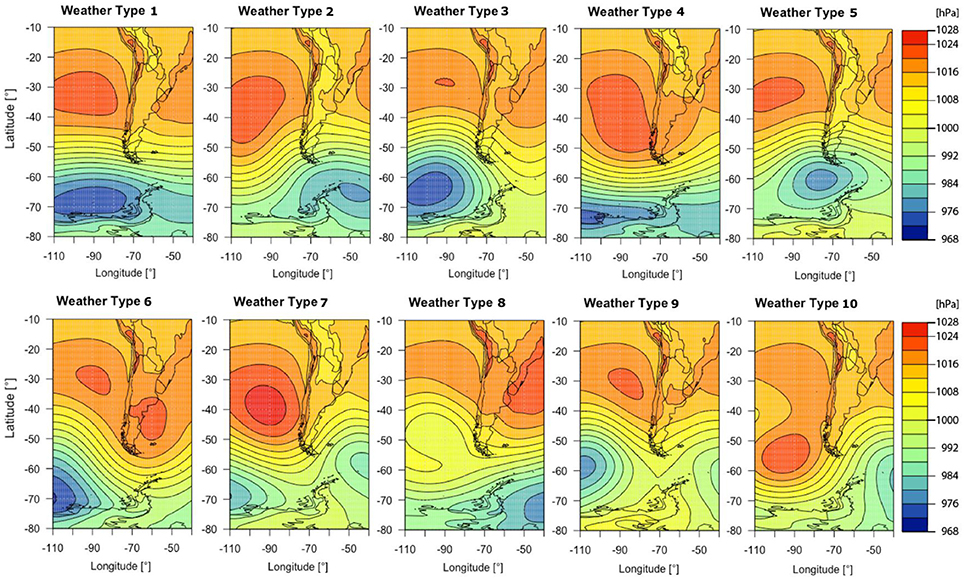
Figure 7. Ten major weather types classified by means of ERA-Interim MSLP reanalysis data for the period 1979 to 2016.

The atmospheric circulation of weather type 4 is dominated by an intensified high-pressure cell in the southern Pacific reaching far toward the eastern side of the Southern Andes. The persistence of this situation leads to warmer and dryer conditions. A southward shift of the Pacific anticyclone with the advection of colder air masses from south-west, is present during weather type 7. A strong high-pressure cell in the southern Atlantic accompanied with low pressure in the southern Pacific is present during weather type 6. The Atlantic anticyclone is stronger and shifted toward the north in case of type 8. Both weather patterns imply a northerly or westerly airflow with increased air temperatures. The circulation pattern of weather type 10 is dominated by a strong high-pressure cell located far toward the south in the Pacific leading to a cold and humid airflow from the south over Southernmost Patagonia.

Major synoptic weather types with distinct low-pressure cells in the Weddell Sea (types 2 and 5) or Bellingshausen Sea (types 1, 3, and 9), causing a prevailing southwesterly, northwesterly or westerly airflow, account for 68% of all days in Southernmost Patagonia. In 32% of all situations, high pressure cells over the southern Pacific (types 4, 7, and 10) and southern Atlantic (types 6 and 8) determine the weather of Southernmost Patagonia. Circulation pattern type 1 with a strong zonal westerly air flow is the most common type of all weather patterns, occurring 30% of the year (Figure 8, Table 6). During the austral summer the frequency of weather patterns with westerly air flow increases to 76% compared to high-pressure influenced weather types (24%). During the austral winter anticyclonic circulation patterns account for 40% of all situations, while low-pressure weather types occur less. This is in accordance with the generally lower wind speeds found in winter at all weather stations in this study.

FIGURE 8

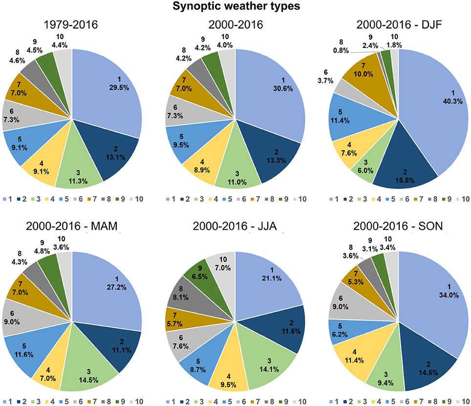
Figure 8. Frequencies of synoptic weather types averaged between 1979 and 2016, 2000 and 2016 and for summer (DJF), fall (MAM), winter (JJA) and spring (SON) between 2000 and 2016.

TABLE 6

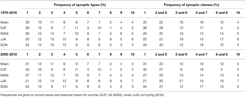
Table 6. Frequency of synoptic weather types and classes (%) between 1979 and 2016 and 2000 and 2016.

Anomalies of observed air temperature, precipitation, wind speed, solar radiation, and relative humidity are analyzed according to the major synoptic types of weather patterns for all five stations (Figure 9). Similar types of weather patterns are grouped into classes as listed in Table 6. Large positive air temperature anomalies are accompanied with strong westerlies (class 1) at all five stations. Air temperature anomalies at AWS BH, AWS AR, and AWS PG however are smaller compared to AWS SR and WS PA due to the influence of the nearby GCN Ice Cap and proximity to the Pacific Ocean. The impact of strong westerlies on air temperature anomalies is largest in the austral fall. On days with southwesterly airflow (class 2 and 5), air temperatures slightly drop at the stations located close to GCN Ice Cap, while air temperatures tend to rise during northwesterly airflow (class 3 and 9). The advection of colder air masses from the southwest (class 2 and 5) largely determines the air temperature variability during the summer and fall season.

FIGURE 9

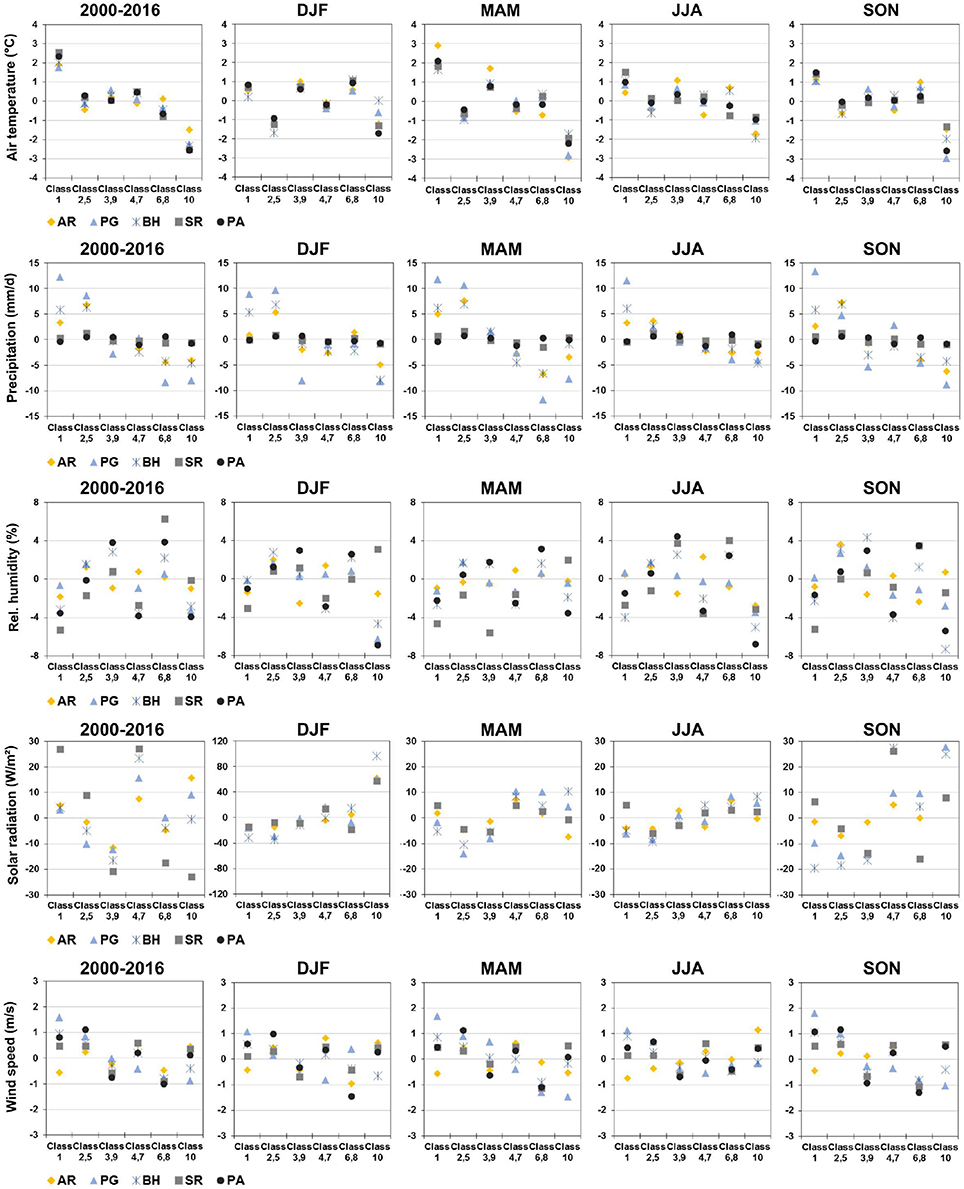
Figure 9. Daily anomalies of air temperature, precipitation, relative humidity, solar radiation, and wind speed for each class of synoptic weather patterns between 2000 and 2016 and for summer (DJF), fall (MAM), winter (JJA), and spring (SON) between 2000 and 2016.

The impact of circulation patterns with intensified high-pressure cells in southern Pacific and Atlantic (classes 4 and 7, 6 and 8 and 10) on air temperature variability is in general low, but highest for AWS SR and WS PA. The advection of air masses from the north and northwest under high-pressure influence (class 6 and 8) cause warmer conditions at all stations in SON and DJF, while temperatures decrease during the austral winter except for AWS AR which is the only station located clearly west of the Cordillera. The advection of cold air masses from the south (class 10) causes a significant decrease of daily air temperature at all stations with the largest negative anomalies for WS PA and AWS SR. During fall and spring, air temperatures drop significantly below the specific means (class 10).

Circulation patterns highly impact the precipitation variability at the GCN Ice Cap during all seasons. The orographic induced uplift of the humid air masses from west and southwest (classes 1 and 2 and 5) comes along with year-around positive precipitation anomalies at the GCN Ice Cap. Precipitation amounts decrease significantly during high-pressure influences, in case of classes 6 and 8 and 10. The stations located at GCN (AWS AR, AWS BH, AWS PG) obtain more than 80% of daily precipitation during westerly airflow. East of the GCN Ice Cap at AWS SR and WS PA, mean daily precipitation amounts are similar during all weather types. Precipitation increases slightly on days with southwesterly air flow at AWS SR, while at WS PA daily precipitation increases on days with north to northwesterly wind directions (classes 3 and 9 and 6 and 8). The annual precipitation amounts at AWS SR and WS PA are still mainly determined by the airflow from west (class 1) and south west (class 2 and 5) despite the fact that these stations are clearly located on the leeward of the Cordillera during westerly air flow but extreme precipitation rates are rare. Of all daily precipitation extremes (higher than the 90th percentile) 80% can be associated with classes 1 and 2 and 5 at the GCN stations, while the percentage decreases to 70% at AWS SR and 51% at WS PA. High precipitation events at WS PA are also present during the class 3 and 8 with 20 and 13% of the days, respectively. This finding indicates that precipitable water in the air column is carried across the Cordillera by strong upper air westerly winds. During classes 1 and 2 and 5, both stations experience often foehn-type weather conditions with cloud dispersal due to the subsidence of air masses on the lee-side of the Cordillera. High incoming solar radiation can therefore be observed at AWS SR during these types of weather patterns. Since the westerly air flow is also accompanied by higher air temperatures, relative humidity decreases at all stations, but strongest at AWS SR and WS PA.

Wind speed is highest during westerly (class 1) and southwesterly (class 2 and 5) airflow for all stations. AWS AR shows negative wind speed anomalies on days with strong westerlies which are caused by the location of the AWS and local effects due to the surrounding topography as described in section 4.1.2. Wind from north-northwest (classes 3 and 9 and 6 and 8) is in general weaker on days with high-pressure influence (class 6 and 8).

4.4. Teleconnection to El Nino-Southern Oscillation and Antarctic Oscillation

4.4.1. Time Series

Most of the monthly anomaly records show significant lag-1 autocorrelations at the 95% level which were eliminated before removing the trend as described in section 3.3. Time series are then correlated to ONI and AAOI also considering time lags of up to +3 months. Correlations between monthly anomalies of mean (T), maximum (TX), and minimum (TN) air temperature, rel. humidity (rH), precipitation (P) and wind speed (v), and monthly ONI and AAOI are listed in Table 7.

TABLE 7

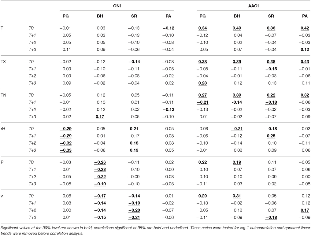
Table 7. Correlation between ONI and AAOI and monthly anomalies of mean (T), maximum (TX), and minimum (TN) air temperature, relative humidity (rH), precipitation (P) and wind speed (v) at AWS Paso Galería (PG), AWS Puerto Bahamondes (BH), AWS Skyring (SR), and WS Punta Arenas (PA) for different time lags (T0 to T+3 months).

Correlations between monthly anomalies and ONI are weak (Table 7, Figure 10), which is consistent with previous studies (Schneider and Gies, 2004; Garreaud et al., 2009). Since 2000 seven cold (ONI ≤-0.5) and five warm (ONI≥ +0.5) periods have been observed. A significant negative correlation of −0.26 can be identified for precipitation anomalies at AWS BH. Monthly precipitation decreases by −9% (−32 mm) during El Niño events (ONI≥ +0.5) at AWS BH compared to the monthly mean (2000-2016) while it increases by +9% during La Nina events (ONI ≤ −0.5) (Table 8). The influence of ENSO on precipitation variability diminishes further to the east of the Southernmost Andes (Table 7). These findings are similar to Schneider and Gies (2004). However, only for AWS BH there is an indication that ENSO events may influence precipitation at GCN in the way as it is argued by Schneider and Gies (2004). Significant correlations between precipitation and ONI for any other AWS at GCN are not evident.

FIGURE 10

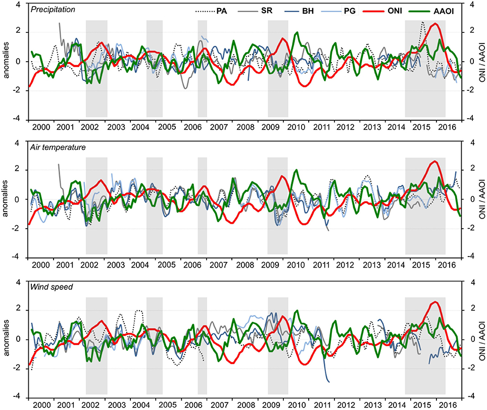
Figure 10. Standardized monthly anomalies of precipitation, mean air temperature and wind speed at AWS Paso Galería (PG), AWS Puerto Bahamondes (BH), AWS Skyring (SR), and WS Punta Arenas (PA) and monthly ONI and AAOI values. El Niño events based on a threshold of +0.5°C for ONI are highlighted by the gray shading. Standardized monthly anomalies of climate variables are illustrated as a 3-month running mean.

TABLE 8

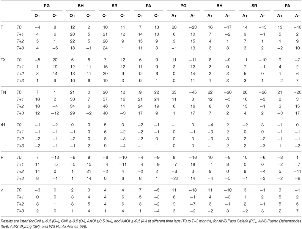
Table 8. Deviations (%) of monthly mean (T), maximum (TX), and minimum (TN) air temperature, relative humidity (rH), precipitation (P) and wind speed (v) from the monthly means (2000-2016) during positive and negative ENSO and AAO phases.

The link between AAO and the climate conditions at GCN and Punta Arenas is evident (Table 7, Figure 10). Positive correlations are significant for T, TX, TN at time-lag T0 for all four stations. Correlations range from +0.34 to +0.49 for T, +0.38 to +0.43 for TX and +0.22 to +0.39 for TN. Highest correlation values are found at AWS BH and WS PA. Anomalies of relative humidity (r = −0.21), wind speed (r = +0.31) and precipitation (r = +0.19) of AWS BH are also linked to AAO.

It is known that positive phases of AAO are associated with dryer and warmer conditions in southern South America (Gillett et al., 2006) which becomes evident in this study as well. The strengthening of the westerlies during positive AAO phases come along with an increase of mean monthly air temperatures by +20% (+0.6°C) at AWS PG, +16% (+1.1°C) at AWS BH, +14% (+1.0°C) at AWS SR and 13% (+0.9°C) at WS PA compared to the monthly average (2000-2016) (Table 8). Colder conditions with up to 23% (−1.0°C) below the average (AWS PG) occur during negative phases of AAO in Southernmost Patagonia. Deviations of TN between the monthly mean during negative and positive AAO phases compared to the overall mean varies between −45% (−1.2°C) to +33% (+0.6°C) at AWS PG, −26% (−1.0°C) to +22% (+0.9°C) at AWS BH, -26% (−0.8°C) to +26% (+0.8°C) at AWS SR, and −20% (−0.6°C) to +21% (+0.6°C) at WS PA. Air temperature increase during positive AAO phases is accompanied by positive precipitation and wind speed anomalies at the GCN stations. Deviations in monthly precipitation between negative and positive AAOI and the overall mean range from −16% (−96 mm) to 8% (+48 mm) at AWS PG, −9% (−32 mm) to +10% (+34 mm) at AWS BH and −6% (−4 mm) to +10% (+7 mm) at AWS SR (Table 8).

4.4.2. Types of Synoptic Weather Patterns

We further analyze how the frequency of the major types of synoptic weather patterns changes during positive and negative phases of AAO and ENSO between 2000 and 2016 (Table 9). The impact of AAO on the synoptic situation in Southernmost Patagonia is largest for the synoptic classes 1, 2 and 5 and 10 since the AAO implies a weakening or strengthening of the westerly air flow. In case of negative AAO phases, days with strong westerly airflow (class 1) decrease by about one third compared to the average, while southwesterly air flow (class 2 and 5) increases by about 41% compared to average (2000–2016). On contrary, during positive AAO phases the westerly airflow dominates the climate at GCN. The high-pressure influence accompanied by cold winds from the south (class 10) is intensified during negative AAO and weakened during positive AAO. This is in good agreement with the observation of air temperature increase in Southernmost Patagonia during positive AAO phases.

TABLE 9

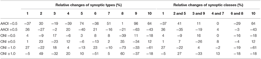
Table 9. Relative changes (%) of synoptic types and classes during positive and negative AAO and ENSO events between 2000 and 2016.

During La Niña events, north-westerly advection of humid air masses (class 3 and 9) is more frequent, while the frequency for circulation patterns with high-pressure influence decreases (classes 6 and 8 and 10). During El Niño events, the frequency of north-westerly airflow decreases while weather classes with high-pressure influence are more present (classes 4 and 7 and 10). Strong La Niña events (ONI≤ −1.0°C) can be associated with enhanced westerlies (+27%) (Table 9), which is consistent with higher precipitation sums at AWS BH (Schneider and Gies, 2004). An intensified low-pressure cell over the Weddell Sea causing southwesterly air flow (class 2 and 5) is enhanced during stronger El Niño events (ONI≥ +1.0°C), while northwesterly airflow (class 3 and 9) occurs less frequently. The frequencies of high-pressure weather classes (classes 6 and 8 and 10) are below the average during both strong El Niño and La Niña events. The impact of ENSO on the variability of synoptic weather patterns generally is rather weak as already identified with respect to the meteorological observations other than precipitation at AWS BH.

5. Conclusion

We analyzed the main features of climate and climate variability in Southernmost Patagonia using a unique 17-year meteorological record (2000–2016) of four AWS in the vicinity of the GCN Ice Cap (53°S). Special attention was given to the link between observed mean, extremes and trends of the AWS records as well as the impact of synoptic weather types and leading modes of global atmospheric variability (ENSO and AAO).

Annual and seasonal trends in air temperature were investigated by applying the non-parametric Mann-Kendall and Sen slope estimator trend test. A weather type classification based on the hierarchical correlations-based leader LUND-algorithm was computed using a 37-year record of ERA Interim Reanalysis data. Major synoptic weather types with distinct low-pressure cells in the Weddell Sea or Bellingshausen Sea causing a prevailing southwesterly, northwesterly or westerly airflow, determine the weather conditions in Southernmost Patagonia during 68% of the time. Circulation patterns with high-pressure cells over the Southern Pacific and Atlantic are present on 32% of all days between 2000 and 2016. The predominance of weather types with humid westerly airflow leads to significant west-east gradients of precipitation and relative humidity across the GCN Ice Cap. Mean annual precipitation (2008 to 2016) increases from ~3,800 mm at the west side of GCN at AWS AR to ~6,100 mm at AWS PG while it decreases again on the lee-side to ~4,000 mm at AWS BH. Within a distance of tens of kilometers precipitation sharply drops to below 800 mm further to the east. More than 80% of extreme precipitation events (>90th percentile) at GCN appears during synoptic types with strong westerly air flow. The occurrence of high precipitation events of up to 620 mm in 5 days and wet spells of up to 61 consecutive days underscore the year-around wet conditions at GCN. High precipitation events and long wet spells become less frequent toward the east of GCN.

We further identify extremes of daily maximum and minimum air temperatures of up to +25.8°C and -11.3°C along with the largest daily temperature range being located on the east side of GCN. Days with daily maximum temperatures exceeding the 90th percentile and days with daily minimum temperature falling below 0°C are less frequent since 2012 indicating a stronger maritime influence in the study region in recent years which might be attributable to increased positive AAO in recent years (Marshall, 2003). Mean annual air temperature increases by +0.05°C a⁻¹ at GCN and +0.02°C a⁻¹ at AWS Punta Arenas during the study period (2000–2016).

The influence of ENSO on intra-annual precipitation and temperature variations is not evident for all investigated stations. At AWS BH precipitation decreases by -9% compared to the monthly mean (2000-2016) during El Niño events while it increases by +9% during La Niña events. The evolution of the AAO determines the synoptic weather types along with air temperature and precipitation variations. Positive AAO phases on average are linked to an intensified westerly airflow (type 1) and warmer conditions in Southernmost Patagonia. Circulation patterns with high-pressure influence leading to colder and dryer conditions in Southernmost Patagonia are more frequent during negative AAO phases.

Author Contributions

SW processed and analyzed the data and drafted the manuscript. DS prepared the synoptic weather type classification. TS, RK, CS designed, installed and maintain the measurement network at GCN. All authors discussed the results and jointly worked on the manuscript.

Funding

This study was funded by the CONYCET-BMBF project GABY-VASA, grant No. 01DN15007, by the German Research Foundation project Gran Campo Nevado, grant No. SCHN 680/1-1 and by the German Research Foundation project MANAU, grant No. SA 2339/3-1.

Conflict of Interest Statement

The authors declare that the research was conducted in the absence of any commercial or financial relationships that could be construed as a potential conflict of interest.

Acknowledgments

We thank Marcelo Arévalo, Marco Möller, Paul Bumeder, Michael Glaser, Johannes Koch, Michael Moritz, Markus Stickling and many others for their help in the field at Gran Campo Nevado Ice Cap during the past 17 years. We are grateful for technical support and advice regarding the weather type classification by Andreas Philipp, University of Augsburg. We thank all reviewers and the editor for their input which helped improving the manuscript considerably.

Supplementary Material

The Supplementary Material for this article can be found online at: https://www.frontiersin.org/articles/10.3389/feart.2018.00053/full#supplementary-material

References

Aceituno, P. (1988). On the functioning of the southern oscillation in the south american sector. part I: surface climate. Monthly Weather Rev. 116, 505–524.

Google Scholar

Aravena, J., Lara, A., Wolodarsky-Franke, A., Villalba, R., and Cuq, E. (2002). Tree-ring growth patterns and temperature reconstruction from nothofagus pumilio (fagaceae) forests at the upper tree line of southern chilean patagonia. Rev. Chil. Hist. Nat. 75, 361–376. doi: 10.4067/S0716-078X2002000200008

CrossRef Full Text | Google Scholar

Aravena, J.-C., and Luckman, B. H. (2009). Spatio-temporal rainfall patterns in southern south america. Int. J. Climatol. 29, 2106–2120. doi: 10.1002/joc.1761

CrossRef Full Text | Google Scholar

Barnston, A., Chelliah, M., and Goldenberg, S. (1997). Documentation of a highly enso-related sst region in the equatorial pacific. Atmosphere-Ocean 35, 367–383. doi: 10.1080/07055900.1997.9649597

CrossRef Full Text | Google Scholar

Buisán, S., Earle, M., Collado, J., Kochendorfer, J., Alastrué, J., Wolff, M., et al. (2017). Assessment of snowfall accumulation underestimation by tipping bucket gauges in the spanish operational network. Atmos. Meas. Tech. 10:1079. doi: 10.5194/amt-10-1079-2017

CrossRef Full Text | Google Scholar

Butorovic, N. (2016). Resumen meteorológico año 2015. estación jorge schythe. Anal. Inst. Patag. 44, 102–110. doi: 10.4067/S0718-686X2016000100009

CrossRef Full Text | Google Scholar

Carrasco, J., Casassa, G., and Rivera, A. (2002). “Meteorological and climatological aspect of the southern patagonia icefield,” in The Patagonia Icefields, eds G. Casassa, F. Sepulveda, and R. Sinclair (New York, NY: Kluwer-Plenum), 29–41.

Google Scholar

Compagnucci, R. H., and Salles, M. A. (1997). Surface pressure patterns during the year over southern south america. Int. J. Climatol. 17, 635–653.

Google Scholar

Davies, B., and Glasser, N. (2012). Accelerating shrinkage of patagonian glaciers from the little ice age (ad 1870) to 2011. J. Glaciol. 58, 1063–1084. doi: 10.3189/2012JoG12J026

CrossRef Full Text | Google Scholar

Dee, D., Uppala, S., Simmons, A., Berrisford, P., Poli, P., Kobayashi, S., et al. (2011). The era-interim reanalysis: configuration and performance of the data assimilation system. Q. J. R. Meteorol. Soc. 137, 553–597. doi: 10.1002/qj.828

CrossRef Full Text | Google Scholar

Durre, I., Menne, M. J., Gleason, B. E., Houston, T. G., and Vose, R. S. (2010). Comprehensive automated quality assurance of daily surface observations. J. Appli. Meteorol. Climatol. 49, 1615–1633. doi: 10.1175/2010JAMC2375.1

CrossRef Full Text | Google Scholar

Endlicher, W. (1991). Zur klimageographie und klimaökologie von südpatagonien. 100 jahre klimatologische messungen in punta arenas. Freiburger Geographische Hefte 32, 181–211.

Fogt, R. L., and Bromwich, D. H. (2006). Decadal variability of the enso teleconnection to the high-latitude south pacific governed by coupling with the southern annular mode. J. Clim. 19, 979–997. doi: 10.1175/JCLI3671.1

CrossRef Full Text | Google Scholar

Frank, A. (2002). Semi-objektive klassifikation und statistische auswertung von wetterlagen südpatagoniens [semi-Objective Classification and Statistical Analysis of Weather Types of South Patagonia]. Master thesis, Univ. Freiburg, Germany.

Garreaud, R., Lopez, P., Minvielle, M., and Rojas, M. (2013). Large-scale control on the patagonian climate. J. Clim. 26, 215–230. doi: 10.1175/JCLI-D-12-00001.1

CrossRef Full Text | Google Scholar

Garreaud, R. D., Vuille, M., Compagnucci, R., and Marengo, J. (2009). Present-day south american climate. Palaeogeogr. Palaeoclimatol. Palaeoecol. 281, 180–195. doi: 10.1016/j.palaeo.2007.10.032

CrossRef Full Text | Google Scholar

Gillett, N. P., Kell, T. D., and Jones, P. D. (2006). Regional climate impacts of the southern annular mode. Geophys. Res. Lett 33:L23704. doi: 10.1029/2006GL027721

CrossRef Full Text | Google Scholar

Gocic, M., and Trajkovic, S. (2013). Analysis of changes in meteorological variables using mann-kendall and sen's slope estimator statistical tests in serbia. Global Planet. Change 100(Suppl. C), 172–182. doi: 10.1016/j.gloplacha.2012.10.014

CrossRef Full Text | Google Scholar

Hamed, K. H. (2008). Trend detection in hydrologic data: the mann–kendall trend test under the scaling hypothesis. J. Hydrol. 349, 350–363. doi: 10.1016/j.jhydrol.2007.11.009

CrossRef Full Text | Google Scholar

Hartigan, J. (1975). Clustering Algorithms. Wiley Series in Probability and Mathematical Statistics. New York, NY: John Wiley & Sons.

Google Scholar

Huang, B., Thorne, P. W., Banzon, V. F., Boyer, T., Chepurin, G., Lawrimore, J. H., et al. (2017). Extended reconstructed sea surface temperature, version 5 (ersstv5): Upgrades, validations, and intercomparisons. J. Clim. 30, 8179–8205. doi: 10.1175/JCLI-D-16-0836.1

CrossRef Full Text | Google Scholar

Kendall, M. (1975). Rank Correlation Methods. London: Griffin.

Google Scholar

Kilian, R., Baeza, O., Breuer, S., Ríos, F., Arz, H., Lamy, L., et al. (2013). Late glacial and holocene paleogeopgraphical and paleoecological evolution of the seno skyring and otway fjord systems in the magellanes region. Anal. Inst. Patag. 41, 7–21. doi: 10.4067/S0718-686X2013000200001

CrossRef Full Text | Google Scholar

Kilian, R., Hohner, H., Biester, H., Wallrabe-Adams, C., and Stern, C. (2003). Holocene peat and lake sediment tephra record from the southernmost andes (53-55°s). Rev. Geol. Chile 30. 47–64. doi: 10.4067/S0716-02082003000100002

CrossRef Full Text | Google Scholar

Kilian, R., and Lamy, F. (2012). A review of glacial and holocene paleoclimate records from southernmost patagonia (49–55°s). Q. Sci. Rev. 53, 1–23. doi: 10.1016/j.quascirev.2012.07.017

CrossRef Full Text

Kilian, R., Schneider, C., Koch, J., Fesq-Martin, M., Biester, H., Casassa, C., et al. (2007). Palaeoecological constraints on late glacial and holocene ice retreat in the southern andes (53°s). Global Planet. Change 59, 49–66. doi: 10.1016/j.gloplacha.2006.11.034

CrossRef Full Text | Google Scholar

Kisi, O., and Ay, M. (2014). Comparison of mann–kendall and innovative trend method for water quality parameters of the kizilirmak river, turkey. J. Hydrol. 513(Suppl. C), 362–375. doi: 10.1016/j.jhydrol.2014.03.005

CrossRef Full Text | Google Scholar

Koch, J., and Kilian, R. (2005). ‘little ice age’ glacier fluctuations, gran campo nevado, southernmost chile. Holocene 15, 20–28. doi: 10.1191/0959683605hl780rp

CrossRef Full Text | Google Scholar

Lamy, F., Kilian, R., Arz, H., Francois, J.-P., Kaiser, J., Prange, M., et al. (2010). Holocene changes in the position and intensity of the southern westerly wind belt. Nat. Geosci. 3, 695–699. doi: 10.1038/ngeo959

CrossRef Full Text | Google Scholar

Lund, I. (1963). Map-pattern classification by statistical methods. J. Appl. Meteorol. 2, 56–65.

Google Scholar

Mann, H. (1945). Nonparametric tests against trend. Econometrica 13, 245–259. doi: 10.2307/1907187

CrossRef Full Text | Google Scholar

Marshall, G. J. (2003). Trends in the southern annular mode from observations and reanalyses. J. Clim. 16, 4134–4143. doi: 10.1175/1520-0442(2003)016<4134:TITSAM>2.0.CO;2

CrossRef Full Text | Google Scholar

Möller, M., and Schneider, C. (2008). Climate sensitivity and mass-balance evolution of gran campo nevado ice cap, southwest patagonia. Ann. Glaciol. 48, 32–42. doi: 10.3189/172756408784700626

CrossRef Full Text | Google Scholar

Möller, M., Schneider, C., and Kilian, R. (2007). Glacier change and climate forcing in recent decades at gran campo nevado, southernmost patagonia. Ann. Glaciol. 46, 136–144. doi: 10.3189/172756407782871530

CrossRef Full Text | Google Scholar

Murtagh, F. (1985). “Multidimensional clustering algorithms,” in COMPSTAT Lectures 4, eds J. M. Chambers, J. Gordesch, A. Klas, L. Lebart, and P. P. Sint (Wien-Würzburg: Physica Verlag), 1–131.

Google Scholar

Onyutha, C., Tabari, H., Taye, M. T., Nyandwaro, G. N., and Willems, P. (2016). Analyses of rainfall trends in the nile river basin. J. Hydroenviron. Res. 13(Suppl. C), 36–51. doi: 10.1016/j.jher.2015.09.002

CrossRef Full Text | Google Scholar

Paruelo, J., Beltran, A., Jobbagy, E., Sala, O., and Golluscio, R. (1998). The climate of patagonia: general patterns and controls on biotic processes. Ecol. Aust. 8, 85–101.

Google Scholar

Philipp, A., Beck, C., Esteban, P., Kreienkamp, F., Krennert, T., Lochbihler, K., et al. (2014a). cost733class-1.2 - User Guide. Available online at: http://cost733.geo.uni-augsburg.de/cost733class-1.2.

Philipp, A., Beck, C., Huth, R., and Jacobeit, J. (2014b). Development and comparison of circulation type classifications using the cost 733 dataset and software. Int. J. Climatol. 36, 2673–2691. doi: 10.1002/joc.3920

CrossRef Full Text | Google Scholar

Rasmussen, R., Baker, B., Kochendorfer, J., Meyers, T., Landolt, S., Fischer, A. P., et al. (2012). How well are we measuring snow: the noaa/faa/ncar winter precipitation test bed. Bull. Am. Meteorol. Soc. 93, 811–829. doi: 10.1175/BAMS-D-11-00052.1

CrossRef Full Text | Google Scholar

Schneider, C., and Gies, D. (2004). Effects of el niño–southern oscillation on southernmost south america precipitation at 53°s revealed from ncep–ncar reanalyses and weather station data. Int. J. Climatol. 24, 1057–1076. doi: 10.1002/joc.1057

CrossRef Full Text | Google Scholar

Schneider, C., Glaser, M., Kilian, R., Santana, A., Butorovic, N., and Casassa, G. (2003). Weather observations across the southern andes at 53°s. Phys. Geogr. 24, 97–119. doi: 10.2747/0272-3646.24.2.97

CrossRef Full Text | Google Scholar

Schneider, C., Schnirch, M., Acuña, C., Casassa, G., and Kilian, R. (2007). Glacier inventory of the gran campo nevado ice cap in the southern andes and glacier changes observed during recent decades. Glob. Plan. Change 59, 87–100. doi: 10.1016/j.gloplacha.2006.11.023

CrossRef Full Text | Google Scholar

Sen, P. (1968). Estimates of the regression coefficient based on kendall's tau. J. Am. Stat. Assoc. 63, 1379–1389.

Google Scholar

Tank, A. K., Zwiers, F., and Zhang, X. (2009). Guidelines on analysis of extremes in a changing climate in support of informed decisions for adaption. Clim. Data Monit. 72, 1–55.

Google Scholar

Theil, H. (1950). A rank-invariant method of linear and polynomial regression analysis. Proc. K. Ned. Akad. Wet., A53, 386–392.

Google Scholar

Thompson, D. W. J., and Solomon, S. (2002). Interpretation of recent southern hemisphere climate change. Science 296, 895–899. doi: 10.1126/science.1069270

PubMed Abstract | CrossRef Full Text | Google Scholar

Villalba, R., Lara, A., Boninsegna, J. A., Masiokas, M., Delgado, S., Aravena, J. C., et al. (2003). “Large-scale temperature changes across the southern andes: 20th-century variations in the context of the past 400 years,” in Climate Variability and Change in High Elevation Regions: Past, Present & Future, ed H. F. Diaz (Dordrecht: Springer), 177–232.

Google Scholar

Weidemann, S., Sauter, T., Schneider, L., and Schneider, C. (2013). Impact of two conceptual precipitation downscaling schemes on mass-balance modeling of gran campo nevado ice cap, patagonia. J. Glaciol. 59, 1106–1116. doi: 10.3189/2013JoG13J046

CrossRef Full Text | Google Scholar

Yue, S., Pilon, P., Phinney, B., and Cavadias, G. (2002). The influence of autocorrelation on the ability to detect trend in hydrological series. Hydrol. Process. 16, 245–259. doi: 10.1002/hyp.1095

CrossRef Full Text | Google Scholar