A Snowpack Forecasting Model for the Eastern Sierra Nevada Based on Cointegration With the North Pacific High Sea-Level Pressure Anomaly

Introduction

Precipitation in the Sierra Nevada mountain ranges of California occurs primarily in the winter months, in the form of snow and rain (Pandey et al., 1999). Meltwaters from accumulated snow, modulated by surface water reservoirs, serve as a source of water supply over the summer months. Snow accumulation over the winter months is carefully tracked to provide an estimate of future snowmelt volumes in the spring and summer months. Typically, reservoirs are operated to maintain sufficient flood storage capacity for the anticipated snowmelt and rain events later in the wet season. Excess runoff is released to maintain flood storage capacity. Advance knowledge of total precipitation during a wet season can allow adjustments in the flood storage capacity to maximize the water stored in the reservoirs.

Here we develop a model, to be used in early February of each year, for forecasting the snow water content (SWC) 2 months later, on April 1, at key Eastern Sierra snow stations on Owens Valley tributary watersheds. Freshwater from this watershed, transported more than 300 miles via aqueducts, is one of the most important water sources for over 4 million people in the Los Angeles metropolitan area (Costa-Cabral et al., 2012). Runoff is managed through reservoirs to support Los Angeles' water supply as well as in-valley uses.

The impetus for this work was the finding by Costa-Cabral et al. (2016) that seasonal precipitation totals in California and other parts of the southwestern United States have a considerably strong relationship with the high-pressure center off the coast of California known as the North Pacific High (NPH). Large-scale climatic indices have been used as predictors of precipitation totals and extremes in many studies and are used operationally in weather forecasts to circumvent the difficulty in obtaining robust dynamical simulations of precipitation.

Establishing a statistical association between observed large-scale climate patterns and precipitation to come in the months ahead is an approach that has been used at many world locations for forecasting precipitation and anticipating water resources availability (for example, Fernando et al., 2015). Such statistical associations have also been used extensively to obtain forecasts of future precipitation based on simulated forecasts of the large-scale climate patterns. Future projections of precipitation have also been obtained on the basis of such statistical associations with large-scale climate patterns (for example, Kharin et al., 2013; Costa-Cabral et al., 2016).

The El Niño-Southern Oscillation (ENSO) phenomenon has been identified as a major driver of climate variability worldwide, and arises from the coupled ocean-atmosphere system of the Pacific basin. Several studies have examined the influence of ENSO on precipitation and temperature over North America, and have documented associations between the strength and phase of ENSO and precipitation frequency and intensity over different regions—particularly the southwestern United States—due to ENSO's influence on the East Asian jet stream position. Thus, California has an increased likelihood of storms, precipitation extremes, and precipitation totals under El Niño conditions (see for example, Chikamoto et al., 2015).

Roughly half the time, however, ENSO is in a neutral phase. Such neutral conditions are not an indication of average meteorology over California. The recent multi-year drought in California provides an example of an extreme meteorological drought occurring at a time when both ENSO and the Pacific decadal oscillation (PDO; Mantua et al., 1997; Zhang et al., 1997) are in near-neutral states. In part due to the oft-neutral state of ENSO, the association of ENSO indices (including the atmospheric-pressure-based SOI index and sea surface temperature-based ENSO3.4 and other indices) with precipitation totals in California is near or below statistical significance level, as is also the case for the PDO as shown e.g., in Costa-Cabral et al. (2016). Rather than ENSO indices, it is the sea level pressure anomaly at the NPH that better reflects the local influence of ENSO, as well as additional variability specific to the North Pacific region.

The strength and position of the NPH, expressed as sea level pressure anomalies and geopotential height anomalies over the northeast Pacific region, affect the position of the jet stream and associated storm tracks. As shown in Costa-Cabral et al. (2016), the positive mode of the NPH is associated with a strong high-anomaly sea level pressure region over the northeastern Pacific. Abnormal northeastern Pacific high pressure ridges that extend from lower- to upper-atmospheric levels can prevent storm systems from reaching California. The role of such high-pressure ridges was discussed during the recent multiyear drought in California, which exhibited the strongest and longer lasting ridge ever observed (e.g., Swain et al., 2014; Wang et al., 2014, 2015; Stevenson et al., 2015). Costa-Cabral et al. (2016) showed that these exceptional high pressure conditions associated with the recent drought fit into a broader pattern documented in reanalysis data.

Costa-Cabral et al. (2016) demonstrated that winter precipitation totals over much of the Southwestern United States hold a special relationship, known as a “cointegration,” with the sea level pressure at the normal location of the NPH. A cointegrated relationship between two stochastic variables exists when, although they appear to vary independently, the cumulative departure from the mean of the two variables tends to remain within a limited distance (Engle and Granger, 1987).

By exploiting the cointegrated relationship between SWC and the NPH anomaly, two models were developed to estimate seasonal precipitation for the Owens River watershed, and provide advance information to support reservoir operations in the Owens Valley:

• The VECM Model Vector Error Correcting Model (VECM) is designed to forecast, in early February, the April 1 SWC value. The VECM model uses the observed annual time series of three variables: (a) the observed January mean of the NPH anomaly, (b) the observed February 1 SWC, and (c) the April 1 SWC at each location of interest. The VECM model exploits the cointegrated relationship between these three variables, and provides a forecast for April 1 SWC based on a linear function of the values of the cumulative sum over time of standardized anomalies of all three variables.

• The Categorical Model is designed to determine the probability, in early February, of the April 1 SWC value falling into the dry, normal, and wet category. The thresholds between these categories are defined by a 20% deviation from the average April 1 SWC value. The Categorical Model uses the forecast value produced by the VECM model.

The mathematical formulation, parameter fitting, validation, and application of the models are described in sections Methods and Results and Model Evaluation Based on Hindcasts. The performance of both models in hindcasts (1951–2016) is also evaluated in sections Methods and Results and Model Evaluation Based on Hindcasts. The VECM model hindcasts of April 1 SWC are compared against those obtained by linear regression from observed February 1 SWC, showing significantly higher skill.

As a test, the January mean 850 hPa geopotential height over the NPH region was used in the VECM model instead of the sea level pressure, achieving comparable results in the hindcasts (Figures S-2 to S-9). For some of the stations, geopotential height performed slightly better in hindcasts, while at other stations (including Mammoth Pass) it performed slightly less well compared to sea level pressure. Also, the p-value representing the Phillips-Ouliaris cointegration test (Phillips and Ouliaris, 1990; Hamilton, 1994) is higher when geopotential height is used (p > 0.01) compared to sea level pressure (0.01 < p < 0.05), which may indicate that the cointegrated nature of the relationship with geopotential height is less dependable. For these reasons, sea level pressure was selected for use.

The hindcasts reveal that the VECM model has considerable forecast skill. In the case of the Categorical Model, a much larger sample size would be required for evaluating the probability values that it provides, but the hindcast for the available sample size appears consistent with the calculated probabilities.

Methods

Figure 1 shows the cumulative standardized anomalies of Mammoth Pass April 1 snow water content (SWC) and the January mean sea level pressure anomaly at a location near the NPH (1948–2016) (from the NCEP/NCAR Reanalysis). There is an apparent tendency for the two lines to remain within a limited distance of each other. The cumulative standardized anomalies of the two variables show higher linear correlation (R = 0.88) than the (non-cumulative) standardized anomalies (R = 0.54) (Figure S-1).

FIGURE 1

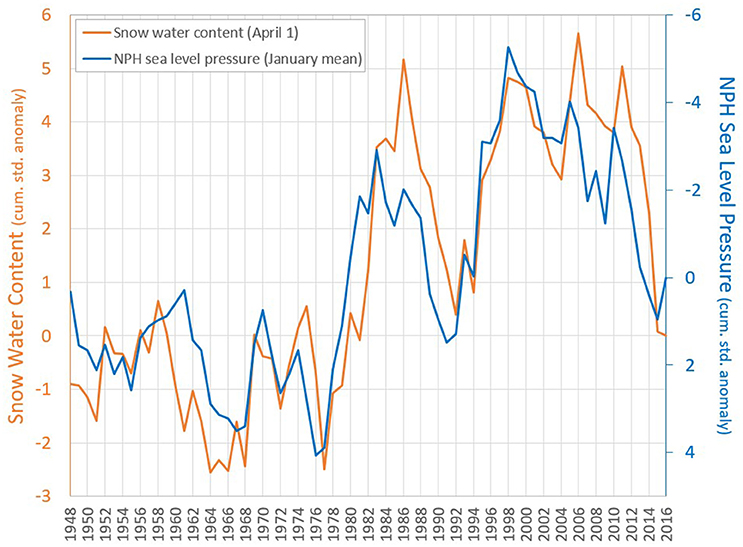
Figure 1. Cumulative standardized anomaly of April 1 snow water content at Mammoth Pass (orange) and January mean sea level pressure at the North Pacific High region [NCEP/NCAR grid cell centered at (35°N, 232.5°E)] (blue). The blue line refers to the vertical axis on the right, where values are in reverse order to aid comparison between the two variables, given that they are inversely correlated.

The Owens Valley snow water content (SWC) on April 1 depends mainly on seasonal precipitation totals but also on factors that influence snowmelt, including temperature, solar radiation and wind. Elevation is sufficiently high that nearly all winter precipitation at the sites of interest is in the form of snow. Years in which snowmelt occurs early will have diminished SWC on April 1. The model presented here does not account for these factors, but relies on the cointegrated relationship between SWC and NPH anomalies.

The cointegrated relationship between SWC and NPH anomalies is explored in the VECM model described in section The VECM Model, for Forecasting the April 1 SWC. The categorical model is described in section the Categorical Model, for Estimating Probability of Dry, Normal, or Wet Categories.

The VECM Model, for Forecasting the April 1 SWC

VECM Model Formulation

Vector Autoregression (VAR) is a type of model that represents multivariate time series using linear relationships between each variable and p of its own lags and the lags of the other variables. If the k x 1 vector y_t denotes the values of the k variables in the multivariate time series at time t, then a VAR(p) model is:

$\begin{array}{ll}{y}_t=a+A_1{y}_{t-1}+A_2{y}_{t-2}+\cdots +A_p{y}_{t-p}+{\epsilon }_t& (1)\end{array}$

Here the vector a (intercept term) and the k x k matrices A_i (coefficients) are estimated model parameters and the vectors ε_t are random errors.

The year-specific vector at time t is given by the difference between the cumulative vectors at times t and t − 1:

$\begin{array}{ll}\Delta y_t=y_t-y_{t-1}& (2)\end{array}$

Combining Equation (1) and (2) and writing B_i = −(A_i+1+⋯+A_p) for each i = 1, ⋯ , p − 1 and Π = −(I − A₁ − ⋯−A_p) gives:

$\begin{array}{ll}\Delta y_t=a+B_1\Delta y_{t-1}+\cdots +B_{p-1}\Delta y_{t-p+1}+\Pi y_{t-1}+{\epsilon }_t& (3)\end{array}$

Cointegration is a property that multivariate time series may exhibit. If the individual components of y_t are non-stationary (in particular, they have a unit root) while some (non-zero) linear combination ${{\beta }^{\prime }y}_t$ is stationary, then y_t is said to be cointegrated. More intuitively, although the components of y_t are non-stationary and vary randomly, the distance between them tends to stay within a fixed distance. In fact, there may be up to h < k linearly independent cointegrated relations among the y_t.

In Equation (3), if y_t is cointegrated then Π has reduced rank h < k and can be factored as Π = αβ′, where α is k × h and β′ is h × k, such that ${\beta }^{\prime }{y}_t$ is a stationary h × 1 vector. Then inference proceeds by first estimating the cointegrated relations β′–either by ordinary least squares (OLS) or maximum likelihood (ML) methods—and then estimating the remaining parameters a, α and β_i by OLS. This type of VAR with reduced rank restrictions when y_t is cointegrated is known as a Vector Error Correction Model (VECM). See Hamilton (1994) and Johansen (1995) for further details.

Data Sets

The observed snow water content (SWC) on February 1 and April 1 of each year, starting 1948, at the four Owens Valley snow stations of interest—Mammoth Pass, Rock Creek #2, Sawmill, and Cottonwood #1—were provided by LADWP and are used as predictor variables in the VECM model.

Also used as a predictor variable in the VECM model is the January mean sea level pressure at a location near the climatological position (i.e., the average position over time) of the NPH. The monthly mean sea level pressure data from the National Center for Environmental Prediction, National Center for Atmospheric Research (NCEP-NCAR) reanalysis dataset (originally described in Kalnay et al., 1996) were used. The data were downloaded from the National Oceanic and Atmospheric Administration's web site¹. This data set was selected for this study because it goes back in time to 1948, covering the entire period of LADWP snow records; has a resolution of 2.5° of latitude and longitude, which is sufficiently fine-scale but not so fine as to have excessive variability over time; and is updated online by NOAA daily, with only a 2-day delay. The grid cell centered at {35°N, 232.5°E} is used.

Reanalysis datasets, such as the ones used in this work, are based on simulations by dynamic climate models combined with observations. Such datasets represent estimates subject to uncertainty, characterized, for example, in Bosilovich et al. (2008), Guirguis and Avissar (2008), and Janowiak et al. (1998).

Because the VECM model uses cumulative standardized anomalies, the raw variables are first transformed into standardized anomalies, by subtracting the series mean then dividing by the standard deviation. The mean and standard deviation values used are for the entire record period, 1948–2016. The standardized anomalies are then added successively over time to obtain the cumulative standardized anomalies.

Parameter Fitting

For fitting, the following steps were followed:

1) Clip the time series to the calibration period.

2) Specify number of lags. This study used p = 3, i.e., the VECM uses two lag terms (years) and the underlying VAR model is VAR(3).

3) Estimate β′ by Full Information Maximum Likelihood (FIML; Johansen, 1995).

4) Estimate parameters a, α and β_i by OLS. Calculate parameters A_i from those.

For prediction, the following steps were followed:

5) Convert back to VAR representation ((β_i, Π) ↦ A_i).

6) Use Equation (1) to calculate the forecasted cumulative value ŷ_t using data from the preceding 3 time periods and with ε_t = 0.

7) Use Equation (2) to obtain the desired forecasted value Δŷ_t = ŷ_t − y_t−1.

Model verification will be described in section VECM Model.

The Categorical Model, for Estimating Probability of Dry, Normal, or Wet Categories

Categorical Model Formulation

The Categorical Model was developed as a complement to the VECM model. The two models are distinct in intent and formulation. The purpose of the Categorical Model is to estimate in early February the probability of the upcoming April 1 SWC falling into each of the three categories, dry, normal, or wet. These probabilities can be denoted p_d, p_n, and p_w, respectively.

The only input to the Categorical Model is the April 1 SWC value forecast by the VECM model. As with any forecast, there is uncertainty in the value forecast by the VECM model, and this implies that in a general sense no one of the three categories—dry, normal, or wet—can be ruled out as a possible outcome. Instead, each category has some non-zero probability of occurring.

Figure 2 shows the forecast for year 2010, as an example. The forecast is indicated by the red line. The red dashed lines indicate the 95% confidence interval, assuming the errors are normally distributed about the forecast value. There is a 5% chance (or 1 in 20 chance) that the observed April 1 SWC will be outside the 95% confidence interval. The blue line is the Gaussian probability density function (PDF), with mean equal to the forecast value and standard error estimated from the 1951–2016 forecasts. The green line is the normal value (the average for 1966–2015), and the dashed green lines indicate a 20% deviation from the normal value. The probability of each category is determined by the area under the Gaussian blue line, lying within the range of values of that category.

FIGURE 2

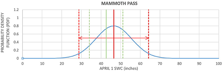
Figure 2. Mammoth Pass April 1 SWC forecasts for year 2010 (red line). The red dashed lines indicate the 95% confidence interval, assuming the errors are normally distributed about the forecast value. The blue line is the Gaussian probability density function (PDF), with mean equal to the forecast value and standard error estimated from the 1951–2016 forecasts. The green line is the normal value (the average for 1966–2015), and the dashed green lines indicate the category boundaries defined by a 20% deviation from the normal value.

Once the VECM model was fit for each location, the Categorical Model estimates the probability that the April 1 SWC value would fall into one of a pre-specified set of water year classes, using the categorical distribution (see for example Murphy, 2012). If there are K categories, the categorical distribution is parametrized by a K-vector θ = (θ₁, …, θ_K) with entries summing to 1. θ_k gives the probability that an observation y falls into category k.

The Categorical model uses the VECM-forecast April 1 SWC value, x, as a predictor for θ via the regression

$\begin{array}{ll}{\theta }_k=a_k+b_k·x,\text{f}\text{o}\text{r}k=1,\dots ,K& (4)\end{array}$

The entries of θ are rescaled to sum to 1 via the softmax function:

$\begin{array}{ll}{\theta }_k=\frac{exp{\theta }_k}{{\displaystyle {\sum }_i}exp{\theta }_i}& (5)\end{array}$

Parameter Fitting

Using Bayesian inference, the model parameters (a_k, b_k) are fit with Markov Chain Monte Carlo (MCMC) to draw samples from the model posterior distribution. All years were used in the model fitting. The following prior distributions were used:

$\{\begin{array}{cc}\begin{array}{c}{a}_k~N\left(0,5\right)\\ b_k~N\left(0,1\right)\end{array}& (6)\end{array}$

Results and Model Evaluation Based on Hindcasts

VECM Model

Model Verification

Parameter fitting was described in methods section Parameter fitting. For model verification, 10 years (2007–2016) were excluded from parameter fitting, to be used for model verification. This 10-year period includes a few wet and some very dry years, thus offering a range of different conditions for verification. In Figures S-10, S-12, S-14, and S-16, the cumulative time series of predictand and predictor variables are plotted (top panel) and the p-value on the top left corner tests the rejection of the null hypothesis that no cointegration is present in the vector time series via the Phillips-Ouliaris-Hansen test (Phillips and Ouliaris, 1990; Hamilton, 1994). The p-values are low for all the stations, indicating that the presence of cointegration cannot be rejected. Figures S-11, S-13, S-15, and S-17 show the observed (black) and VECM-model predicted April 1 SWC (green for the calibration period, 1951–2006, and blue for the verification period, 2007–2016), with the cumulative values on the top panels, and the regular values on the bottom panels. Examination of these figures indicates that the forecasts of the last 10 years have similar deviations from the observations as do those of the years used in parameter fitting.

Final Model Parameters

For the final model parameters, we repeated the parameter fitting, this time including all available years, 1948–2016. The results for Mammoth Pass are displayed in Figure 3. Results for all snow stations are shown in Figures S-18 to S-25.

FIGURE 3

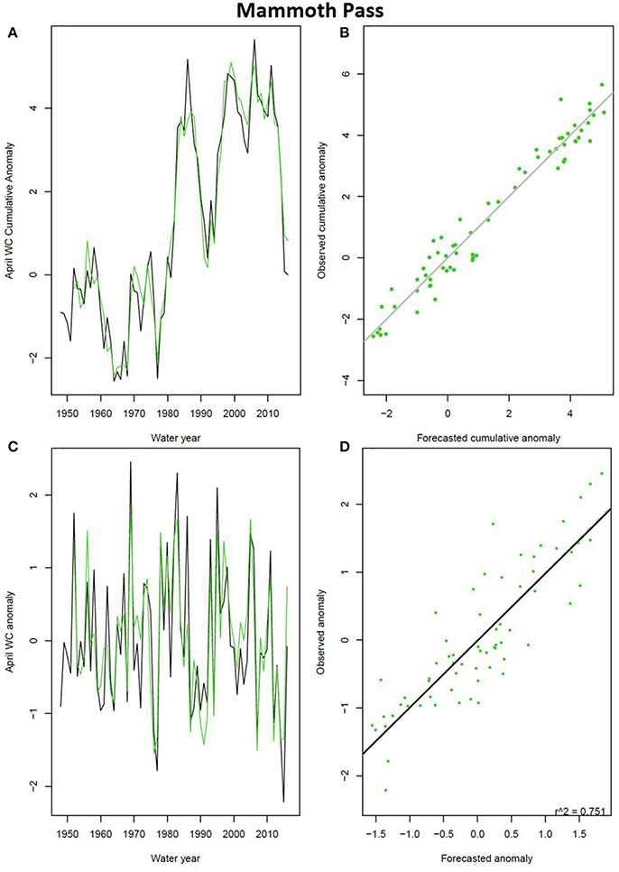
Figure 3. VECM model predictions for Mammoth Pass, using the final parameters. (A) Cumulative April 1 SWC anomalies; (B) Scatter plot of the data in panel A; (C,D) As in panels (A,B) but for the anomalies (not cumulative). Time series lines in black are observed data. Green lines and points indicate VECM model forecasts (1951–2016).

VECM Model Performance Evaluation Using Hindcasts for 1951–2016

The VECM model is evaluated in this section using hindcasts for the period from 1951 through 2016. Because each forecast relies on data from the preceding three years (we have p = 3 in Equation (1) and the record starts in 1948, the first possible forecast is for 1951.

Observations are plotted against forecasts in Figure 4. Values of the coefficient of determination, R², are reported on each figure panel and in Table 1. Dashed lines have been added to each panel of Figure 4 to indicate the 95% confidence interval. Confidence intervals were calculated based on the assumption that the forecasts' deviations from the observations are normally distributed, and characterized by the standard error calculated by comparing forecasted and observed values for all years (1951–2016) (Table S-1).

FIGURE 4

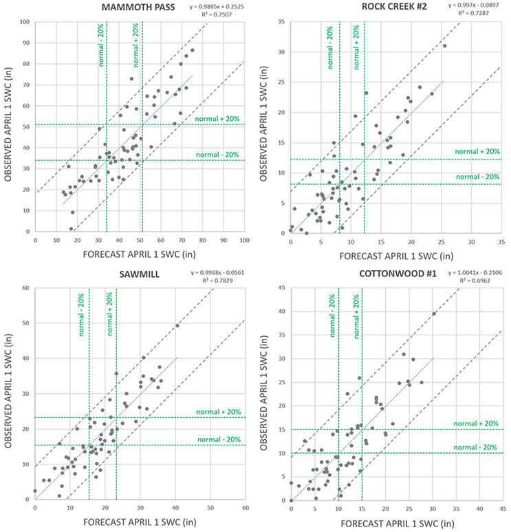
Figure 4. Observed April 1 SWC each year in 1951–2016 plotted against the model's forecast value, for the four Owens Valley sites. Dashed gray lines indicate the 95% confidence interval. Dashed green lines indicate a 20% deviation from the normal value, separating between the categories dry, normal, and wet.

TABLE 1

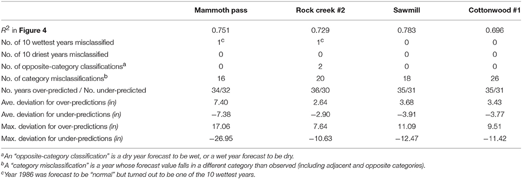
Table 1. Measures of VECM model April 1 SWC forecast performance.

By definition of 95% confidence interval, 5% of the points (i.e., 1 in 20 points) are expected to fall outside the interval in a large sample of points. Here, the sample size of 66 years (1951–2016) is relatively small, so we expect the number of points outside the 95% confidence interval to be in the vicinity of 3.3. The number of points lying outside the 95% confidence interval bounds in Figure 4 is indeed in the vicinity of 3.3: 2 points for Mammoth Pass, 4 points for Rock Creek #2, 3 points for Sawmill, and 6 points for Cottonwood #1.

LADWP defines the normal SWC value at each site as the average of 50 recent years. The 50-year range is updated every 5 years. At the time of writing this manuscript, the 50-year period used by LADWP is 1966–2015, and the normal values are the following:

$Normalvalues:\{\begin{array}{ll}\text{Mammoth}\text{Pass}:\hfill & \text{42}.\text{64}\text{in}\hfill \\ \text{Rock}\text{Creek}\#\text{2}:\hfill & \text{10}.\text{19}\text{in}\hfill \\ \text{Sawmill}:\hfill & \text{19}.\text{33}\text{in}\hfill \\ \text{Cottonwood}\#\text{1}:\hfill & \text{12}.\text{54}\text{in}\hfill \end{array}$

Of special importance to LADWP is an April 1 SWC forecast in the form of three categories:

$\begin{array}{cc}\begin{array}{l}April1\\ SWCCategories:\end{array}& \{\begin{array}{l}\text{Dry}:\text{ Less than 80}\%\text{ of the normal value}\\ \text{Normal}:\text{Within 20}\%\text{ of the normal value}\\ \text{Wet}:\text{ More than 120}\%\text{ of the normal value}\end{array}\end{array}$

The observed frequency of these categories in the 66 years of record are: For Mammoth Pass, 24 dry, 22 normal, and 20 wet years; for Rock Creek #2, 32 dry, 13 normal, and 21 wet years; for Sawmill, 30 dry, 17 normal, and 19 wet years; and for Cottonwood #1, 33 dry, 13 normal, and 20 wet years.

Figure 4 and Table S-2 compares the forecast and observed value of April 1 SWC for each year, and also allows comparison of the forecast category and the observed category (dry, average, or wet). The number of years, from the total of 66 years, which were forecast in the wrong category, is given in Table 1. For Mammoth Pass, which is the most important station for LADWP, given its much larger snowpack, 50 of the 66 years (or 76%) had VECM model forecasts in the same category as observed. The remaining 16 years were misclassified in an adjacent category. For Mammoth Pass, Sawmill, and Cottonwood #1, there were no instances where the forecast value was in the category opposite the observed one, i.e., no dry year was forecast to be wet, and no wet year was forecast to be dry. For Rock Creek #2, there were two instances of opposite-category classifications. In both cases, the forecast was in the dry category, but the observation was in the wet category.

There is considerable agreement between observed categories across the four stations, and though there are several instances where a normal year at one station was dry or wet at another station, there are no instances where one station was dry and another wet in the same year, i.e., opposite categories were not observed across stations. The same is true of the VECM model predictions: in no year was one station predicted to be wet while another station was predicted to be dry. This can be seen in Figure S-26.

Additional measures of the VECM model performance are listed in Table 1. There is no evidence for model bias toward either over-predicting or under-predicting. For Mammoth Pass, the number of over-predicted years, 34, is close to the number of under-predicted years, 32; the average deviation of forecasts to observations is ~ 0 (0.24 in), showing that positive and negative deviations approximately cancel each other out; and the slope of the regression line is ~1.0. For the 34 over-predicted years, the average difference between forecast and observed values is 7.40 in, while for the 32 under-predicted years it is −7.38 in. The largest deviation is 17.06 in for the over-predicted years, and −26.95 in for the under-predicted years.

The year with the largest under-prediction for Mammoth Pass was 1986, where the forecast was for 45.9 in (108% of normal) and the observation was 72.9 in (171% of normal). The year with the largest over-prediction was 2015, where the forecast was for 17.1 in (40% of normal) and the observation was 1.4 in (3% of normal). This was a year when snowmelt occurred earlier than usual, depleting the snowpack before April 1.

Comparison Against Hindcasts Based on February 1 SWC Linear Regression

This section compares the VECM model performance in forecasting April 1 SWC against the results achieved using the historical linear regression equation relating observed April 1 SWC to February 1 SWC based on 1948–2016 observations for each station. The February linear regression method was available prior to this study, and represents a baseline against which the VECM model forecasting skill can be compared.

Skill forecasting the April 1 SWC value

The VECM model was more successful than the February linear regression, when comparing between Table 2 and Table 1 (and between Figures S-29 and S-27). For Mammoth Pass, the coefficient of determination (R²) is 0.751 for the VECM model and 0.630 for the February linear regression. The forecast errors of the February linear regression, i.e., the differences between the forecast value and the observation on the same year, have higher average values and larger maximum values (positive and negative), compared to the VECM model. See also Figures S-28 and S-30.

TABLE 2

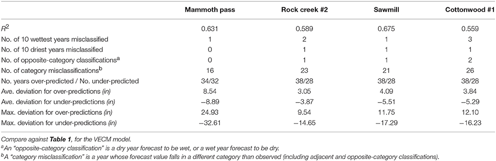
Table 2. Performance measures for forecasts based on the February linear regression equations.

Skill forecasting the April 1 SWC category (dry, normal, or wet)

The VECM model had no instances (for any station) where one of the 10 driest years was misclassified, while the February linear regression had one such instance for each station except Mammoth Pass (Table 2). The VECM model had one instance (for Mammoth Pass and Rock Creek #2) where a top 10 wettest year was misclassified (Table 1), while the February linear regression had one such instance for Mammoth Pass and Sawmill, two instances for Rock Creek #2 and three instances for Cottonwood #1 (Table 2). The VECM model had no instances of a top 10 dry year being misclassified (Table 1), while the February linear regression had one such instance for Rock Creek #2, Sawmill and Cottonwood #1 (Table 2).

Evaluation of the Categorical Model Results Using Hindcasts for 1951–2016

Given the probabilistic nature of the Categorical Model, it is expected that the observed April 1 SWC will often fall into a category (dry, normal, or wet) other than the one to which the model attributed the highest probability of the three. The observed April 1 SWC is expected to most often fall into the category assigned the highest probability, but to also often fall into the category assigned the second-highest probability, and occasionally to fall into the category assigned the lowest probability.

A rigorous evaluation of the Categorical Model's performance would require a much larger sample than the available 66 years (1951–2016). The available 66 years however does allow an approximate evaluation through the qualitative examination of Figure 5, where the probability assigned to category “wet” (p_w) is plotted against the probability assigned to “dry” (p_d). Each point represents a year between 1951 and 2016. Given p_w + p_d + p_n = 1, rearranging that equation we can write p_n = 1–(p_w + p_d), which gives the probability assigned to category “normal” (p_n) is a function of the probabilities plotted in Figure 5. The graph area labeled “most likely wet” corresponds to p_w being larger than either p_d or p_n; “most likely dry” corresponds to p_d > p_w, p_n; and “most likely normal” corresponds to p_n > p_w, p_d.

FIGURE 5

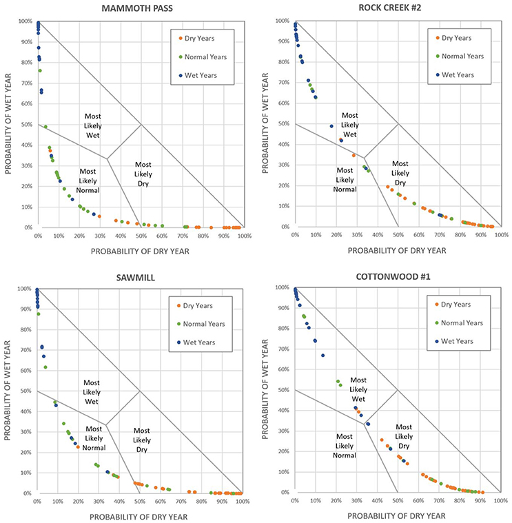
Figure 5. Probability assigned to categories “dry” (x axis) and “wet” (y axis) each year in 1951–2016. The actual observed category each year is indicated in color, according to the legend. The distribution of colors appears consistent with the probabilities.

In Figure 5, the actual observed category each year is indicated by the color of the point, keyed in the figure legend. The distribution of colors appears consistent with the probabilities, with most wet years having been attributed a high probability of being wet, and most dry years having been attributed a high probability of being dry. Because the model provides probabilities rather than predicted values, none of the outcomes represent model failures.

The Categorical Model is designed specifically for assigning probabilities to each of the three categories, not to provide a forecast. If it were used to forecast the category directly, this model would do somewhat less well than the VECM model, especially because of a larger number of opposite-category forecasts (i.e., wet years forecast to be dry, and dry years forecast to be wet) in the period 1951–2016. Therefore, the VECM model forecast April 1 SWC value should be used to forecast the category, and the Categorical Model should be used to evaluate the uncertainty pertaining to the category.

Example: The Probabilities Calculated for 2010

As an example, Figure 6 displays the probabilities determined by the Categorical Model for 2010. The observed SWC values on April 1, 2010, fell into the normal category for all four stations. Even though in the case of Rock Creek #2 and Cottonwood #1 the normal category did not have the highest of the three probabilities (the wet category was assigned higher probability), it nevertheless had considerable probability values: 25.2% for Rock Creek #2, and 9.6% for Cottonwood #1.

FIGURE 6

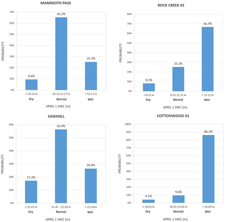
Figure 6. Probability of April 1 SWC falling into each of the categories – dry, normal, or wet – issued by the Categorical Model for 2010.

Forecasts for 2017 and 2018

The VECM model and the Categorical model were parameterized using observations for 1948-2016 (section Methods). The models were completed and delivered to LADWP in January of 2017. Since then, the model has been used to forecast April 1 snow water content (SWC) in 2017 and 2018. These were actual forecasts as opposed to hindcasts. The forecast April 1 SWC is compared against the observed value in Figure 7. The red dots represent 2017 and the orange dots represent 2018. Gray dots are hindcasts for 1951–2016 and were previously shown in Figure 4.

FIGURE 7

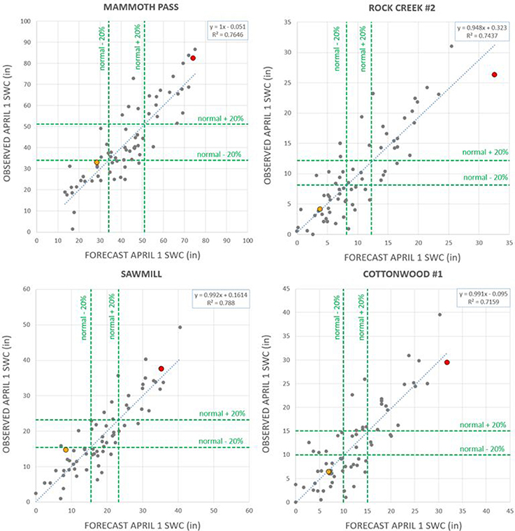
Figure 7. Forecast for years 2017 (red) and 2018 (orange) plotted against the respective observations, for the four Owens Valley sites. The gray points represent 1951–2016 hindcasts, previously shown in Figure 4.

Year 2017 had among the largest snowpack of the period plotted, especially at the most important station, Mammoth Pass. On February 1, the observed SWC was already almost double the normal (i.e., average) value for that date at Mammoth Pass and Sawmill, and more than triple the normal value at Rock Creek #2 and Cottonwood #1. By April 1, the observed SWC was about double the normal value for that date at Mammoth Pass and Sawmill, and about 2.5 times the normal at Rock Creek #2 and Cottonwood #1. The VECM model provided April 1 SWC forecasts that were mildly over-estimated for Mammoth Pass and Sawmill, and slightly under-estimated for Rock Creek #2 and Cottonwood #1 (Figure 7). The Categorical model correctly identified “wet” (i.e., more than 20% above the normal value) as the most likely category for April 1 SWC at all four stations.

Year 2018 was a more complex year, representing a good test case. SWC was very low on February 1 but, thanks to late-season storms in February and March, it reached near-normal values on April 1. The VECM model correctly forecast these near-normal values. For example, on February 1, the SWC at Rock Creek #2 was at 10% of the normal value for that date; but on April 1 had reached 40% of the normal value for that date. The VECM model correctly forecast the substantial SWC increase that occurred in February and March, producing approximate forecasts for the four stations (Figure 7). The Categorical model correctly identified “dry” (i.e., more than 20% below the normal value) as the most likely category for April 1 SWC at all four stations, with “normal” also having reasonable probability. For example, at Mammoth Pass, the probability of “dry” was 77.9% and the probability of “normal” was 21.9%. The observed April 1 SWC was “dry” but near “normal.”

Conclusions

The VECM model developed and tested in this study has proven to have considerable skill forecasting Owens Valley April 1 SWC in early February. Its performance in hindcasts (1951-2016) was shown to surpass the skill of the pre-existing alternative, which consisted of using a linear regression to forecast April 1 SWC based on the observed February 1 SWC. The VECM model's performance was clearly superior to the February linear regression on every measure, including a higher coefficient of determination (R²), smaller average and maximum errors (defined as the forecast value minus observed value), fewer misclassifications of years, defined as a year when the forecast and observed April 1 SWC are not in the same category (dry, normal, or wet), and fewer severe misclassifications of years (i.e., years forecast to be in the category opposite the observed one, especially when those were extreme years such as among the 10 wettest or 10 driest).

As a complement to the VECM model, the Categorical Model was developed to express forecast uncertainty by estimating the probability that April 1 SWC would fall into each of the three categories—dry, normal, and wet. While the sample size of the hindcast (66 years: 1951-2016) is too small for rigorous testing of the Categorical Model, the probabilities it produced for these hindcast years appear consistent with the observations. The VECM model forecast April 1 SWC value should be used to also forecast the category, and the Categorical Model should be used to evaluate the uncertainty pertaining to the category.

Since the model was completed, using 1948-2016 observations, it model has been used to forecast April 1 snow water content (SWC) in 2017 and 2018. These were actual forecasts as opposed to hindcasts. The 2017 and 2018 forecasts were compared against the observed April 1 SWC values, showing to have been successful and having deviated no more from observations than most years in the hindcast period. The Categorical model also attributed the highest probability to the category that was observed on April 1. The 2017 was an exceptionally wet year, and 2018 was overall a dry year but which received late-season storms in February and March. The successful forecast in both 2017 and 2018 adds confidence in the VECM model and the Categorical model.

While the VECM model was shown to provide considerable forecast skill for April 1 SWC, there is significant uncertainty associated with its forecast in any individual year. This is the case with any meteorological or hydrological forecast model. Model uncertainty was clearly characterized in this report using hindcasts. Future forecasts may incur smaller or larger errors than those seen in the hindcasts or the two forecast years of 2017 and 2018. Forecast uncertainty must therefore be taken into account by LADWP in its decision making.

Wider Significance of This Work, and Future Research

Many water supply reservoirs in California capture snowmelt in spring for supply later in summer. Under current operations, some reservoir storage is set aside for future floods over the course of the wet season—the flood control volume varying by month—and excess runoff is released downstream (e.g., Willis et al., 2011). The statistical tool presented in this work, relating NPH anomaly to precipitation or snowpack indices, can be applied to other California watersheds, where it may allow reservoir operators additional insight, on a year-to-year basis, on whether some of the flood storage could be utilized for water supply storage. This additional insight could be of great value in coming decades, where operators must make the most from a potentially more variable precipitation season, as well as declining snowpack due to higher temperatures and a partial shift from snowfall to rainfall, and greater peaks in runoff in wet years (Fissekis, 2008; Brekke et al., 2009; Hanak and Lund, 2012).

The forecasting tool presented in this paper allows issuing forecasts in early February for the remainder of the wet season, i.e., through April 1. The tool is based on the sea-level pressure anomaly at the climatological location of the NPH measured in mid-January.

The forecast lead time may potentially be increased if the mid-January NPH sea level pressure anomaly can be accurately forecasted, whether by statistical or dynamical models. The NPH exhibits a closer relationship with precipitation throughout California compared to the ENSO indices (see Costa-Cabral et al., 2016). This may be because, in addition to tropical forcing, the NPH also receives influence from internal midlatitude variability. However, the question remains whether this internal midlatitude variability may or may not be forecastable.

This work demonstrates that advancements in forecasts of NPH are expected to have significant benefits for water resources, agriculture, energy, insurance, drought preparedness, and flood risk management in California. We hope that future research will investigate the present ability of the different models in the North American Multi-Model Ensemble (NMME; Kirtman et al., 2014) suite [which includes NOAA's National Weather Service Climate Forecast System, version 2 (CFSv2; Saha et al., 2014)] to anticipate the NPH anomaly in mid-January at different lead times.

This work may also contain important hints for future research by climate scientists. The cointegrated relationship identified means that the principal relationship between these 2 variables (NPH anomalies and California precipitation) is between their integrals. This suggests that the climate processes involved have characteristics analogous to reservoirs, which are integrals of stochastic inputs and outputs. This line of thinking, if further explored, might bear fruit in understanding the low-frequency variability in climate, such as decadal variability. Precipitation depends on ocean surface temperatures (SST) at different locations. Temperature measures heat content, a reservoir type variable which may be at the origin of cointegrated relationships between climatic variables.

Author Contributions

MC-C led this study and had the idea of using cointegration as the basis for the forecasting model; JR suggested the VECM model and the categorical model mathematical frameworks, fitted the model parameters, and encoded these models in Excel for operational use; MC-C conducted the hindcasts and model evaluation, and respective graphics, and wrote most of the text of this manuscript.

Conflict of Interest Statement

The authors declare that the research was conducted in the absence of any commercial or financial relationships that could be construed as a potential conflict of interest.

Acknowledgments

This work was commissioned and funded by the Los Angeles Department of Water and Power (LADWP). We thank LADWP for the opportunity of developing this forecasting approach and applying it to the Owens Valley watershed. Sujoy B. Roy provided comments that improved the quality of this manuscript, and his contribution is gratefully acknowledged. Two reviews contributed to clarity and a more expanded discussion in this paper, and are gratefully acknowledged. The preparation of this manuscript was funded by the employers of the two authors, Northwest Hydraulic Consultants Inc, and Tetra Tech Inc.

Supplementary Material

The Supplementary Material for this article can be found online at: https://www.frontiersin.org/articles/10.3389/feart.2018.00054/full#supplementary-material

Footnotes

1. ^ http://www.esrl.noaa.gov/psd/data/gridded/data.ncep.reanalysis.derived.surface.html (file name: slp.mon.mean.nc)

References

Brekke, L. D., Maurer, E. P., Anderson, J. D., Dettinger, M. D., Townsley, E. S., Harrison, A., et al. (2009). Assessing reservoir operations risk under climate change. Water Resour. Res. 45:W04411. doi: 10.1029/2008WR006941

CrossRef Full Text | Google Scholar

Bosilovich, M., Chen, J., Robertson, F. R., and Adler, R. F. (2008). Evaluation of global precipitation in reanalyses. J. Appl. Meteor. Climatol. 47, 2279–2299. doi: 10.1175/2008JAMC1921.1

CrossRef Full Text | Google Scholar

Chikamoto, Y., Timmermann, A., Luo, J. J., Mochizuki, T., Kimoto, M., Watanabe, M., et al. (2015). Skilful multi-year predictions of tropical trans-basin climate variability. Nat. Commun. 6:6869. doi: 10.1038/ncomms7869

PubMed Abstract | CrossRef Full Text | Google Scholar

Costa-Cabral, M., Rath, J. S., Mills, W. B., Roy, S. B., Bromirski, P. D., and Milesi, C. (2016). Projecting and forecasting winter precipitation extremes and meteorological drought in California using the North Pacific High sea-level pressure anomaly. J Clim. 29, 5009–5026. doi: 10.1175/JCLI-D-15-0525.1

CrossRef Full Text | Google Scholar

Costa-Cabral, M., Roy, S. B., Maurer, E. P., Mills, W. B., and Chen, L. (2012). Snowpack and runoff response to climate change in owens valley and mono lake watersheds. Clim. Change 116, 97–109. doi: 10.1007/s10584-012-0529-y

CrossRef Full Text | Google Scholar

Engle, R. F., and Granger, C. W. J. (1987). Co-integration and error correction: representation, estimation and testing. Econometrica 55, 251–276.

Google Scholar

Fernando, D. N., Fu, R., Solis, R. S., Mace, R. E., Sun, Y., Yang, B., et al. (2015). Early Warning of Summer Drought Over Texas and the South Central United States: Spring Conditions as a Harbinger of Summer Drought. Technical Note 15-02, Texas Water Development Board.

Fissekis, A. (2008). Climate Change Effects on the Sacramento Basin's Flood Control Projects. M. S. thesis, Department of Civil and Environmental Engineering, University of California, Davis, CA, 150 pp.

Guirguis, J., and Avissar, R. (2008). An analysis of precipitation variability, persistence, and observational data uncertainty in the western United States. J. Hydrometeor. 9, 843–865, doi: 10.1175/2008JHM972.1

CrossRef Full Text | Google Scholar

Hamilton, J. D. (1994). Time Series Analysis. Princeton, NJ: Princeton University Press.

Google Scholar

Hanak, E., and Lund, J. R. (2012). Adapting California's water management to climate change. Clim. Change 111, 17–44. doi: 10.1007/s10584-011-0241-3

CrossRef Full Text | Google Scholar

Janowiak, J., Gruber, A., Kondragunta, C. R., Livezey, R. E., and Huffman, G. J. (1998). A comparison of the NCEP–NCAR reanalysis precipitation and the GPCP rain gauge–satellite combined dataset with observational error considerations. Clim. J. 11, 2960–2979. doi: 10.1175/1520-0442(1998)011 < 2960:ACOTNN>2.0.CO;2

CrossRef Full Text

Johansen, S. (1995). Likelihood-based Inference in Cointegrated Vector Autoregressive Models. Oxford, UK: Oxford University Press.

Kalnay, E., Kanamitsu, M., Kistler, R., Collins, W., Deaven, D., Gandin, L., et al. (1996). The NCEP/NCAR 40-year reanalysis project. Bull. Amer. Meteor. Soc. 77, 437–471. doi: 10.1175/1520-0477(1996)077 < 0437:TNYRP>2.0.CO;2

CrossRef Full Text | Google Scholar

Kharin, V. V., Zwiers, F. W., Zhang, X., Hegerl, G., and Wehne, M. (2013). Changes in temperature and precipitation extremes in the CMIP5 ensemble. Clim. Change 119, 345–357. doi: 10.1007/s10584-013-0705-8

CrossRef Full Text | Google Scholar

Kirtman, B. P., Min, D., and Infanti, J. M. (2014). The North American multimodel ensemble. phase-i seasonal-to-interannual prediction; phase-ii toward developing intraseasonal prediction. Bull. Amer. Meteor. Soc. 95, 585–601. doi: 10.1175/BAMS-D-12-00050.1

CrossRef Full Text

Mantua, N. H., Hare, S. R., Zhang, Y., Wallace, J. M., and Francis, R. C. (1997). A Pacific interdecadal climate oscillation with impacts on salmon production. Bull. Amer. Meteor. Soc. 78, 1069–1079. doi: 10.1175/1520-0477(1997)078 < 1069:APICOW>2.0.CO;2

CrossRef Full Text | Google Scholar

Murphy, J. P. (2012). Machine Learning: a Probabilistic Perspective. Cambridge, MA: MIT press.

Pandey, G. R., Cayan, D. R., and Georgakakos, K. P. (1999). Precipitation structure in the Sierra Nevada of California during winter. J. Geophys. Res. 104, 12019–12030. doi: 10.1029/1999JD900103

CrossRef Full Text

Phillips, P. C. B., and Ouliaris, S. (1990). Asymptotic properties of residual based tests for cointegration. Econometrica J. Econometric Soc. 58, 165–193. doi: 10.2307/2938339

CrossRef Full Text | Google Scholar

Saha, S., Moorthi, S., Wu, X., Wang, J., Nadiga, S., Tripp, P., et al. (2014). The NCEP climate forecast system version 2. Clim. J. 27, 2185–2208. doi: 10.1175/JCLI-D-12-00823.1

CrossRef Full Text

Stevenson, S., Timmermann, A., Chikamoto, Y., Langford, S., and DiNezio, P. (2015). Stochastically generated North American megadroughts. J Climate, 28, 1865–1880. doi: 10.1175/JCLI-D-13-00689.1

CrossRef Full Text | Google Scholar

Swain, D. L., Tsiang, M., Haugen, M., Singh, D., Charland, A., Rajaratnam, B., et al. (2014). Explaining extreme events of 2013 from a climate perspective. Bull. Amer. Meteor. Soc. 95, S1–S104. doi: 10.1175/1520-0477-95.9.S1.1

CrossRef Full Text

Wang, S.-Y., Hipps, L., Gillies, R. R., and and, J.-,Yoon, H. (2014). Probable causes of the abnormal ridge accompanying the 2013-2014 California drought: ENSO precursor and anthropogenic warming footprint. Geophys. Res. Lett. 41, 3220–3226. doi: 10.1002/2014GL059748

CrossRef Full Text | Google Scholar

Wang, S.-Y., Huang, W.-R., and Yoon, J.-H. (2015). The North American winter ‘dipole' and extremes activity: a CMIP5 assessment. Atmos. Sci. Lett. 16, 338–345. doi: 10.1002/asl2.565

CrossRef Full Text | Google Scholar

Willis, A. D., Lund, J. R., Townsley, E. S., and Faber, B. A. (2011). Climate change and food operations in the Sacramento Basin, California. San Francisco Estuary Watershed Sci. 9, 1–18, doi: 10.15447/sfews.2011v9iss2art3

CrossRef Full Text | Google Scholar

Zhang, U., Wallace, J. M., and Battisti, D. S. (1997). ENSO-like interdecadal variability: 1900–93. Clim. J. 10, 1004–1020. doi: 10.1175/1520-0442(1997)010<1004:ELIV>2.0.CO;2

CrossRef Full Text | Google Scholar